Applications of symmetry in point-line-plane frameworks ...

Applications of symmetry in point-line-planeframeworks for CAD

Patrick W. FowlerDepartment of Chemistry, University of Sheffield,

Sheffield S3 7HF, UK

Simon D. GuestDepartment of Engineering, University of Cambridge,

Trumpington Street, Cambridge CB2 1PZ, UK

John C. OwenSiemens, Francis House,

112 Hills Road, Cambridge CB2 1PH, UK

December 9, 2020

Abstract

Computer-aided design (CAD) typically deals with geometries (points,lines and planes) subject to constraints on distances and angles. Sim-ple counting of freedoms and constraints, as used in the analysis ofengineering structures, also provides a useful condition on the resid-ual freedoms of a CAD drawing. Here we derive general symmetry-extended counting equations to account more fully for the balanceof freedoms and constraints in 2D point-line and 3D point-line-planeframeworks. General forms are given for symmetries of the freedomsof points, lines and planes, and constraints based on distances andangles. The resulting toolkit can be used to give stronger conditionson dimensioning of CAD drawings. This importation to CAD of aphysical point of view, in which residual freedoms correspond to themechanisms and redundant constraints to the states of self-stress ofa structure composed of bodies and joints, can often reveal hiddenfreedoms and redundancies in CAD systems. Point-group symmetryis not a panacea: mechanisms that depend on specific geometries mayescape detection by symmetry alone. One systematic limitation of

1

this type is proved for polyhedra with planar faces and prescribededge lengths.

1 Introduction

Constraint solving is an important aspect of computer-aided design (CAD),and there is a considerable literature that deals with movability of kinematicmechanisms/linkages and geometric constraint solving (Owen, 1991; Boumaet al., 1995; Kim et al., 1998; Barton et al., 2009; Muller, 2016; Sitharam et al.,2019). This paper takes a cross-disciplinary approach to the consideration ofsystems of points, lines and planes subject to constraints that can be specifiedin terms of distances and angles. Such configurations give representations ofphysical systems that may be simple but are sufficient to encompass manyengineering structures and mechanisms and they are already versatile enoughto allow description of the balance of geometric freedoms and constraintsinvolved in setting up and dimensioning engineering drawings. There is aclose analogy between these two types of application. For example, setsof points with distance constraints are precisely analogous to bar-and-jointframeworks in structural engineering. Symmetry analysis of such frameworks,and generalisations to other combinations of bodies and joints have provedfruitful (Fowler and Guest, 2000; Guest and Fowler, 2005; Owen and Power,2010; Guest et al., 2010). Here we adapt and extend this analysis to thegeneral case of a set of points, lines and planes that is subject to constraints.

The basic objects in the present analysis are geometries (points, linesand planes), which are ‘decorated’ as needed with motifs to represent theapplicable constraints mathematically in a way that avoids singularities. Forexample, signed distances are used in 2D to give a non-singular description ofthe point-line distance constraint that continues smoothly to the case whenthe point lies on the line; in the drawings used in the present paper, thisconstraint would be represented by decorating the line with a perpendiculardisplacement arrow. In effect, we are treating lines in 2D and planes in 3Das half-spaces (Jackson and Owen, 2016).

In the spirit of Maxwell counting (Maxwell, 1864; Calladine, 1978) inengineering, for the present application to drawings we first establish thefreedoms associated with geometries and the constraints imposed by the var-ious distance and angle conditions. We count these in order to establish thenumber of residual freedoms in a drawing, which would correspond in theengineering context to the net mobility in a structure. Then we find sym-metry extensions to Maxwellian and Calladinean counting rules for systemsof points and lines in 2D and of points, lines and planes in 3D. The theory

2

of group representations when applied to the symmetry-extended freedomcount can often detect the presence of redundant constraints and excess free-doms in a drawing, even when this is not detected by the simple freedomcount.

Such symmetry techniques have often been used in an engineering contextwhere the requirement is to describe a system that has mobility (Fowler andGuest, 2005). Each application requires some tailoring to the types of objectunder consideration, whether bars, bodies and joints as in engineering, orgeometries and constraints, as here. For applications in CAD, the perspec-tive is further extended, in that we are also interested in finding solutions tothe constraint equations (i.e. determining the coordinates of the geometries)for given values for the constraints (such as the distances between pairs ofpoints and lines or the angle between pairs of lines) (Owen, 1991). Typically,we may be given approximate coordinates for the geometries and requiredto find precise coordinates nearby that satisfy the constraints exactly. Aconsequence of the inverse function theorem (Spivak, 1965) is that for ev-ery excess freedom detected by symmetry there is a corresponding locallyredundant constraint, which means it can be removed without affecting thesolution space in the neighbourhood of the configuration.

An important property of the constraint equations is that they may bequadratically solvable, by which we mean they can be solved using only thesuccessive solution of quadratic equations, equivalent to the classical notionof constructibility with ruler and compasses (Jackson and Owen, 2019). Thefact that some constraints are locally redundant can make it easy to deter-mine that the constraint equations are quadratically solvable and hence tosolve them, as we show in examples below.

The plan of the paper is as follows. In §2 the groundwork is laid for theguiding analogy between concepts in CAD and structural engineering, andan example shows the useful role of symmetry in recognition of potentialproblems with dimensioning of drawings. Counting rules, both scalar andsymmetry-extended, are worked out for systems of points, lines and planes(§3). In §4, general expressions for the symmetries of the respective freedomsare obtained (Eqns (4.1) to (4.4), and (4.9)). In §5, symmetries for the varioustypes of distance and angle constraints are tabulated (Figures 3 and 4). Asdescribed in §6, this tabulation gives a toolkit for use with the overall mobilityequation (6.1) in applications to specific systems. Examples where symmetry-extended equations detect hidden freedoms and redundant constraints inCAD systems are given in §7. There are some systematic limitations onthe information that a pure symmetry approach can provide. A generalresult in §8 shows cancellation of symmetries of freedoms and constraintson geometries in polyhedra with planar faces and fixed edge lengths. A

3

detailed treatment is given in §9 of freedoms and constraints for the frequentlyencountered case of the cubic polyhedral cage (3D embedding of a cubicpolyhedral graph), of relevance to CAD, structural mechanics, and design ofchemical force fields. The paper ends with some brief conclusions.

2 CAD, structural engineering and symme-

try

The upper panel of Figure 1 shows two similarly dimensioned drawings, whichwere created in the commercial design system NX from Siemens. A drawingis said to be fully dimensioned if it has enough dimensions and annotationsto enable precise replication on a drawing board or in another CAD system.If any small, but non-zero, change to each dimension value in turn (keepingthe others unchanged) determines another dimensioned drawing, then thedrawing is said to be independently dimensioned. A drawing which is bothfully and independently dimensioned is said to be well dimensioned.

Comparison of the upper and lower drawings in Figure 1(a) shows thatthey are not fully dimensioned, since the height of the horizontal constructionline is different in the two drawings. The reader can easily verify that, forany reasonable positioning of the horizontal construction line, the drawingcan be made by ignoring any one of the dimensioned line segments in theleft-hand part of the drawing and any one in the right-hand part of thedrawing. The drawing can then be constructed sequentially (using only rulerand compasses). On completion, the removed segments will be found tohave the required length. This shows that the drawing is neither fully norindependently dimensioned.

The lower panel, Figure 1(b), shows two slightly modified drawings inwhich the reflection symmetries of the drawing have been broken in distinctways. In the upper drawing, the overall reflection symmetry is maintainedand the internal reflection symmetry within the component pieces is broken.In the lower drawing, the symmetry of the component pieces is maintainedbut the overall symmetry is broken. The reader is invited to determine whichof these, if either, is well dimensioned.

In fact, the upper drawing is well dimensioned whereas the lower drawingis not. The methods to be described in this paper can be used to provethat the lower drawing is neither independently nor fully dimensioned. Allvariants of the lower drawing can be constructed sequentially with ruler andcompasses using the method described above.

The upper drawing is almost certainly not constructible with ruler and

4

(a)

(b)

Figure 1: Four CAD drawings of the same basic design with different dimen-sion values. Of these, only the upper drawing of (b) is well dimensioned.

5

compasses (Owen, 1991) and requires a CAD system that has a numericalconstraint solving capability. This drawing was made using the 2D DCMconstraint solver, which was developed by one of the authors and colleaguesand is incorporated into the NX product from Siemens and into many othercommercial CAD products. The fact that the upper drawing is well dimen-sioned is easily verified in 2D DCM by showing that the Jacobian matrixof the system of constraint equations has independent rows and maximumrank.

The group representation methods used in this paper to determine thebalance of freedoms and constraints were first applied in the analysis of therigidity of structures (Kangwai and Guest, 1999; Guest and Fowler, 2005,2007). As this field uses terminology rather different from that used in CADand constraint solving, we will describe the relationship between them withthe aid of our example.

From a CAD perspective, the drawing consists of eight line segments (eachwith a length specified by the dimensions) and one construction line. Fourof the line segments have an end point whose coordinates can be specifiedindependently as (−20, 0) and (20, 0) and the other four have an end pointwhich has a zero y-coordinate. A completely free line segment has threefreedoms corresponding to rigid body motions. Hence, four of the segmentshave one freedom and the other four have two freedoms giving a total oftwelve freedoms. Two of the segments are automatically connected becausetheir endpoints include a pair with the same coordinates. Connectivity of theends of other segments, which lie on the x-axis, introduces two constraintsand connectivity of the segments at the remaining four points introduceseight further constraints. The construction line ensures that four of thecommon segment ends are collinear, and since any two points are collinearthis introduces two further constraints. There is a total of twelve freedomsand twelve constraints which gives a residual freedom count of zero andsuggests that the drawing might be fully dimensioned.

This process of counting freedoms and constraints is automated in dimen-sional constraint solving software. We describe briefly how this is done inthe 2D DCM software component. A line segment is broken into two pointsand a line. Each point is constrained to be coincident with the line, andthe length of the segment is specified by a distance dimension between thetwo points. Line segments with a common endpoint share the same point.Construction lines are represented as lines and the x- and y-axes are alsorepresented as ‘fixed’ lines. Unfixed points and lines each have two freedoms.Each of the four drawings in Figure 1 has eight points, eleven lines (two ofwhich are fixed), twenty-four point-line coincident constraints, two point-linedistance constraints and eight point-point distance constraints. Again, this

6

gives a residual freedom count of zero.In structural engineering terms, this design corresponds to a bar-joint

framework with two slider joints. Each point corresponds to a joint and eachdimension between two points corresponds to a bar. Two of the joints arepinned. The construction line and the x-axis each correspond to a sliderjoint. Each unpinned joint has two positional freedoms (in 2D) and each barimposes one constraint. The slider joints each impose two constraints. Thenet mobility of the structure is zero.

The difference between the number of freedoms and constraints is knownas the net mobility of a structure and corresponds to the residual freedoms ina drawing. A drawing is fully dimensioned if the corresponding structure isrigid, and well dimensioned if the corresponding structure is minimally rigid.

The Jacobian matrix in constraint solving is called the rigidity matrixin structural engineering (with each row of the matrix divided by 2). Thismatrix has a column for each freedom and a row for each constraint. Thenumber of residual freedoms, which corresponds to the net mobility, is thedifference between the number of rows and columns.

Vectors in the kernel of the rigidity matrix are called flexes (or infinitesi-mal mechanisms), and vectors in the cokernel are called self-stresses (namedafter the corresponding internal equilibrium forces that can therefore exist).The kernel of the rigidity matrix has a subspace of internal flexes which areorthogonal to the infinitesimal rigid body motions. The dimension of thespace of self-stresses is denoted by s and that of the space of internal flexesby m. The rigidity matrix determines the first order or infinitesimal rigidityproperties of the structure, which is said to be infinitesimally rigid if m = 0,and infinitesimally independent if s = 0. A basic theorem of linear algebrastates that the difference between the numbers of columns and rows of amatrix is equal to the difference between the dimensions of its kernel andcokernel. This is known in structural engineering as the Maxwell/Calladinerelation (or counting rule). If s = 0, then rigidity and infinitesimal rigid-ity are equivalent. If m = 0, then s gives the number of locally redundantconstraints. A structure is called isostatic if both m = 0 and s = 0.

As the examples in Figure 1 show, a drawing may not be well dimensionedeven though it has a residual freedom count of zero. This happens for specialpositions of the geometry. Similar examples are studied in robotics. Forexample, a Stewart-Gough platform is known to have an ‘internal’ motion ifthe upper joints lie on a conic and the lower joints also lie on a conic and thesetwo conics are in projective equivalence (Nawratil, 2013). In our case, we usemethods from group theory to show that drawings with no residual freedomsmay not be well dimensioned, owing to the interplay between symmetry inthe dimensioning scheme and symmetry in the positions of the geometries.

7

This property also leads to redundant dimensions and often allows the simpleconstruction of drawings that would otherwise be difficult without numericalmethods.

The essential idea we use is that if a structure or drawing (or part of adrawing or structure) is symmetrical then both the geometries and the con-straints can be viewed separately under each symmetry operation (Kangwaiand Guest, 1999). A geometry is unshifted if its coordinates are left un-changed by the symmetry operation. A pairwise constraint is unshifted ifeither both geometries connected by the constraint are unshifted, or bothare of the same type and their coordinates are exchanged. It is clear fromlinear algebra that a structure cannot be infinitesimally rigid if a count of theresidual freedoms is greater than zero and from the inverse function theoremthat it cannot be rigid if in addition it has no states of stress. Similarly, itcan be shown that the structure cannot be infinitesimally rigid if a countof the residual freedoms (suitably defined) of only the unshifted geometryand constraints is greater than zero (Owen and Power, 2010). In this case,group representation theory may also imply the symmetry of the flexes anddetermine whether they preserve the original symmetry of the structure. Ifthe original symmetry is preserved and there are no self-stresses with thesame symmetry (or which are fully symmetric), then the structure supportsa finite motion (a continuous flex) (Schulze, 2010) and the correspondingdimensioned drawing is not fully dimensioned.

The freedom count that is assigned to a geometry under a symmetryoperation is the trace of the transformation matrix which describes the effectof the operation on the geometry coordinates. For example, a point in 2Dhas zero freedom count under a reflection (which reverses one of a pair oforthogonal translations and preserves the other) whereas it has a count of−2 under a half-turn rotation (which reverses translations in both x- andy- directions). Similarly, the effective number of freedoms removed by aconstraint may depend on the type of constraint and the symmetry operation.In the following sections we show how these numbers are computed andprovide a complete tabulation for points, lines and planes in 2D and 3D andfor various constraints between them.

3 Points, lines and planes

Scalar counting Points in 2D each have two degrees of freedom, and pointsin 3D have three. Lines in 2D have two degrees of freedom (a translationperpendicular to the line direction and a rotation in the plane). Lines in 3Dhave four degrees of freedom (translations along, and rotations about, two

8

independent axes perpendicular to the line). For lines, these freedoms can beconsidered as the set of all possible rigid-body motions with subtraction (in2D) of the translation along the line, or (in 3D) of this translation and therotation about the line. Another justification for the 4-parametric nature ofthe family of 3D lines is via Plucker coordinates, which are 6-tuples subject tothe quadratic constraint known as Klein’s quadric (Plucker, 1865b,a; Klein,1870).

A plane has three degrees of freedom, which we may consider as onefreedom to translate along the normal to the plane and two freedoms torotate about independent in-plane axes. We may also regard these freedomsas derived from the six freedoms of rigid-body motion by exclusion of thesingle rotation about the plane normal and the pair of translations orthogonalto the plane normal.

Hence, the Maxwell/Calladine counting rule for the net mobility of asystem of points, lines and planes is (in 3D and 2D):

3D: m− s = 3P + 4L+ 3S − C − 6, (3.1)

2D: m− s = 2P + 2L− C − 3, (3.2)

where P , L and S are the numbers of points, lines and planes, and C isthe total number of freedoms removed by constraints. Constraints may beimposed on distances (D) of types labelled PP , PL, PS, LL, LS, SS in 3D,or PP , PL, LL in 2D, or on angles (A) of types labelled LL, LS, SS in 3D,or LL in 2D. A constraint typically removes a single degree of freedom, butmay in some settings remove more. Finally, the constant terms of −6 and −3on the right-hand sides of (3.1) and (3.2) account for removal of rigid-bodymotions of the whole system.

The mobility equations (3.1) and (3.2) give the balance m−s, but do notdetermine m and s separately. Further information on m and s may often beobtained by extending pure counting equations such as these to account forsymmetries of mechanisms and states of self-stress (Fowler and Guest, 2000;Guest and Fowler, 2005).

Symmetry-extended counting In CAD, a constrained system of points,lines and planes is usually described by a graph in which the vertices arelabelled with the type of geometry (point, line or plane) that they represent,and likewise the edges are labelled with the type of constraint (distance orangle) that they represent.

A constrained system of points, lines and planes has a point group G

consisting of the symmetry operations that leave the system as a whole

9

unchanged. The general principle behind the construction of symmetry-extended versions of counting relations of the Maxwell-Calladine type is thatall components of an object occur in sets that themselves have well spec-ified behaviour under the symmetries of the object itself. This extends todecorations of the object with sets of scalars, vectors or other local sym-bols and motifs. Consideration of these symmetries allows construction of asingle symmetry-extended counting rule that embodies the ordinary scalarMaxwell/Calladine count as a special case, and in favourable cases adds fur-ther conditions on the separate contributions of m and s to the generalisedmobility count.

In the present application, the sets of structural components, freedomsand constraints have characters χ(g) under the various symmetry operationsg ∈ G, which define their (typically reducible) representations Γ. (For defini-tions and use of terms, see our earlier papers and standard texts (Altmannand Herzig, 1994; Bishop, 1973)). Symmetry operations do not mix geome-tries or constraints of different types.

An illustration for a simple case is given in Figure 2. The point group con-sidered is C2v, with a list of four symmetry elements, consisting of the iden-tity E; an axis of two-fold rotation, C2; and two orthogonal mirror planes, σ1and σ2 (Figure 2(a)). The character table (Figure 2(b)) is generated from thegroup multiplication table by standard methods (see, e.g., (Griffith, 2009)),and here has four irreducible representations, A1, A2, B1 and B2. Hence, thepossible symmetry behaviour of any set of structural components or localmotifs of a C2v-symmetric object is described by some linear combination ofthese. The figure shows the contrasting nodal behaviour of scalar functionsof each type (Figure 2(c)), and then illustrates (Figures 2(d)-2(g)) the waysin which they combine to give reducible representations for sets of scalarsand vectors associated with vertices and edges of a simple geometrical objectin a C2v setting. Representations can be added and multiplied, character bycharacter, according to standard rules (Altmann and Herzig, 1994; Bishop,1973).

Our aim here is to establish relations between the symmetries of geome-tries, freedoms and constraints to act as symmetry-extended parallels to thescalar counting rules. A comprehensive list of the various reducible represen-tations needed for this task is calculated in the next two sections.

4 Freedoms

We consider in turn the symmetries of freedoms of points, lines and planes.

10

Figure 2: Representations of sets of components and decorations in the pointgroup of an object. (a) Symmetry elements of the C2v point group; (b) Char-acter Table, showing classes of symmetry operations (columns) and the ir-reducible representations (rows). (c) Symmetry-enforced nodal patterns inscalar functions transforming as each irreducible representation. (d) Permu-tation representation of the vertices of a rectangle in a C2v setting. The re-ducible representation is {4, 0, 0, 0}, where entries give the characters for thefour symmetry operations. This reduces to Γ(v) = A1+A2+B1+B2. (e) Per-mutation representation of the edges of the rectangle. Γ(e) = {4, 0, 2, 2} =2A1 + B1 + B2. (f) Representation of vectors along edges of the rectangle.Γ‖(e) = {4, 0,−2,−2} = 2A2 +B1 +B2. (g) Representation of vectors acrossedges of the rectangle. Γ⊥(e) = {4, 0, 2, 2} = 2A1 + B1 + B2. Black/white-filled circles/bars in diagrams indicate +1 and −1 local scalars.

11

Points Following Fowler and Guest (2000), the representation of the free-doms of a set of points is simply

3D: Γfreedom(P ) = Γ(P )× ΓT, (4.1)

2D: Γfreedom(P ) = Γ(P )× Γ(Tx, Ty), (4.2)

where Γ(P ) is the permutation representation of the points, with characterχP (g) equal to the number of points that are left unshifted by the operationg. ΓT is the representation of the set of translations, ΓT ≡ Γ(Tx, Ty, Tz), andΓ(Tx, Ty) is its restriction to motion in the x, y plane.

Lines Likewise, the representation of the freedom of the lines is found bydirect subtraction to be

3D: Γfreedom(L) = Γ(L)× (ΓT + ΓR)− Γ‖(L)× (Γ0 + Γε), (4.3)

2D: Γfreedom(L) = Γ(L)× (Γ(Tx, Ty) + Γ(Rz))− Γ‖(L), (4.4)

where ΓR ≡ Γ(Rx, Ry, Rz) is the representation of rotations in 3D and Γ(Rz)is its restriction to motion in the x, y plane. Also, Γ(L) is the permutationrepresentation of the lines and Γ‖(L) is the representation of a set of vectorsdirected along the lines, one per line. Γ0 is the totally symmetric repre-sentation (χ(g) = +1 for all g) and Γε is the antisymmetric representation(χ(g) = +1 for proper g and χ(g) = −1 for improper g). The multiplicationof Γ‖ by Γε in (4.3) accounts for the pseudo-vector nature of the rotationabout the direction of the line.

An equivalent form of Γfreedom(L) that avoids the subtractions in (4.3)and (4.4) is

3D: Γfreedom(L) = Γ⊥⊥(L)× (Γ0 + Γε), (4.5)

2D: Γfreedom(L) = Γ(L)× Γ(Rz) + Γ⊥(L), (4.6)

where (in 3D) Γ⊥⊥(L) = Γ(L)× ΓT − Γ‖(L) is the representation of a set ofvectors transverse to the lines, one orthogonal pair per line, or (in 2D) Γ⊥(L)is the representation of a set of vectors orthogonal to the lines, one per line.The subscripts ⊥ and ⊥⊥ are chosen to reflect the physical distinction inthe number of vectors orthogonal to a line in 3D and 2D. The number offreedoms (i.e. the trace of Γfreedom(L) under the identity) is therefore 4L in3D and 2L in 2D, as in the scalar relations (3.2) and (3.1).

The forms of equations (4.3) to (4.6) can be justified by considering thetransformation properties of the freedoms of a line under operations of the

12

G = D∞h E 2C∞(φ) C2 ∞σ‖ σ⊥ 2S∞(φ) i ∞C ′2ΓT 3 1 + 2 cosφ −1 1 1 −1 + 2 cosφ −3 −1

+ ΓR 3 1 + 2 cosφ −1 −1 −1 1− 2 cosφ 3 −1

6 2 + 4 cosφ −2 0 0 0 0 −2× Γ(L) 1 1 1 1 1 1 1 1

6 2 + 4 cosφ −2 0 0 0 0 −2− Γ0 × Γ‖(L) −1 −1 −1 −1 1 1 1 1− Γε × Γ‖(L) −1 −1 −1 1 −1 −1 −1 1

= Γfreedom(L) 4 4 cosφ −4 0 0 0 0 0

Γ0 + Γε 2 2 2 0 0 0 0 2× Γ⊥⊥(L) 2 2 cosφ −2 0 2 2 cosφ −2 0

= Γfreedom(L) 4 4 cosφ −4 0 0 0 0 0

Table 1: Calculation of Γfreedom(L) for a single line L in 3D. Operationsσ‖ and σ⊥ are, respectively, a reflection in any mirror plane containing Land a reflection in the mirror plane normal to L. The operation C∞(φ)(S∞(φ)) is a proper (improper) rotation by φ about L, and C ′2 is a 2-foldrotation about any axis perpendicular to L. The special cases of proper andimproper rotations associated with the principal axis (i.e. C2, σ⊥ and i) arelisted separately, as they fall into classes of size one. The table reports thecalculation according to (4.3), and the check that (4.5) gives the same result.

maximum possible site symmetry group (the group G of operations that leavesthe line in place). These calculations are shown in Tables 1 and 2 for thesimplest case of the single line, where G is D∞h in 3D and C2v in 2D, and thepermutation representation Γ(L) is by definition Γ0. Reduction of Γfreedom(L)gives E1g + E1u ≡ Πg + Πu (D∞h, 3D) and A2 + B2 (C2v, 2D) which arerespectively the symmetries of translations along and rotations about thetwo directions orthogonal to the line (in 3D), and the symmetries of thein-plane rotation and the translation perpendicular to the line (in 2D).

Planes It is straightforward to include planes within the symmetry formal-ism. Let the permutation representation of the set of planes be Γ(S). DefineΓ⊥(S) as the representation of a set of vectors, one along the normal for eachplane, and Γ�(S) as the representation of a set of circular arrows, one aroundeach plane normal. The freedoms of the set of planes span

3D: Γfreedom(S) = Γ⊥(S) + Γ(S)× ΓR − Γ�(S), (4.7)

13

G = C2v E C2 σ‖ ≡ σ1 σ⊥ ≡ σ2

Γ(Tx, Ty) 2 −2 0 0+ Γ(Rz) 1 1 −1 −1

3 −1 −1 −1× Γ(L) 1 1 1 1

3 −1 −1 −1− Γ‖(L) −1 1 −1 1

= Γfreedom(L) 2 0 −2 0

Γ⊥(L) 1 −1 −1 1+ Γ(L)× Γ(Rz) 1 1 −1 −1

= Γfreedom(L) 2 0 −2 0

Table 2: Calculation of Γfreedom(L) for a single line L in 2D. Operations σ‖and σ⊥ are respectively reflections in L and in the normal to L. The tablereports the calculation according to (4.4), and the check that (4.6) gives anidentical result.

G = D∞h E 2C∞(φ) C2 ∞σ‖ σ⊥ 2S∞(φ) i ∞C ′2ΓR 3 1 + 2 cosφ −1 −1 −1 1− 2 cosφ 3 −1

+ Γ⊥ 1 1 1 1 −1 −1 −1 −1− Γ� −1 −1 −1 1 −1 −1 −1 1

3 1 + 2 cosφ −1 1 −3 −1− 2 cosφ 1 −1× Γ(S) 1 1 1 1 1 1 1 1

= Γfreedom(S) 3 1 + 2 cosφ −1 1 −3 −1− 2 cosφ 1 1

Table 3: Calculation of Γfreedom(S) for a single plane S. Operations are asdefined in Table 1 but now the principal axis lies along the normal to theplane.

14

where the first term on the RHS represents the translational freedoms alongthe normal, and the remainder represents the pairs of rotational freedoms.Taking advantage of the fact that the characters Γ⊥(S) and Γ�(S) are identi-cal under proper operations but of opposite sign under improper operations,we can write

3D: Γ�(S) = Γ⊥(S)× Γε, (4.8)

and hence

3D: Γfreedom(S) = Γ(S)× ΓR + Γ⊥(S)× (Γ0 − Γε). (4.9)

Table 3 gives the calculation for the maximumD∞h symmetry, where Γfreedom(S)for a single plane spans A1u + E1g ≡ Σ+

u + Πg.Note that, in the purely rotational point groups that apply to chiral

configurations, Γε = Γ0 and ΓR = ΓT, so that the representation of planefreedoms reduces in these groups to

3D chiral: Γfreedom(S) = Γ(S)× ΓT. (4.10)

In a case where the planes define faces of a polyhedron, we have Γ⊥(S) = Γ(S)and, on invoking the spherical-shell decomposition into radial and tangentialvector components of the product of a permutation representation and thetranslational representation (Quinn et al., 1984; Fowler and Quinn, 1986),(4.9) reduces to

polyhedron:

Γfreedom(S) = Γ(S)× ΓR − Γ⊥(S)× Γε + Γ(S)

= [Γ(S)× ΓT − Γ(S)]× Γε + Γ(S)

= Γπ(S)× Γε + Γ(S)

= Γ(S)× ΓT.

(4.11)

for any polyhedron, chiral or not. The final step follows from the invarianceproperty of the π representation (Γπ×Γε = Γπ). We will exploit (4.10) in anexample later.

5 Constraints

Representations of the constraints are also straightforwardly derived, evenif not always easy to describe compactly. In this section, we consider therepresentation of individual constraints in their maximum site symmetry.In the examples considered in later sections, site symmetries are typically

15

lowered, and the representations appearing in our equations will be usedwith descent in symmetry to describe orbits of constraints of a given type.

A note on special configurations that we exclude from consideration: asa pragmatic decision, we rule out distance constraints between pairs of co-incident points, lines or planes, because this would cause difficulties withconstraints that do not have a finite derivative at distance zero. We do,however, allow parallel constraints between geometrically coincident lines orplanes, although care must then be taken about how the actions of symmetryoperations are defined (Schulze, 2010). We take the actions at coincidenceto be the limit of the actions at small distance.

5.1 Constraints in 2D

We first consider the 2D case. In 2D, we have points and lines, and constraintsare of four basic types: (i) distances between points; (ii) distances betweenpoints and lines; (iii) distances between lines; (iv) angles between lines. Eachtype of constraint is illustrated in Figure 3 by the set of motions that itforbids, along with a table describing the character of the constraint underthe symmetry operations that leave unshifted the points and lines involved.

A constraint of type (i) prevents changes in a pairwise distance betweentwo points. As a scalar quantity, it transforms as a bar. The reducible repre-sentation spanned by all constraints of type DPP is therefore the permutationrepresentation of a set of notional bars. With our definition, we are implicitlyexcluding bars of zero length associated with coincidence of points.

A constraint of type (ii) prevents change in the signed perpendiculardistance from a line to a point and transforms as a vector perpendicular tothe line. The reducible representation spanned by constraints of type DPL isthat of the set of such vectors for line-point pairs. We use the signed distancebecause it behaves linearly even in the limit where the point lies on the line.In 2D the constraint has the same dimension whether P is on or off the lineL; this is no longer true in 3D.

A constraint of type (iii) prevents change in the pairwise distance be-tween two lines, and in 2D is relevant only when the lines have already beenconstrained to be parallel (by an angular constraint ALL‖). The additionaldistance constraint transforms as a bar. The reducible representation of aset of such constraints is the permutation representation of a set of notionalbars.

A constraint of type (iv) prevents infinitesimal rotations between the twolines. We distinguish between cases where the lines meet, and where thelines are parallel. The representation for the full set of type (iv) constraintscontains contributions from all those of types ALL and ALL‖.

16

Type (i): Point-point distance constraint

σy

σx

P1 P2

C2v E C2 σy σx

Γ(DPP ) +1 +1 +1 +1

Type (ii): Signed point-line distance constraint, point off the line

σy

P

LCs E σy

Γ(DPL) +1 +1

Signed point-line distance constraint, point on the line

Lσy

σx

P

C2v E C2 σy σx

Γ(DPL) +1 −1 +1 −1

Type (iii): Line-line distance constraint, lines parallel and non-coincident

L2 L1

σy

σx

C2v E C2 σy σx

Γ(DLL) +1 +1 +1 +1

Figure 3: Constraints in 2D, continued overleaf

17

Type (iv): Line-line angle constraint, perpendicular lines

L1

L2

σd

σv

C4v E 2C4 C2 2σv 2σd

Γ(ALL) +1 −1 +1 −1 +1

Line-line angle constraint, general position

L1L2

σx

σy

︷︸︸︷C2v E C2 σy σx

Γ(ALL) +1 +1 +1 +1

Line-line angle constraint, parallel lines

L2 L1

σx

σy

︷︸︸︷C2v E C2 σy σx

Γ(ALL‖) +1 −1 −1 +1

Figure 3: Contribution to the constraint representation for single constraintsof types (i)–(iv) in 2D. Arrows indicate the displacements away from theconstrained geometry that are forbidden by the constraint. In each case themaximum site symmetry is shown. To maintain compatibility between 2Dand 3D notation, mirror lines are labelled σα, indicating that they have theirnormal along the α-axis.

18

5.2 Constraints in 3D

Similar reasoning applies to the symmetry description of the constraints in3D. In 3D the types are (i) to (iv), plus those involving (v) distance of a pointto a plane, (vi) distance of a line to a plane, (vii) distance between planes,(viii) angle between a line and a plane, and (ix) angle between two planes.Each type of constraint is illustrated in Figure 4 by the set of motions thatit forbids, along with a table describing the character of the constraint inmaximum possible local site symmetry.

In 3D, the constraint of type (i) is exactly as described in 2D, and againcontributes to the permutation representation of the set of notional barsconnecting constrained pairs.

In 3D, for constraints of type (ii) we distinguish two cases. If the point Pis not on the line L, the constraint removes one freedom and transforms asa vector along the perpendicular from L to P , which is totally symmetric inthe site group. If P lies on L, however, the constraint removes two freedomsand transforms as a pair of orthogonal vectors perpendicular to L. Similardoubling up at coincidence applies to line-plane (vii) and plane-plane angle(viii) constraints.

In 3D, for constraints of type (iii) we distinguish between lines that areparallel and lines that are not. If the lines are not parallel, the constraint isof dimension one, preventing changes in the pairwise distance between thelines, and transforms as a bar along the mutual perpendicular. The direc-tion of the perpendicular remains defined even when the distance betweenthe lines tends to zero, but we note that the case of intersecting lines doesrequire more careful treatment. In that case, we are effectively consideringthe symmetry of a system of two lines, and their corresponding displacementvectors which point in opposite directions along the perpendicular. Newsymmetry operations that appear in the limit of zero separation may or maynot exchange lines together with their displacements, and may or may notreverse the directions of those displacements. The combined effect leads tothe characters seen in the tables.

For type (iii) where the lines are already constrained to be parallel, thedistance constraint is of dimension one. We are implicitly excluding the casewhere the distance between two parallel lines is constrained to zero: in thiscase, the lines would become identical and a distance constraint of dimensiontwo would be required.

In 3D, for constraints of type (iv) there is also a distinction betweenparallel and non-parallel cases. For non-parallel lines there is a unique defi-nition of the angle between lines defined in the plane normal to the mutualperpendicular, and the symmetry analysis follows a similar course to the

19

2D case. For constrained systems of type (iv), where the lines are parallel,the constraint is of dimension two. The two lines define a plane (as we arenot considering coincident lines), and both in-plane and out-of-plane angularconstraints apply.

For types (iii) and (iv) the characters for the case of non-zero separationcan be derived by elimination of symmetry operations (descent in symme-try). For type (iii) the operations that disappear at finite separation are allthose with character −1 in the higher symmetry group; the displacementthat increases the separation from zero is fully symmetric in the lower group.For type (iv) this is not the case: some of the symmetry operations that areretained have character −1; this is because the motion associated with sepa-ration is not the angular freedom that is forbidden by the constraint. Similarconsiderations apply to the constraints (v) to (viii) that involve planes.

20

Type (i): Point-point distance constraint

P1

σ

σ⊥

C∞

P2

C'2D∞h E 2C∞(φ) C2 ∞σ‖ σ⊥ 2S∞(φ) i ∞C ′2

Γ(DPP ) +1 +1 +1 +1 +1 +1 +1 +1

Type (ii): Point-line distance constraint, point off the line

σ

σ⊥ C2

P

L

in plane

C2v E C2 σ‖ σ⊥

Γ(DPL) +1 +1 +1 +1

Point-line distance constraint, point on the line

σ

σ⊥

C∞

C'2

L

P

D∞h E 2C∞(φ) C2 ∞σ‖ σ⊥ 2S∞(φ) i ∞C ′2Γ(DPL0) +2 2 cosφ −2 0 +2 2 cosφ −2 0


21

Type (iii): Line-line distance constraint, lines in general position

L1

L1

L2

L2

x

xy

y

Distance non-zero

D2 E C2z C2x C2y

Γ(DLL) +1 +1 +1 +1

Distance zero

D2h E C2z C2x C2y i σz σx σy

Γ(DLL) +1 +1 +1 +1 −1 −1 −1 −1

Line-line distance constraint, lines perpendicular

L1L2

2σd ,C''

2σv ,C'

L1

L2

xy Distance non-zero

D2d E C2 2C ′2 2S4 2σd

Γ(DLL) +1 +1 +1 +1 +1

Distance zero

D4h E 2C4 C2 2C ′2 2C ′′2 i 2S4 σh 2σv 2σd

Γ(DLL) +1 −1 +1 +1 −1 −1 +1 −1 −1 +1

Line-line distance constraint, lines parallel

L2 L1

x

y


Γ(DLL‖) +1 +1 +1 +1 +1 +1 +1 +1


22

Type (iv): Line-line angle constraint, lines in general position

L1

L1

L2

L2

x

xy

y

Distance non-zero

D2 E C2z C2x C2y

Γ(ALL) +1 +1 +1 +1

Distance zero


Γ(ALL) +1 +1 +1 +1 +1 +1 +1 +1

Line-line angle constraint, lines perpendicular

L1L2

2σd ,C''

2σv ,C'

L1

L2

xy Distance non-zero

D2d E C2 2C ′2 2S4 2σd

Γ(ALL) +1 +1 +1 −1 −1

Distance zero

D4h E 2C4 C2 2C ′2 2C ′′2 i 2S4 σh 2σv 2σd

Γ(ALL) +1 −1 +1 +1 −1 +1 −1 +1 +1 −1

Line-line angle constraint, lines parallel

L2 L1x

y

L2 L1x

y


in-plane +1 −1 −1 +1 −1 +1 +1 −1

out-of-plane +1 +1 +1 +1 −1 −1 −1 −1

Γ(ALL‖) +2 0 0 +2 −2 0 0 −2


23

Type (v): Point-plane distance constraint, point off plane

C∞v E 2C∞(φ) C2 ∞σvΓ(DPS) +1 +1 +1 +1

Point-plane distance constraint, point in planeD∞h E 2C∞(φ) C2 ∞σv σh 2S∞(φ) i ∞C ′2

Γ(DPS) +1 +1 +1 +1 −1 −1 −1 −1

Type (vi): Line-plane distance constraint, line off the plane

x

yz

C2v E C2z σx σy

Γ(DLS) +1 +1 +1 +1

Line-plane distance constraint, line on the plane

x

yz


Γ(DLS) +1 +1 −1 −1 −1 −1 +1 +1


24

Type (vii): Line-plane angle constraint, general position

C2C2

C2h E C2x i σh

Γ(ALS) +1 +1 +1 +1

Line-plane angle constraint, line in plane

C2x


Γ(ALS) +1 −1 +1 −1 +1 −1 +1 −1

Line-plane angle constraint, line normal to plane

2C' (x)

2C' (x)2C' (y)

2C' (y)

General setting:D∞h E 2C∞(φ) C2 ∞σv σh 2S∞(φ) i ∞C ′2

Γ(ALS⊥) +2 2 cos(φ) −2 0 −2 −2 cosφ +2 0

Orthorhombic subgroupD2h E C2z C2x C2y i σz σx σy

yz-plane +1 −1 +1 −1 +1 −1 +1 −1

xz-plane +1 −1 −1 +1 +1 −1 −1 +1

Γ(ALS⊥) +2 −2 0 0 +2 −2 0 0


25

Type (viii): Plane-plane distance constraint

D∞h E 2C∞(φ) C2 ∞σh σh 2S∞(φ) i ∞C ′2Γ(DSS) +1 +1 +1 +1 +1 +1 +1 +1

Type (ix): Plane-plane angle constraint, general positionC2

S2S2

S1S1

C2

xxy


Γ(ASS) +1 −1 +1 −1 +1 −1 +1 −1

Plane-plane angle constraint, planes parallel

S2

S1

2C' (x)

S2

S1

x

y

σ

S2

S1

2C' (y)σ

General setting:D∞h E 2C∞(φ) C2 ∞σv σh 2S∞(φ) i ∞C ′2

Γ(ASS‖) +2 2 cos(φ) −2 0 +2 2 cosφ −2 0

Orthorhombic subgroupD2h E C2z C2x C2y i σz σx σy

yz-plane +1 −1 −1 +1 −1 +1 +1 −1

xz-plane +1 −1 +1 −1 −1 +1 −1 +1

Γ(ASS‖) +2 −2 0 0 −2 +2 0 0

Figure 4: Contribution to the constraint representation for single constraintsof type (i)–(ix) in 3D. Arrows indicate the displacements away from theconstrained geometry that are forbidden by the constraint. In each casethe maximum possible site symmetry is shown. Particular settings for thereduction D∞h → D2h are given for types (vii) and (ix).

26

6 Net mobility

Collection of the partial results gives the total representation of the balanceof freedoms and constraints. The final form of this representation is

Γ(m)− Γ(s) = Γfreedom − Γconstraint − Γrigid, (6.1)

where Γfreedom is defined by the sum of representations of point, line and planefreedoms, Γconstraint is defined by the sum over constraints of the representa-tions of the freedoms removed by each type: Γ(DPP ), Γ(DPL), Γ(DPL0),Γ(DPS), Γ(DLL), Γ(DLL‖), Γ(DLS), Γ(DSS‖) for distances, and Γ(ALL),Γ(ALL‖) Γ(ALS), Γ(ALS⊥), Γ(ASS), Γ(ASS‖) for angles. The constant rep-resentation, Γrigid, is the representation of rigid-body motions in the spaceof the appropriate dimension. This general equation can now be appliedto any particular case, using the once-and-for-all tables for freedoms andconstraints, as derived in §4 and §5.

7 Examples

We now consider some examples from 2D and 3D where symmetry yieldsextra information, and some telling examples where it does not.

7.1 2D

Constrained crossing four-bar linkage We begin with a 2D examplebased on the well known four-bar linkage, expressed as a CAD problem.The relevant point-line system of geometries consists of four points P1 toP4 connected in a cycle by four distances of type DPP corresponding to thefour bars of the linkage. Two lines L1 and L2 are each constrained to passthrough a pair of antipodal points by four constraints of type DPL. L1 andL2 are constrained to have a fixed relative angle with an angle constraint oftype ALL. This classic linkage is generically isostatic.

In the high-symmetry special configuration shown in Figure 5(a), wherethe set of points, lines and constraints has C2v symmetry (the point groupconsisting of the identity, a C2 rotation and a pair of orthogonal mirrorplanes). The number of constraints and freedoms is the same as in theprevious example, but the linkage has a mechanism that is revealed whenthe symmetry-extended counting rule (3.2) is applied.

As shown in Figure 5(b), the underlying graph of geometries and con-straints is a weighted complete bipartite graph K3,3, where vertices are pointsP or lines L, and edges correspond to distance and angle constraints. If

27

σy

σx

L1

P1

P2P4

P3

L2

L1

P1

P2P4

P3

L2

σv

σv

σdσd

L1P1

P2

P4

P3

L2

(a) (b) (c)

Figure 5: Constrained four-bar linkages. (a) Crossing (C2v) configuration,with points constrained to lie on parallel lines. (b) Corresponding graph ofgeometries and constraints (DPP in black, DPL in red, ALL in blue, withtick marks indicating equalities). (c) Non-crossing (C4v) configuration, withpoints arranged as a quadrilateral with diagonals constrained to be perpen-dicular. The arrows show the initial infinitesimal displacements associatedwith each finite mechanism.

points, lines, point-point and point-line distance constraints, and line-lineangular constraints are respectively counted by P , L, DPP , DPL and ALL,the number of freedoms is F = 2P + 2L = 8 + 4 = 12, and the number ofconstraints is C = DPP +DPL+ALL = 4+4+1 = 9, and hence the mobilitycount is the isostatic value: m− s = F − C − 3 = 12− 9− 3 = 0.

Considering the symmetry-extended rule (6.1) for 2D point-line systems,the three constraint types have the following characters under the symmetryoperations of C2v:

G = C2v E C2 σy σx Representation

Γ(DPP ) 4 2 0 2 2A1 + A2 +B2

Γ(DPL) 4 0 0 0 A1 + A2 +B1 +B2

Γ(ALL‖) 1 −1 −1 1 B2

The irreducible representations in the final column of this table can be ob-tained from standard tables for representations in C2v (Atkins et al., 1970).Summing the representations for the three constraint types,

Γconstraint = 3A1 + 2A2 +B1 + 3B2. (7.1)

The freedoms of the points and lines (calculated from (4.2) and (4.4)) span

Γfreedom = 3A1 + 3A2 + 3B1 + 3B2 = 3Γreg, (7.2)

28

where Γreg is the regular representation of C2v (with character χ(E) = |G|and χ(g) = 0 otherwise). Hence, with Γrigid = A2 +B1 +B2,

Γ(m)− Γ(s) = B1 −B2, (7.3)

revealing a mechanism of B1 symmetry, which is balanced and cancelled outin the scalar count by a state of self stress of B2 symmetry. The mechanismpreserves σy but destroys σx, so that the initial C2v point group descendsto Cs, in which Γ(m) is A′ and Γ(s) is A′′, in the infinitesimally distortedconfiguration. As the representations Γ(m) and Γ(s) do not share a symmetry(A′ 6= A′′), the mechanism is not blocked by the state of self-stress; theinitial symmetric configuration is therefore free to distort under the specifiedconstraints. The state of self-stress detected by symmetry corresponds tothe forbidden simultaneous lengthening and shortening of the bars P1P4 andP2P3. Numerical computation of the rank of the Jacobian matrix of thecorresponding system of constraint equations shows that this is the onlystate of stress and hence that the mechanism is finite (Kangwai and Guest,1999; Guest and Fowler, 2007).

If the angular constraint between the lines is removed, the B2 self-stress iseliminated, leaving the B1 mechanism unchanged. This shows that the angu-lar constraint is locally redundant. The 2D DCM constraint solver which isdescribed in in §2 can be used to exhibit the path of this finite mechanism byreplacing this angular constraint with a distance constraint between P1 andP3. The constraint graph is no longer 3-connected and hence is quadraticallysolvable(Owen, 1991; Owen and Power, 2006). The constraint equations areeasily solved for a sequence of small changes in the value for the new distanceconstraint to obtain a sequence of non-congruent configurations which satisfyall of the original constraints (including the locally redundant angular con-straint). A similar method can be used to exhibit all of the finite mechanismsfound in other examples in this paper.

If we were to add an extra constraint DLL‖ on the separation of theparallel lines, Γconstraint would contain an additional A1 term , indicatingthe presence of an extra state of self-stress of A1 symmetry. On descent toCs, Γ(m) − Γ(s) would reduce to −A′′, indicating that the A′ mechanismhas become symmetry undetectable. The mechanism detected at the high-symmetry point is now infinitesimal, blocked by a fully symmetric state ofself-stress in which the vertical bars P1P4 and P2P3 are in an equal state oftension that is balanced by the compression carried by the DLL‖ constraint.

Dimensioning: This example also explains why each of the drawings inFigure 1(a) has a redundant dimension. If we add a parallel constraint be-tween the x-axis and the horizonal construction line both the left and right

29

sub-diagrams are isomorphic to Figure 5(a). This shows that they both in-duce the parallel constraint and that without the additional constraint anyone of the distant dimensions in the sub-diagrams is redundant. This argu-ment does not require a symmetry between the left and right sub-diagramswhich explains why the lower drawing in Figure 1(b) also has a redundantdimension. The corresponding sub-diagrams in the upper drawing of Fig-ure 1(b) have no symmetry but the whole drawing has Cs reflection symme-try about the y-axis. We now show that the overall Cs symmetry alone doesnot predict that the drawing is not well dimensioned.

We use the procedure for counting residual freedoms that is used by 2DDCM, described in Section 2. The geometry comprises eight points andeleven lines. Two of the lines correspond to the x- and y axes and one corre-sponds to the construction line. These lines are all unshifted by the reflectionsymmetry. The remaining eight lines that correspond to the displayed linesegments, and all the points, are moved by the reflection. There are twentyfour point-line coincident constraints and two point-line distance dimensionswhich are all type DPL and eight point-point distance dimensions which areall type DPP . These are all moved by the reflection. There is also a per-pendicular constraint, type ALL, between the lines which correspond to thex- and y axes. This constraint is unshifted by the reflection symmetry. Thecharacter table below shows the full cancellation of the characters for theidentity and the reflection operations.

G = Cs E σ Representation

−Γ(DPP ) −8 0 −4A− 4A′

−Γ(DPL) −26 0 −13A− 13A′

−Γ(ALL) −1 1 −A′

−Γconstraint −35 1 −17A− 18A′

−ΓT − ΓR −3 1 −A− 2A′

−Γ(P ) 16 0 8A+ 8A′

−Γ(L) 22 −2 −10A+ 12A′

−Γfreedom 38 −2 18A+ 20A′

Γ(m)− Γ(s) 0 0 ∅

This complete cancellation implies that there is no reason arising from theoverall reflection symmetry for the design not to be well dimensioned. Nu-merical calculation of the Jacobian matrix of the constraint equations in 2DDCM shows, as expected, that m = 0 and s = 0 for the configuration shownin the upper panel of Figure 1(b), but m = 1 and s = 1 for the other threeconfigurations.

30

Non-crossing four-bar linkage Figure 5(c) shows an alternative config-uration for the four-bar linkage, in which the bars do not cross but insteadform the four sides of a quadrilateral. The two lines are diagonals of thequadrilateral and are connected by an angular constraint. This linkage isgenerically isostatic.

In the high-symmetry special configuration shown in the figure, wherethe four points are on the corners of a square, the sets of points, lines andconstraints has C4v symmetry where the two mirror planes σv each containone of the lines. The corresponding graph of geometries and constraints isstill K3,3, as for the parallel-constrained linkage (Figure 5(b)), but now tick-marked to indicate equality of all four black edges. The number of freedomsand constraints is the same as in the previous example.

In this configuration the three constraint types have the following char-acters under the symmetry operations of C4v:

G = C4v E 2C4 C2 2σv 2σd Representation

Γ(DPP ) 4 0 0 0 2 A1 +B2 + EΓ(DPL) 4 0 0 −2 0 A2 +B2 + EΓ(ALL) 1 −1 1 −1 1 B2

Summing the representations for the three constraint types gives

Γconstraint = A1 + A2 + 3B2 + 2E. (7.4)

The freedoms of the points and lines span A1 + A2 + B1 + B2 + 2E andA2 +B2 + E, respectively. Hence,

Γfreedom = A1 + 2A2 +B1 + 2B2 + 3E, (7.5)

and, with Γrigid = A2 + E, the net mobility is

Γ(m)− Γ(s) = B1 −B2, (7.6)

revealing a mechanism of B1 symmetry, balanced in the scalar count by astate of self stress of B2 symmetry. The mechanism is not blocked by thestate of self-stress and is finite. Removal of the ALL constraint has elimi-nated the B2 self-stress without affecting the mechanism with B1 symmetry.Hence the angular constraint is locally redundant, which also follows fromthe well known theorem in geometry that the two diagonals of a square areperpendicular. Deletion of this constraint means that the constraint graphis no longer 3-connected and the constraint equations are then recognised asquadratically solvable.

31

From the entries for B1 in the character table (with χ(C4) = −1, χ(σd) =−1, χ(R) = +1 otherwise) it follows that a mechanism of this symmetrypreserves the two σv reflection planes, removes σd, and distorts the squareinto a rhombus with C2v symmetry, where the three constraint types thenhave the following characters under the symmetry operations:

G = C2v E C2 σy σx Representation

Γ(DPP ) 4 0 0 0 A1 + A2 +B1 +B2

Γ(DPL) 4 0 −2 −2 2A2 +B1 +B2

Γ(ALL) 1 1 −1 −1 A2

Summing the representations for the three constraint types gives

Γconstraint = A1 + 4A2 + 2B1 + 2B2. (7.7)

The freedoms of the points span 2(A1 + A2 + B1 + B2) in C2v and those ofthe lines 2A2 +B1 +B2. Hence,

Γfreedom = 2A1 + 3A2 + 2B1 + 2B2, (7.8)

and, with Γrigid = A2 +B1 +B2, the net mobility is

Γ(m)− Γ(s) = A1 − A2, (7.9)

revealing a mechanism of A1 symmetry, which is balanced in the scalar countby a state of self stress of A2 symmetry. The mechanism is not blocked by thestate of self-stress and is finite. The removal of the ALL constraint eliminatesthe self-stress of A2 symmetry without affecting the A1 mechanism. Hencethe angular constraint remains locally redundant. This reflects the well-known theorem of geometry that the two diagonals of a rhombus are alwaysperpendicular.

The addition of a distance constraint between two diagonally oppositepoints in the rhombus adds an extra term A1 to Γconstraint and hence destroysthe mechanism with A1 symmetry without changing the symmetry of the A2

state of self-stress, to give Γ(m)− Γ(s) = −A2.

7.2 3D

Non-crossing four-bar linkage in 3D We can rework the preceding ex-ample in 3D by constraining the four points to lie on a plane. The group ofsymmetries, D4h, now includes a reflection in the plane and four half-turnrotations around σv and σd axes. There is an additional plane symmetry

32

element and four additional point-plane coincidence constraints. The tabu-lar character calculation is shown below. Note the conventional reversal oflabellings between σv and σd mirror lines in 2D and corresponding mirrorplanes in 3D (see Figures 3 and 4).

G = D4h E 2C4 C2 2C ′2 2C ′′2 i 2S4 σh 2σv 2σd

−Γ(DPP ) −4 0 0 −2 0 0 0 −4 −2 0−Γ(DPL) −8 0 0 0 4 0 0 0 0 0−Γ(DPS) −4 0 0 0 2 0 0 4 0 −2−Γ(ALL) −1 1 −1 −1 1 −1 1 −1 −1 1

−Γconstraint −17 1 −1 −3 7 −1 1 −1 −3 −1

Γ(P ) 12 0 0 0 −2 0 0 4 0 2Γ(L) 8 0 0 0 −4 0 0 0 0 0Γ(S) 3 1 −1 −1 −1 1 −1 −3 1 1

Γfreedom 23 1 −1 −1 −7 1 −1 1 1 3−Γconstraint −17 1 −1 −3 7 −1 1 −1 −3 −1−ΓT − ΓR −6 −2 2 2 2 0 0 0 0 0

Γ(m)− Γ(s) 0 0 0 −2 2 0 0 0 −2 2

Γ(DPS)− ΓS 1 −1 1 1 −1 −1 1 −1 −1 1Γ(DLL) 1 −1 1 1 −1 −1 1 −1 −1 1

This calculation shows that Γ(m) − Γ(s) = B2g − B1g. The B2g mechanismis finite as it cannot be blocked by a B1g stress. The angular constraint hasΓ(ALL) = B1g and is locally redundant.

An alternative way to force the quadrilateral to be planar is to constrainthe two lines to intersect in 3-space. This is achieved by deleting the planeand the four point-plane constraints and adding a distance-zero constraintbetween the two lines. As the table also shows, the characters for Γ(DPS)−Γ(S) and Γ(DLL) are equal (irreducible represention B1u).

If we now delete the DLL constraint we get an additional finite mechanismwith B1u symmetry which takes the four points out of coplanarity into aconfiguration with D2d symmetry where the axis of symmetry is along the linewhich is perpendicular to both lines (see Figure 4(iii)) for the case of a line-line distance constraint with the lines perpendicular and non-zero distance).

After restoring the line-line distance constraint, the row for Γ(m)−Γ(s) inthe character table has entries 0, 0,−2, 0, 2 in the columns for E, C2, 2C ′2, 2S4

and 2σd, respectively. This shows that Γ(m)− Γ(s) = B2 − B1 in D2d sym-metry and we have a finite mechanism with B2 symmetry and a stress withB1 symmetry. The line-line angle constraint has Γ(ALL) = B1 and is again

33

redundant. This reflects the geometric theorem that the diagonals of an equi-lateral quadilateral are perpendicular even if the points are not coplanar andthe diagonals do not intersect.

In fact all of these properties for non-crossing 4-bar mechanisms reflectan underlying rigidity property that any polygon of bars and joints in 3D,where the joints are constrained alternately to lie on a pair of orthogonallines (which need not intersect), is dependent. For a 4-bar mechanism in theplane, this follows from the properties of an orthodiagonal quadrilateral. Theextension to a (2n)-bar mechanism in 3D, where the lines need not intersect,is straightforward. Our symmetry results demonstrate symmetric projectionsof the general result.

Examples based on the dodecahedron The following four examplesare based on the regular dodecahedron, chosen as a moderately complicatedthree-dimensional structure of points, lines and planes. A dodecahedral con-figuration has 20 points representing the vertices, 12 planes representing thefaces and 30 lines representing the edges. The appropriate point symmetrygroup of the regular Platonic dodecahedron is Ih, consisting of 120 operationsbased on the 60 rotations about C5, C3 and C2 axes through opposite facecentres, vertices and edge midpoints, compounded with inversion symmetryto generate the 60 improper operations of the group, including 15 reflectionplanes.

The four examples that follow explore the consequences for mobility ofchanging various constraints on the geometries. Note that there is an exactcancellation between the characters for the freedoms of a line (Table 1) andthose for two DPL0 constraints (Figure 4) for any setting in which the linepasses through two distinct points (this also follows from the fact that thereis a unique line through two distinct points). Hence we omit these charactersfrom the tables.

Example (a) Consider a dodecahedron as a set of twenty points arrangedon congruent planar faces with thirty edges of equal length, all in full Ihsymmetry. Is an assembly of geometries with these constraints rigid or flexi-ble? Scalar counting gives exact cancellation of 96 freedoms by 90 constraintsand 6 rigid-body motions. The dodecahedron is illustrated in Figure 6(a) Afull tabular calculation using all ten classes of symmetry operations of Ih toclassify the symmetries of the freedoms of points and planes, together withthose of the 30 constraints on point-point distances and the 60 constraintson point-plane distances gives (with φ = (

√5 + 1)/2):

34

(a) (b) (c) (d)

Figure 6: Constraints on a dodecahedron. In (a) all faces are planar and alledges are of the same fixed length. In the other panels, distance constraintson two opposite edges (dotted) are replaced by (b) fixed chord lengths onone face, (c) point-line distance constraints to one of the missing edges, and(d) parallel constraints on the pair of missing edges, respectively.

G = Ih E 12C5 12C25 20C3 15C2 i 12S10 12S3

10 20S6 15σ

Γ(P ) 20 0 0 2 0 0 0 0 0 4×ΓT 3 φ −φ−1 0 0 −1 −3 φ−1 −φ 1

Γ(P )× ΓT 60 0 0 0 0 0 0 0 0 4Γ(S) 12 2 2 0 0 0 0 0 0 4

−Γ(S)× Γε −12 −2 −2 0 0 0 0 0 0 4+Γ(S)× ΓR 36 2φ −2φ−1 0 0 0 0 0 0 −4

Γfreedom 96 2φ −2φ−1 0 0 0 0 0 0 4−Γ(DPP ) −30 0 0 0 −2 0 0 0 0 −4−Γ(DPS) −60 0 0 0 0 0 0 0 0 −4

−(ΓT + ΓR) −6 −2φ 2φ−1 0 2 0 0 0 0 0

Γ(m)− Γ(s) 0 0 0 0 0 0 0 0 0 0

Note the exact cancellation of intrinsic point freedoms and point-plane con-straints that arises from the symmetry equivalence in this case betweenΓ(DPS) and Γ(P ) × ΓT. This also follows from the fact that there is aunique intersection point for three pairwise non-parallel planes. The finalresult that Γ(m)−Γ(s) spans the null representation implies that the systemis either rigid or has mechanisms masked by equisymmetric and states of selfstress. Numerical computation of the rank of the Jacobian matrix of thecorresponding constraint equations confirms the structure as rigid.

Example (b) In the configuration illustrated in Figure 6(b), two distanceconstraints on antipodal edges have been replaced by chordal distance con-straints on a face, preserving the isostatic property. There are two dis-tinct ways to place the chords to be compatible with a reduced point-group

35

symmetry of Cs, where only the columns for the identity E and a sin-gle mirror plane σ are retained from the earlier tabular calculation. Therepresentations of freedoms and rigid body motions from the table for theicosahedrally symmetric configuration (a) reduce to {χ(E), χ(σ)} = {96, 8}(freedoms), {3, 0} (ΓT + ΓR), and the constraint representation {90, 8} ischanged by deletion of two edges ({−2,−2}) and addition of chords thatexchange under reflection ({+2, 0}). Hence, the net mobility representationbecomes {0, 2} = {1, 1}−{1,−1}, corresponding to reducible representationΓ(m) − Γ(s) = A′ − A′′. The prediction is of a mirror-symmetric breathingflex and an antisymmetric state of self stress. Numerical computation of therank of the Jacobian matrix of the corresponding constraint equations con-firms there are no additional states of stress and hence that the flex is indeedcontinuous (Kangwai and Guest, 1999; Guest and Fowler, 2007).

Example (c) In the configuration illustrated in Figure 6(c), two edge dis-tance constraints have been replaced by a total of two point-line distanceconstraints, to give a configuration with point group C2v. We take the mir-ror planes preserving and exchanging the point-line constraints as σx and σy,respectively. The calculation is then:

G = C2v E C2 σy σx

Γfreedom 96 0 8 8−Γconstraint −90 0 −6 −8−(ΓT + ΓR) −6 2 0 0

Γ(m)− Γ(s) = 0 2 2 0

and, as a reducible representation, Γ(m)−Γ(s) = {1, 1, 1, 1}−{1,−1,−1, 1} =A1−B1, indicating a fully symmetric mechanism and a state of self-stress withthe symmetry of a tangential vector parallel to the missing edges. Again, de-tection of a totally symmetric mechanism implies that the mechanism couldbe finite. Numerical evaluation of the rank of the rigidity matrix confirmsthat there are no blocking states of self-stress undetected by symmetry.

Example (d) In the final variation of the dodecahedron constraints from(a), the distance constraints on a pair of opposite edges are removed, but thepoint-to-point vectors corresponding to the two former edges are constrainedto be parallel, i.e. with a constraint of type ALL‖. This configuration is shownin maximum symmetry (point group D2h) in Figure 6(d). The character table(Table 4) for the D2h subgroup of Ih in the setting used in Figure 4 lists thebehaviour of the 8 irreducible representations under the 8 classes of symmetryoperations in this Abelian group.

36

G = D2h E C2(z) C2(y) C2(x) i σz σy σx

Ag 1 1 1 1 1 1 1 1B1g 1 1 −1 −1 1 1 −1 −1B2g 1 −1 1 −1 1 −1 1 −1B3g 1 −1 −1 1 1 −1 −1 1Au 1 1 1 1 −1 −1 −1 −1B1u 1 1 −1 −1 −1 −1 1 1B2u 1 −1 1 −1 −1 1 −1 1B3u 1 −1 −1 1 −1 1 1 −1

Table 4: Character table for point group D2h

We calculate the mobility of this configuration by difference from thenull symmetry found in example (a). Removal of two edge constraints addsfreedoms spanning ∆Γfreedom, countered by imposition of the two-dimensionalparallelism constraints spanning ∆Γconstraint, where:

G = D2h E C2(z) C2(y) C2(x) i σz σy σx

∆Γfreedom 2 0 2 0 0 2 0 2 = Ag +B2u

∆Γconstraint 2 0 0 2 −2 0 0 −2 = Au +B3u

indicating that the count of m− s = 0 in this case conceals two net freedomsaccompanied by states of self stress of orthogonal symmetries. The mobilityspace includes a non-totally symmetric motion that would allow distortionfrom D2h to C2v symmetry. As the states of self-stress would remain non-totally symmetric in this lower group there is no reason based on symmetryto suppose that the motions would be blocked, and indeed numerical calcu-lations confirm the presence of a two-dimensional space of continuous flexesfor this configuration. Once again, useful information about freedoms hasbeen revealed by extending counting with symmetry.

(e) An example based on the cube Consider a cube as a set of eightpoints arranged on six congruent planar faces with twelve edges of equallength, in full Oh symmetry. Scalar counting gives exact cancellation of42 freedoms by 36 constraints and 6 rigid-body motions. A full tabularcalculation, using all ten classes of symmetry operations of Oh to classify thesymmetries of the freedoms of points and planes, together with those of the12 constraints on point-point distances and the 24 on point-plane distances,gives:

37

G = Oh E 8C3 6C2 6C4 3C2 i 6S4 8S6 3σh 6σd

Γ(P ) 8 2 0 0 0 0 0 0 0 4ΓT 3 0 −1 1 −1 −3 −1 0 1 1

Γ(P )× ΓT 24 0 0 0 0 0 0 0 0 4

Γ(S) 6 0 0 2 2 0 0 0 4 2Γ(S)× ΓT 18 0 0 2 −2 0 0 0 4 2

Γfreedom 42 0 0 2 −2 0 0 0 4 6−Γ(DPP ) −12 0 −2 0 0 0 0 0 −4 −2−Γ(DPS) −24 0 0 0 0 0 0 0 0 −4

−(ΓT + ΓR) −6 0 2 −2 2 0 0 0 0 0

Γ(m)− Γ(s) 0 0 0 0 0 0 0 0 0 0

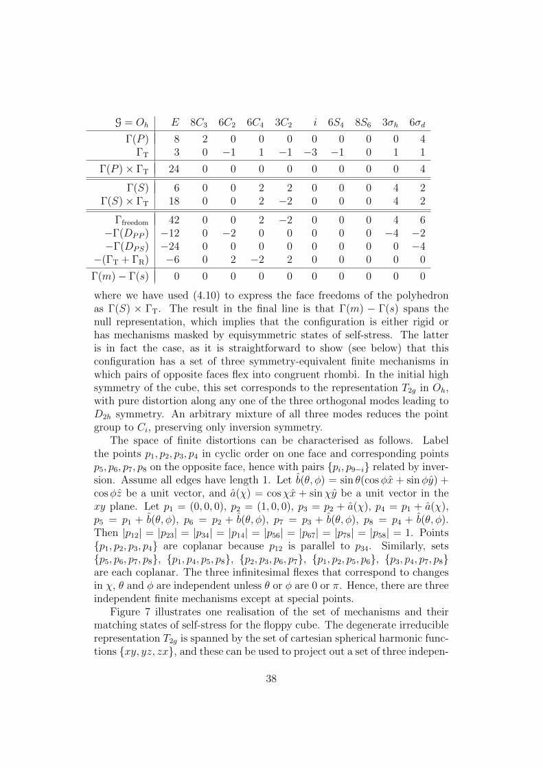
where we have used (4.10) to express the face freedoms of the polyhedronas Γ(S) × ΓT. The result in the final line is that Γ(m) − Γ(s) spans thenull representation, which implies that the configuration is either rigid orhas mechanisms masked by equisymmetric states of self-stress. The latteris in fact the case, as it is straightforward to show (see below) that thisconfiguration has a set of three symmetry-equivalent finite mechanisms inwhich pairs of opposite faces flex into congruent rhombi. In the initial highsymmetry of the cube, this set corresponds to the representation T2g in Oh,with pure distortion along any one of the three orthogonal modes leading toD2h symmetry. An arbitrary mixture of all three modes reduces the pointgroup to Ci, preserving only inversion symmetry.

The space of finite distortions can be characterised as follows. Labelthe points p1, p2, p3, p4 in cyclic order on one face and corresponding pointsp5, p6, p7, p8 on the opposite face, hence with pairs {pi, p9−i} related by inver-sion. Assume all edges have length 1. Let b(θ, φ) = sin θ(cosφx + sinφy) +cosφz be a unit vector, and a(χ) = cosχx + sinχy be a unit vector in thexy plane. Let p1 = (0, 0, 0), p2 = (1, 0, 0), p3 = p2 + a(χ), p4 = p1 + a(χ),p5 = p1 + b(θ, φ), p6 = p2 + b(θ, φ), p7 = p3 + b(θ, φ), p8 = p4 + b(θ, φ).Then |p12| = |p23| = |p34| = |p14| = |p56| = |p67| = |p78| = |p58| = 1. Points{p1, p2, p3, p4} are coplanar because p12 is parallel to p34. Similarly, sets{p5, p6, p7, p8}, {p1, p4, p5, p8}, {p2, p3, p6, p7}, {p1, p2, p5, p6}, {p3, p4, p7, p8}are each coplanar. The three infinitesimal flexes that correspond to changesin χ, θ and φ are independent unless θ or φ are 0 or π. Hence, there are threeindependent finite mechanisms except at special points.

Figure 7 illustrates one realisation of the set of mechanisms and theirmatching states of self-stress for the floppy cube. The degenerate irreduciblerepresentation T2g is spanned by the set of cartesian spherical harmonic func-tions {xy, yz, zx}, and these can be used to project out a set of three indepen-

38

z

xy

Figure 7: Equisymmetric flexes and states of self-stress for the ‘floppy cube’(with fixed edge lengths and planar faces). In the axis system defined onthe left, sets of independent flexes (top) and states of self-stress (bottom)transform as the coordinate products {xy, yz, zx}. For the flexes, arrowsindicate the direction of the initial displacement from the high-symmetryconfiguration; for the states of self-stress, inward/outward-pointing arrowsindicate tensile/compressive force.

dent flexes and corresponding states of self-stress. Flexes have displacementsin the planes of the maxima in the cartesian function; thus four cube facesrotate and two flex to make a rhombus. Each pattern of stresses involvesfour DPP constraints on the edges normal to the nominated cartesian plane,with an alternating cyclic pattern (+s,−s,+s,−s).

Point groups Oh, D2h, D3d, C2h and Ci are accessible in this distortionspace (figure 8). (See Guest and Fowler (2007), and also Jotham and Kettle(1971) where the same descent in symmetry is discussed for a problem inchemistry related to Jahn-Teller distortion in octahedral complexes.)

8 Mobility predictions for convex polyhedra

Simple counting of freedoms and constraints gives only the net mobility m−sand no conditions on the individual values of m and s. The symmetry-extended approach gives, in effect, a further set of necessary conditions on mand s, through determination of the difference Γ(m)−Γ(s), but again is notguaranteed to give full information on the separate representations Γ(m) andΓ(s). Symmetry often gives some added information through the pattern ofsigns in the reducible representation, giving partial but unambiguous contri-butions to Γ(m) and Γ(s). To take a concrete example, a count m − s = 0

39

Figure 8: Symmetries accessible in the T2g space of mechanisms of a cubewith fixed edge lengths and planar faces, illustrated with Polydron models.(Models consist of square plates and planar rhombi constructed from pairsof equilateral triangular plates.) The point groups are (left to right) Oh,D2h, C2h, D3d, with respectively 6, 4, 2, and 0 square, and 0, 2, 4, and 6rhomboidal faces.

shows that m and s are equal but not that they vanish individually. By thesame token, if computation leads to the conclusion that Γ(m) − Γ(s) is thenull representation, we know only that m−s and that the sets of mechanismsand states of self-stress are equisymmetric.

3D examples (a) to (d) include two cases where a cubic polyhedron underthe sole constraints of fixed edge lengths and planarity of faces turns out tohave the null representation for Γ(m) − Γ(s). We can generalise this resultto show that the mobility of any convex polyhedron under these constraintswill span the null representation, Γ(m)− Γ(s) = 0.

The proof follows a method used for deriving the symmetry extension ofthe Euler theorem (Ceulemans and Fowler, 1991). Let Γ(F ), Γ(E) and Γ(V )be the reducible representations for the permutations induced by symmetryelements of the group G on the sets of vertices, edges and faces of a poly-hedron, with characters χF (R), χE(R) and χV (R) equal to the numbers ofcomponents of each type that are unshifted under operation R ∈ G.

The case of the identity operation, R = E, is that of pure scalar counting.Suppose the polyhedron has f faces, e edges, and v vertices, and let face i haveni vertices. There are ni constraints of type DPS on the plane of face i and niedges on face i. We have Σini = 2e, as each edge is on two faces. Hence, wehave in total 3(f + v) freedoms, 2e constraints DPS and e constraints DPP

for our polyhedron with fixed-length edges and planar faces, and thus

F − C − 6 = 3(f + v − e− 2) = 0, (8.1)

by Euler’s theorem.Next, consider a rotation through a non-zero angle φ, i.e. the proper

40

rotation Cφ. We have Γfreedom = (Γ(P )+Γ(S))×ΓT. The axis of rotation mustpass through two structural elements of the polyhedron (vertex + vertex,vertex + edge midpoint, vertex + face centre, . . . , face centre + face centre).It may pass through an edge centre if φ = π. Let the number of faces, edgesand vertices intersected by a given Cφ axis be fφ, eφ and vφ, respectively, withfφ+eφ+vφ = 2, and let the character of the rigid-body translations be χT(Cφ)(with explicit formula χT(Cφ) = 1 + 2 cosφ and hence χT(Cφ) = −1 forφ = π). Then, for the character of the freedoms we have χfreedom(Cφ) = (fφ+vφ)χT(Cφ). For the edge constraints we have χPP (Cφ) = eφ = −eφχT(Cφ)as either φ = π or eφ = 0, or both. For the planarity constraints we haveχPS = 0 , as no vertex is at the centre of a face. Rigid-body motions giveχT(Cφ) + χR(Cφ) = 2χT(Cφ). Hence, in total we have

χm−s(Cφ) = (fφ + vφ)χT(Cφ) + eφ × χT(Cφ)− 2χT(Cφ) = 0. (8.2)

All faces, edges and vertices are shifted by inversion and rotation-reflections,so it remains only to consider a pure reflection, R = σ. A mirror plane inter-sects the shell in a loop of linked intersection elements of at most four types(Ceulemans and Fowler, 1991). These are shown as (i) to (iv) in Figure 9.Counting contributions, using half weighting for edges or vertices shared be-tween two intersected elements, gives

Character (i) (ii) (iii) (iv)

χS(σ) 1 1 1 0χP (σ) 0 1

212

+ 12

12

+ 12

−χDPP(σ) −(1

2+ 1

2) −1

20 −1

−χDPS(σ) 0 −1 −2 0

−χT(σ)− χR(σ) 0 0 0 0

χm−s(σ) 0 0 0 0

which shows that χm−s(σ) sums to zero over the whole loop for every reflec-tion plane. Hence, Γ(m) − Γ(s) = 0 for all polyhedra subject only to fulledge-length and face-planarity constraints.

As we have seen, vanishing of the mobility representation does not excludethe possibility of undetected mechanisms. The example of the cube sug-gests an infinite family of polyhedra with such mechanisms: any polyhedronconstructed by extrusion of a polygon, i.e. formed by joining correspondingvertices of two parallel congruent copies of polygons, will have all those mech-anisms that derive from in-phase combinations of the 2D mechanisms of theparallel polygons (if the polygons are of size greater than 3). Prisms form asubclass of extruded polyhedra. For the cube, the extrusion can be consid-ered to have happened in any one of three independent directions, hence thethreefold nature of the mechanism.

41

(i) (ii) (iii) (iv)

Figure 9: Intersection of a reflection plane with structural elements of a poly-hedron (Ceulemans and Fowler, 1991). See text for details of the calculationof their contributions to the mobility representation.

9 A note on freedoms of a cubic polyhedral

cage

The general symmetry-extended treatment can often be taken further inspecific situations. One such specialisation, which is of interest in severalcontexts, from CAD to structural mechanics and molecular force fields inphysical chemistry, is based on the family of cubic polyhedral cages. In aCAD context, a polyhedron can be considered as an assemblage of point,line and plane geometries. The polyhedral cages have rings of vertices andedges in place of solid faces, and these rings are not necessarily planar. Herewe concentrate on the freedoms of edges and vertices. From (4.1), (4.3), and(4.9), replacing P and L by v and e, respectively, these are:

vertices : Γ(v)× ΓT, (9.1)

edges : Γ(e)× (ΓT + ΓR)− Γ‖(e)× (Γ0 + Γε), (9.2)

For the object as a whole, rigid-body motions are accounted for by subtrac-tion of one copy of (ΓT + ΓR).

The sets of freedoms are not independent for a polyhedral object, as theEuler theorem and its symmetry-adapted counterpart apply, with significantconsequences, as illustrated here for cubic polyhedra. We can give physicalinterpretations to the freedom equations and their differences. One suchdifference is relevant to the construction of force fields for cubic polyhedralmolecular cages.

A set of edges, given full line freedoms, will simply drift apart. Therepresentation Γfreedom(e) must be reduced by some constraint Γev to produceΓ(v)×ΓT, the mechanical freedoms of the polyhedral cage. The constraint isthat at each vertex of a cubic polyhedron the three incident edges must havea common intersection and therefore must satisfy three pairwise intersectionconstraints of type DLL0.

42

We can show that these constraints correspond to a rotational triple ateach vertex, and hence span

Γev = Γfreedom(e)− Γfreedom(v) = Γ(v)× ΓR = Γ(v)× ΓT × Γε. (9.3)

The proof is straightforward. Expansion of Γev using (4.3) and (4.1) gives

Γev = Γ(e)× (ΓT + ΓR)− Γ‖(e)× (Γ0 + Γε)− Γ(v)× ΓT, (9.4)

and this can be simplified using the identities

Γ(e)× ΓT = Γ(e) + Γ‖(e) + Γ⊥(e), (9.5)

Γ‖(e) = Γ⊥(e)× Γε, (9.6)

and a specific consequence for cubic polyhedra of the symmetry-extendedEuler theorem (Ceulemans and Fowler, 1991),

Γ(v)× ΓT = Γ(e) + Γ‖(e), (9.7)

to give Γev as a function of edge representations, which collapses down to

Γev = Γ(e)× Γε + Γ⊥(e) = Γ(v)× ΓT × Γε = Γ(v)× ΓR. (9.8)

Hence, (9.3) is proved.The combination Γ(v)×ΓR also arises in other contexts. For example, in

Guest et al. (2018) it appears as the symmetry spanned by extra states of self-stress in a panel-hinge description of the net mobility of a fully triangulatedpolyhedron (‘extra’ compared to the isostatic bar-and-joint model). As alsoin the present application, the key point is that hinge lines (edges) associatedwith panels (or faces) around each polyhedral vertex meet at that commonvertex.

The identity (9.7) expresses the under-appreciated fact that the vibra-tional motions of a cubic polyhedral molecular framework can be expressedas a combination of bond stretches and ‘bond slides’ only, giving a basis fora novel type of force field for polyhedral cage molecules (Ceulemans et al.,2001).

10 Conclusions

A general symmetry extension of counting rules for CAD systems has beenderived. Symmetry extensions of counting arguments are useful in many spe-cific cases for deciding local redundancy of constraints, residual freedoms of

43

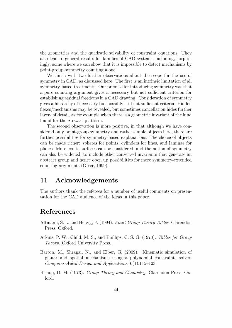
the geometries and the quadratic solvability of constraint equations. Theyalso lead to general results for families of CAD systems, including, surpris-ingly, some where we can show that it is impossible to detect mechanisms bypoint-group-symmetry counting alone.

We finish with two further observations about the scope for the use ofsymmetry in CAD, as discussed here. The first is an intrinsic limitation of allsymmetry-based treatments. Our premise for introducing symmetry was thata pure counting argument gives a necessary but not sufficient criterion forestablishing residual freedoms in a CAD drawing. Consideration of symmetrygives a hierarchy of necessary but possibly still not sufficient criteria. Hiddenflexes/mechanisms may be revealed, but sometimes cancellation hides furtherlayers of detail, as for example when there is a geometric invariant of the kindfound for the Stewart platform.

The second observation is more positive, in that although we have con-sidered only point-group symmetry and rather simple objects here, there arefurther possibilities for symmetry-based explanations. The choice of objectscan be made richer: spheres for points, cylinders for lines, and laminae forplanes. More exotic surfaces can be considered, and the notion of symmetrycan also be widened, to include other conserved invariants that generate anabstract group and hence open up possibilities for more symmetry-extendedcounting arguments (Olver, 1999).

11 Acknowledgements

The authors thank the referees for a number of useful comments on presen-tation for the CAD audience of the ideas in this paper.

References

Altmann, S. L. and Herzig, P. (1994). Point-Group Theory Tables. ClarendonPress, Oxford.

Atkins, P. W., Child, M. S., and Phillips, C. S. G. (1970). Tables for GroupTheory. Oxford University Press.

Barton, M., Shragai, N., and Elber, G. (2009). Kinematic simulation ofplanar and spatial mechanisms using a polynomial constraints solver.Computer-Aided Design and Applications, 6(1):115–123.

Bishop, D. M. (1973). Group Theory and Chemistry. Clarendon Press, Ox-ford.

44

Bouma, W., Fudos, I., Hoffmann, C., Cai, J., and Paige, R. (1995). GeometricConstraint Solver. Computer-aided Design., 27(6):487–501.

Calladine, C. R. (1978). Buckminster Fuller’s “Tensegrity” structures andClerk Maxwell’s rules for the construction of stiff frames. InternationalJournal of Solids and Structures, 14:161–172.

Ceulemans, A. and Fowler, P. W. (1991). Extension of Euler’s theorem tothe symmetry properties of polyhedra. Nature, 353:52–54.

Ceulemans, A., Titeca, B. C., Chibotaru, L. F., Vos, I., and Fowler, P. W.(2001). Complete bond force fields for trivalent and deltahedral cages:group theory and applications to cubane, closo-dodecaborane and buck-minsterfullerene. Journal of Physical Chemistry A, 105:8284–8295.

Fowler, P. W. and Guest, S. D. (2000). A symmetry extension of Maxwell’srule for rigidity of frames. International Journal of Solids and Structures,37:1793–1804.

Fowler, P. W. and Guest, S. D. (2005). A symmetry analysis of mecha-nisms in rotating rings of tetrahedra. Proceedings of the Royal Society:Mathematical, Physical & Engineering Sciences, 461:1829–1846.

Fowler, P. W. and Quinn, C. M. (1986). σ, π and δ representations of themolecular point groups. Theoretica Chimica Acta, 70(5):333–350.

Griffith, J. S. (2009). The Theory of Transition-Metal Ions. CambridgeUniversity Press.

Guest, S. D. and Fowler, P. W. (2005). A symmetry-extended mobility rule.Mechanism and Machine Theory, 40:1002–1014.

Guest, S. D. and Fowler, P. W. (2007). Symmetry conditions and finitemechanisms. Journal of Mechanics of Materials and Structures, 2(2):293–301.

Guest, S. D., Fowler, P. W., and Schulze, B. (2018). Mobility of symmetricblock-and-hole polyhedra. International Journal of Solids and Structures,150:40–51.

Guest, S. D., Schulze, B., and Whiteley, W. J. (2010). When is a body-bar structure isostatic? International Journal of Solids and Structures,47:2745–2754.

45

Jackson, B. and Owen, J. C. (2016). A characterisation of the generic rigidityof 2-dimensional point-line frameworks. Journal of Combinatorial Theory,Series B, 119:96–121.

Jackson, B. and Owen, J. C. (2019). Radically solvable graphs. Journal ofCombinatorial Theory, Series B, 136:135–153.

Jotham, R. W. and Kettle, S. F. A. (1971). Geometrical consequences of theJahn-Teller effect. Inorganica Chimica Acta, 5:183–187.

Kangwai, R. D. and Guest, S. D. (1999). Detection of finite mechanismsin symmetric structures. International Journal of Solids and Structures,36(36):5507–5527.

Kim, K., Lee, J. Y., and Kim, K. (1998). A 2-D geometric constraint solverusing dof-based graph reduction. Computer-aided Design., 30(11):883–896.

Klein, F. (1870). Zur theorie der liniencomplexe des ersten und zweitengrades. Math. Ann., 2:198–226.

Maxwell, J. C. (1864). On the calculation of the equilibrium and stiffness offrames. Philosophical Magazine., 27:294–299.

Muller, A. (2016). Recursive higher-order constraints for linkages with lowerkinematic pairs. Mechanism and Machine Theory, 100:33–43.

Nawratil, G. (2013). Types of self-motions of planar Stewart–Gough plat-forms. Meccanica, 48:1177–1190.

Olver, P. J. (1999). Equivalence, Invariants and Symmetry. London Mathe-matical Society Lecture Notes, Cambridge University Press.

Owen, J. C. (1991). Algebraic solution for geometry from dimensional con-straints. In Proceedings of the First ACM Symposium on Solid ModelingFoundations and CAD/CAM Applications, SMA ’91, pages 397–407, NewYork, NY, USA. ACM.

Owen, J. C. and Power, S. C. (2006). The non-solvability by radicals ofgeneric 3-connected planar Laman graphs. Transactions of the AmericanMathematical Society, 359:2269–2303.

Owen, J. C. and Power, S. C. (2010). Framework symmetry and rigidity. In-ternational Journal of Computational Geometry and Applications, 20:723–750.

46

Plucker, J. (1865a). I. on a new geometry of space. Proceedings of the RoyalSociety of London, 14:53–58.

Plucker, J. (1865b). Xvii. on a new geometry of space. Philosophical Trans-actions of the Royal Society of London, 155:725–791.

Quinn, C. M., McKiernan, J. G., and Redmond, D. B. (1984). Mollweideprojections and symmetries on the spherical shell. Jounal of ChemicalEducation, 61:569–571 and 572–579.

Schulze, B. (2010). Symmetry as a sufficient condition for a finite flex. SIAMJournal on Discrete Mathematics, 24(4):1291–1312.

Sitharam, M., St. John, A., and Sidman, J., editors (2019). Handbook ofGeometric Constraint Systems. CRC Press.

Spivak, M. (1965). Calculus on manifolds. A modern approach to classi-cal theorems of advanced calculus. W. A. Benjamin, Inc., New York-Amsterdam.

47

Applications of symmetry in point-line-plane frameworks ...

Documents

Transcript of Applications of symmetry in point-line-plane frameworks ...