Applications of Space-Filling Curves to Cartesian Methods for CFD

M. J. Aftosmis

†

Mail Stop T27B NASA Ames Research Center

Moffett Field, CA 94404

aftosmis@nas.nasa.gov

M. J. Berger

‡

Courant Institute251 Mercer St.

New York, NY 10012

berger@cims.nyu.edu

S. M. Murman

¥

ELORETNASA Ames Research Center

Moffett Field, CA 94404

smurman@nas.nasa.gov

This paper presents a variety of novel uses of space-filling curves (SFCs) for Cartesian meshmethods in CFD. While these techniques will be demonstrated using non-body-fitted Cartesianmeshes, many are applicable on general body-fitted meshes – both structured and unstructured. Wedemonstrate the use of single

O

(

N

log

N

) SFC-based reordering to produce single-pass (

O

(

N

)) algo-rithms for mesh partitioning, multigrid coarsening, and inter-mesh interpolation. The intermeshinterpolation operator has many practical applications including “warm starts” on modified geome-try, or as an inter-grid transfer operator on remeshed regions in moving-body simulations. Exploitingthe compact construction of these operators, we further show that these algorithms are highly amena-ble to parallelization. Examples using the SFC-based mesh partitioner show nearly linear speedup to640 CPUs even when using multigrid as a smoother. Partition statistics are presented showing that theSFC partitions are, on-average, within 15% of ideal even with only around 50,000 cells in each sub-domain. The inter-mesh interpolation operator also has linear asymptotic complexity and can be usedto map a solution with

N

unknowns to another mesh with

M

unknowns with

O

(

M + N

) operations.This capability is demonstrated both on moving-body simulations and in mapping solutions to per-turbed meshes for control surface deflection or finite-difference-based gradient design methods.

42

ND

A

EROSPACE

S

CIENCES

M

EETING

AND

E

XHIBIT

R

ENO

N

EVADA

, 5-8 J

ANUARY

2004

AIAA-2004-1232

1 Introduction HE literature on numerical methods for Partial Differen-tial Equations (PDEs) contains a wealth of diverse

approaches for improving cache performance, performingdomain decomposition, mesh coarsening and inter-meshsolution transfer. The infrastructure and algorithms support-ing these operations are frequently unrelated and usuallyrequire different data structures and infrastructure to performeach task. For example, a high-performance, distributed-memory, unstructured mesh code may use Reverse Cuthill-McKee (RCM) ordering for improving cache-performance,recursive spectral bisection, or multi-level nested dissectionfor domain decomposition,[1][2] a graph-based meshcoarsener[4][3] and variety of fast spatial search data struc-tures for inter-mesh interpolation, or solution transfer to re-gridded regions of a subdomain.

For each task, these techniques offer superb performance,and many of them are amenable to some degree of parallel-ization. Nevertheless, development and maintenance of sucha diverse collection of tools requires considerable investment,and when a substantial overhaul is necessary (e.g. moving acode to distributed-memory parallelization) the level of effortrequired will be significant.

Space-filling curves (SFCs) offer a unifying data structure forall of these ends. Construction of these curves is extremelyinexpensive as the SFC index for any voxel in space may becomputed using only local information, and thus computa-tion of indices may be performed in parallel. The asymptotic

time complexity of constructing the curve is thereforebounded by the sort algorithm which orders the mesh alongthe curve. This sort can be performed with standard sortingroutines such as quicksort which produces a method withO(N log N) running time. After this initial sort, all subsequentcoarsening, decomposition, and interpolation can may beperformed with linear sweeps through the reordered mesh.

2 Space-Filling CurvesThe central operation in using space-filling curves is a reor-dering of the mesh using one of the dozens of well-docu-mented space-filling curves. In this work we consider boththe Morton and Peano-Hilbert order[6]. Both orderings havebeen explored in scientific computing in a variety of roles,including the parallel solution of N-body problems in compu-tational physics[7], algebraic multigrid[8], mesh generation,[9]

in the solution of PDEs and dynamic repartitioning of adap-tive methods[10]. Figure 1 shows both Peano-Hilbert andMorton SFCs constructed on Cartesian meshes at three levelsof refinement. In two dimensions, the basic building block ofthe Hilbert curves is a “U” shaped line which visits each of 4cells in a 2 x 2 block. Each subsequent level further dividesthe previous level’s cells, creating subquadrants which are,themselves, visited by (rotated) U shaped curves as well.Similar properties exist for the Morton ordering which usesan “N” shaped curve as its basic building block.

In three spatial dimensions the curves follow the same basicconstruction rules, but the basic building block extends intothe third dimension with additional U or N-shaped turns. Fig-ure 2 illustrates this 3-D construction for the U-order show-ing: (a) the basic 2x2x2 building block (b) the same meshafter one uniform refinement, where each segment of thecurve is replaced with an appropriately rotated basic building

† Research Scientist, Senior Member AIAA‡ Professor, Member AIAA¥ Senior Research Scientist, Member AIAA.

This material is declared a work of the U.S. Government and is not subject to copy-right protection in the United States.

T

AIAA 2004-1232 – 42

ND

AIAA A

EROSPACE

S

CIENCES

M

EETING

AND

E

XHIBIT

block, (c) the curve after additional adaptive refinement ofcells near the back-south-west corner. Properties and d-dimensional construction rules for these space-filling curvesare discussed extensively in refs. [11], [12] and [13].

Both orderings have locality properties which make themattractive as mesh partitioners[10][9]. For the present, we noteonly that such orderings have 3 important properties.

1. Mapping : The U and N orderings eachprovide unique mappings from the d-dimensionalphysical space of the problem domain Rd to a one-dimensional hyperspace, U, which one traverses fol-lowing the curve.

2. Locality: In the U-order, each cell visited by thecurve is directly connected to two face-neighboringcells which remain face-neighbors in the one dimen-sional hyperspace spanned by the curve. Locality inN-ordered domains is almost as good[6].

3. Compact Construction: Encoding and decoding theHilbert or Morton order requires only local informa-tion. Following the integer indexing for Cartesianmeshes outlined in ref. [5], a cell’s 1-D index in Umay be constructed using only that cell’s integer coor-dinates in Rd and the maximum number of refine-ments that exist in the mesh. This aspect is in markedcontrast to other partitioning schemes based on recur-sive spectral bisection or other multilevel decomposi-tion approaches which require the entire connectivitymatrix of the mesh in order to perform the partition-ing.

To illustrate the compact construction rules for these order-ings, consider the position of a cell i in the N-order. One wayto construct this mapping would be from a global operationsuch as a recursive lexicographic ordering of all cells in thedomain. Such a construction would not satisfy the propertyof compactness. Instead, the index of i in the N-order may bededuced solely by inspection of cell i’s integer coordinates(xi, yi, zi).

Assume is the bitwise representation of the integercoordinates (xi, yi, zi) using m-bit integers. The bit sequence

denotes a 3-bit integer constructed by interleavingthe first bit of xi, yi and zi. One can then immediately com-pute cell i’s location in U as the 3m-bit integer

. Thus, simply by inspection of acell’s integer coordinates, we are able to directly calculate its

Figure 1: Space-filling curves used to order three Cartesianmeshes in two spatial dimensions: a) Peano-Hilbert or “U-ordering”, b) Morton or “N-ordering”.

a)

b)

a.

b.

c.

Figure 2: U-order in three dimensions for (a) a basic 2x2x2block of cells, (b) the same block after uniform subdivision(c) cell order after refinement near the south-west-back cor-

M : R d U →

Figure 3: Morton order of an adaptively refined Cartesian mesharound a 2-D airfoil.

xi yi zi, ,( )

xi1yi

1zi

1{ }

xi1yi

1zi1xi

2yi2zi

2…ximyi

mzim{ }

2 OF 12

AIAA 2004-1232 – 42ND AIAA AEROSPACE SCIENCES MEETING AND EXHIBIT

location,

M

(

i

), in the one-dimensional space

U

without anyadditional information. Similarly compact construction rulesexist for the U-order

[13]

.

In an h -refined Cartesian mesh, the finest cell can be used todefine the dimensions of a single voxel

1. All coarser cells

may then be reinterpreted as collections of this basic buildingblock and are referred to by the index of their lowest constit-uent voxel. This interpretation leads to an integer indexingscheme which can be used to address all cells in the computa-tional domain. With this integer indexing scheme, the con-struction rules in the previous paragraph can then be appliedto generate the Morton index, M(i), of all the cells in themesh. Figure 3 shows an example of the N-ordering on anadaptively refined mesh around a 2-D airfoil.

Construction of the Peano-Hilbert index, H(i), follows a sim-ilarly compact procedure. After computing the SFC indicesM(i) or H(i) for all the cells in the mesh, one simply takesthese indices as sort keys and applies any one of the standardsorting algorithms (we use the quicksort algorithm from theC standard library). Since all the other data required for con-struction is local, the sort establishes the asymptotic boundfor runtime of the reordering and choosing quicksort givestypical runtimes of O(N log N). In more concrete terms, com-puting M(i) and H(i) and then sorting cells and faces takesunder 4 seconds per million cells on a 2Ghz Pentium 4.

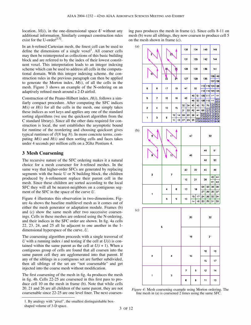
3 Mesh CoarseningThe recursive nature of the SFC ordering makes it a naturalchoice for a mesh coarsener for h-refined meshes. In thesame way that higher-order SFCs are generated by replacingsegments with the basic U or N building block, the childrenproduced by h-refinement replace their parent cell in themesh. Since these children are sorted according to the localSFC they will all be nearest-neighbors on a contiguous seg-ment of the SFC in the space of the curve U.

Figure 4 illustrates this observation in two-dimensions. Fig-ure 4a shows the baseline multilevel mesh as it comes out ofeither the mesh generator or adaptation module. Frames (b)and (c) show the same mesh after two successive coarsen-ings. Cells in these meshes are ordered using the N-ordering,and their indices in the SFC order are shown. In fig. 4a cells22, 23, 24, and 25 all lie adjacent to one another in the 1-dimensional hyperspace of the curve, U.

The coarsening algorithm proceeds with a single traversal ofU with a running index i and testing if the cell at U(i) is con-tained within the same parent as the cell at U(i + 1). When acontiguous group of cells are found that all coarsen into thesame parent cell they are agglomerated into that parent. Ifany of the siblings in a contiguous set are further subdivided,then all siblings of the set are “not coarsenable” and getinjected into the coarse mesh without modification.

The first coarsening of the mesh in fig. 4a produces the meshin fig. 4b. Cells 22-25 are coarsened in this first pass to pro-duce cell 10 on the mesh in frame (b). Note that while cells20, 21 and 26 are all children of the same parent, they are notcoarsenable since 22-25 are one level finer. The next coarsen-

ing pass produces the mesh in frame (c). Since cells 8-11 onmesh (b) were all siblings, they now coarsen to produce cell 5on the mesh shown in frame (c).

Figure 4: Mesh coarsening example using Morton ordering. Thefine mesh in (a) is coarsened 2 times using the same SFC.

(c)

(b)

(a)

3 OF 12

1. By analogy with “pixel”, the smallest distinguishable box-shaped volume of 3-D space.

AIAA 2004-1232 – 42

ND

AIAA A

EROSPACE

S

CIENCES

M

EETING

AND EXHIBIT

Figure 5 shows an example in three dimensions. In thisexample, a 4.5M cell adaptively-refined mesh around twosurface ships has undergone 4 cycles of coarsening byagglomeration along the SFC. The final mesh shown in thelower right frame of the figure contains 4500 cells. In prac-tice, typical coarsening ratios for the algorithm are in excessof 7 on realistically complex problems.[16]

4 Domain decompositionThe mapping and locality properties that are exploited for thesingle-pass mesh coarsener described above make SFCs anatural choice for partitioners on hierarchicalmeshes.[8][9][15][16] Figure 6 illustrates these mapping andlocality properties for an adapted two-dimensional Cartesianmesh, partitioned into three subdomains. The figure pointsout that for adapted Cartesian meshes, the hyperspace U maynot be fully populated by cells in the mesh.

The quality of the partitioning resulting from U-orderedmeshes have been examined in ref. [10] and were found to be

competitive with respect to other popular partitioners.Weights can be assigned on a cell-by-cell basis. One advan-tage of using this partitioning strategy stems from the obser-vation that mesh refinement or coarsening simply increasesor decreases the population of U while leaving the relativeorder of elements away from the adaptation unchanged. Re-mapping the new mesh into new subdomains therefore onlymoves data at partition boundaries and avoids global remap-pings when cells adaptively refine during mesh adaptation.Recent experience with a variety of global repartitioners sug-gest that the communication required to conduct this remap-ping can be an order of magnitude more expensive than therepartitioning itself[14]. Additionally, since the partitioner justinserts breaks into the U-ordered cell list on-the-fly, the entiremesh may be stored as a single domain. At run-time, this sin-gle mesh may then be partitioned into any number of subdo-mains as it is read into the flow solver from mass storage.One benefit of this approach is that a simulation begun onsome given number of CPUs may be restarted on a differentnumber of CPUs. Alternatively, when performing parameterstudies on a fixed mesh, each simulation may be run on a dif-ferent number of CPUs - all sharing the same copy of theinput mesh file. In a heterogeneous shared timesharing envi-ronment, where the number of available processors may notbe known at the time of job submission, the value of suchflexibility is obvious.

The SFC reordering pays additional dividends in cache-per-formance. The locality property of the SFC produces a con-nectivity matrix which is tightly clustered regardless of thenumber of subdomains. Our numerical experiments suggestthat SFC reordered meshes have about the same data cachehit-rate as those reordered using reverse Cuthill-McKee.

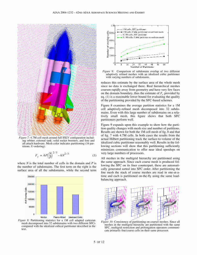
Figure 7 shows an example of a three dimensional Cartesianmesh around the full Space Shuttle Launch Vehicle (SSLV)configuration. This complex configuration includes theorbiter, external tank, solid rocket boosters, and fore and aftattach hardware. The computational mesh contains about4.7M cells at 14 levels of refinement, and is indicated by asingle cutting plane passed through the mesh just behind theSSLV geometry. The coloring of gridlines in the mesh showsits partitioning into 16 subdomains using the U-order. Reor-dering this mesh with the algorithm of §2 required 20 sec. ona 2 Ghz Pentium 4, and preparing 4 levels of coarser meshesfor multigrid required 15 sec. on the same machine. Partitionboundaries are chosen to balance the load in each subdomain.In determining work loads, cut-cells were weighted 2.1x ascompared to un-cut Cartesian hexahedra.

The partitioning in fig. 7 demonstrates how, even on adap-tively-refined meshes, the partitioning tends to produce sub-domains that are largely rectilinear. On a uniform mesh, anappropriately chosen number of partitions would result in acubical decomposition of the computational domain. This“best case” establishes the minimum ratio of communicationto computation (surface/volume ratio) for SFC partitionedmeshes. For any given number of cells, one can conceive ofan idealized cubical partitioner which would communicateacross some number of faces, Fc given by:

Figure 5: Mesh coarsening example in 3D using agglomerationalong the SFC. The finest mesh contains 4.5M cells while thecoarsest contains 4500 cells after 4 coarsenings.

a

b

c

d

ef

g h

i j

k

lm

n o

pq

r

s

part 1

part 2

part 3

2-D physical space

1-D hyperspace

a b c d e f g hi j k lmnop q r s

part 1 part 2 part 3

Figure 6: An adapted Cartesian mesh and associated space-fillingcurve based on the U-ordering of with the U-ordering illustrating locality and mesh partitioning in two spa-tial dimensions. Partitions are indicated by the heavy dashedlines in the sketch.

M : R d U →

4 OF 12

AIAA 2004-1232 – 42ND AIAA AEROSPACE SCIENCES MEETING AND EXHIBIT

(1)

where

N

is the total number of cells in the domain and

P

isthe number of subdomains. The first term on the right is thesurface area of all the subdomains, while the second term

reduces this estimate by the surface area of the whole meshsince no data is exchanged there. Real hierarchical meshescoarsen rapidly away from geometry and have very few faceson the domain boundary, thus the estimate of

F

c

provided byeq. (1) is a reasonable lower bound for evaluating the qualityof the partitioning provided by the SFC-based schemes.

Figure 8 examines the average partition statistics for a 1Mcell adaptively-refined mesh decomposed into 32 subdo-mains. Even with this large number of subdomains on a rela-tively small mesh, this figure shows that both SFCpartitioners perform well.

Figure 9 expands upon this example to show how the parti-tion quality changes with mesh size and number of partitions.Results are shown for both the 1M cell mesh of fig. 8 and thatof fig. 7 with 4.7M cells. In both cases the results from theactual Hilbert partitioning track the surface-to-volume of theidealized cubic partitioner reasonably well. Results in the fol-lowing sections will show that this partitioning sufficientlyminimizes communication to offer near ideal speedups onvery large numbers of processors.

All meshes in the multigrid hierarchy are partitioned usingthe same approach. Since each coarse mesh is produced fol-lowing the SFC on its finer counterpart, these are automati-cally generated sorted into SFC order. After partitioning thefine mesh the stack of coarse meshes are read in one-at-a-time and each is partitioned on-the-fly using the same load-balancing approach.

Fc 6PNP---- 2 3⁄

6N2 3⁄

–=

Figure 7: 4.7M cell mesh around full SSLV configuration includ-ing orbiter, external tank, solid rocket boosters, and fore andaft attach hardware. Mesh color indicates partitioning (16 par-titions, U-ordering).

Figure 8: Partitioning statistics for a 1M cell adapted cartesianmesh decomposed into 32 subdomains with two different SFCscompared with the idealized cubical partitioner described in thetext.

Figure 9: Comparison of subdomain overlap of two differentadaptively refined meshes with an idealized cubic partitionerwith varying numbers of subdomains.

Figure 10: Consistency of partitioning on coarser meshes. Since allmeshes in the multigrid hierarchy are partitioned with the sameSFC, multigrid restriction and prolongation operators communi-cate primarily fine/coarse cells on their same processor.

5 OF 12

AIAA 2004-1232 – 42ND AIAA AEROSPACE SCIENCES MEETING AND EXHIBIT

In most graph-based approaches to mesh partitioning, repar-titioning the coarse mesh offers no guarantee of good overlapbetween coarse and fine partitions sitting on any given pro-cessor. Since the intergrid transfer operators in multigridintroduce communication between

every

cell

in successivemeshes in the hierarchy, good overlap limits the amount ofoff-processor bandwidth required for intergrid transfer. WithSFC partitioned meshes, all meshes are being partitioned byexactly the same SFC, uniformly coarsened meshes wouldhave maximal overlap with their finer counterparts. In prac-tice, the coarsening is modified by refinement boundaries andcoarsening rules, but uniform coarsening remains a goodmodel. Figure 10 demonstrates this by showing the coarsen-ing of a multilevel Cartesian mesh around a reentry vehicle.For simplicity, the mesh is shown partitioned into 2 subdo-mains. The subdomain boundaries in this example show goodconsistency of partitioning and 96% of the cells on the finestmesh restrict to coarser cells residing on the same processor.Only 4% of the communication for intergrid transfer needs togo between processors.

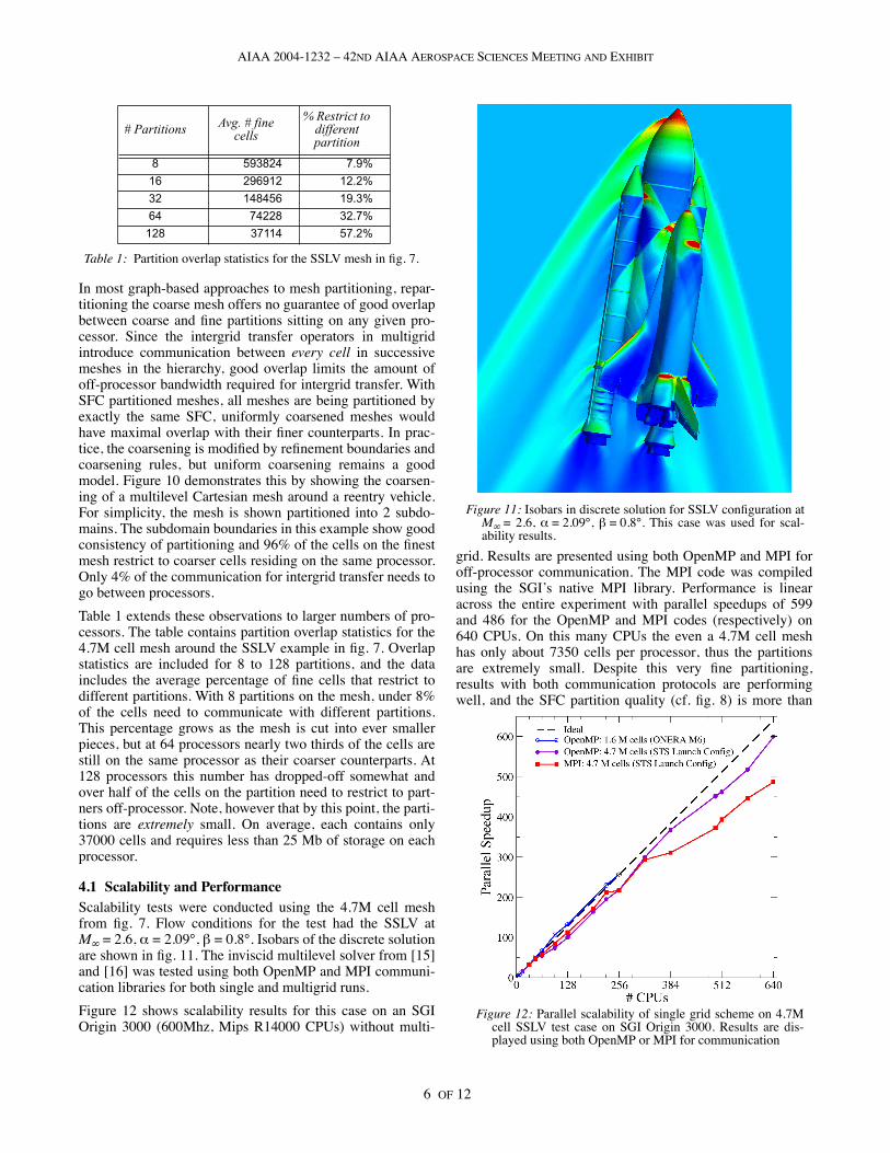
Table 1 extends these observations to larger numbers of pro-cessors. The table contains partition overlap statistics for the4.7M cell mesh around the SSLV example in fig. 7. Overlapstatistics are included for 8 to 128 partitions, and the dataincludes the average percentage of fine cells that restrict todifferent partitions. With 8 partitions on the mesh, under 8%of the cells need to communicate with different partitions.This percentage grows as the mesh is cut into ever smallerpieces, but at 64 processors nearly two thirds of the cells arestill on the same processor as their coarser counterparts. At128 processors this number has dropped-off somewhat andover half of the cells on the partition need to restrict to part-ners off-processor. Note, however that by this point, the parti-tions are

extremely

small. On average, each contains only37000 cells and requires less than 25 Mb of storage on eachprocessor.

4.1 Scalability and Performance

Scalability tests were conducted using the 4.7M cell meshfrom fig. 7. Flow conditions for the test had the SSLV at

M

∞

= 2.6,

α

= 2.09°,

β

= 0.8°. Isobars of the discrete solutionare shown in fig. 11. The inviscid multilevel solver from [15]and [16] was tested using both OpenMP and MPI communi-cation libraries for both single and multigrid runs.

Figure 12 shows scalability results for this case on an SGIOrigin 3000 (600Mhz, Mips R14000 CPUs) without multi-

grid. Results are presented using both OpenMP and MPI foroff-processor communication. The MPI code was compiledusing the SGI’s native MPI library. Performance is linearacross the entire experiment with parallel speedups of 599and 486 for the OpenMP and MPI codes (respectively) on640 CPUs. On this many CPUs the even a 4.7M cell meshhas only about 7350 cells per processor, thus the partitionsare extremely small. Despite this very fine partitioning,results with both communication protocols are performingwell, and the SFC partition quality (cf. fig. 8) is more than

Table 1: Partition overlap statistics for the SSLV mesh in fig. 7.

# Partitions Avg. # fine cells

% Restrict to different partition

8 593824 7.9%

16 296912 12.2%

32 148456 19.3%

64 74228 32.7%

128 37114 57.2%

Figure 11: Isobars in discrete solution for SSLV configuration atM∞ = 2.6, α = 2.09°, β = 0.8°. This case was used for scal-ability results.

Figure 12:

Parallel scalability of single grid scheme on 4.7M

cell SSLV test case on SGI Origin 3000. Results are dis-played using both OpenMP or MPI for communication

6 OF 12

AIAA 2004-1232 – 42ND AIAA AEROSPACE SCIENCES MEETING AND EXHIBIT

adequate on this computing platform. To reiterate this point,the plot also shows results for a 1.6M cell mesh distributedonto as many as 256 processors (~6250 cells/partition). Thiscurve lays on top of the “ideal” curve over its entirety. Theslight performance advantage shown by OpenMP is probablydue to the additional time required in the MPI code to explic-itly pack and unpack the messages passed between partitions.All scalability runs were conducted with the machine in non-dedicated mode (normal queuing system), and its expectedthat some of the irregularity in the curves would improveunder dedicated usage.

Figure 13 shows a similar scalability study using 3-level mul-tigrid (W-cycles) using the same test cases. The additionalcommunication load due to off-processor intergrid transferpointed to by Table 1 starts to become apparent on large num-bers of processors. Nevertheless results are still quite good.The OpenMP code achieves parallel speedups of about 514on 640 CPUs while the MPI version shows about 392. Thefirst and second coarse meshes in this grid hierarchy have700000 and 105000 cells respectively. These translate intoaverage cell counts of only 1100 and 180 cells per partition.

5 Inter-mesh Interpolation

The problem of efficient transfer of solutions or residualsfrom one mesh to another comes up frequently in vehicleanalysis. In stability and control analysis, for example, onemay wish to “warm-start” a solution with a deflected controlsurface from some undeflected baseline solution. In designusing finite-difference-based gradients, it is common practiceto compute a baseline configuration and then perturb theshape to establish the gradients with respect to the shapechange. Since these perturbations are small, it makes sense tore-use the pre-computed baseline to warm-start the perturbedsolutions. In moving-body simulations, when the body hasmoved, the geometry is no longer the same and we are again

in a situation of needing to transfer the solution (and perhapsresidual) to a new, but nearby, mesh.

In general, cells in the new mesh do not have a one-to-onecorrespondence with cells in the old mesh and some sort ofthree dimensional interpolation is required. At worst, findinginterpolants may require searching over all the cells in themesh, and such brute force algorithms are not practical. With

N

cells in the old mesh and

M

cells in the new mesh, anyalgorithm that runs in

O

(

N M

) time is sure to be expensivewhen both

N

and

M

are 10

7

or 10

8

.

Even with parallelization and more sophisticated algorithms,inter-mesh transfer can be expensive. For example, Ref. [17]reports that finding interpolation coefficients on a 324000cell mesh required 200 seconds on 16 CPUs. Otherapproaches use binning, hashing or a variety of spatial treestructures to limit the exhaustive searching needed for findinginterpolation stencils

[18][19]

. Since these data structures arecreated for the interpolation, their construction cost (typically

O

(

N

log

N

)) must be included in the interpolation time.

SFCs offer an attractive alternative for performing this trans-fer. The key to this use is to recognize that for any Cartesianmeshes with the same bounding box and number of coarsedivisions, a single SFC describes all possible meshes cover-ing the space. Essentially the SFC is playing the same role asa spatial data structure that spatial trees or coordinate bisec-tion play in other approaches. An important difference is thatrather than sorting into bins or traversing trees, the SFC sortsthe meshes into a unique order visiting each cell only once ineach mesh. With both meshes sorted, mapping from one toanother becomes a simple task of walking down the SFCthrough both meshes in “lock step”, marking time in one orthe other as needed to accommodate nested refinement orboundaries.

Figure 14 provides a more concrete view of this using anexample where we wish to map the data from the red mesh(left) to the blue mesh (right). Both meshes are visited by thesame SFC. In the sketch, each cell is annotated with its SFCindex showing the order in which the mapping algorithmsweeps the mesh. Cells 1-4

red

and 1-4

blue

are identical (sameSFC index, and same size), so the current position countersfor each of the two meshes will get incremented symmetri-cally as we progress through these cells. Entering cell 5, wenote that 5

blue

is larger than 5

red

so the counter on the blue

Figure 13: Parallel scalability of 3-level multigrid scheme on4.7M cell SSLV test case on SGI Origin 3000. Results aredisplayed using both OpenMP or MPI for communication

1 2

34

5

6 7

8 9

1314

15 16 1 2

34

5 9

1314

15 16

10 11

12

Figure 14:

SFC used to map data from the red mesh (left) to theblue mesh (right).

7 OF 12

AIAA 2004-1232 – 42ND AIAA AEROSPACE SCIENCES MEETING

AND

E

XHIBIT

mesh will not get incremented until it encounters the next cellon the red mesh that is not contained. In this way we simplymark time on the blue mesh until we encounter 9red which isthe first cell not contained by 5blue. Data in 5-8red all getmapped to 5blue. 9red is the first uncontained cell and weimmediately notice that 9blue is smaller than 9red. This timeits the red counter that gets suspended while cells 9-12blue allreceive a prolongation of the data in 9red. Cells 13-16 matchone-to-one in both meshes and are filled by direct injection.

From this sketch of the algorithm several things are clear: (1)Counters in both meshes increment monotonically. (2) At ter-mination, both counters reach their respective maximums. (3)Every step of the algorithm increments counters in either thered, blue or both meshes. Thus if there are N cells in the redmesh, and there are M cells in the blue mesh, the algorithmhas a run-time complexity of O(N + M), provided that the redand blue meshes are already in SFC order. If the meshes arenot already sorted, the operation is bounded by theO(N log N) complexity of the reordering.

Figure 15 outlines the situation when the red or blue meshescontain internal geometry. In this situation, cells that arecompletely internal to the geometry do not appear in themeshes. This leaves a gap in the SFC indexing on the meshnot covered by the extent of any cell. In the figure, cells 1-7map one-to-one but there is a gap between 7red and 9red notcover by the size of 7red. Thus no map exists for 8blue. Cells9-11 map one-to-one, but 12red has no counterpart in the bluemesh. Since we are interested in generating a mapping fromblue to red, 8blue gets assigned a nomap flag, and 12red sim-ply gets skipped.

Figure 16 contains Algorithm M. with a detailed descriptionof the full mapping algorithm handling both mesh refinementand changes in geometry. This algorithm is couched as adriver loop over the blue mesh which recursively calls a map-ping function that increments counters in the red and bluemesh. Since it visits each cell in the red and blue meshesonce each, Alg. M. has run-time complexity of O(N + M)which is linear in the total number of cells on the red and bluemeshes - provided that both meshes are already sorted in SFCorder. The algorithm makes use of the same prolongation andrestriction operators as used by the multigrid scheme. Directinjection is used for prolongation of the flow state, while vol-ume weighted averages are used for restriction. Since themajority of the cells map either 1:1 or, as a coarsening/refine-ment, the tail-recursion in M4.1.1 is rarely exercised. The

current algorithm simplifies the implementation at a nominalrun-time cost. When the blue mesh encounters a region forwhich there is no mapping (due to a hole, or “solid” region,in the red mesh) it gets a NO_MAP flag. When used forrestarts, these nomaps are populated with freestream quanti-ties. In the case of time-dependent moving-body simulations,nomaps indicate a cell that was uncovered by the motion ofthe geometry over the timestep. In this case, the state vectoris set to zero, and the cell is filled by the space-time fluxes inthe moving-body scheme.

Since it is a linear-time procedure, Algorithm M typicallyruns in seconds, even on meshes containing several millioncells. Timing examples were run on a 2 Ghz Pentium 4 desk-top machine using meshes similar to the 4.7M SSLV caseused above. In these, tracing the space-filling curve withAlgorithm M takes about 0.5 seconds, and actually transfer-ring the state vector using this map takes about 1.5 seconds.Reordering cells and faces using the space-filling curve forsuch a mesh takes about 20 seconds, however this one-timecost was already paid during construction of the coarsemeshes on the receiving grid.

The real utility of the intergrid transfer comes when thegeometry is slightly modified and we seek a solution to anearby problem. Since Cartesian meshes are ridged, they donot distort to follow the moving geometry, but instead resultin a mesh with a different, but nearby, sets of cut, volume andinterior cells. Examples of this exist in design, control sur-face deflection, and moving body simulations.

1 2

34

5

67

9

1314

15 16

10 11

12

1 2

34

5

6 7

89

13

15 16

10 11

12

Figure 15: SFC used to map data from the red mesh (left) to bluemesh (right) with internal geometry.

Figure 16: Algorithm M: Given blue and red meshes pre-sorted in SFC order, create blue-to-red mapping,

driver loops on blue mesh

next_red = end_red = 0;foreach hex in blue mesh{blue2red[this_blue] = getMap(next_red, end_red);next_red = end_red

}getMap(this_red, end_red){end_red = this_red;

1.if sameHex(this_blue, this_red) 1:1 mapping1.1 map = INJECT from this_red to this_blue;1.2 increment end_red;

2.if (this_blue within this_red) 1:N mapping, several2.1 map = PROLONG from red to blueblues map to same red2.2 DO NOT increment end_red

3.if (this_red within this_blue) N:1 mapping, several reds map to same blue

3.1 scan forward in red: while (end_red within this_blue) increment end_red;3.2 map = RESTRICT from this_red to end_red into blue

4. Red and blue cells don’t overlap, must be a gap in SFC on one mesh or other, compare SFC index of both cells

4.1 if SFC(this_red) < SFC(this_blue) gap in blue4.1.1 Increment start in red and call getMap

getMap(this_red+1,this_blue) 4.2 if SFC(this_red) > SFC(this_blue) gap in red4.2.1 Corresponding cell didn’t exist in red mesh

map = NO_MAPreturn map;}

8 OF 12

AIAA 2004-1232 – 42ND AIAA AEROSPACE SCIENCES MEETING AND EXHIBIT

The first example considers deflection of the T-tail on a tran-sonic business jet. Figure 17 shows a generic business jetwith T-tail, wings, pylons and nacelles. After computing thebaseline configuration, the movable horizontal tail isdeflected 2° to increase the nose-up pitching moment. Theconvergence plot in Figure 18 monitors forces and the L1norm of density in the discrete solution. At M∞ = 0.72 andα = 2.8°, the baseline configuration converges by 150 (3-level) multigrid cycles with about 6 orders of magnitude inthe L1 norm on a mesh with about 1.1M cells. This simula-tion was run using full-multigrid startup, so the coarse griditerations are extremely fast. In this simulation, the lift vectoris almost aligned with the y-axis, and inspection of this com-ponent of the integrated force vector shows that it stabilizesafter 40-50 cycles on the fine mesh. Convergence continuesuntil about 150 cycles.

The close-up of the tail in fig. 17 shows the deflection of thetail about its hinge. The tail was deflected 2° followed by aregeneration of a new volume mesh, a reordering and coarse

mesh generation. Total time for this process was under 1minute on a 2Ghz Pentium 4. The solution from the unde-flected case was mapped to the new mesh and warm-startedby the solver. Performance of this restart is tracked by thesecond half of the convergence plot (see annotation in fig.18). Upon restart, the force vector changes to its new valueby the end of the first multigrid W-cycle. Forces are con-verged to 3 digits after only 7 cycles and 4 digits after 40cycles on the new mesh.

Despite the presence of substantial geometry in the flow, thebaseline full multigrid solution for this case shows very rapidconvergence. Nevertheless the solution transfer and subse-quent warm start offers an improvement. Since Cartesianmeshes of the baseline and deflected configurations are iden-tical away from the geometry change and the meshes containroughly the same characteristics, residual levels on therestarted mesh are directly comparable with those on thebaseline grid. The warm-started solution reached 10-4 in onehalf the wall-clock time required by the baseline solution toreach this point (including the time for FMG startup). Theseresults are typical for warm starts, and they usually offer sav-ings on the order of 1.5-5 on configurations of realistic com-plexity.[20][21]

6 Moving Body SimulationsAs shown in the preceding section, solution mapping is aconvenience in design or in configuration studies. However inmoving-body simulations, the mapping of the solution (andperhaps residual) at one time level to a new geometry andmesh at the new time level is a necessity since this is the onlyway the flow’s history gets communicated through the simu-lation. The moving-boundary method of Ref. [22] requiresthat at each implicit timestep, the geometry be moved, andthe Cartesian mesh be re-adapted and recut to the updatedgeometry. The simulations are then advanced over the nextimplicit iteration using a parallel multigrid scheme much likethat discussed in the present work.[22] Such simulations useSFCs not only for the solution transfer, but also for thedomain decomposition and coarse mesh generation. Thisstrategy exercises all uses of the SFCs outlined in the presentpaper.

An example of much recent interest comes from the unfortu-nate loss of the STS-107 orbiter and crew on 1 Feb. 2003. Inthis case, foam debris from the forward attach hardware (thebipod ramp) was released at 81.7 seconds Mission ElapsedTime (MET) at an altitude of 65,600 feet. Technically, thiscase is interesting since an object measuring only inchesacross is being transported around 80 feet to its impact loca-tion. Conditions were Mach 2.46, α = 2.08°, β = -0.095°.Figure 19 shows a composite image of isobars in this movingbody simulation done with the method of [22].

The mesh is similar to the SSLV mesh shown earlier, but withadditional refinement around the bipod, bipod ramps, andfoam debris. At the start of the simulation this mesh con-tained about 4.6M cells. Figure 20 shows the mesh near thesymmetry plane and STS-107 Launch Vehicle geometry col-

Figure 17: Transonic business jet example with T-tail, pylons andnacelles. Horizontal tail is shown in baseline position anddirection of 2° deflection is indicated by the arrows.

Figure 18: Convergence and force history of transonic business jetexample at Mach 0.72, α 2.8°. The plot shows convergence ofthe baseline configuration as well as warm-start on the 2°deflected mesh after solution transfer.

FMG startup

Restart on new grid after 2° tail deflection

9 OF 12

AIAA 2004-1232 – 42ND AIAA AEROSPACE SCIENCES MEETING AND EXHIBIT

ored by mesh partition number. The figure includes framesfrom four time levels of the simulation. The back-to-backcomparison of these provides some useful observations aboutthe behavior of SFC based mesh partitioners.

As alluded to earlier, at each timestep in the moving-bodysimulation the mesh must be adapted to track the movinggeometry. This mesh then undergoes a single reorderingusing the quicksort algorithm as described in §2. From there,three coarse meshes are produced with the linear-time algo-rithm of §3, and the solution gets transferred with the single-pass method of §5. Efficient solution with the multilevelmethod of [16] and [22] demands that the modified mesh beload-balanced, and this re-balancing uses the same orderingusing the partitioning scheme of §4 for all meshes in the mul-tigrid hierarchy. Over the course of the simulation, the meshsize varied from 4.6 to about 4.8M cells, and the entire simu-lation was run on 32 partitions. There were 136 timesteps inthe simulation.

The partition coloring in fig. 20 reveals the characteristic“blockiness” of SFC-based partitioning in all the snapshots.Comparing any two frames shows that while the partitioningdoes change over the simulation due to the requirements ofload-balancing a dynamically adapting mesh, the partitioningremains extremely consistent over the entire simulation. Atno time does a processor that was working on one portion ofthe domain find itself integrating an entirely different set ofcells at the next timestep. For dynamically partitioned grids,this observation implies that data residing in one node mayundergo only minor modification when some distant regionof the mesh is modified. The figure shows that even the parti-tions containing the debris motion undergo only minor modi-fication over the course of the simulation. The layout of theproblem on the machine is largely static, and while the parti-tion boundaries do respond to mesh modifications, thesechanges involve only a subset of the cells near the partitionboundaries. Since these boundaries are largely static, themoving debris passes through 4 mesh partitions over its tra-jectory (labeled a-d in the first frame of fig. 20).

Figure 19: Composite (multiple exposure) of isobars in moving-body simulation of STS-107 debris event at 81.7 seconds METfrom Ref.[23], using the Cartesian method of Ref.[22]

Figure 20: Snapshots of mesh, geometry and mesh partitioning ofSTS-107 debris case used in moving-body simulation of foamdebris impacting orbiter leading edge [23]. The debris travelsthrough several mesh partitions over its trajectory, while thepartitioning stays relatively constant despite load-balancing atevery timestep.

a

bc

d

debris in a

entering b

entering c

impact in d

10 OF 12

AIAA 2004-1232 – 42ND AIAA AEROSPACE SCIENCES MEETING AND EXHIBIT

7 SummaryWe have examined the use of space-filling curves in a varietyof roles in CFD including mesh coarsening, domain decom-position, and inter-mesh interpolation. While these tech-niques were demonstrated using non-body-fitted Cartesianmeshes, many are applicable on general body-fitted meshes.Algorithms for all of these uses were shown to have linearcomplexity after performing a single O(N log N) reorderingof the mesh. On current commodity desktop processors thereordering typically takes under 5 seconds per million cells,while coarsening, partitioning, or solution transfer are alleven faster.

On adaptively-refined Cartesian meshes, the coarsening algo-rithm produces coarsening ratios of around 7 on practicalproblems, while the partitioner demonstrated linear scalabil-ity to well over 600 CPUs with as few as 7000 cells in eachpartition. The single-grid scheme posted speed-ups of 599 on640 CPUs on real-world problems with complex geometry.Results were presented showing that in parallel multigridapplications, the partitioner consistently arranges subdo-mains on coarse and fine meshes with good overlap, thusminimizing the bandwidth required for prolongation andrestriction. As a result, the parallel multigrid algorithm scalesnearly as well as its single-grid counterpart.

The inter-mesh interpolation algorithm has many practicalapplications in CFD processes. These include warm-startingsolutions after modifying geometry in a configuration study,obtaining Frechet derivatives in design, and as an intergridtransfer operator on remeshed regions in moving-body simu-lations. The algorithm also has linear asymptotic complexityand can be used to map a solution with N unknowns toanother mesh with M unknowns with O(M + N) operations.These capabilities were demonstrated both on configurationstudies examining control surface deflection and moving-body simulations examining debris transport through the flowaround the full Space Shuttle launch vehicle during ascent.

8 AcknowledgementsThe authors would like to thank G. Adomavicius for his con-tributions to the reordering tools. Additionally we are gratefulto R. Gomez, D. Vicker (NASA JSC), S. Rogers and W. Chan(NASA ARC) for their work on geometry used in the SSLVsimulations. Marsha Berger was supported by AFOSR grantF19620-00-0099 and by DOE grants DEFG02-00ER25053and DE-FC02-01ER25472.

9 References[1] Karypis, G., and Kumar, V., “METIS: A software pack-

age for partitioned unstructured graphs, partitioningmeshes, and computing fill-reducing orderings of sparsematrices.” University of Minn. Dept. of Comp. Sci.,Minneapolis, MN., Nov. 1997

[2] Schloegel, K., Karypis, G., and Kumar, V., “ParallelMultilevel Diffusion Schemes for Repartitioning of

Adaptive Meshes.” Tech. Rep. #97-014, University ofMinn. Dept. of Comp. Sci., 1997.

[3] Ollivier-Gooch, C., “Robust Coarsening of Unstruc-tured Meshes for Multigrid Methods.” Presented at the14th AIAA Computational Fluid Dynamics Conference,Norfolk, Virginia, Jun. 1999.

[4] Venkatakrishnan, V and Mavriplis, D. J.,“Agglomera-tion multigrid for the three-dimensional Euler equa-tions.” NASA/CR-191595, 1995.

[5] Aftosmis, M.J., Berger, M.J., Melton, J.E.: “Robust andefficient Cartesian mesh generation for component-based geometry.” AIAA Paper 97-0196, Jan. 1997.

[6] Samet, H., The design and analysis of spatial datastructures. Addison-Wesley Series on Computer Scienceand Information Processing, Addison-Wesley, 1990.

[7] Salmon, J.K., Warren, M.S., and Winckelmans, G.S.,“Fast parallel tree codes for gravitational and fluiddynamical N-body problems.” Intl. J. for Supercomp.Applic. 8(2), 1994.

[8] Griebel, M., Tilman, N., and Regler, H., “Algebraicmultigrid methods for the solution of the Navier-Stokesequations in complicated geometries.” Intl. J. Numer.Methods for Heat and Fluid Flow 26, pp. 281-301,1998. Also SFB report 342/1/96A, Institut für Informa-tik, TU München, 1996.

[9] Behrens, J., and Zimmermann, J., “Parallelizing anunstructured grid generator with a space-filling curveapproach, in Euro-Par 2000 Parallel Processing, 6thInternational Euro-Par Conference, Munich, Germany,August/September 2000, Proceedings, A. Bode, T. Lud-wig, W. Karl, R. Wismüller (Eds.), Lecture Notes inComputer Science 1900, Springer-Verlag, 2000, 815-823.

[10] Pilkington, J.R., and Baden, S.B., “Dynamic partition-ing of non-uniform structured workloads with spacefill-ing curves.” IEEE Trans. on Parallel and Distrib. Sys.7(3), Mar. 1996.

[11] Sagan, H., Space Filling Curves. Springer-Verlag, ISBN0387942653. Sep. 1994.

[12] Schrack, G., and Liu, X., “The spatial U-order and someof its mathematical characteristics.” Proceedings of theIEEE Pacific Rim Conf. on Communications, Computersand Signal Processing. Victoia B.C, Canada, May 1995.

[13] Liu, X., and Schrack, G., “Encoding and decoding theHilbert order.” Software - Practice and Experience,26(12), pp. 1335-1346, Dec. 1996.

[14] Biswas, R., Oliker, L., “Experiments with repartitioningand load balancing adaptive meshes.” NAS TechnicalReport NAS-97-021, NASA Ames Research Ctr., Mof-fett Field CA., Oct. 1997.

[15] Berger, M. J, Aftosmis, M. J., Adomavicius, G., “Paral-lel multigrid on Cartesian meshes with complex geome-try”., Proceedings of the 8th International Conferenceon Parallel CFD, Trondheim Norway, Jun. 2000.

11 OF 12

AIAA 2004-1232 – 42

ND

AIAA A

EROSPACE

S

CIENCES MEETING AND EXHIBIT

[16] Aftosmis, M. J., Berger, M. J, and Adomavicius, G., “Aparallel multilevel method for adaptively refined Carte-sian grids with embedded boundaries.” AIAA Paper2000-0808, Jan. 2000.

[17] Cliff, S.E., Thomas, S.D., Baker, T.J., Jameson, A., andHicks, R.M., “Aerodynamic shape optimization usingunstructured grid methods.”, AIAA 2002-5550, 9thAIAA/ISSMO Symp. on Multidisciplinary Analysis andOptimization, Sep. 2002.

[18] Plimpton, S., Hendrickson, B., Stewart, J., “A parallelalgorithm for interpolation between multiple grids.”Proc. of the 1998 ACM/ICCC Conf. on Supercomput.San Jose CA., IEEE Washington DC, ISBN 0-89791-984-X 1998.

[19] Rogers, S. E., Suhs, N. E. and Dietz, W. E. ``PEGASUS5: An Automated Pre-processor for Overset-Grid CFD,''AIAA Paper 2002-3186, AIAA Fluid Dynamics Confer-ence, June 24-27, 2002, St. Louis. Published in AIAA J.41(6), June 2003, pp. 1037-1045.

[20] Nemec, M., Aftosmis, M.J., and Pulliam, T.H. “CAD-based aerodynamic design of complex configurationsusing a Cartesian method.” AIAA 2004-0113. Jan. 2004.

[21] Murman, S.M., Aftosmis, M.J., and Berger, M.J., “Sim-ulations of 6-DOF motion with a Cartesian method.”AIAA Paper 2003-1246, 41st AIAA Aerospace SciencesMeeting, Reno NV, Jan. 2003.

[22] Murman, S.M., Aftosmis, M.J., and Berger, M.J.,“Implicit approaches for moving boundaries in a 3-DCartesian method.” AIAA 2003-1119. Jan. 2003.

[23] Gomez, R.J. III, Aftosmis, M.J., Vicker, D., Meakin,R.L., Stuart, P.C., Rogers, S.E., Greathouse, J.S., Mur-man, S.M., Chan, W.M., Lee, D.E., Condon, G.L., andCrain, T., “Debris transport analysis” Columbia Acci-dent Investigation Board Report, Vol. II, Appendix D.8,U. S. Government Printing Office, Oct. 2003.

12 OF 12