University of Central Florida University of Central Florida

STARS STARS

Retrospective Theses and Dissertations

1987

Applications of Simulation and Animation in Facilities Planning Applications of Simulation and Animation in Facilities Planning

and Design and Design

William Joseph Mattingly University of Central Florida

Part of the Engineering Commons

Find similar works at: https://stars.library.ucf.edu/rtd

University of Central Florida Libraries http://library.ucf.edu

This Masters Thesis (Open Access) is brought to you for free and open access by STARS. It has been accepted for

inclusion in Retrospective Theses and Dissertations by an authorized administrator of STARS. For more information,

please contact STARS@ucf.edu.

STARS Citation STARS Citation Mattingly, William Joseph, "Applications of Simulation and Animation in Facilities Planning and Design" (1987). Retrospective Theses and Dissertations. 5057. https://stars.library.ucf.edu/rtd/5057

APPLICATIONS OF SIMULATION AND ANIMATION IN FACILITIES PLANNING AND DESIGN

BY

WILLIAM JOSEPH MATTINGLY B.S., The Ohio State University, 1982

RESEARCH REPORT

Submitted in partial fulfillment of the requirements for the degree of Master of Science

in the Graduate Studies Program of the College of Engineering University of Central Florida

Orlando, Florida

Fall Term 1987

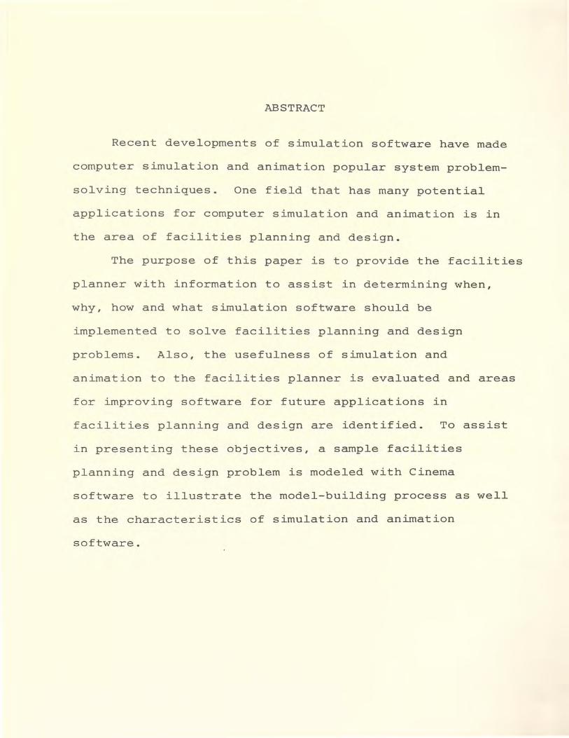
ABSTRACT

Recent developments of simulation software have made

computer simulation and animation popular system problem­

solving techniques . One field that has many potential

applications for computer simulation and animation is in

the area of facilities planning and design.

The purpose of this paper is to provide the facilities

planner with information to assist in determining when,

why, how and what simulation software should be

implemented to solve facilities planning and design

problems. Also, the usefulness of simulation and

animation to the facilities planner is evaluated and areas

for improving software for future applications in

facilities planning and design are identified. To assist

in presenting these objectives, a sample facilities

planning and design problem is modeled with Cinema

software to illustrate the model-building process as well

as the characteristics of simulation and animation

software.

TABLE OF CONTENTS

LIST OF TABLES .

LIST OF FIGURES

INTRODUCTION .

SIMULATION, ANIMATION AND FACILITIES .

Simulation and Animation Definitions Facilities Planning and Design

Applications

DESIGNING THE SIMULATION MODEL .

Problem Analysis Problem-Solving . Evaluation

SELECTING SIMULATION AND ANIMATION SOFTWARE

Simulation Software Features Animation Software Features . Comparison and Selection of Software

SIMAN SIMFACTORY . SIMPLE 1 . SLAM II Micro SAINT

Comparison and Selection of Software: Summary .

CASE STUDY: APPLICATION OF CINEMA .

Features of Cinema Evaluation of Cinema

SUMMARY AND CONCLUSIONS

APPENDIX: STUDY OF TOLL BOOTH FACILITY

BIBLIOGRAPHY .

iii

v

vi

1

3

3

6

13

13 19 22

26

26 30 30

31 34 36 38 39

40

43

44 48

53

58

77

LIST OF TABLES

1 Comparison of Five Simulation Software Packages .

2 Tolls and Toll Booth Usage by Vehicle Classification

3 Available Toll Booths in the East Toll Plaza

4 Configuration of Toll Booths Used at the East Toll Plaza from 2 p.m. to 7 p.m.

5 Tolls and Toll Booth Usage by Vehicle Classification

iv

• 32

. 61

. 63

. 63

64

LIST OF FIGURES

1 Simulation Model Categories and Their Relationship to the Real World . 5

2 A General Procedure for Designing A Simulation Model . 14

3 Layout of Toll Booth Stations • 68

v

INTRODUCTION

In the past few years, the term "simulation" has

received much notoriety as a system problem-solving

technique . Any current technical trade magazine,

especially those specializing in production, computers and

manufacturing, seems to be teeming with advertisements

proclaiming the virtues of simulation. One vendor of a

simulation software package claims "if it can be flow-

charted, it can be simulated" (Haider 1986). It is

estimated there are over 100 simulation software packages

currently available and competing for this "new-found"

market (Micro Analysis and Design Inc. 1987).

The latest trend in computer simulation has been the

increased use of computer graphics for animated displays of

the movement of entities through the simulated system.

Prior to animation, computer simulation results were

revealed primarily through printed output that summarized

the completed simulation. Animation allows the user to see

the simulation in process while providing data on the state

of the system being simulated as it occurs rather than in a

summary statement at the end of the simulation.

The new array of computer simulation software packages

has provided the opportunity to employ simulation in many

nontraditional applications. One of these applications is

1

2

the field of facilities planning and design. The intent

of this paper is to provide those involved in the

facilities planning process, who may not be experienced in

programming simulation languages, with the following

information:

* An awareness that simulation and animation, as a

result of advances in computer software, can

become a valuable tool for the facilities

planner.

* A procedure to guide the facilities planner in

determining when and why a simulation model should

be used to analyze a facilities problem and how

the model should be designed and evaluated.

* An evaluation of the features of simulation and

animation software that a facilities planner must

review when selecting an appropriate software

product for his model.

These points are illustrated with an example of a

facilities planning and design application using Cinema, a

popular simulation and animation product available on the

market today. This example is also used to formulate

conclusions on the value of simulation and animation

software to the facilities planner and to identify ideas

for improving the software for future applications in

facilities planning and design.

SIMULATION, ANIMATION AND FACILITIES

Vendors of simulation and animation software have

circulated much literature in the past few years that

advertises the uses of their products. However, it should

not be forgotten that these vendors are selling software

to make a profit. When should a facilities planner turn

to simulation and animation to study a facilities problem?

This section of the paper defines simulation and

animation, when simulation and animation should be

implemented and some of the possible applications in the

field of facilities planning and design.

Simulation and Animation Definitions

Simulate, in the broadest sense of the word, means

"to imitate." In a mangement sense, simulation is used to

imitate a real system in order to observe and learn from

the replica, or model. Models and the process of

simulation provide a convenient means whereby the

decision-maker may be provided with factual information

regarding the operations under his control without

disturbing the operations themselves. Thus, the

simulation process is essentially one of indirect

experimentation involving the alternative courses of

action before they are adopted.

3

4

Simulation is a type of model, specifically a

mathematical model. Models can be categorized according

to the degree of realism that they achieve in representing

a problem in the real world. The model categories and

their relationship to the real world can be seen in Figure

1. These model categories are:

1 .

2.

3.

Operational Exercise. This modeling approach

operates directly in the real environment in

which the decision is going to take place.

Gaming. A model is constructed that is an

abstract and simplified representation of the

real environment. However, all the people who

participate in the decision process in the

system being modeled also interact in the model

itself.

Simulation. Simulation models are similar to

gaming models except all human interaction is

removed from the modeling process. The models

provide the means to evaluate the performance of

a number of alternatives supplied externally to

the model by the decision-maker without allowing

for human interactions at intermediate stages of

the model computation.

4. Analytical Model. In this type of model, the

problem is represented in completely mathematical

terms which we use to maximize or minimize,

/

ti.M

AN

DE CIS~

..W.E

R I

S l

OF

Tt£

MOC

£LIN

G PR

OC

HU..a

AN

DECI

SWN

L4AK

ER

IS

EX

lER

NA

L 1

0

THE

MO

DELI

NG

PRO

CES

S

A.

r--

----

------.

ON

GJ

OPE

RAT

I EX

E RC

~MIN

G SI

MU

LATI

ON

AN

ALYT

ICAL

~ODEL

ISE

INCR

EASI

NG

DEG

REE

OF

ABST

RAC

TIO

N

AND

SPEE

D

/ IN

CREA

SING

DE

GRE

E OF

REALIS~

AND

COST

'

Fig

ure

1

. S

imu

lati

on

M

od

el C

ate

go

ries

and

T

heir

R

ela

tio

nsh

ip

to

the

Real

Wo

rld

(S

. B

rad

ley

, A

pp

lied

M

ath

em

ati

cal

Pro

gra

mm

ing

)

Ul

6

subject to a set of mathematical constraints that

portray the conditions under which decisions have

to be made (Bradley 1977).

Ideally, an analytical model would be the most

preferred choice when selecting a model because they

provide exact answers to the question of interest, and

they are the least expensive and easiest models to

develop. However, analytical models introduce the highest

degree of simplification in the model representation. It

is important when using such a model to ensure that the

resulting degree of realism is appropriate to characterize

the decision under study, and not the tool being used to

investigate the decision-making process, that should

determine the amount of information needed to handle the

decision effectively.

So, if an analytical model is the ideal choice for

modeling a system, when and why should a simulation model

ever be used? Unfortunately, most systems, including

projects in facilities planning and design, are too

complex to evaluate analytically, so they must be studied

by means of simulation.

Unlike analytical models, simulation models usually

do not produce an optimum answer to the decision under

study. These types of models are inductive and empirical in

nature: they are useful only to assess the performance of

alternatives identified previously by the decision-maker.

7

It then becomes the task of the user to heuristically find

a satisfying solution or a solution that the user is

willing to settle for to achieve the system objectives.

Most simulation models take the form of computer

programs, where logical arithmetic operations are

performed in a prearranged sequence. It is not necessary,

therefore, to define the problem exclusively in analytic

terms. This provides an added flexibility in model

formulation and permits a higher degree of realism to be

achieved.

Animation is not a model in itself but an enhancement

to a simulation model. Users of simulation software

packages that are accompanied with the animation option

can now graphically depict the system being simulated on a

graphics monitor. Dynamic symbols, representing entities

in the simulation model, move across a static

representation of the system on the graphics monitor to

show the flow of entities through the system. The

animation shows the present state of the system as it

occurs during simulation. Variables of the system, such

as elapsed time or queue sizes, can be displayed and

updated on the graphics monitor during simulation as well.

Facilities Planning and Design Applications

Escalating costs for construction and capital

equipment have prompted facilities managers to carefully

8

analyze the desirability of all new proposed facilities

before committing the funds for the projects. Some

performance measures that can be obtained through

simulation for evaluating the feasibility of new

buildings, building renovations or new equipment might be:

* throughput analysis of existing and proposed

facilities

* equipment/facility utilization

* time spent in queues

* time spent in the system

* return on investment

* space utilization

* payback periods

* distances traveled by equipment, personnel and

materials

To determine the desirability of a facility project,

a method for predicting the performance of the system must

be employed. For most facilities systems, such as

existing buildings, equipment configurations or national

distribution networks, experimentation within the system

would be disruptive to operations or just too expensive.

For proposed facilities, such as a new plant or building

expansion, it would be ridiculous to construct a facility

for experimentation purposes. Furthermore, most

facilities are too complex for analytic models.

9

Facilities modeling through computer simulation is easily

the most desirable alternative.

In the past, computer simulation was seldom used for

facilities planning and design. Simulation models were

originally constructed through general purpose computer

languages such as FORTRAN, and development of the models

required a lot of time, money and highly trained

personnel. Reduced computing costs, improvements in

simulation languages and simulation/animation software

packages that require no computer programming have enabled

computer simulation to become a valuable tool for

facilities planners and designers. Simulation can now

effectively save development time and financial resources,

thereby delivering reduced construction costs and more

efficient facilities.

Animation is a valuable tool for facilities

applications of computer simulation. Most importantly,

animation provides a means of communicating facilities

plans to those who have no knowledge of computer

simulation and programming. With the aid of a graphics

monitor and animation, viewers can watch the flow of

entities through a facility and observe the overall system

performance. Animated displays can draw people without

simulation programming experience into the model building

process. As they watch the model evolve over time on the

10

screen, ideas and suggestions seem to be more freely

generated and offered.

A recent development in computer simulation and

animation may prove to be valuable to those who prepare

facilities plans for the shop floor in manufacturing

facilities. There are several simulation software

packages now available for factory planning, such as

SIMFACTORY and MAP/I which require no programming. The

factory description and process flow are entered through a

menu-driven user interface. These packages make

simulation available for applications that were once

considered too small to justify a simulation programming

effort.

Some examples of facilities planning and design

projects that can be studied using computer simulation are

listed below:

* Proposals for new buildings. The building can be

viewed as a complete system for simulation

purposes. By simulating the network of operations

being performed within the building, the total

production of the building or system can be com­

pared by altering a parameter, such as the number

of receiving docks, to determine the effect on the

entire system. Simulation can be used for studying

such facilities as manufacturing plants, distribu-

11

tion centers, banks, fast food restaurants, gas

stations or hospitals.

* To determine the impact of new equipment installa-

tions. Different scenarios could be compared by

running a simulation for each piece of equipment

under consideration to determine its effect of the

total system. Equipment being installed could be

tried at different places within the facility to

determine the most effective location for the

equipment. Simulation could be used for setting up

Flexible Manufacturing Systems (FMS), group tech­

nology cells, assembly lines and Just-in Time (JIT)

systems.

* Material handling systems, such as automated

guided vehicles (AGV) or automated storage and

retrieval systems (ASRS), could be studied with

computer simulation to determine their required

size and optimal location. Other material

handling systems such as conveyors and overhead

material handling equipment could be simulated to

determine the minimum distances they will be

required to travel, thus reducing equipment and

installation costs.

* Site plans and highway and rail systems can be

planned and designed with the assistance of

computer simulation. Information provided from

12 .

simulation runs can aid in deciding how to route

the traffic flow and determining the size of the

required arteries.

* Construction and project planning techniques used

in facilities planning, such as PERT, can be

simulated to determine the critical path of the

project and the activity slack times.

Although these examples are just a few of the

potential applications of computer simulation in the field

of facilities planning and design, one can begin to see

the value of information provided by simulation output in

planning and designing efficient, cost effective

facilities. Animation, in turn, is valuable in selling a

plan or design to those who will eventually use or finance

the planned facility.

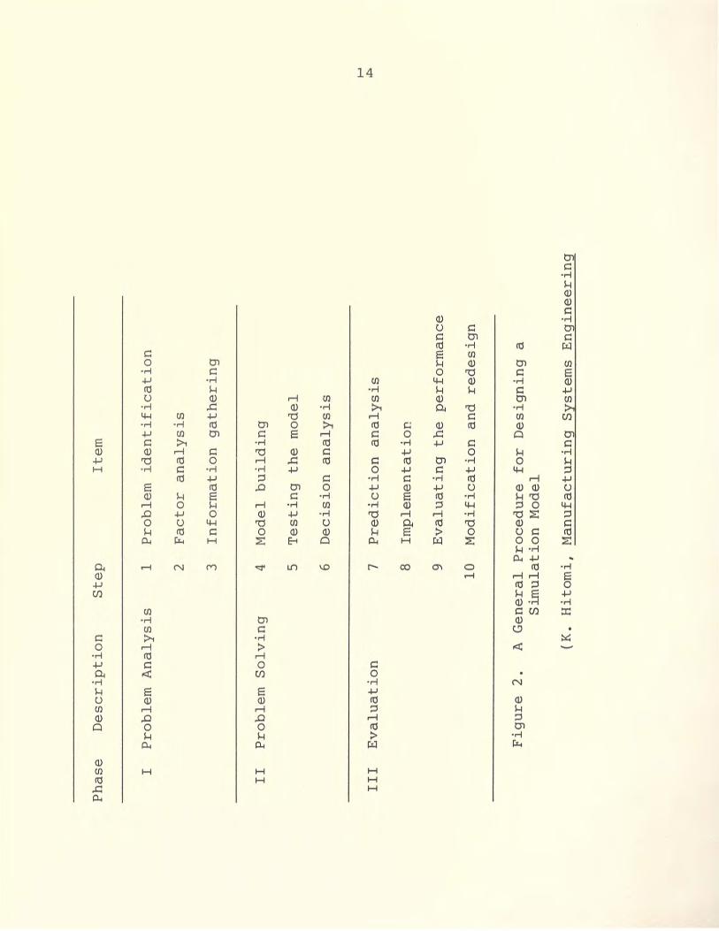
DESIGNING THE SIMULATION MODEL

One of the most challenging aspects of a modeler's

job is building an accurate model and convincing the end

users that it is an accurate representation of the system

being modeled. To ensure these objectives are met, a

well-conceived strategy for model design should be

prepared before the model is actually built. This

strategy should be a step-by-step procedure that will

enable the modeler to organize his modeling effort, set

intermediate goals and improve his modeling efficiency. A

general procedure for the design of a simulation model is

shown in Figure 2. This procedure describes the model

design as a three-phase process where each phase is

further described in terms of intermediate steps (Hitomi

1979). While this procedure is general and used for many

applications, it serves as an excellent guide for design-

ing simulation models.

procedure follows.

A detailed explanation of this

Problem Analysis

Problem analysis is the first phase of designing a

simulation model. The first step in this phase is to

identify the problem that has prompted the need for a

13 ·

Ph

ase

I

II

III

Descri

pti

on

S

tep

It

em

Pro

ble

m A

naly

sis

1 P

rob

lem

id

en

tifi

cati

on

2 F

acto

r an

aly

sis

3 In

form

ati

on

g

ath

eri

ng

Pro

ble

m S

olv

ing

4

Mo

del

b

uil

din

g

5 T

esti

ng

th

e

mo

del

6 D

ecis

ion

an

aly

sis

Ev

alu

ati

on

7

Pre

dic

tio

n an

aly

sis

8 Im

ple

men

tati

on

9 E

valu

ati

ng

th

e

perf

orm

an

ce

10

Mo

dif

icati

on

an

d re

desig

n

Fig

ure

2

. A

Gen

era

l P

roced

ure

fo

r D

esi

gn

ing

a

Sim

ula

tio

n

Mo

del

(K.

Hit

om

i,

Man

ufa

ctu

rin

g

Sy

stem

s E

ng

ineeri

ng

f--l ~

15

simulation problem and to determine the objectives that

one wishes to accomplish by selecting simulation as the

tool for solving the problem. The second step identifies

and lists the factors to be included in the design

problem. It is important in this step to distinguish the

controllable versus uncontrollable factors and the

qualitative versus quantitative ones. The controllable

and quantitative factors play fundamental roles in the

design of the model. The final step of this phase is to

collect the data and information that is necessary to

realistically model the system that is being studied.

During the first three steps, the modeler is

essentially gathering all the pertinent information that

will determine how the model is built. It is imperative

that the modeler takes every precaution to ensure that the

information he is using will result in a valid model. A

valid model is one which is sufficiently accurate to

achieve the objectives of the simulation and can be used

as a substitute for the real system. Equally important to

creating a valid model, the new model must be credible as

well. A credible model is one that is accepted by the

user as being valid and will be used as an aid in making

decisions (Carson 1986). If a model is not credible,

that model may actually never be used in a decision-making

process, even if it is valid.

16

Perhaps the most important factor in creating a valid

and credible model is that the modeler must work side-by­

side with the client and the people who work, or will

work, most closely with the system being modeled.

Together, they must define the overall objective of the

simulation, the issues to be investigated, the alternative

systems designs, the collection of input data and the

measures of performance.

While the modeler is collecting his input data for

the simulation model, he must constantly be aware of the

quality of these data if he is to construct a valid model.

A simulation is driven by its input and if the data are

poor, the model will not be valid.

There are several ways to get the data needed for

determining the inputs into the simulation model (Carson

1977). They are (in the order of their desirability):

* Time studies

* Historical records

* The best estimate of the vendor

* The best estimate of the client

* The best estimate of the modeler

Naturally, the most reliable input could be generated

by having someone perform time studies for the specific

needs of the model, but time and financial constraints

often will not allow this. Historical data can be

valuable but, preferably should be used only after

17.

conferring with the people who gathered the data.

Historical data collection by automated means may not be

as thorough as data collected through time study and

should be approached with caution as well. If the input

data required involves machines or material handling

equipment, the vendor may be able to supply processing

times, conveyance times or mean times to failure. These

times, as well as those estimated by the client or modeler

should be used only when the information cannot be

obtained by another means.

Regardless of the method used for accumulating the

input data, if the model is used repeatedly over time for

the same or new purposes, it should be remembered that the

system is always changing and the data are almost always

out of date or on the verge of being out of date. A

periodic evaluation may provide cheap insurance against

erroneous conclusions from an invalid model (Carson 1977).

Since a simulation model is a model of a real world

occurrence and real world occurrences are generally

random, the data input into the simulation model most

likely will be described as random variables. If a model

is random, it will contain one or more sources of input

random variables described by probability distributions.

A random number generator is used in simulation to

generate random samples from these input distributions as

the simulator advances through time. Examples of inputs

18

that might be described by random variables include

processing times, mean times to random failure or mean

time betwen arrivals of an entity.

When attempting to identify an appropriate

distribution for an input random variable, one of two ways

could be used to specify the distribution form: fitted or

empirical distributions (Kelton 1986). In using the

fitting approach, data would be explored through tools

such as histograms to determine if a distribution form is

suggested. Parameters for the chosen distribution, such

as mean and variance, could be derived from the data.

Goodness-of-fit tests could then be applied for determin­

ing if the distribution form selected was a good choice.

If the goodness-of-fit tests reveal a poor fit, the

process is repeated with another distribution form.

When using the empirical distribution approach, no

attempt is made to fit a standard theoretical distribution

form to the data. Instead, an empirical distribution is

defined directly from the data and the result is used as

the input distribution to the simulation. While the

empirical distribution approach is typically used when a

theoretical distribution does not describe the data, it

actually can be used in most any situation (Kelton 1986).

To summarize the first phase of designing the

simulation model, the objectives of modeling must be

clearly set and the parameters to be used in the model

19

must be closely scrutinized if a valid and credible model

is to be created. Most importantly, the model builder

needs to work closely with the user to ensure credibility.

An unused model is a waste of everyone's time.

Problem-Solving

The first step in the problem-solving phase is to

build the actual simulation model with the information

assembled from the problem analysis phase. The sinulation

model should have as little detail as necessary to address

the issues of interest but enough detail for it to remain

credible. As the model is being constructed, a periodic

walk-through of the model's flow chart should be conducted

with the users to maintain this credibility. If the user

has a similar existing system to the one being modeled,

the modeler should simulate this system as well. The

output of this simulation can be used for comparison with

the output of the new model as an additional check for

validity.

When building the model, it is suggested to get a

simple model up and running as quickly as possible, and

then later embellish it. This is a good way to maintain

the client's interest and involvement. As the model

continues to grow with more detail, use of structured

techniques such as modularity and top-down design are

recommended. These will ease the debugging process.

20

The model-building step will vary greatly in duration

depending on the complexity of the model and the software

used for the simulation model. General purpose languages

such as FORTRAN may require the most time to create a

model but, on the positive side, they are very versatile.

Simulation languages such as SIMSCRIPT or SIMAN greatly

reduce the programming time for most simulation

applications and, depending on the language, can be

accompanied by FORTRAN sub-programs if necessary. New

special purpose simulators, such as SIMFACTORY, require no

programming knowledge from the model builder, just a

knowledge of the parameters and the process being

simulated. Models can be built quickly but applications

are limited. Most model builders may not have a library

of simulation software packages available to them so the

models will be built with whatever software is most

accessible.

The next step in the problem-solving phase of

designing simulation models is the test of the model for

effectiveness. This is a check to determine if the model

constructed will achieve the results it was designed for.

One method is to run a trial simulation run and compare

the results with a similar existing operation. This may

help determine whether the results of the model are within

reason. If the language being used prints a comprehensive

set of output data, this information can also be h_elpful

21

in identifying errors in the model. For instanc€, a

utilization of zero may indicate that no product is

getting to a particular machine. A utilization of 100%

may indicate an erroneous capacity, an inaccurate service

time or an error in product routing (Carson 1986).

The use of a trace can also be employed as a

technique for verifying a simulation model. A trace

consists of a detailed output that represents the step­

by-step progress of the simulation model over time. A

trace can be of special value for detecting the cause of

subtle errors and verifying that the model can handle

unplanned circumstances, such as running out of materials

or having a piece of equipment go down. Almost all

simulation languages have a tracing capability and some of

these languages also have an interactive debugger that can

be used with the trace.

Graphical animation of the simulation can be also

used as a means of verifying the model. Animation is

essentially a visual representation of a trace. The model

builder can view the flow of entities through the system

to see if the simulation is performing as was intended in

the model.

The final step in the problem-solving phase is

decision analysis where alternative designs to the

original model are experimented with in an effort to find

a level of model performance that the user is willing to

22

settle for. Since simulation is not an optimization

technique, a near-optimal solution is usually appreciated

by the user under these circumstances.

Evaluation

The third phase of designing a simulation model

involves the evaluation of the simulation model that was

analyzed and built in the two previous phases. The steps

in this phase are prediction analysis, implementation,

evaluating the performance, and modification and redesign

of the model.

During the prediction analysis step, the "near­

optimal" solution is evaluated as a real world solution.

If the result of this analysis is not satisfactory, the

modeler returns to the model-building step for further

rework. If the result of the analysis is satisfactory, we

can proceed to the implementation step, where the system

being simulated is installed and the procedure is executed

in the real world.

In the next step, the actual results of the

simulation are measured and evaluated by the following

criteria:

* Reliability--Accuracy of performing and enduring

the specified functions and goals of the system

when installed

23.

* Response--Ability of the system to adapt to the

change of the environment or the disturbance

* Stability--Abilty of the system to maintain a

stable state even with substantial changes in the

environment

* Adaptability--Ability of the system to maintain

optimality

* Economical eff iciency--Assurance of implementing

the system economically

When evaluating the simulation model, it should be

remembered that many models require a "warm-up" period

before the system reaches "steady-state." When a

simulation begins, the system is usually in an empty or

idle state. In a real-life situation, this is not

realistic, as there is often already work-in-progress in

the real-life system that the simulation is attempting to

model. Therefore, simulations are often run for a certain

amount of time, called a warm-up period, before the output

data are actually used to estimate the desired measures of

performance.

One of the most common errors made when evaluating a

simulation model is making only one run of a stochastic

simulation. Since the inputs into the simulation model

are random variables, one simulation run will provide only

one observation from a probability distribution. Using the

results of one simulation run as the accepted solution

24

would be like trying to estimate the mean of a population

in classical statistics with exactly one data point.

Several simulation runs, depending on the level of

confidence desired, should be used before the simulation

is considered complete.

A complete statistical analysis should be performed

before summarizing the results of the simulation.

Ignoring the statistical aspects of simulation can result

in inaccurate, or even misleading results and conclusions.

The statistical aspects are beyond the scope of this paper

but there is much literature on this subject that could be

consulted for clarification. (See literature by Law and

Welch noted in the Bibliography for further information.)

The final step in the design of a simulation model is

the modification or redesign of the model. This is done

when the deviation between the actual performance and the

standard established in the planning stage is in excess of

limits determined by the user or client.

In summary, the design of a simulation model can be a

complex process that can require a preplanned procedure to

maintain organization and control once the project is

undertaken. Care must be taken at each step in this

procedure to ensure that a valid model is being

constructed. The decision to simulate can be a major one

and so management must be willing to make the commitment

to support the effort. The design of the model may

25

require the efforts of programmers, industrial engineers,

manufacturing and production control personnel,

supervisors, foremen and plant management. It is

imperative that they provide the modeler with information

regarding the real system operation because it is they who

will ultimately pass judgement on the validity of the model

and pass that judgement up the line to top management.

SELECTING SIMULATION AND ANIMATION SOFTWARE

Before purchasing simulation software, an inventory

of one's software needs and expectations should be taken.

There is such a wide variety of simulation software now

available that if one can clearly define his simulation

objectives, he could probably find the software that is

custom-made to fill his requirements. The remainder of

this section reviews the features of simulation and

animation software and compares five selected software

packages available on the market today.

Simulation Software Features

All simulation software can be classified according

to its traits in each of three different areas. These

areas are the type of system being modeled, the

application the software is needed for and the modeling

orientation employed by the simulation software.

There are two types of systems that are generally

recognized in simulation modeling--continuous and

discrete. A software package might have the capability to

perform continuous or discrete simulations or both. In a

continuous model, the parameters, or state variables,

change continually over time. In a discrete model, the

26

27

state variables change only at discrete points in time

called events.

The second area of classification for simulation

software describes the application of the software.

Simulation software can be classified as either special

purpose or general purpose. A special purpose simulation

software package is one that has been designed

specifically for simulating a specific environment. The

use of these packages may result in an additional

reduction in programming time since their modeling

constructs are oriented to a specific environment. The

most common special purpose software is for modeling

manufacturing or material-handling systems. These special

purpose simulation software products are generally called

"simulators." General purpose simulation software

products, called "simulation languages," allow one to

model almost any system and to perform almost any type of

analysis but more expertise and effort are required. Many

simulation languages allow for subroutines written in

another language such as FORTRAN to further improve the

language's versatility.

The third area of classification describes the model

orientation employed by the software. The two most common

orientation descriptions are process and event

orientation. Process orientation allows the modeler to

depict the system being modeled through a block diagram or

2a

flow --chart. In event scheduling, the system being modeled

is reviewed as consisting of a number of possible events

at which state changes take place. The modeler must

define events and develop and program the logic associated

with each.

When selecting a software package to purchase or

lease, the three areas of simulation software

classification just described must be reviewed to

determine the type of software needed. There are other

features in simulation software packages that should be

reviewed during the selection process.

described as follows (Haider 1986):

These features are

1. Input flexibility--The software design should

allow the flexibility for developing models in a

batch model or in an interactive environment. A

nice feature, with process orientation, is the

ability to generate a network flow chart from

the input statements or vice versa.

2. Syntax--The syntax used in the simulation

software package should be user-friendly,

consistent and nonambiguous. This will aid in

faster model development.

3. Structured modularity--Simulation software

should allow modular development of a model for

ease in construction and debugging.

29

4 . Material handling module--This is a time-saving

feature for those who model within a

manufacturing environment because material­

handling systems are difficult to model.

5 . Statistics generation and data analysis--A

comprehensive means of collecting and displaying

data. Important in analyzing and communicating

the results of a simulation.

6 . Interactive model debugging--This feature can

significantly reduce the time it takes to

construct a model.

7. Micro/mainframe compatibility--If a simulation

software package offers micro/mainframe

compatibility, it becomes available to a wider

variety of users who may already have the

necessary hardware. If a user has both a

mainframe and a microcomputer, he can develop

the models using a microcomputer, which is

generally more accessible, interactive and has

no associated cost for computer time, and run

the simulation using the mainframe, which is

significantly faster and more powerful.

8. Documentation and support--A good product with

poor documentation and little support will have

few satisfied users.

30

Animation Software Features

Many simulation software packages offer animation as

an enhancement to the simulation. The major constraint in

selecting an animation package is that the animation is

tied to a specific simulation language. Animation

packages are not interchangeable among different

simulation languages. The best simulation language may

not be accompanied by the most desirable animation package

or vice versa.

Some factors to consider when reviewing animation

software features are two- or three-dimensional graphics,

graphic display characteristics, ease of constructing

graphics screens, the ability for user interactions during

simulation, the hardware required and, of course, cost.

Comparison and Selection of Software

When selecting simulation software, one is selecting

a package that contains a simulation language, the brand

and type of hardware and possibly an animation option.

The type of simulation problems that can be solved in the

future is also being selected at the same time. In order

to make an intelligent choice of software, it would be

best to investigate the classifications of problems that

are expected to be solved with simulation and the users who

will be creating and using the models. By identifying

this class of problems, (i.e., discrete simulation

31

problems concerning manufacturing process plans and

requiring two-dimensional, interactive graphics), and the

users (i.e., manufacturing engineers with no programming

experience and little spare time), a comparison of

different simulation software packages can be made to

these specifications.

Table 1 displays a comparison of the characteristics

of five different simulation software packages on the

market today. They are: SIMAN, SIMFACTORY, SIMPLE I,

SLAM II and Micro SAINT. A brief description of each of

these software packages is included on the following

pages.

SIMAN

SIMAN is a combined discrete event, network and

continuous simulation language initially developed in 1983

for implementation on mainframe and personal computers.

The structure of SIMAN is based on concepts in which a

distinction is made between the system model and the

experimental frame. The system model defines the static

and dynamic characteristics of the system being modeled.

In comparison, the experimental frame defines the

experimental conditions under which the system is to be

studied. By separating the model structure into two

distinct elements, various simulation experiments can be

TA

BL

E

1

CO

MPA

RIS

ON

O

F F

IVE

SI

MU

LA

TIO

N

SOFT

WA

RE

PAC

KA

GE

S

Mic

ro-

SI M

AN

SIM

FAC

TOR

Y

SIM

PLE

1

SLA

M

II

SAIN

T

--

Dis

cre

te/

Co

nti

nu

ou

s B

oth

D

iscre

te

Bo

th

Bo

th

Dis

cre

te

Gen

era

l P

urp

ose

/ S

pecia

l P

urp

ose

G

en

era

l S

pecia

l G

en

era

l G

en

era

l G

en

era

l

Ev

ent

Ori

en

tati

on

Y

es

No

Yes

Y

es

No

Pro

cess

O

rien

tati

on

N

etw

ork

/Use

r W

ritt

en

N

etw

ork

N

etw

ork

N

etw

ork

N

etw

ork

N

etw

ork

Inte

racti

ve

Deb

ug

Yes

N

o Y

es

Yes

N

o w

N

M

ate

rial

Han

dli

ng

F

eatu

re

Yes

Y

es

No

Yes

N

o

Mai

nfr

ame/

PC

B

oth

PC

PC

B

oth

PC

An

imat

ion

C

inem

a Y

es

Yes

T

ESS

N

o

Pre

pro

cess

or

BLO

CK

S N

/A

No

Yes

Inte

racti

ve

Dis

pla

y

Gen

era

tio

n

Yes

Y

es

No

Yes

Mu

ltip

le

Dis

p.

, M

ult

. M

ult

. Z

oom

, P

an

Yes

D

isp

. D

isp

. Y

es

Use

r C

reate

d

Men

us

& H

ELP

Scre

en

s Y

es

No

Yes

Y

es

33

generated simply by altering values specified in the

experimental frame.

With SIMAN, component models based on three distinct

modeling orientations can be combined in a single system

model. For discrete change systems either a process or

event orientation is used for modeling. The process

orientation is used to model discrete change systems and

uses a block diagram to depict the flow of entities

through the system. This can be achieved with BLOCKS, an

interactive, menu-driven, self-explanatory graphic model­

builder for creating, editing and viewing SIMAN model

files. In the event orientation a user is required to

supply FORTRAN subroutines to describe the event logic.

These user-written events can be embedded within a block

diagram to allow for options not covered by a SIMAN block.

The continuous change systems are modeled by a set of

algebraic or differential equations.

SIMAN uses five processors to load and execute a

simulation (Pence 1984). They are:

1. MODEL--Builds a block diagram model.

2. EXPMT--Specifies parameter values of the

experimental frame.

3. LINKER--Links the model and the experiment to

create a program file.

4. SIMAN--Executes the simulation runs and writes

any user-specified responses to an output file.

34 ·

5. OUTPUT--Performs data analysis functions on the

data stored in the output file using barcharts,

correlograrns, histograms, confidence intervals,

plots or tables.

SIMAN has the capability to extensively model

material-handling systems. However, SIMAN is a general

purpose simulation package and considered to be very

versatile.

with SIMAN.

Animation software called Cinema is available

One of the most significant features of SIMAN is that

its models are fully transportable between a microcomputer

and a mainframe computer. Unlike many other simulation

languages, the same version can be used for either the

microcomputer or mainframe.

SIMFACTORY

SIMFACTORY has been designed as a tool for producing

simulation models and animations specifically for studying

the manufacturing of discrete part products; it was never

intended to be a general purpose simulation language.

There is no simulation programming involved when using

SIMFACTORY. Instead, the modeler will enter production

parameters and factory layout information using

SIMFACTORY's menu-driven user interface and SIMFACTORY

will create the simulation model using a general

35

manufacturing model developed using the SIMSCRIPT II.5

simulation language.

The SIMFACTORY user interface consists of 12

different menus. The user creates the model by selecting

corrunands from these menus via cursors and a minimal amount

of keyed input. After the complete data set has been

defined for the factory, the user returns to the main

menu, selects its run command and SIMFACTORY will begin to

read the data set, initialize the data and simulate the

factory. During the initialization phase, SIMFACTORY

will check the data for consistency and identify any

errors. If no errors are detected, SIMFACTORY will

proceed to the simulation. SIMFACTORY automatically

produces an animated picture of the factory at work. [It

is highly recorrunended that validation runs be made prior

to checking out the production runs.

especially helpful for this purpose.

The animation is

However, the

animation does slow down the execution by a significant

factor. Therefore, it is suggested the animation be

suppressed when making production runs.]

SIMFACTORY features include a trace function, the

ability to simulate material-handling equipment and a

statistical surrunary report. Summary reports can be

produced for the following parameters:

* process station utilization

* transporter utilization

* resource utilization

* queue levels

* throughput

36

* raw material consumption

The hardware required for installing SIMFACTORY

includes an IBM PC/AT and an IBM Enhanced Graphics Display

(or their equivalents).

SIMPLE I

SIMPLE 1 is a modeling environment for interactive

simulation using the IBM PC, AT or other compatibles.

Models are written in SIMPLE 1, a new discrete and

continuous network simulation language. The language was

designed and ideally suited for analysis of manufacturing

systems. However, SIMPLE 1 is a general purpose language

that can be used for many other applications besides

manufacturing analysis. The SIMPLE 1 software package

also includes character animation of the simulation

results.

SIMPLE 1 utilizes a network diagramming approach to

model construction. Models are built conceptually by

interactive construction of network diagrams similar to

activity or flowcharts; no programming is required. The

user is provided modeling support for file building,

editing, compilation and execution of simulation models.

Access to the utilities which aid in performing these

37

tasks is at the MAIN ENVIRONMENT level of the software.

The network diagrams constructed by the modeler are

converted to SIMPLE 1 simulation language code when the

model is compiled. SIMPLE 1 statements are composed of

key words, mathematical and logic operators, user-defined

variables and block labels. Since the language is

statement-oriented versus line-oriented, statements can

span multiple lines and short statements can be grouped

onto one line.

Models using SIMPLE 1 are built in five segments:

1. DECLARE--Defines global variables, entities,

screens and files.

2. PRERUN--Initializes program variables and run

parameters.

3. DISCRETE--Contains the description of the model

structure using a discrete network.

4. CONTINUOUS--Contains the description of the model

structure using a continuous network.

5. POSTRUN--Analyzes run results and performs run

control tasks.

Histograms, plotting and other analysis functions can

be performed using library models and printed by SIMPLE 1.

SIMPLE 1 also has an editor debugging feature. When the

compiler detects an error, the editor is automatically

called. The editor will be initialized with the cursor

38

posit ion at the location in the file where the error was

de t ected .

SLAM II

SLAM II is a FORTRAN-based simulation language that

provides network, discrete event or continuous modeling

approaches . Any of these approaches can be used

singularly or in combination in a simulation model. A

SLAM II simulation model normally begins with a network,

or flow diagram , which graphically portrays the flow of

entities through the system (Lilegdon, 1985). No pro­

gramming skill is required, just the ability to reproduce

the network of nodes and routings that comprise the system

to be modeled. SLAM II will prompt the user for this

information. There are 20 node types available in SLAM II

for such functions as entering and exiting the system,

seizing or freeing a resource, changing variable values,

collecting statistics and starting or stopping entity flow

based on system conditionsn The routings that connect the

nodes may be deterministic, probabilistic or based on

system variables.

When a model calls for more complex discrete event

processing than allowed by the network, SLAM II provides

easy access to FORTRAN subroutines. FORTRAN also is

availble when coding any equations that define continuous

variables. SLAM II provides the ability to combine these

39

user-written events and continuous variables with network

constructs as required.

To simulate a model using SLAM II, three separate

processors are required: INPUT, EXECUTION and OUTPUT.

The INPUT module is used to interpret the SLAM II control

and network diagrams into statements. These statements

are stored in a file and can be modified by any editor.

As the input processor executes, it checks for errors in

the coding. These errors must be corrected before

analysis can continue.

The EXECUTION processor uses the file created by the

INPUT processor to simulate the interpreted model. When

simulation is completed, the accumulated statistics and

system status are written to a disk file. The OUTPUT

processor can then be used to produce tabular reports from

this disk file.

SLAM II also features a system trace for model

verification and debugging, and an animation option called

TESS. SLAM II can be installed on a variety of mainframe

and minicomputer systems using standard FORTRAN. It can

also be fully implemented on the IBM PC and other

compatible minicomputers.

Micro SAINT

Micro SAINT is a tool for constructing simulation

models on an IBM PC (or equivalent) by responding to

40

interactive menus rather than prcgrarnming in a simulation

language . The procedure for modeling with Micro SAINT is

to describe the process or system to be simulated in terms

of a flowchart or network and select the task network

option from the master menu. The menu-driven user

interface will prompt the modeler for information

concerning each activity in the network. Micro SAINT

provides on-line help if it is needed by the modeler.

Execution of the simulation models is interactive.

The simulation may be paused during a run so that the

values of any of the variables can be changed during

execution. Micro SAINT provides no animation graphics

although it can graphically depict a diagram of the input

task network. The analysis option provides bar charts,

line graphs, scatter plots, step charts and time lines as

well as a few simple statistical calculations. Micro

SAINT can simulate models that have up to 400 tasks and

100 variables.

Comparison and Selection of Software: Summary

As the five simulation software packages were

reviewed, it became apparent that many offered some of the

same features. Some of the trends in simulation software

are:

* Implementation on microcomputers

* Manufacturing oriented preprocessors

41

* Lower priced systems

* Interactive operation in both the simulation/

animation operation and in display and model

building

* The ability to generate a network or flow · chart

from the input simulation program and vice versa

when in process orientation

All five software packages could be used for

facilities applications of some sort. Micro SAINT clearly

had the most limited types and numbers of applications:

the creation of models from user-interface menus limits

its versatility and it had no available animation package.

However, it was probably the easiest to use. On the other

hand , SIMAN and SLAM II could simulate nearly any model,

providing versatile languages, the addition of subprograms

and the ability to run on a mainframe if the model was too

complex or large for a minicomputer. Both have plenty of

less important, yet nice perks that help these languages

stand out from the others. Perhaps the only factor that

separates them would be one's preference or comfort in

using of the languages.

SIMFACTORY was the only manufacturing simulator

reviewed. It would be helpful in planning facilities

layouts in the factory or developing material-handling

systems but has limited application beyond that. It is

valuable in solving smaller simulation problems that one

42

could not normally justify a simulation model for before

manufacturing simulators were developed. Model

development is very fast and does not require a lot of

skill.

As always, one gets what one pays for.

CASE STUDY: APPLICATION OF CINEMA

An example of a facilities planning and design

application utilizing simulation and animation software

has been developed to illustrate the procedure for design­

ing a simulation model as presented in the paper. This

simulation model also provides the opportunity to use and

review a software product called Cinema. The example

application, a model of the east toll plaza on Orlando's

East-West Expressway, appears in the Appendix. The

Appendix includes a discussions of the situation being

modeled, how the model is constructed in the simulation

language, the results of the simulation and further

applications of this model.

The toll plaza was selected as an example because it

is a nontraditional facilities planning and design problem

that illustrates that a wide variety of applications can

be modeled with simulation and animation software, rather

than the traditional machine shop demonstrations that the

vendors include with the software. The toll plaza can

also be clearly understood when animated, as it is not too

visually complicated. Furthermore, anyone who has

travelled the highways of Central Florida can understand

this problem.

43

44

In this section of the paper, the features of CiQema

are discussed as well as an evaluation of the performance

of Cinema, based on the outcome of the toll plaza

simulation presented in the Appendix.

Features of Cinema

The software package used in this example was Cinema

version 2.1, which was available in the Industrial

Engineering Computer Lab at the University of Central

Florida. This is not the most recent version of Cinema

software available on the market. Cinema is a simulation

and animation software package that joins a SIMAN

simulation model with an animated layout of the model.

Both Cinema and SIMAN were developed by the Systems

Modeling Corporation of State College, Pennsylvania.

Cinema requires the following hardware for operation:

* IBM PC/AT or compat1ble with 640K bytes of memory

* 80287 Math Co-processor

* High resolution graphics board

* 19" color monitor

* Mouse

The animation construction is a two-step process.

The first step is to build the simulation model using the

SIMAN language. The second step is to build an animation

layout of the model described in the first step using

45

Cinema. The SIMAN model and the animation layout are

brought together to generate the real-time simulation.

The basic construct of Cinema is the animation

layout. This layout is a combination of objects that

comprise the system being simulated. There are two types

of objects in an animated layout in Cinema: static and

dynamic objects.

The static objects form the background of the layout

and represent the objects that do not change during

simulation. The dynamic objects represent the objects

that change during a layout. These objects are

superimposed over the static layout. Examples of dynamic

objects would be workers, workpieces, material-handling

equipment, machines or robots.

When preparing the animation layout using Cinema, all

user interfacing is performed with a mouse, which is a

hand-held pointing device that controls the motion of the

cursor on the screen. The commands for Cinema are pull-

down menus that appear on the screen. To activate a

command in Cinema, simply move the mouse across the desk

top until the cursor rests on the desired command. The

command is activated by selecting one of the two buttons

on the mouse.

The static background is drawn by selecting commands

from a drawing function menu. These commands might

include line, box, bar, circle or arc. These elements can

46

be placed using different colors, styles and line width.

Text can also be placed in the layout.

The dynamic objects in the layout are tied to

specific modeling constructs within the accompanying SIMAN

program. As the state of the simulation changes in the

SIMAN program, the dynamic objects are automatically

updated in the Cinema layout. The following listing

describes the main dynamic objects in a Cinema layout.

These objects can be created using the mouse and the pull­

down menu.

* Entities--This is the most common dynamic object

in Cinema and usually represents a job, work-

piece or customer. It is usually shown on the

screen as a drawing of the object it is

representing. The entity moves about the

screen in the animated layout as its counterpart

moves from station to station with the SIMAN

model.

* Queues--Entities residing in queues in the SIMAN

model can be shown in a queue on the animated

layout.

object.

The queue is another dynamic or changing

* Resources--A resource is a dynamic object that has

a fixed location in the layout. The resource symbol

shown in the layout is tied to a resource in the

experimental frame of the SIMAN model and is

47

shown in one of four states:

or pre-empted.

idle, busy, inactive

* Transfers--This dynamic object defines the paths

which entities travel in the layout.

* Storages--A storage is used to define a set of

places where entities are located when they do not

appear on the layout.

Another piece of information that can be displayed on

the animated layout is the variables that describe the

state of the system during simulation. Examples of these

variables are current simulated time, number of entities

in a queue or number of workpieces completed. Display

variables can be identified on the layout using any of the

following display features:

* Represent the variable value in a digital display.

* Graphical displays using the level feature: a box

with a bar inside that moves up and down to

represent the level, a circle that works similar

to the box and a dial that works like a gauge.

* A global symbol representing an entity that

changes in appearance when the status of the

entity changes.

* The color of an object on the animation layout can

change as a variable changes in value.

48

The newest version of Cinema, version 3.5, primarily

offers an improvement in the graphics for the static

layout . A dimensionally correct layout can be created

using any CAD program that outputs DXF files and read into

the Cinema static layout. However, the dynamic

compon ents still must be created using the Cinema

graphics , which lacks the capabilities to create

dimensionally correct or scaled graphics. This is still

an improvement over version 2.1, where both the static and

dynamic components must be created with Cinema graphics.

Cinema version 3.5 costs $14,000 for the EGA (Enhanced

Graphics Adapter) version and $28,000 (including

additional hardware) for the HGA or high-resolution

graphics version.

In summary, dynamic objects, static objects and

display variables can provide the graphical animation of a

model when tied into a SIMAN program. More information on

the details of constructing a Cinema animation can be

obtained from the Cinema System Guide supplied by Systems

Modeling Corporation or through Cinema's "Help" menus.

Evaluation of Cinema

Cinema can be evaluated in terms of its simulation

and its animation performance. In my opinion, the

simulation performed well while the graphics offers room

for improvement. This can be expected since the

49

simulation language has been in development much longer

than the animation. Perhaps the greatest improvement in

the simulation is the ability to perform simulation on a

personal computer instead of a main frame computer. The

convenience of the personal computer does have one major

setback: a simulation run can take much longer. This was

evident in the toll plaza example, which took over 30

minutes to complete the simulation.

There are several features of SIMAN simulation

software that deserve special mention. The TRACE and

interactive debugger features are valuable tools for

debugging and reviewing the performance of a simulation

program. The TRACE command provides the programmer with

the sequence in which the commands in the simulation

program are executed and the values of different

parameters at each command. The interactive debugger

allows the programmer to interrupt a simulation program at

any point during execution and obtain information on any

of the parameters or system variables.

The material-handling features of SIMAN, though not

used in the toll plaza example, are valuable features that

have simplified programming when material-handling devices

such as conveyors, industrial trucks or cranes are

required in the model. This feature also provides

50

performance parameters for any material-handling devices

used in the model.

SIMAN offers a thorough standard summary report for

any counters, tally variables or discrete change variables

requested. However, these reports are very inflexible and

provide only statistics that are available in the standard

report. It would be nice to give the programmer the

option of requesting the standard summary report forms or

specific statistics for specific parameters and system

variables.

The best features of the animation in Cinema are

variety of colors available and the ease in which the

display can be colored, the ability to display and update

variables on the graphics monitor during simulation, the

easy-to-follow pull-down menus that are used to construct

the static and dynamic components and a decent supporting

documentation for the animation. The most annoying

problem faced when working with the graphics was that the

display would frequently freeze during the construction of

a layout, causing the system to be rebooted. All input

since the last time the file was saved is lost. The user

must frequently save his graphics files during

construction so that hours of work would not be wasted.

The biggest disappointment with the graphics in

Cinema is that the graphics are for "artwork" and have

little value to the engineer other than for presentation

51

purposes. The graphics commands available in Cinema are

very crude and cannot be used for drawing with accuracy

or for much detail. The command for exploding the screen

to work details is also primitive and performs slowly.

The layout of the static background, due to the inability

to draw to dimensions with Cinema, will never be anything

more than a simplified schematic. The facilities planner

is unable to use Cinema animation to determine space

requirements for work-in-progress storage, equipment or

material-handling equipment.

Cinema version 3.5 provides a partial solution to

this problem. Layouts can be performend on a CAD system

and read into Cinema as the static background. However,

the dynamic components of the layout must still be

constructed with Cinema's crude drawing commands and,

therefore, cannot be constructed to scale. The software

also restricts the size that dynamic components such as

entities and resources can be constructed. This often

means that these dynamic components will not even look

proportional to the static background.

A further weakness of Cinema is the inability of

objects on the screen to recognize other objects. Objects

could collide (or run over any humans in the layout) and

the simulation would continue as if nothing happened.

This weakness prevents the simulation model from being a

realistic model of the situation being studied.

52

In summary, Cinema provides a. good simulation product

and the animation can be a good presentation tool for a

simplified schematic of the simulation. However, further

advances must be made to provide a more sophisticated

graphics package if the product is to become a space

planning tool for the facilities planner.

SUMMARY AND CONCLUSIONS

Simulation is a method of observing and learning

about a real system by studying a model of that system. A

simulation model should be used when a system is too

complex to study through an analytical model and it is

impractical (or impossible) to study the system in its

real environment. Since these conditions are often true

when studying a physical facility, simulation could become

an 1mportant tool in the field of facilities planning and

design.

Designing a simulation model for a complex system can

be a complicated process. A ten-step procedure for

designing a simulation model was described. This

procedure could be a valuable tool in planning and

controlling the design process. Throughout the design

process, the overall objective is to construct a model

that is both valid and credible. Maintaining close

contact with those familiar with the system being

simulated and carefully analyzing the quality of the input

data are two ways of ensuring a valid model is built.

Simulation models most commonly take the form of

computer programs and many advances in simulation software

in recent years have made computer simulation a more

53

54

popular problem-solving techniqu6. Two recent trends in

simulation have been software that is adaptable for use on

a person al computer and the graphical animation of simulation

models . Selection of the right software requires a

thorough understanding of one's own simulation objectives

and a knowledge of simulation and animation features

available to the prospective buyer.

There is no single ideal simulation software package

that is recommended for facilities planning and design

applications; simulation needs for these applications will

vary . An architectural and engineering firm that is

designing an airport may require a versatile simulation

language with a high-powered mainframe computer for

complex simulation, and animation for displaying the

simulation results to the elected public officials and

taxpayers that do not understand simulation. A shop floor

industrial engineer may be perfectly content with a

manufacturing simulator and no animation to use for

calculating the size of work-in-progress stockrooms

required when production is increased. To identify an

"ultimate" software package for facilities applications

was not the objective of this report, but rather to create

an awareness that simulation is a valuable, and, with the

many new software advances, also a feasible tool for

solving facilities problems.

55

While simulation has been a proven tool for modeling

complex systems for years, it had a limited number of users

because of the expensive computer hardware required and the

difficult-to-use languages that required skilled computer

programmers. Simulation software can now be used on

personal computers and the languages have made modeling

much easier. The result is that simulation has evolved

into a valuable tool with many applications that can be

used by many people, such as facilities planners.

Animation, however, is a new product that has yet to evolve

into a versatile tool. Several advances must occur before

animation software becomes a necessity for the facilities

planner.

At the present time, animation can be described as a

presentation tool rather than an analytic tool. Animation,

with its variety of colors and ability to display changes

in system variables and other parameters, is most valuable

for viewing a schematic that displays the activities that

occur during a simulation run. Animation is helpful when

presenting a simulation model to nontechnical personnel who

do not have the ability or the desire to understand the

simulation language program.

Animation will never be more than a presentation tool

until it has the capability of constructing graphics with

respect to dimensions. Animated objects move about the

screen without the ability to recognize other objects,

56

which hinders the simulation from performing like the rea'l

world system it is attempting to model. The lack of

dimensional accuracy prevents the modeler from determining

any actual distances traveled, the space required for

queues or the effect of rearranging the resources. Even

advances such as Cinema's version 3.5, which allows a CAD

layout to be used as the static background in the

animation, only improve the presentation qualities of

animation. The animation cannot become an analytic tool

until both the static and dynamic components can be

constructed with dimensional accuracy and the user is able

to interact with the graphics during simulation.

Another pitfall of animation software in its present

state is that animation graphics are not compatible with

different simulation languages. If one selects a

simulation software product, he is forced to use its

accompanying animation package. The best simulation

software for an application may not be available with the

best animation software for that application.

An ideal advancement from a facilities planner's

perspective would be the marriage of a full-scale

interactive graphics system, such as those offered by

Intergraph or Computer Vision, with any simulation

language. This would allow the facilities planner to

simulate within the actual facility plan as it would occur

if the facility were built. It would provide the ability

57

to move attributed entities through the layout in three

dimensions for analyzing object maneuverability and spatial

requirements. Such a system would eliminate the need for

recreating the layout in the animation graphics and

duplicating hardware since existing plans created with CAD

can be used. Interactive graphics would enable the user to

stop the simulation during a run to obtain descriptive

information from the layout. The animation graphics would

now have all the capabilities of CAD graphics such as zoom,

larger file capacity, report generation, cell creation

capability, improved drafting capability, dimensional

accuracy and the ability to overlay other drawings.

Despite some of the shortcomings of animation,

simulation and animation are still valuable tools in

facilities planning and design applications. While

animation has improved the facilities planner's ability to

present his simulation models, advances in the software

market must be made before it can be used as an analytical

tool.

APPENDIX

STUDY OF TOLL BOOTH FACILITY

PROBLEM STATEMENT

As one of the fastest growing counties in the

country, Orange County (Florida) is faced with the

challenge of providing an adequate transportation system

for its growing numbers of residents and visitors. This

transportation system includes a network of four major

expressways that service the county: Florida's Turnpike,

the Beeline Expressway, the East-West Expressway and

Interstate 4. As vehicle traffic continues to mount,

local authorities are planning modifications and

expansions to this network to handle the congestion

problems.

Of the four expressways in the county, three

expressways are toll roads. Toll roads pose a unique

problem since these roads must be obstructed with booths

and plazas for the purpose of collecting tolls. During

peak traffic hours, competition between vehicles for

available toll booths often results in long queues at the

toll booths.

Planning the facilities requirements for the toll

booths and toll plazas can be accomplished with the aid of

computer simulation and animation. A simulation model of

each toll booth or toll plaza in the expressway system can

be built to analyze the bottlenecking that occurs at each

59

60

location. Once these models are created, simulation runs

using forecast data for future traffic levels can be

executed to determine how existing toll facilities will

handle the anticipated traffic growth.

In this example, the busiest toll plaza in the

expressway system, the east toll plaza on the East-West

Expressway, will be modeled. The objectives of this model

are to determine the utilization of the toll booths, the

average queue length at each toll booth, the number of

vehicles that use the toll booths, the length of time that

the average vehicle spends in a queue waiting to pay the

toll and the revenue generated at the toll plaza.

The toll charge at this particular toll plaza is

dependent upon the number of axles on the vehicle. Two-

axle vehicles have the lowest toll at $0.50. Toll booths

can be one of two types: an unmanned exact change toll

booth and a manned toll booth that is used when change or

receipts are required. Only two-axle vehicles may use the

exact change toll booth. Any vehicle may use the change

and receipt toll booth. Table 2 displays the toll charges

and the booth usage by vehicle classification.

There are 14 toll booths in the east toll plaza of

the East-West Expressway. Of this 14, nine are exact

change toll booths and five are change and receipt booths.

The number of toll booths available for vehicles depends

upon the anticipated traffic level which will vary with

61

TABLE 2

TOLLS AND TOLL BOOTH USAGE BY VEHICLE CLASSIFICATION

2 axle

3 axle

4 axle

5 axle or more

$0 . 50

$0.75

$1.00

$1.25

g.. 0 of Total Traffic

97.12

1.07

1.07

0.74

Use Exact Must Use Change & Change ( % ) Receipt Booth ( % )

75.74 24.26

0.00 100.00

0.00 100.00

0.00 100.00

62

the time of day and the direction of the greatest traffic

flow. For instance, during morning rush hour, traffic

will be heavier in the westbound direction as people leave

their homes in the residential areas of East Orange County

and head for their jobs located in the center of Orlando.

During this time, nine toll booths will be open in the

westbound direction and five toll booths will be open in

the eastbound direction. Table 3 illustrates the

available tolls for eastbound and westbound traffic in the

east toll plaza of the East-West Expressway.

To provide a simulation run for the model of the east

toll plaza, data for the time period from 2 p.m. to 7 p.m.

will be used. Much of these data are estimated and

therefore this exercise is not an actual study of the toll

plaza but rather an example of how the model works. Table

4 displays the configuration of toll booths used at the

east toll plaza from 2 p.m. to 7 p.m. Table 5 shows the

number of arrivals that occur at the toll plaza during 15-

minute intervals between 2 p.m. and 7 p.m. These data are

actual data tallied on January 28, 1987 but do not

statistically represent the expected traffic at this toll

plaza. The information in Tables 2 and 5 was obtained

from the consulting firm of Post, Buckley, Schuh &

Jernigan, Inc., who have regularly performed studies for

the Orlando-Orange County Expressway Authority.

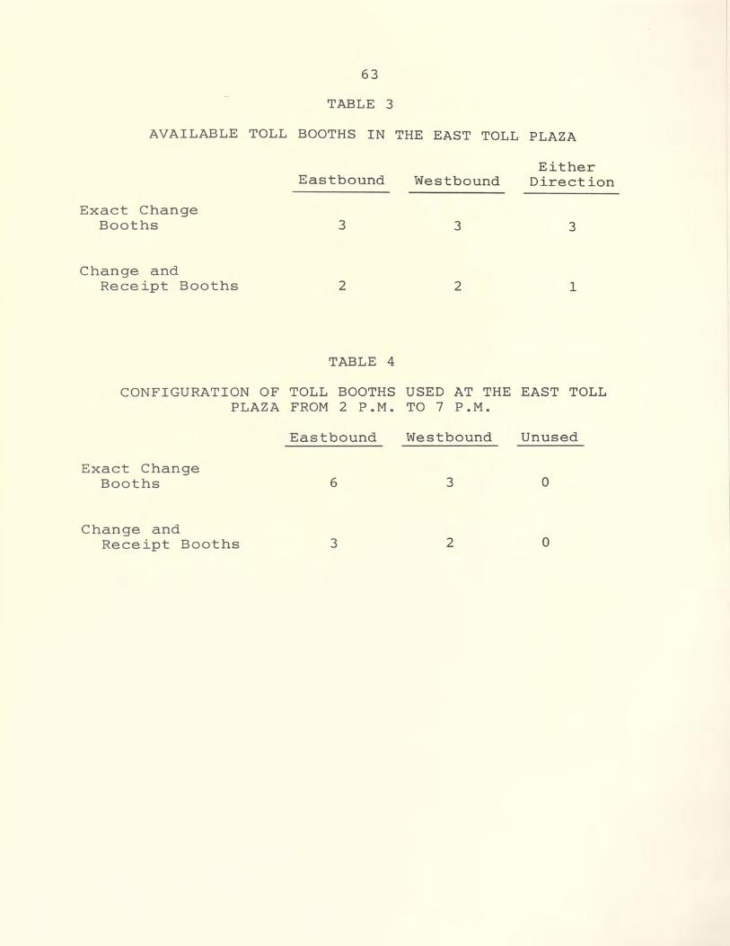
63

TABLE 3

AVAILABLE TOLL BOOTHS IN THE EAST TOLL PLAZA

Exact Change Booths

Change and Receipt Booths

Eastbound

3

2

TABLE 4

Westbound

3

2

Either Direction

3

1

CONFIGURATION OF TOLL BOOTHS USED AT THE EAST TOLL PLAZA FROM 2 P.M. TO 7 P.M.

Exact Change Booths

Change and Receipt Booths

Eastbound

6

3

Westbound Unused

3 0

2 0

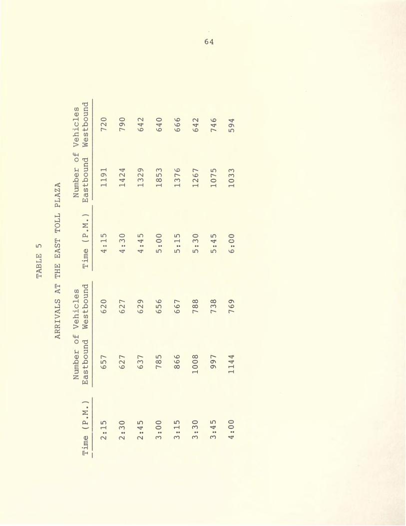
TA

BL

E

5

AR

RIV

AL

S A

T TH

E E

AST

T

OL

L

PLA

ZA

Nu

mb

er

of

Veh

icle

s

Nu

mb

er

of

Veh

icle

s

Tim

e ( P

. M.

) E

ast

bo

un

d

Wes

tbo

un

d

Tim

e ( P

. M.

) E

ast

bo

un

d

West

bo

un

d

2:1

5

65

7

62

0

4:1

5

11

91

7

20

2:3

0

62

7

62

7

4:3

0

14

24

7

90

2:4

5

63

7

62

9

4:4

5

13

29

6

42

3:0

0

78

5

65

6

5:0

0

18

53

6

40

3:1

5

86

6

66

7

5:1

5

13

76

6

66

3:3

0

10

08

7

88

5

:30

1

26

7

64

2

O'I

3:4

5

99

7

73

8

5:4

5

10

75

7

46

~

4:0

0

11

44

7

69

6

:00

1

03

3

59

4

65

A summary of the parameters that were estimated for

this model is:

* the arrival rate, based on Table 5, is assumed to

be exponentially distributed

* the time required to pay the toll at an exact

change booth is an exponential distribution with a

mean of four seconds

* the time required to pay the toll at a change and

receipt booth is an exponential distribution with

a mean of eight seconds

* a vehicle has an average speed of 15 miles per

hour in the 120-foot approach to the toll booth

The Model

Two major assumptions were made when designing this

model:

a) the driver of a vehicle will select the toll

booth he intends to use before he is approximately

120 feet from the toll plaza;

b) the driver will choose a toll booth with the

shortest queue. If he has exact change, he will

still choose the shortest queue, regardless of

whether the toll booth is for exact change or for

change and receipts. If more than one booth has

the shortest queue, he will select the queue

farthest to his right.

66

The model begins with the creation of vehicle

arrivals for eastbound and westbound traffic. The arrival

rates will change with time by use of the TABLES statement

in the experiment section of the model. The arriving

entities trigger the assignment of values for several

variables depending on whether the arrival is eastbound or

westbound. These variables will later be used to select

eastbound or westbound queues.

The entity or vehicle is then assigned an attribute

that will identify the number of axles on the vehicle.

The number of axles will be determined by the ratios shown

in Table 2. If the vehicle has two axles, it is routed to

a statement that determines whether the driver has exact

change. If the vehicle has three or more axles, it is

routed to a statement that searches for the shortest

queue. Once a queue has been selected, the entity waits

for the opportunity to seize a resource (the toll booth).

When the toll booth is seized, the entity will be delayed

the appropriate amount of time necessary to pay the toll

and then release the toll booth. The vehicle will then

resume its travel in the appropriate direction.

Forty-two stations are required for this model.

Fourteen stations are 120 feet from the toll plaza

approach and 14 stations are 120 feet beyond the toll

plaza. These stations are necessary to animate the path

of travel of the entities using Cinema. The remaining 14

67

stations are the toll booths. The layout of the stations

is depicted in Figure 3. While it may seem that the

stations are numbered in an unusual manner, this is

necessary in order to utilize the same subroutine for both

eastbound and westbound traffic.

Several attributes are assigned to each entity during

the course of the simulation. These attributes are

valuable in assembling the data in the summary report that

compiles the outcome of the simulation.

these attributes are described below:

A( 1) = number of axles

A( 2) = time required to pay toll

A( 3) = eastbound ( 2 ) or westbound

A( 4) = time spent in queue

A( 5) = cost of toll

A( 6) = toll booth used

Evaluation

The functions of

( 1)

Several items are required to help ensure that the

simulation of the east toll plaza results in a valid

model. A warm-up period is required to bring the system

to equilibrium before tabulation of data begins. Since

this model was designed to analyze conditions during

evening rush hour, the warm-up period must occur prior to

the peak traffic period, which begins around 3 p.m.

Traffic prior to 3 p.m. is very light at the toll plaza so

SIA 1ION 2'9

SlATION 30

c;TATION 31

STATION !! -

ST A TION l5

MOTM B ST A 1 ION 16 CWH.I.

STATION 19

BOOIH F

68

STATION 2!

----------------ST ATION 1-4

STATION 1.3

STATION 12

STATION I

STATION IO

STA llON 9

STA l!Cf.I 7

STATION 6

Figure 3.

!l001H I

EU.Cl

STATION 27

STATJON 22

STATION t~

EA s T BOUND ~ BOOTH J STATION 25 EX>.Cl

OOC1

80011-t l

0001H W

OUH:E

STATION 2'4

STATJON 23

SlATIOH 21

STATION 20

EAST TOLL PLAZA

Layout of Toll Booth Stations

ST AT lOM I

SH. l))H 2

STATION _.

STATION '47

STATION 4

STATION 40

STATION 39

STATION ~

STATION 37

STATION 35

STATION 3.il

69

it would probably take less than an hour to bring the

system to equilibrium. The time period from 2 p.m. to 3

p.m. would provide an effective warm-up period.

Another measure required for ensuring model validity

is to run several simulations and derive the results from

a statistical summary of all the simulation runs. A

single simulation run would merely provide the modeler

with a single random observation.

Naturally, this model of the east toll plaza cannot

be a valid model without the proper data. Time studies

must be performed to determine the standard time for

paying tolls at the manned and unmanned booths. A study

must also be conducted to determine the anticipated

arrival rates. An excellent test of this model would be

to compare the results of the simulation runs using the

proper data with the real-life conditions at the toll

plaza during the same time period. If the results are

favorable, the modeler can feel secure using forecasts of

future traffic conditions as data for the model.

The results of a valid and credible model are

valuable decision-making tools for planning and designing

the toll booth facilities. This information can be used

for determining whether to construct additional toll

booths, change the toll booth configuration for eastbound

and westbound traffic or keep the present configuration,

70

or whether to increase or decrease the manpower working at

the toll plaza.

Further Applications

Since the expressway system in Orange County is

presently experiencing a large expansion, most of which is

toll roads, there are many potential applications for

using simulation and animation to plan the facilities

required for toll booths and toll plazas. Simulation

models can be used to determine the locations and size of

the new toll booth facilities. A simulation of the entire

expressway system could be used for determining the

various tolls that are required to offset costs and the

impact of toll increases on traffic volume and revenue.

Simulations of existing toll booth facilities using

forecasts of future vehicle traffic can be run to

determine how long the existing facilities will be

adequate and what expansion will be necessary at what

future time.

I feel that a continuation of this effort would make

an excellent semester group project for seniors in

industrial engineering. A group of students with

simulation background would be given the opportunity to

model a real-world system. A group of students with time

study and statistical background could develop the data

necessary for the model. Both groups would find the

71

experience valuable and learn some of the difficulties

encountered when attempting to use textbook solutions to

real-world problems. If such a project is successful,

perhaps the Orlando-Orange County Expressway Authority

would consider sponsoring the project.

BEGIN~

-~' ~0

~0

i0 50 ;0 i0 30 EPiST

10 ~0

10 VEHICLE 20 30 40

*** 50 50 7li

atZi

***

C RC: ~l ~ C:-:: :: ~ :x < ~- ., :~ > ~ ."\; ~:: X --· ~: =.::: r:. '.; ·-· >

CREATE: EX (5, i) -~

~)SS I G N :: P ( 1 ., 1 ) =: ·=- ( :: -: T ~~ 0 ~" >

ASS I G N : ;::• < 5 -: :'.. 0: = ..., .. ;::- ~ ;:::: ~ -;- '"-~ 0 v-, >

72

ASS1GN:A<3>=1; WESTBOUND VARIABLES ASSIGN:X<:!.>=0; ASS 1 G N : X ( 2 > =0 : NE X .. : ( 'v' EH I C._.:.::: ; ASSIGN:n(3)=2~

ASSIGN:X(l>=5; ASS I G:'\:: X ( c' > =·3 ! ASS l G i\J : X { 3 } = 1 5 ~- X ( :~ ; ~

ASSIGN:X(4)=15+X(i>+A(3) ASSIGN:X{5>=13+X(2) ASS I G i'-: : ~~ < 8 > = l ~

IDENTIFY THE TYPE OF VEHICLE ***

ASSIGN: A ( 1 ) --=DP ( ~:::, ~ ) ;

ASSIGN:A<5>=PC1)*~.25~

ASS 1 G N : A ( 3 > =A { :~ > + X ( ··_ > .:; BRAh•C~-: : ... :

:~ = '! A ( 1 ) • :=:CL. 2 ., ;:.~ Y. ~-- ~: ."

h ~ - .'-i., :Z1. 24;::_·f .. . ::~ ~C'.">.i :-!~-:~ ~

E ~- ~::, ~~ &" ~ X t-==~~-:: ··:- :

*11(•*

;:::: 1 ~ D .J , X ~ :~. > ., X ( ~- . ~ : :r_: : ,'-l ( "-. :.~· ·~ .~' > -r ' .. . ··: " _,

ASS I G!'-! ~ H < \.~ :~ ===2; ASS I l.~ r" : :::: < ~::: ) = !?. X { 3, : ~ > :: :\,' .::: -..: . . ( ..:::· ;:.::, y-~"Cj ,_ : __ ) ;

i= : f\ D ,...: ': x ( 5 ) ' x ( 3 ) :: !Y· I ;..: ~ !'•: C.' ( ~· .·' -<·· l\; ·~~ ( "T - :.. '7 ) + ... ~ ~.:.·

q s ?:> I [; 1\.4 : Ci 1: ! .~ > = ~ x ( ·'-' ~ - : ~

EASTBOUND VARIABLES

\)E~ I CLE TYPE TO;_~ REQUIRED

,. . . ... - .•

i0 ;0

'/! )0 )1~

j0

. ~' ~ J~l

;0 ;0

)e· ;0

*~-*

~· ~-:.) ·y ·- .: },_ ~ ..

* .. *

***

ASS I G~: ~~ S>=J-~4~

_-::SS ~ 3 ; · : _.., . ~:A ( 6 ) ;

ASS 1 G~:XC7>=A<1>+13;

C 0 L_: '.'\: - :- : X ( 7 ) , ::. ;

~~~~ASE:BOOT-{Y-14>;

-:--µ~ ;_ ·y·: 1' : ~ ;-.~··:- ( .t.+) ;

ASS!GN:Q(7)=P<6)+28; R 0 L: ··;- E : lJ N ( 6 , 1 > , A ( 7 > :; S TA-;- I 0 ~. , 2 ·3 - 4 2 : D I SP 0 St:: ;

\CH11EMA> EXP~-r T OL.i_S2. EXP TOLL..S2. E

roA l\i Ex per i meY-1t ;::•r•:•cessor 'version ::::;. 1 J)'Tl ght 1985 by Systems Mocel i l""rQ Cor::J.

BEGIN;

73

10 PROJ-ECT, Sl :Ylul_f-; TE. TC:_:.._ ~1 t_nZA, ~ . .J .. Y1A'TTTNGLY, 11/12/37; ?0 DISCRETE, 400, ·3, 42, 42, ·3; 30 REPL 1 cA-:'E., ~~ ., ~~' :t. 81r~e:0 ~ 40 PAF~Atv~ ETERS: -~, ~-. 37:

2,0.97~2,2,0.9819,3,0.5926~4,1.0,5:

4., I:,.. 0:

5' ~~ . :::;t--; : s ., .l; • ::, ., ; _) • ~' ;

5~\ - ~ L ~ ::: E ::.) : 1 -: T I ;-,-: ::: I ~ ~3 v ~; T E >·1 :

Sei CO :_.JN·· ~.~~5:1,#

(?, # .-3, #

4,#

5,# s., #

;- t-; RU

TdRLJ ; -:-~ R i.J :- ~-1 r~U

-,- ,...; f~~

Bou-,·:_, Doc ·~ -:-

BDC ·- :., f 1 0 l.~. -:·· ,_,

A: B.:: c;:

.-;:,, ~;

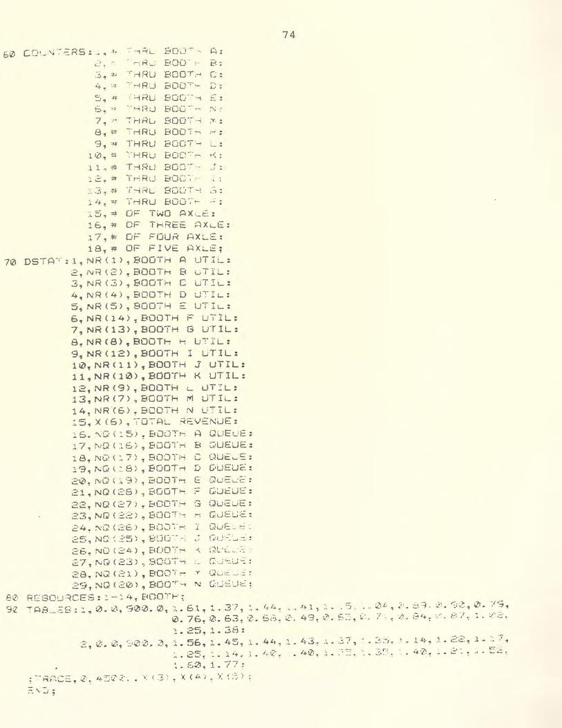
·4., 4

=•., ·"F

E~, ·~ ::s

7., J"~

8., :;:!'

9, :r-J

l lil., ~

11" :~

:.:. .I+' :i:r

c-; ~L - . R-__ : 1-·:'

. ,. dRU

~f RU

~ ;:~u

'-i r~ :J

ii-J RL __, .. riRU

THRU ';-HRU

Tri RU T r--; R ~_: -1- :--1 ;~ L '.

-;'rlRU

:-:.o~j -- ~I

E<oo ··· r-- t~

BOOT :-i c Boo--~ ~-'\

/,,_•

BOC.: .. - :-1 ··-BOC

_ .. ;.~

BOO --· --1 ;Y-;

Boo-;· .'-\ ;-

8DOT '_, c__

t.-=.oc-:-- t-' ~<

Boe:;-'· :-- ·r

"' Boe-.· ·' 8DC:1T~:

.-'--,

EtOO -··· ·-.. -

l5.,~ OF TWO AX~E:

:

. ::

:

.:

:

:

.: ~

:

:

:

.

16.,# OF ThREE AXLE: i7,# OF FOU~ AX~E: i8,~ OF FIVE AX~~~

70 DSTA-, .. : 1., NR ( 1 >., BOOTH A UT l ~-: 2,NR(2>,BOOTh 8 uTlL: 3.,NRC3>,BOOTH CUTI~: 4.,NR(4),BOOTH D LlTIL: 5,NR<5>.,8007H - UTIL: 6,NR(14)~BOOTH F UTIL: 7,NR<13>,BOOTH G UTIL: 8,NRC8),B00Th ~ LTlL: 9,NR<l2>,BOOTH 1 UT1L: 10,NR(ll),BOOTH J UTIL: 11,NR(10>,BOOTH K UTlL: i2,NR(9).,800TH L uT:L: 13,NR<7>?BOOTH ~ LlTIL: 14,NR16>~BOOTH N UTIL: :5.,XC5>,70TAL ~EVENUE: 1 S .. . "-~Q \ l =· > ! fq.J:..JT~. A QUEi_>f:; l 7, r,1Q ~ :L 6 >? BuOTri 8 ~;uF.::UE:

iB, NG'1 ( :-.. 7), BOOTH C DUtL..~:

l9,NQC:8),B00Trl D OUEU~~ 20!NOC~9),800T~ E OuE~~: 21,NQ(2S>,8GGT~ Q~~UE.:

22,NQC27)!BOOTH G QuEGE: 23, NQ ( 2~~ >., 8DCT :-~ , . CLJE:u:::::: 2 4 ~ :--..·G < ~:::E.) ., 800 ; .. .-; i. Q~-1~ :_ ~.-: :

25, NS'. ~ :=:5) ., :8UC .. _--: C·c/-~ ~_, _::: =

26~ NO { 2-'4· ) , BOO .. _'.>-• J, :~L ' t-_" ::..~ :·

27, NQ < 2~3) ') BCGT;...; 2 e ., N Q < ~~ l > , Boen ~ ;:::9, NG < 21Zd , Boo-r· ·-1 ~

74

8tZ: RESC~~:~cES: ~ - ::. 4, 8COT~· ~ sz ; A ... ~ :_ o=: ~~ : :l. ., 0., !,(~, 90 0 • 0, :~. • 6 1 '! :".. ., 3 7 ., ~ w (,\ /_:. ~ ' , ,(~ 1 'J ,_ n · - ~) ,' · • " ~) j_. ' ;-: • ::.• :1 - :/! • ':; ~?.: ') 0 H · ;; (:-; 'J

0.. 7 6 ! ~Zl. 6 3 ~ ,z • S (::1 ~ ~:· . 4 '3 ~ r.? ~ ~- ~:_:.: , ~ ~ _ ?"._ ~ ,~~ , E• ..... -: '. ,-~ . e. "/ ·: ::.. . :/: ~:.:· ~

l. 25., 1,. :38: ;;:~, :L>. ~;, ';)(-:'.i). ;~, :L • 56, ], • 45., \ • .4.£~~ !_ ,. 43~ ,;, n .37 1 :' . H ::<::i~ 1

_t.L). ".' ~- H ;:::;:::., 1 ~ :·~ './.,

·_ • .(~0 ~ " .i.. ... ·· · ·--:

= .·.::

:'.. .. S7-l, 1 .. Tl : -:- ~ ~-::~ C ·== , :Z: a: '~- 5 ~"'· .J:· . • \ ( .°3 -~ ., ."' ( LJ. ·1 •.• X 1

: :·-:: .. • ) ~-

~' ::J;

SIMJLA~E 70L~ ~~AZA w J rf)AT T 1 ~!m_ v

1 ~ /: 2 / 1'3B7

~noed at ti '"e :

er 1 de~1t if i er Average

75

Standarc Minimum De-..,.. i at 2- <::<r '.Jal ue·

Maximum Value

Number. c«f Obs ..

-----------------------------------------------------·---------------------- -

er l de rr t i -f i er

35.85258 .00000 723.07620

Discrete Change Variables

Average Standard Minimum Devi at i e<r1 Val t.te

Maximum Value

33:.S7

---------------------------------------------------------------------------.i

BOOTH A UTIL . 89 . 32 • 00 1. 00 18000.00

2 BOOTH B UTIL . 85 .. 36 • 00 1. 00 18000.;00

3 BOOTH c UTIL . 61 . 4·3 . 00 1. 00 18000. 00

4 BOOTH D UTlL . 65 • 48 • 00 1. 00 18000 .. >2U2'

5 BOOTH E UTIL . 71 . 46 .00 1. 00 18000. 00

b BOOTH F UT!L . 62 . 49 • 00 1. 00 18000. 00 .., BOOTH G UTIL . 6tZI . 49 • 00 1. 00 18000. 00 I

8 BOOTH H UTIL . 76 . ,t."':i' . 00 1. 00 18000 .. 00 • .....J

9 BOOTH I UTIL . 56 " 50 . 012! 1. 00 l 800e~. 00

lei BOOTH J UTIL r:::--· 5:2: .. 00 1. 00 18000. 0~) . ...J~ ..

' ' BOOTH K UTIL . 48 . =<0 . 00 1. • 00 18000 .. 00 . ~ I ·- 1 BOOTH L UT-1L .. 43 .. 50 - 1210 .. 00 18000 . 0Q1 u::.

..... ~3 BOOTH M UTIL . 79 .. 41 . 00 1 .. 00 18000. 00

\ L1 800-! '.--1 N LJTIL .. 85 .. 36 -00 ..... ill0 18000. 00

15 TOTAL REVENUE 8294. 14 c:=-- '· C' 2·3 . 00 1 7023. ·::>C:- 18000. 0Q~ .._1~.l.i·._!.. ~...s

l. 6 BOOTH A QUEUE 3. 25 4. 0E. .00 22.00 18000. 00

17 BOOTH 8 QUEUE ·=· 89 3. ·35 . 00 ·:::>·::. 00 18000. 0lli '-. ...... ......

i .s Boo-:- ;-1 c QU~wE - 48 .. 94 . 00 B .. 00 1 E~000 .. ~210

. ' BO=: i- ~ . ~ QUEUE . 59 .:.. . 03 .. t.llll 7. 00 ::.. 8000. 00

.• -2tl ~~oo-~· ~""'. E C:UELlE 7-;. 1 .. 1 c-. eiei 8. \Z10 1 EH~1 ~~ il< • 0:21 . ~, . i. ~-\ .

, . 80 ·=7~~ C)LJEUE = ·-· 1 • ·~ •· tl:tll 10 .. Ille. :! 800tl1 .. lli :Z: ,_ - . - - '-'...::.. ..... ... .

BDo-- ·,_J c; QUEU:=:: 47 .. 17 :Z10 10. 00 18000. 00 L:C_

.. ..

C~ 3 8.:JC• --:·>-1 QLJEUE ·: =. 87 -- -r=- 23 00 81. 00 :.: ae,00. fZ:C > .... ._; .. c-..: • ..

~~4 BOOTH 1 QUEUE . 41 . 1. 12 . 00 10. 00 18000 .. eie\ -.c BOOTH J QUEUE 37 1. 12 . 00 9 .. 00 1 se~00 .. 0 ,-,.. c._1 . .... _

2[. BCJOT~ f..t.; QUEUE ~.., 1. 01 A 0er 9. 0e : 8("llZ· J.~ .. 2:1? A ..;;i ...

G)UEUE 2'3 e· Q! 1Z 9 .. 00 :. B00t2<. ~ ... ,:~ 27 BOO Tri ' .. ... . ' .... . ·-

OUE~JE .: E. 0. r-\ .-. c:- ~::~ s '2:0 81 .. 00 1 8~~i.?iQ: A 2_1 .:;• ;~8 BOOTH ~ L..i

.;--_.__,,. ~

2'3 BOOT~ N QUEUE i 6 .. 33 ·::. '-'. 3~1 Q;:i~ E1 l. ,Z,0 ::. 8000. :J:.:(;-~- "-' .. ..

76

L_ 1 rn i "t:

-. # Tl-~ RU 800~ :-1 - ~ ~~ - 7iC, I l'"l f i Y: i t E?

·· - rf ........ ~ - ' . . ;- :-< L.J Boo-·-: ··-i 8 2 ::=: :214 .t ·n -f i "!'": .~ t: e -rt Ti-:?U 8iJDT ·"". .~ 26'3S· .!. n r ~- .-. ·::e ·-1~ ii-iRU Boo-:· ··-1 r, :=:948 l nf -1 ·~: .1 ~; e "+ 4J

= # Th RU Boo-:-:-j - 3~:::41 I l'"s·f i Y-:-.:. te --~' --c. # THRU BOOT;-l ;-..J 1334 I r1f i r1 it e 1-J

7 # THRU aoo:H ~ ::.883 I rs f i 1"1 i t e ,9 :;~ THRU BOOTH )-; 1799 I 's'"'s f i r-: :l t e ·3 # THRU BOOTH i_ :i. '31 7 I l'"1f i l""i i te

10 :;~ THRU BOOT~ _--( ~:152 I r1 f i ..,..: i. t e

~ - # T!-!RU BOOT~ J 2289 I n-f i l"11 t e .... - ,

:~; irlRU BOOTH 'T ;~ l'.t-83 I r1 ·f i ~1 i t e .. :_ .L

13 # THRU BOOTH ~J C'623 I r1'f :i rite

14 # THRU BOOT'.-4 F ;=:82''3 1 nf i Y1 i. t e

15 # OF TWO AXLE 32255 I rf i l'"1 it e

16 # OF THREE AX~-E 324 I·f"sfinite

17 # OF FOUR AXLE 329 Infirsite

18 # OF FIVE AXLE 259 I's'"'s-finite

~Ul'"I Ti rne 55 Mi l'"11_<t e ( s) and 40 Secc1l'"1ci ( s)

Stoo ~rogram terminated.

BIBLIOGRAPHY

Bradley, Stephen P. Applied Mathematical Programming. Reading, Massachusetts: Addison-Wesley Publishing Company, 1977.

Carson, John S. "Convincing Users of Model's Validity is Challenging Aspect of Modeler's Job" Industrial Engineering (June 1986): 74-85.

Cobbin, Phillip. "Simple 1: A Simulation Environment for the IBM PC" Modeling and Simulation on Microcomputers (1986): 243-248.

Cox, Springer, and Cox, Alice J. "GPSS/PC: A User Oriented Simulation System" Modeling and Simulation on Microcomputers (1985): 48-50.

Dao, Thien-My. "A Microcomputer Software for Probabilistic Modeling and Simulation of PERT" Modeling and Simulation on Microcomputers (1985): 111-113.

Grant, John W., and Weiner, Steven A. "Factors to Consider in Choosing a Graphically Animated Simulation System" Industrial Engineering (August 1986): 37-68.

Haider, S. Wali, and Banks, Jerry. "Simulation Software Products for Analyzing Manufacturing Systems" Industrial Engineering (July 1986): 98-103.

Hitomi, K. Manufacturing Systems Engineering. London: Taylor & Francis Ltd., 1979.

Kelton, David W. Statistical Analysis Methods Enhance Usefulness, Reliability of Simulation Models" Industrial Engineering (September 1986): 74-84.

Law, Averill M. "Introduction to Simulation: A Powerful Tool for Analyzing Complex Manufacturing Systems" Industrial Engineering (May 1986):

Law, Averill M. "Statistical Analysis of Simulation Output Data" Operations Research (1983): 983~1029.

77

78

Law, Averill M. and Kelton, w. D. Modeling Analysis. New York:

Simulation and McGraw-Hill, 1982.

Lilegdon, William R., and O'Reilly, Jean J. "SLAM II for Microcomputers" Modeling and Simulation on Microcomputers (1985): 31-36.

Mackulak, Gerald T. SIMFACTORY with Animation User's Manual. Los Angeles: CACI, 1986.

Micro Analysis and Design, Inc. Micro SAINT Technical 1987. Specifications Release 3.0:

Pegden, C. Dennis. Introduction to SIMAN. Systems Modeling Corp., State College, PA, 1986.

Pence, James A., and Finkel, David. "Modeling a Computer Simulation with SIMAN on the IBM Personal Computer" Modeling and Simulation on Microcomputers (1984): 107-111.

Systems Modeling Corp. Cinema System for Simulation and Animation: 1986.

Welch, P. D. Results" Orlando:

"The Statistical Analysis of Simulation The Computer Performance Modeling Handbook.

Academic Press, 1983.