Applications of Renormalization Group Methods in Nuclear ...ntg/8805/slides/HUGS_2014_furn... ·...

Applications of Renormalization GroupMethods in Nuclear Physics – 1

Dick FurnstahlDepartment of PhysicsOhio State University

HUGS 2014

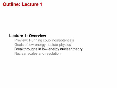
Outline: Lecture 1

Lecture 1: OverviewPreview: Running couplings/potentialsGoals of low-energy nuclear physicsBreakthroughs in low-energy nuclear theoryNuclear scales and resolution

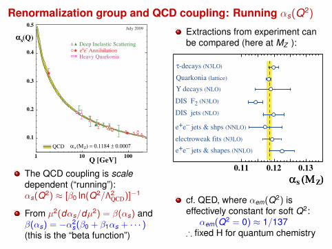
Renormalization group and QCD coupling: Running αs(Q2)

QCD α (Μ ) = 0.1184 ± 0.0007s Z

0.1

0.2

0.3

0.4

0.5

αs (Q)

1 10 100Q [GeV]

Heavy Quarkoniae+e– Annihilation

Deep Inelastic Scattering

July 2009

The QCD coupling is scaledependent (“running”):αs(Q2) ≈ [β0 ln(Q2/Λ2

QCD)]−1

From µ2(dαs/dµ2) = β(αs) andβ(αs) = −α2

s(β0 + β1αs + · · · )(this is the “beta function”)

Extractions from experiment canbe compared (here at MZ ):

0.11 0.12 0.13

α (Μ )s Z

Quarkonia (lattice)

DIS F2 (N3LO)

τ-decays (N3LO)

DIS jets (NLO)

e+e– jets & shps (NNLO)

electroweak fits (N3LO)

e+e– jets & shapes (NNLO)

Υ decays (NLO)

cf. QED, where αem(Q2) iseffectively constant for soft Q2:

αem(Q2 = 0) ≈ 1/137∴ fixed H for quantum chemistry

Running QCD αs(Q2) vs. running nuclear Vλ(k , k ′)

QCD α (Μ ) = 0.1184 ± 0.0007s Z

0.1

0.2

0.3

0.4

0.5

αs (Q)

1 10 100Q [GeV]

Heavy Quarkoniae+e– Annihilation

Deep Inelastic Scattering

July 2009

The QCD coupling is scaledependent (cf. low-E QED):αs(Q2) ≈ [β0 ln(Q2/Λ2

QCD)]−1

Different Hamiltonians? Do youget different answers from thesame Feynman diagrams withαs(µ2

1) and αs(µ22)?

Vary scale (“resolution”) with RG=⇒ diff. eq. for potential V

Scale dependence: RG running ofinitial potential with scale λ(decoupling or separation scale)

But all are (NN) phase equivalent!(predict the same NN cross sections)

Shift contributions between interactionand sums over intermediate states

Outline: Lecture 1


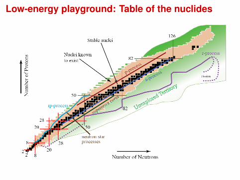
Low-energy playground: Table of the nuclides

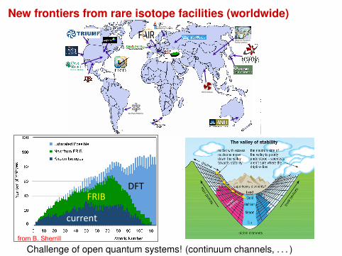
New frontiers from rare isotope facilities (worldwide)Isotope science: XXI scienceHeavy Ion Research Facility Lanzhou

VECC Kolkata

Sao Paulo Pelletron

51

Asymptotic freedom ?

from B. Sherrill

DFT$FRIB$

current$

Challenge of open quantum systems! (continuum channels, . . . )

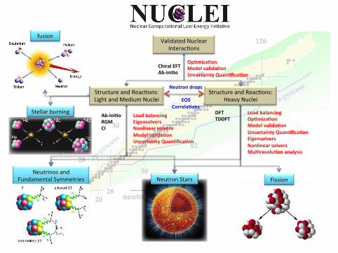
Validated Nuclear Interac/ons

Structure and Reac/ons: Light and Medium Nuclei

Structure and Reac/ons: Heavy Nuclei

Chiral EFT Ab-‐ini/o

Op/miza/on Model valida/on Uncertainty Quan/fica/on

Neutron Stars Neutrinos and

Fundamental Symmetries

Ab-‐ini/o RGM CI

Load balancing Eigensolvers Nonlinear solvers Model valida/on Uncertainty Quan/fica/on

DFT TDDFT

Load balancing Op/miza/on Model valida/on Uncertainty Quan/fica/on Eigensolvers Nonlinear solvers Mul/resolu/on analysis

Stellar burning

fusion

Neutron drops

EOS Correla/ons

Fission

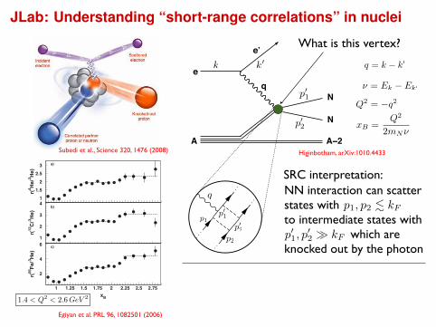
JLab: Understanding “short-range correlations” in nucleiCorrelations in nuclear systems

A!1A

q

A

q

e e

e’ e’

a) b)

A!2

N

NN

FIGURE 1. The simple goal of short-range nucleon-nucleon correlation studies is to cleanly isolate diagram b) from a).Unfortunately, there are many other diagrams, including those with final-state interactions, that can produce the same final state asthe diagram scientists would like to isolate. If one could find kinematics that were dominated by diagram b) it would finally allowelectron scattering to provide new insights into the short-range part of the nucleon-nucleon potential.

For A(e,e’p) reactions, one can determine not only the energy and moment transferred, but also the energy and

momentum of the knocked-out nucleon. The difference between the transferred and detected energy and momentum

is referred to as the missing energy, Emiss and missing momentum, pmiss, respectively. From the theoretical works on

how short-range nucleon-nucleon correlations effects the momentum distribution of nucleons in the nucleus [6], it

is clear one must probe beyond the simple particle in an average potential motion of the nucleon in the nucleus of

approximately 250 MeV/c in order to observe the effects of correlations.

With the construction of the Jefferson Lab Continuous Electron Beam Facility (CEBAF) [7], it was possible to

do high-luminosity knock-out reactions in ideal quasi-elastic kinematics into the pmiss > 250 MeV/c region. In the

early Jefferson Lab knock-out reaction proposals, such as E89-044 3He(e,e’p)pn and 3He(e,e’p)d, these kinematics

were argued as the key to cleanly observe the effects of short-range correlations. And while final results of the

experiments were clearly effected by the presence of correlations, the magnitude of the cross sections in the high

missing momentum region was dominated by final-state interaction effects [8, 9]. Equally striking was the D(e,e’p)n

data from CLAS taken at Q2 > 5 [GeV/c]2 in xB < 1 kinematics [10]. Here it was shown that meson-exchange currents,final-state interaction, and delta-isobar configurations mask cleanly probing nucleon-nucleons even at extremely high

Q2 in xB < 1 kinematics.

NUCLEAR SCALING

With both the xB < 1 and xB = 1 kinematics practically ruled out for ever being able to cleanly probe short-range

correlations; there is only one region left to explore: xB > 1. This is a special region, since it is kinematically

forbidden for a free nucleon, and thus seems to be a natural place to observe effects of multi-nucleon interactions.

These kinematics were probed with limited statistics at SLAC [11] and the plateaus in the per nucleon ratios, r(A/d),

were claimed at to be evidence for short-range correlations [12].

In 2003, CLAS published high statics data in the same kinematic region. The results clearly showed that the plateaus

could only be seen for Q2 > 1 [GeV/c]2 and xB > 1 kinematics [13] as predicted by Frankfurt and Strikman [14]. But

plateaus alone are not evidence for correlations, just evidence that the functional form of the cross section is the same

for the two nuclei; so data was taken the xB > 2 region. By logic, if 1< xB < 2 is a region of two-nucleon correlations,

then the xB > 2 region should be dominated by three-nucleon correlations. The CLAS Q2 > 1 and xB > 2 experiment

reported observing a second scaling plateau as shown in Fig. 2 [15]. Preliminary results of Hall C high precision data

have shown roughly the same magnitude for these plateaus as CLAS and shown that there is no Q2 dependence in the

2< Q2 < 4 [GeV/c]2 range [16, 17].

Subedi et al., Science 320, 1476 (2008)

would demonstrate the presence of 3-nucleon (3N) SRCand confirm the previous observation of NN SRC.

Note that: (i) Refs. [5,6] argue that the c.m. motion of theNN SRC may change the value of a2 (by up to 20% for56Fe) but not the scaling at xB < 2. For 3N SRC there areno estimates of the effects of c.m. motion. (ii) Final stateinteractions (FSI) are dominated by the interaction of thestruck nucleon with the other nucleons in the SRC [7,8].Hence the FSI can modify !j, while such modification ofaj!A" are small since the pp, pn, and nn cross sections atQ2 > 1 GeV2 are similar in magnitudes.

In our previous work [6] we showed that the ratiosR!A; 3He" # 3!A!Q2;xB"

A!3He!Q2;xB" scale for 1:5< xB < 2 and 1:4<

Q2 < 2:6 GeV2, confirming findings in Ref. [7]. Here werepeat our previous measurement with higher statisticswhich allows us to estimate the absolute per-nucleon prob-abilities of NN SRC.

We also search for the even more elusive 3N SRC,correlations which originate from both short-range NNinteractions and three-nucleon forces, using the ratioR!A; 3He" at 2< xB $ 3.

Two sets of measurements were performed at theThomas Jefferson National Accelerator Facility in 1999and 2002. The 1999 measurements used 4.461 GeV elec-trons incident on liquid 3He, 4He and solid 12C targets. The2002 measurements used 4.471 GeVelectrons incident on asolid 56Fe target and 4.703 GeV electrons incident on aliquid 3He target.

Scattered electrons were detected in the CLAS spec-trometer [9]. The lead-scintillator electromagnetic calo-rimeter provided the electron trigger and was used toidentify electrons in the analysis. Vertex cuts were usedto eliminate the target walls. The estimated remainingcontribution from the two Al 15 "m target cell windowsis less than 0.1%. Software fiducial cuts were used toexclude regions of nonuniform detector response. Kine-matic corrections were applied to compensate for driftchamber misalignments and magnetic field uncertainties.

We used the GEANT-based CLAS simulation, GSIM, todetermine the electron acceptance correction factors, tak-ing into account ‘‘bad’’ or ‘‘dead’’ hardware channels invarious components of CLAS. The measured acceptance-corrected, normalized inclusive electron yields on 3He,4He, 12C, and 56Fe at 1< xB < 2 agree with Sargsian’sradiated cross sections [10] that were tuned on SLAC data[11] and describe reasonably well the Jefferson Lab Hall C[12] data.

We constructed the ratios of inclusive cross sections as afunction of Q2 and xB, with corrections for the CLASacceptance and for the elementary electron-nucleon crosssections:

r!A; 3He" # A!2!ep % !en"3!Z!ep % N!en"

3Y!A"AY!3He"R

Arad; (2)

where Z and N are the number of protons and neutrons innucleus A, !eN is the electron-nucleon cross section, Y isthe normalized yield in a given (Q2; xB) bin, and RA

rad is theratio of the radiative correction factors for 3He and nucleusA [see Ref. [8] ]. In our Q2 range, the elementary crosssection correction factor A!2!ep%!en"

3!Z!ep%N!en" is 1:14& 0:02 for C

and 4He and 1:18& 0:02 for 56Fe. Note that the 3He yieldin Eq. (2) is also corrected for the beam energy differenceby the difference in the Mott cross sections. The corrected3He cross sections at the two energies agree within $ 3:5%[8].

We calculated the radiative correction factors for thereaction A!e; e0" at xB < 2 using Sargsian’s upgradedcode of Ref. [13] and the formalism of Mo and Tsai [14].These factors change 10%–15% with xB for 1< xB < 2.However, their ratios, RA

rad, for 3He to the other nuclei arealmost constant (within 2%–3%) for xB > 1:4. We appliedRArad in Eq. (2) event by event for 0:8< xB < 2. Since there

are no theoretical cross section calculations at xB > 2, weapplied the value of RA

rad averaged over 1:4< xB < 2 to theentire 2< xB < 3 range. Since the xB dependence of RA

radfor 4He and 12C are very small, this should not affect theratio r of Eq. (2). For 56Fe, due to the observed small slopeof RA

rad with xB, r!A; 3He" can increase up to 4% at xB #2:55. This was included in the systematic errors.

Figure 1 shows the resulting ratios integrated over 1:4<Q2 < 2:6 GeV2. These cross section ratios (a) scale ini-tially for 1:5< xB < 2, which indicates that NN SRCs

a)

r(4 H

e/3 H

e)

b)

r(12

C/3 H

e)

xB

r(56

Fe/3 H

e)

c)

1

1.5

2

2.5

3

1

2

3

4

2

4

6

1 1.25 1.5 1.75 2 2.25 2.5 2.75

FIG. 1. Weighted cross section ratios [see Eq. (2)] of (a) 4He,(b) 12C, and (c) 56Fe to 3He as a function of xB for Q2 >1:4 GeV2. The horizontal dashed lines indicate the NN (1:5<xB < 2) and 3N (xB > 2:25) scaling regions.

PRL 96, 082501 (2006) P H Y S I C A L R E V I E W L E T T E R S week ending3 MARCH 2006

082501-3

Higinbotham, arXiv:1010.4433

Egiyan et al. PRL 96, 1082501 (2006)

What is this vertex?

k k q = k − k

ν = Ek − Ek

p1

p2

p1

SRC interpretation:

NN interaction can scatter states withto intermediate states with which are knocked out by the photon

p1, p2 kF

How to explain cross sections in terms of low-momentum interactions?

Vertex depends on the resolution!

q

p1

p2

p1, p2 kF

p2

1.4 < Q2 < 2.6 GeV 2

Q2 = −q2

xB =Q2

2mNν

Outline: Lecture 1


Historical perspective: JLab experimentalist [L. Weinstein (2012)]

Comprehensive Theory Overview

Nuclear Theory - circa 2000

Nuclear Theory - today: 1, 2, 3, … 12, … many

Historical perspective: “Ab initio” structure 10–15 years ago

Figure from the RIA (now FRIB) white paper (2000)

5

82

50

28

28

50

82

2082

28

20

126

A=10

A=12 A~60

Density Functio

nal Theory

Selfconsis

tent Mean Field

Ab initiofew-body

calculations No-Core Shell Model G-matrix

r-process

rp-process

0Ñω ShellModel

Limits of nuclearexistence

pro

tons

neutrons

Many-body approachesfor ordinary nuclei

Figure 2: Top: the nuclear landscape - the territory of RIA physics. The black squares represent the stable nuclei and the nuclei with half-lives comparable to or longer than the age of the Earth (4.5 billion years). These nuclei form the "valley of stability". The yellow region indicates shorter lived nuclei that have been produced and studied in laboratories. By adding either protons or neutrons one moves away from the valley of stability, finally reaching the drip lines where the nuclear binding ends because the forces between neutrons and protons are no longer strong enough to hold these particles together. Many thousands of radioactive nuclei with very small or very large N/Z ratios are yet to be explored. In the (N,Z) landscape, they form the terra incognita indicated in green. The proton drip line is already relatively well delineated experimentally up to Z=83. In contrast, the neutron drip line is considerably further from the valley of stability and harder to approach. Except for the lightest nuclei where it has been reached experimentally, the neutron drip line has to be estimated on the basis of nuclear models - hence it is very uncertain due to the dramatic extrapolations involved. The red vertical and horizontal lines show the magic numbers around the valley of stability. The anticipated paths of astrophysical processes (r-process, purple line; rp-process, turquoise line) are shown. Bottom: various theoretical approaches to the nuclear many-body problem. For the lightest nuclei, ab initio calculations (Green’s Function Monte Carlo, no-core shell model) based on the bare nucleon-nucleon interaction, are possible. Medium-mass nuclei can be treated by the large-scale shell model. For heavy nuclei, the density functional theory (based on selfconsistent mean field) is the tool of choice. By investigating the intersections between these theoretical strategies, one aims at nothing less than developing the unified description of the nucleus.

Ab initio: Only up to 12C (GFMC and NCSM with NN+3N)

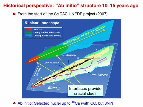
Historical perspective: “Ab initio” structure 10–15 years ago

From the start of the SciDAC UNEDF project (2007)

Interfaces provide crucial clues

dimension of the problem

Ab initio: Selected nuclei up to 40Ca (with CC, but 3N?)

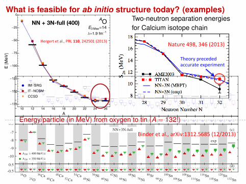
What is feasible for ab initio structure today? (examples)

H. Hergert - The Ohio State University - “Nuclear Structure & Reactions: Experimental and Ab Initio Theoretical Perspectives”, TRIUMF, 02/19/2014

10 12 14 16 18 20 22 24 26175

150

125

100

75

50

25

0

A

EMeV

AOE3Max141.9 fm1

IMSRG

10 12 14 16 18 20 22 24 26175

150

125

100

75

50

25

0

A

EMeV

AOE3Max141.9 fm1

IMSRG

ITNCSM

10 12 14 16 18 20 22 24 26175

150

125

100

75

50

25

0

A

EMeV

AOE3Max141.9 fm1

IMSRG

ITNCSM

CCSD

10 12 14 16 18 20 22 24 26175

150

125

100

75

50

25

0

A

EMeV

AO

E3Max141.9 fm1

IMSRG

10 12 14 16 18 20 22 24 26175

150

125

100

75

50

25

0

A

EMeV

AO

E3Max141.9 fm1

IMSRG

ITNCSM

10 12 14 16 18 20 22 24 26175

150

125

100

75

50

25

0

A

EMeV

AO

E3Max141.9 fm1

IMSRG

ITNCSM

CCSD

NN + 3N-full (400)

Phys. Rev. Lett. 110, 242501 (2013)

Results: Oxygen Chain

• reference state: number-projected Hartree-Fock-Bogoliubov vacuum (pairing correlations)

• consistent results from different many-body methods

NN + 3N-ind.

exp.

Hergert&et&al.,&PRL&110,&242501&(2013)&

Two-neutron separation energiesfor Calcium isotope chain

Exciting advances for neutron-rich nuclei

3N forces key to explain 24O as heaviest oxygen isotope Otsuka, Suzuki, Holt, Schwenk, Akaishi, Phys. Rev. Lett. 105, 032501 (2010).

predicted increased binding for neutron-rich calcium

confirmed in precision Penning trap exp.

5! and 3! deviation in 51,52Ca from AME TITAN collaboration + Holt, Menendez, Schwenk, submitted.

Impact on global predictions?

Nature'498,'346'(2013)'

Theory'preceded'accurate'experiment'

Energy/particle (in MeV) from oxygen to tin (A = 132!)

-10

-9

-8

-7

-6NN+3N-induced

! N3LO! N2LOopt

(a)

exp

-0.5

0.5 (b)

-10

-9

-8

-7

.

E/A

[MeV

]

NN+3N-full

! Λ3N = 400 MeV/c

! Λ3N = 350 MeV/c

(c)

exp

16O24O

36Ca40Ca

48Ca52Ca

54Ca48Ni

56Ni60Ni

62Ni66Ni

68Ni78Ni

88Sr90Zr

100Sn106Sn

108Sn114Sn

116Sn118Sn

120Sn132Sn

-0.5

0.5 (d)

Binder'et'al.,'arXiv:1312.5685'(12/2013)'

Outline: Lecture 1


Standing on the shoulders of giants . . .

Steven Weinberg (1933– )Nobel Prize 1979

electroweak theory (GWS), . . .

effective field theory (EFT)applied to nuclear physics

Kenneth G. Wilson (1936–2013)Nobel Prize 1982

renormalization group (RG)and critical phenomena, . . .

similarity RG

=⇒ Conceptual basis for changing “resolution” and tools to do it!

Connecting degrees of freedom with EFT and RG

Res

olut

ion

scale&separa)on&

DFT

collective models

CI

ab initio

LQCD

constituent quarks

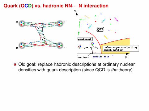
Quark (QCD) vs. hadronic NN· · ·N interaction

!"#$%&'%()*+($"#,)-.,("

!"%/01 %&)-,.234 5 6'.7& "' #$ 8!949 :0;< =>00?@3A4A5A6'.7&)"')#$AB)8!949B):0;<)=>00?@A

C3>D %&)-,.2!AEAF%,%*G#)"')#$AB)8!951B)1H)=>00;@A

IA)J&K%%B)6A)C.7%B)LA)M#'&+/#B)8KN&A)!"OA)P"''A)99, <::<<>)=:<<Q@L"*&.,)-.,(")-,.2)PR9ST)K''UTVV#,W%OA.,GVU/-V<0<1A;?0QOld goal: replace hadronic descriptions at ordinary nuclear

densities with quark description (since QCD is the theory)

New goal: use effective hadronic dof’s systematically

Seek model independence and theory error estimatesFuture: Use lattice QCD to match via “low-energy constants”

Need quark dof’s at higher densities (resolutions) wherephase transitions happen or at high momentum transfers

Quark (QCD) vs. hadronic NN· · ·N interaction

!"#$%&'%()*+($"#,)-.,("

!"%/01 %&)-,.234 5 6'.7& "' #$ 8!949 :0;< =>00?@3A4A5A6'.7&)"')#$AB)8!949B):0;<)=>00?@A

C3>D %&)-,.2!AEAF%,%*G#)"')#$AB)8!951B)1H)=>00;@A

IA)J&K%%B)6A)C.7%B)LA)M#'&+/#B)8KN&A)!"OA)P"''A)99, <::<<>)=:<<Q@L"*&.,)-.,(")-,.2)PR9ST)K''UTVV#,W%OA.,GVU/-V<0<1A;?0Q

Old goal: replace hadronic descriptions at ordinary nucleardensities with quark description (since QCD is the theory)New goal: use effective hadronic dof’s systematically

Seek model independence and theory error estimatesFuture: Use lattice QCD to match via “low-energy constants”

Need quark dof’s at higher densities (resolutions) wherephase transitions happen or at high momentum transfers

Low resolution makes physics easier + efficient

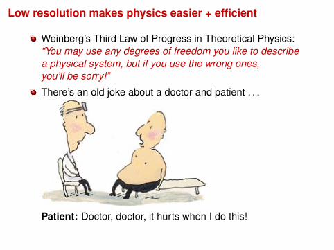
Weinberg’s Third Law of Progress in Theoretical Physics:“You may use any degrees of freedom you like to describea physical system, but if you use the wrong ones,you’ll be sorry!”

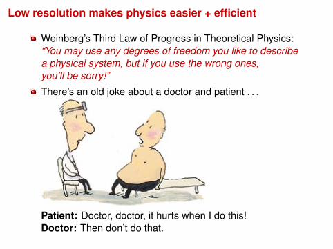
There’s an old joke about a doctor and patient . . .

Patient: Doctor, doctor, it hurts when I do this!Doctor: Then don’t do that.




Patient: Doctor, doctor, it hurts when I do this!

Doctor: Then don’t do that.




Patient: Doctor, doctor, it hurts when I do this!Doctor: Then don’t do that.

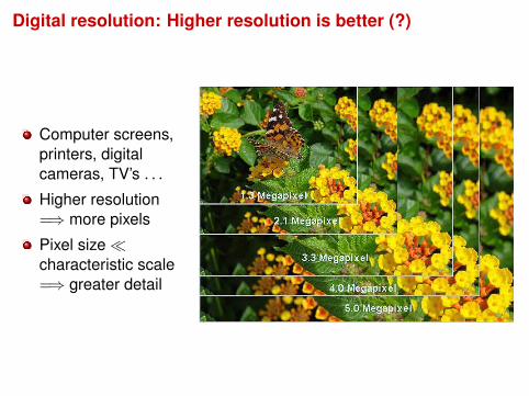
Digital resolution: Higher resolution is better (?)

Computer screens,printers, digitalcameras, TV’s . . .

Higher resolution=⇒ more pixels

Pixel sizecharacteristic scale=⇒ greater detail

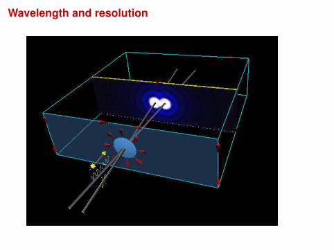
Diffraction and resolution

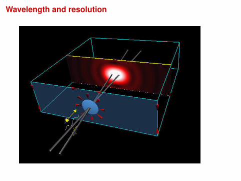
Resolution of Small Apertures

Two point sources far from the aperture each produce a diffrac-tion pattern.

If the angle subtended by the sources at the aperture is largeenough, the diffraction patterns are distinguishable as shownin Fig. (a).

If the angle is small, the diffraction patterns can overlap so thatthe sources are not well resolved as shown in Fig. (b).

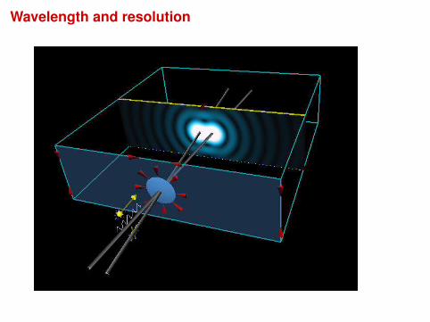
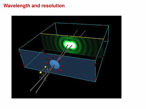
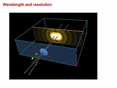
Wavelength and resolution

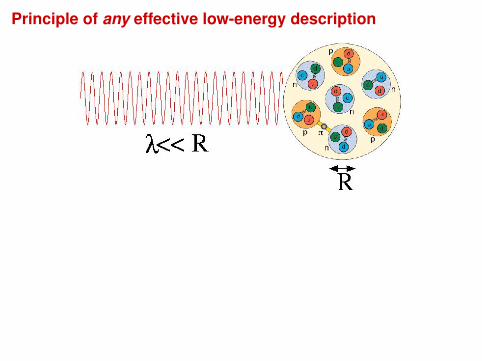
Principle of any effective low-energy description

If system is probed at low energies, fine details not resolved

Use low-energy variables for low-energy processesShort-distance structure can be replaced by somethingsimpler without distorting low-energy observables(cf. multipoles in classical electrodynamics)Could be a model or systematic (e.g., effective field theory)

Density in Pb⇔ low momentum⇔ low resolution (λ = h/p)but not so fast: the interaction can affect the resolution

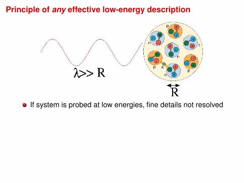
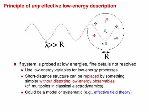
Principle of any effective low-energy description

If system is probed at low energies, fine details not resolvedUse low-energy variables for low-energy processesShort-distance structure can be replaced by somethingsimpler without distorting low-energy observables(cf. multipoles in classical electrodynamics)Could be a model or systematic (e.g., effective field theory)

Density in Pb⇔ low momentum⇔ low resolution (λ = h/p)but not so fast: the interaction can affect the resolution

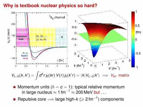
Why is textbook nuclear physics so hard?

VL=0(k , k ′) =

∫d3r j0(kr) V (r) j0(k ′r) = 〈k |VL=0|k ′〉 =⇒ Vkk ′ matrix

Momentum units (~ = c = 1): typical relative momentumin large nucleus ≈ 1 fm−1 ≈ 200 MeV but . . .

Repulsive core =⇒ large high-k (> 2 fm−1) components

Consequences of a repulsive core

0 2 4 6r [fm]

-0.1

0

0.1

0.2

0.3

0.4

|ψ(r)

|2 [fm

−3]

uncorrelatedcorrelated

0 2 4 6r [fm]

−100

0

100

200

300

400

V(r)

[MeV

]

0 2 4 6r [fm]

0

0.05

0.1

0.15

0.2

|ψ(r)

|2 [fm

−3]

Argonne v18

3S1 deuteron probability density

Probability at short separations suppressed =⇒ “correlations”

Short-distance structure⇔ high-momentum components

Greatly complicates expansion of many-body wave functions

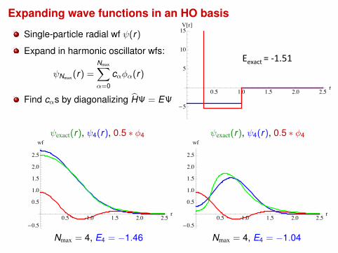
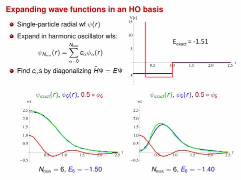
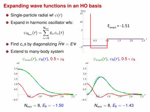
Expanding wave functions in an HO basis

Single-particle radial wf ψ(r)

Expand in harmonic oscillator wfs:

ψNmax (r) =

Nmax∑α=0

cαφα(r)

Find cαs by diagonalizing HΨ = EΨ

Extend to many-body system

Out[532]=

0.5 1.0 1.5 2.0 2.5r

-5

5

10

15V@rD

Eexact'=')1.51'

ψexact(r), ψ0(r), 0.5 ∗ φ0 ψexact(r), ψ0(r), 0.5 ∗ φ0

Out[476]=

0.5 1.0 1.5 2.0 2.5r

-0.5

0.5

1.0

1.5

2.0

2.5

wf

0.5 1.0 1.5 2.0 2.5r

-0.5

0.5

1.0

1.5

2.0

2.5

wf

Nmax = 0, E0 = −1.30 Nmax = 0, E0 = +5.23




ψNmax (r) =

Nmax∑α=0

cαφα(r)



Out[532]=

0.5 1.0 1.5 2.0 2.5r

-5

5

10

15V@rD

Eexact'=')1.51'


Out[480]=

0.5 1.0 1.5 2.0 2.5r

-0.5

0.5

1.0

1.5

2.0

2.5

wf

0.5 1.0 1.5 2.0 2.5r

-0.5

0.5

1.0

1.5

2.0

2.5

wf

Nmax = 2, E2 = −1.46 Nmax = 2, E2 = −0.87




ψNmax (r) =

Nmax∑α=0

cαφα(r)



Out[532]=

0.5 1.0 1.5 2.0 2.5r

-5

5

10

15V@rD

Eexact'=')1.51'


Out[485]=

0.5 1.0 1.5 2.0 2.5r

-0.5

0.5

1.0

1.5

2.0

2.5

wf

0.5 1.0 1.5 2.0 2.5r

-0.5

0.5

1.0

1.5

2.0

2.5

wf

Nmax = 4, E4 = −1.46 Nmax = 4, E4 = −1.04




ψNmax (r) =

Nmax∑α=0

cαφα(r)



Out[532]=

0.5 1.0 1.5 2.0 2.5r

-5

5

10

15V@rD

Eexact'=')1.51'


Out[489]=

0.5 1.0 1.5 2.0 2.5r

-0.5

0.5

1.0

1.5

2.0

2.5

wf

0.5 1.0 1.5 2.0 2.5r

-0.5

0.5

1.0

1.5

2.0

2.5

wf

Nmax = 6, E6 = −1.50 Nmax = 6, E6 = −1.40




ψNmax (r) =

Nmax∑α=0

cαφα(r)



Out[532]=

0.5 1.0 1.5 2.0 2.5r

-5

5

10

15V@rD

Eexact'=')1.51'


Out[493]=

0.5 1.0 1.5 2.0 2.5r

-0.5

0.5

1.0

1.5

2.0

2.5

wf

0.5 1.0 1.5 2.0 2.5r

-0.5

0.5

1.0

1.5

2.0

2.5

wf

Nmax = 8, E8 = −1.50 Nmax = 8, E8 = −1.43

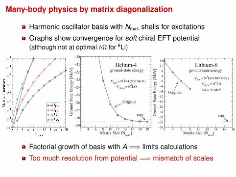
Many-body physics by matrix diagonalization

Harmonic oscillator basis with Nmax shells for excitations

Graphs show convergence for soft chiral EFT potential(although not at optimal ~Ω for 6Li)

2 4 6 8 10 12 14 16 18 20Matrix Size [N

max]

−29

−28

−27

−26

−25

−24

−23

−22

−21

−20

Gro

un

d S

tate

En

erg

y [

MeV

]

Original

expt.

VNN

= N3LO (500 MeV)

Helium-4

VNNN

= N2LO

ground-state energy

2 4 6 8 10 12 14 16 18

Matrix Size [Nmax

]

−36

−32

−28

−24

−20

−16

−12

−8

−4

0

4

8

12

16

Gro

un

d-S

tate

En

erg

y [

MeV

]

Lithium-6

expt.

Originalh- Ω = 20 MeV

ground-state energy

VNN

= N3LO (500 MeV)

VNNN

= N2LO

Factorial growth of basis with A =⇒ limits calculations

Too much resolution from potential =⇒ mismatch of scales

What if your theory has too much resolution?

What if your theory has too much resolution?

Claim: Nuclear physics with textbook V (r) is like using beer coasters!

Less painful to use a low-resolution version!

High resolution Low resolution

Can greatly reduce storage without distorting message

Resolution was lowered here by “block spinning”

Alternative: apply a low-pass filter

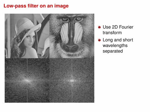
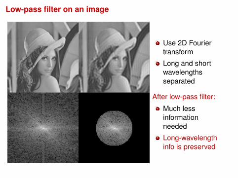
Low-pass filter on an image

Use 2D Fouriertransform

Long and shortwavelengthsseparated

After low-pass filter:

Much lessinformationneeded

Long-wavelengthinfo is preserved

Try a low-pass filter on nuclear V (r)

=⇒ Set to zero high momentum (k > 2 fm−1) matrix elementsand see the effect on low-energy observables

Use Phase Shifts to Test

0 R

sin(kr+δ)

r

0 100 200 300Elab (MeV)

−20

0

20

40

60

phas

e sh

ift (d

egre

es)

AV18

1S0

Here: 1S0 (spin-singlet, L = 0, J = 0) neutron-proton scattering

Different phase shifts in each partial wave channel

Effect of low-pass filter on observables

0 R

sin(kr+δ)

r

0 100 200 300E

lab (MeV)

−20

0

20

40

60

ph

ase

shif

t (d

egre

es)

1S

0

AV18 phase shifts

k = 2 fm−1

Effect of low-pass filter on observables

0 R

sin(kr+δ)

r

0 100 200 300E

lab (MeV)

−20

0

20

40

60

ph

ase

shif

t (d

egre

es)

1S

0

AV18 phase shifts

after low-pass filter

k = 2 fm−1

Why did our low-pass filter fail?

Basic problem: low k and high kare coupled (mismatched dof’s!)

E.g., perturbation theoryfor (tangent of) phase shift:

〈k |V |k〉+∑k ′

〈k |V |k ′〉〈k ′|V |k〉(k2 − k ′2)/m

+ · · ·

Solution: Unitary transformationof the H matrix =⇒ decouple!

En = 〈Ψn|H|Ψn〉 U†U = 1= (〈Ψn|U†)UHU†(U|Ψn〉)= 〈Ψn|H|Ψn〉

Here: Decouple using RG 0 100 200 300E

lab (MeV)

−20

0

20

40

60

phas

e sh

ift

(deg

rees

)

1S

0

AV18 phase shifts

after low-pass filter

k = 2 fm−1

Preview: Decoupling with the similarity RG

Preview: Consequences of a repulsive core revisited

0 2 4 6r [fm]

-0.1

0

0.1

0.2

0.3

0.4

|ψ(r)

|2 [fm

−3]


0 2 4 6r [fm]

−100

0

100

200

300

400

V(r)

[MeV

]

0 2 4 6r [fm]

0

0.05

0.1

0.15

0.2

0.25

|ψ(r)

|2 [fm

−3]

Argonne v18

3S1 deuteron probability density

Probability at short separations suppressed =⇒ “correlations”

Short-distance structure⇔ high-momentum components

Greatly complicates expansion of many-body wave functions


0 2 4 6r [fm]

-0.1

0

0.1

0.2

0.3

0.4

|ψ(r)

|2 [fm

−3]


0 2 4 6r [fm]

−100

0

100

200

300

400

V(r)

[MeV

]

0 2 4 6r [fm]

0

0.05

0.1

0.15

0.2

0.25

|ψ(r

)|2 [

fm−

3]

Argonne v18

λ = 4.0 fm-1

λ = 3.0 fm-1

λ = 2.0 fm-1

3S

1 deuteron probability density

softened

original

Transformed potential =⇒ no short-range correlations in wf!

Can it really be so different in the interior?


0 2 4 6

r [fm]

-0.1

0

0.1

0.2

0.3

0.4

r2|ψ

(r)|

2 [

fm−

1]


0 2 4 6

r [fm]

−100

0

100

200

300

400

V(r

) [M

eV

]

0 2 4 6r [fm]

0

0.05

0.1

0.15

0.2

0.25

0.3

0.35

r2|ψ

(r)|

2 [

fm−

1]

Argonne v18

λ = 4.0 fm-1

λ = 3.0 fm-1

λ = 2.0 fm-1

3S

1 deuteron probability density

Transformed potential =⇒ no short-range correlations in wf!

What part of the coordinate-space wave function is measurable?

What about the high-momentum tail in momentum space?

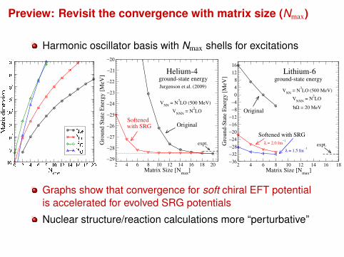
Preview: Revisit the convergence with matrix size (Nmax)


2 4 6 8 10 12 14 16 18 20Matrix Size [N

max]

−29

−28

−27

−26

−25

−24

−23

−22

−21

−20

Gro

un

d S

tate

En

erg

y [

MeV

]

Original

expt.

VNN

= N3LO (500 MeV)

Helium-4

VNNN

= N2LO

ground-state energy

2 4 6 8 10 12 14 16 18

Matrix Size [Nmax

]

−36

−32

−28

−24

−20

−16

−12

−8

−4

0

4

8

12

16

Gro

un

d-S

tate

En

erg

y [

MeV

]

Lithium-6

expt.


ground-state energy

VNN

= N3LO (500 MeV)

VNNN

= N2LO

Graphs show that convergence for soft chiral EFT potentialis accelerated for evolved SRG potentials

Nuclear structure/reaction calculations more “perturbative”

Preview: Revisit the convergence with matrix size (Nmax)


2 4 6 8 10 12 14 16 18 20Matrix Size [N

max]

−29

−28

−27

−26

−25

−24

−23

−22

−21

−20

Gro

un

d S

tate

En

erg

y [

MeV

]

Original

expt.

VNN

= N3LO (500 MeV)

Helium-4

Softenedwith SRG

VNNN

= N2LO

ground-state energy

Jurgenson et al. (2009)

2 4 6 8 10 12 14 16 18

Matrix Size [Nmax

]

−36

−32

−28

−24

−20

−16

−12

−8

−4

0

4

8

12

16

Gro

un

d-S

tate

En

erg

y [

MeV

]

Lithium-6

expt.


Softened with SRG

ground-state energy

VNN

= N3LO (500 MeV)

VNNN

= N2LO

λ = 1.5 fm−1

λ = 2.0 fm−1

Graphs show that convergence for soft chiral EFT potentialis accelerated for evolved SRG potentials

Nuclear structure/reaction calculations more “perturbative”

Applications of Renormalization Group Methods in Nuclear ...ntg/8805/slides/HUGS_2014_furn... ·...

Documents

Transcript of Applications of Renormalization Group Methods in Nuclear ...ntg/8805/slides/HUGS_2014_furn... ·...