Applications of non-linear algebra to biology

by

Dustin Alexander Cartwright

A dissertation submitted in partial satisfaction of the

requirements for the degree of

Doctor of Philosophy

in

Mathematics

and the Designated Emphasis

in

Computational and Genomic Biology

in the

Graduate Division

of the

University of California, Berkeley

Committee in charge:

Professor Bernd Sturmfels, ChairProfessor Lior PachterProfessor Yun S. Song

Fall 2010

Applications of non-linear algebra to biology

Copyright 2010by

Dustin Alexander Cartwright

1

Abstract

Applications of non-linear algebra to biology

by

Dustin Alexander Cartwright

Doctor of Philosophy in Mathematicsand the Designated Emphasis in Computational and Genomic Biology

University of California, Berkeley

Professor Bernd Sturmfels, Chair

We present two applications of non-linear algebra to biology. Our first application is to theanalysis of gene expression data from Arabidoposis roots. In Chapter 2, we present a methodfor computing non-negative roots to certain systems of polynomials. This algorithm is basedon a generalization of the Expectation-Maximization and Iterative Proportional Fitting fromstatistics. In Chapter 3, this method is applied to a model for gene expression coming fromroots of the Arabidopsis plant. Variation in gene expression is one method in which differenttissue types develop different functional characteristics. Our model for gene expression inthese roots is non-linear and so we apply the method from Chapter 2.

Our second application is the use of secant varieties to study mixture models for thedistribution of single-nucleotide polymorphisms in genes. In Chapter 4, we give generatorsfor the defining ideal of the first 5 secant varieties of P2 × Pn−1 embedded by O(1, 2). Ourequations come from a generalization of the flattening of a tensor, which we call an exteriorflattening. The study of secant varieties is a classical subject in algebraic geometry, whichhas recently been connected to applications in algebraic statistics. In Chapter 5, this con-nection is used in order to understand how single-nucleotide polymorphisms occur withinhuman genes. Because genes perform important functions, there is selective pressure againstmutations which affect the gene’s behavior. As we show, these selective pressures are closelytied to the nature by which genetic sequence codes for the constituent amino acids of aprotein.

i

Contents

List of Figures ii

List of Tables iii

1 Introduction 11.1 Algebraic statistics . . . . . . . . . . . . . . . . . . . . . . . . . . . . . . . . 21.2 Maximum likelihood estimation . . . . . . . . . . . . . . . . . . . . . . . . . 3

2 Non-negative solutions to positive systems of polynomial equations 52.1 Algorithm . . . . . . . . . . . . . . . . . . . . . . . . . . . . . . . . . . . . . 72.2 Proof of convergence . . . . . . . . . . . . . . . . . . . . . . . . . . . . . . . 102.3 Universality . . . . . . . . . . . . . . . . . . . . . . . . . . . . . . . . . . . . 15

3 Gene expression in Arabidopsis roots 183.1 Methods . . . . . . . . . . . . . . . . . . . . . . . . . . . . . . . . . . . . . . 213.2 Results . . . . . . . . . . . . . . . . . . . . . . . . . . . . . . . . . . . . . . . 283.3 Discussion . . . . . . . . . . . . . . . . . . . . . . . . . . . . . . . . . . . . . 32

4 Semi-symmetric tensor ranks 344.1 The κ-invariant of a 3-tensor . . . . . . . . . . . . . . . . . . . . . . . . . . . 364.2 The κ-invariant for partially symmetric 3-tensors . . . . . . . . . . . . . . . 434.3 Subspace varieties of partially symmetric tensors . . . . . . . . . . . . . . . . 494.4 Secant varieties of P2 × Pn−1 embedded by O(1, 2) . . . . . . . . . . . . . . . 51

5 How are SNPs distributed in genes? 565.1 Testing mixture models . . . . . . . . . . . . . . . . . . . . . . . . . . . . . . 565.2 The distribution of SNPs in human genes . . . . . . . . . . . . . . . . . . . . 59

Bibliography 64

ii

List of Figures

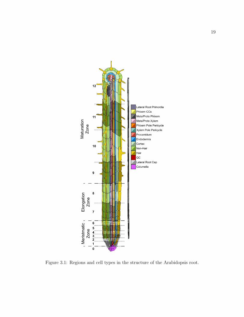
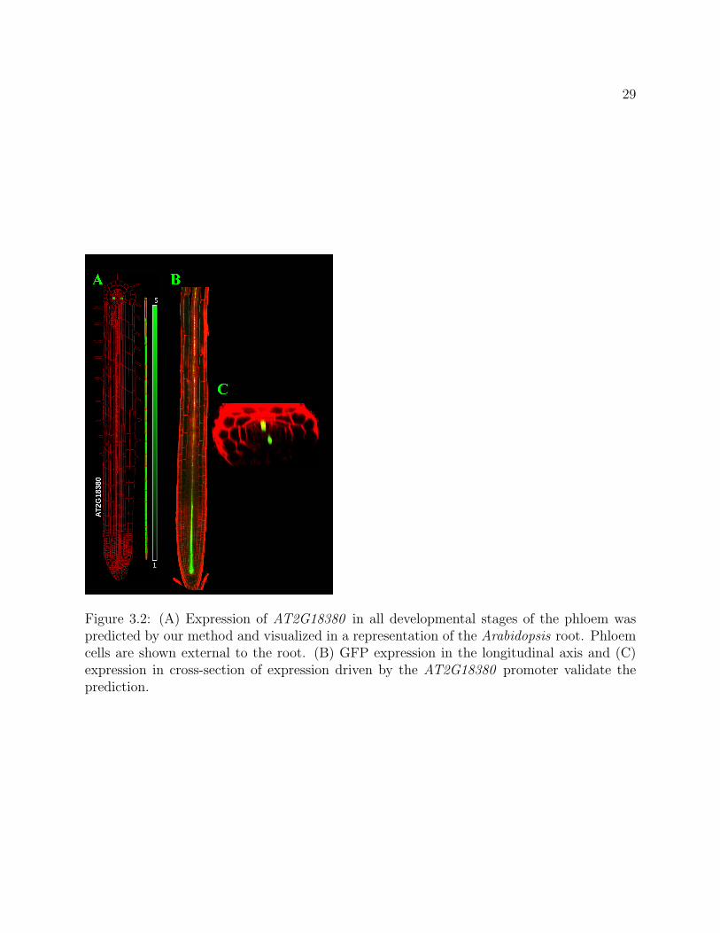
3.1 Regions and cell types in the structure of the Arabidopsis root. . . . . . . . . 193.2 (A) Expression of AT2G18380 in all developmental stages of the phloem was

predicted by our method and visualized in a representation of the Arabidopsisroot. Phloem cells are shown external to the root. (B) GFP expression in thelongitudinal axis and (C) expression in cross-section of expression driven bythe AT2G18380 promoter validate the prediction. . . . . . . . . . . . . . . . 29

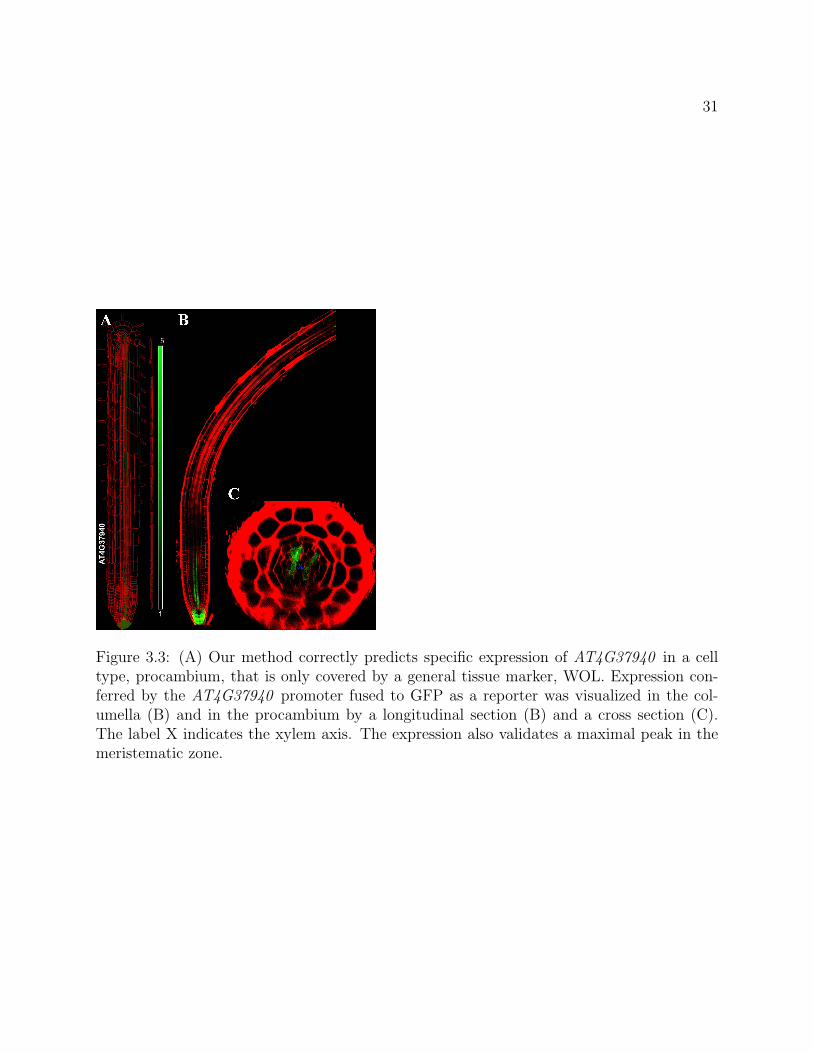
3.3 (A) Our method correctly predicts specific expression of AT4G37940 in acell type, procambium, that is only covered by a general tissue marker, WOL.Expression conferred by the AT4G37940 promoter fused to GFP as a reporterwas visualized in the columella (B) and in the procambium by a longitudinalsection (B) and a cross section (C). The label X indicates the xylem axis. Theexpression also validates a maximal peak in the meristematic zone. . . . . . 31

4.1 The Schur module decompositions of (Iκ1≤c1)c1+1 in the O(1, 1, 1) case whenk = m = n = 3. . . . . . . . . . . . . . . . . . . . . . . . . . . . . . . . . . . 42

iii

List of Tables

2.1 Eight iterations of the outer loop applied to the system of equations in (2.5). 8

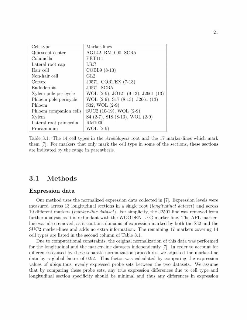
3.1 The 14 cell types in the Arabidopsis root and the 17 marker-lines which markthem [7]. For markers that only mark the cell type in some of the sections,these sections are indicated by the range in parenthesis. . . . . . . . . . . . . 21

3.2 The cell count matrix gives the number of cells in each spatiotemporal sub-region. The 13 rows correspond to longitudinal sections 1 through 13. Fromleft to right, the 14 columns correspond to the following spatiotemporal subre-gions: quiescent center, columella, lateral root cap, hair cell, non-hair cell, cor-tex, endodermis, xylem pole pericycle, phloem pole pericycle, phloem, phloemcompanion cells, xylem, lateral root primordia, and procambium. . . . . . . 23

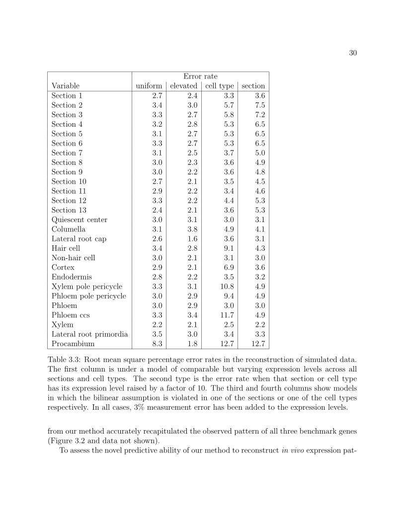
3.3 Root mean square percentage error rates in the reconstruction of simulateddata. The first column is under a model of comparable but varying expressionlevels across all sections and cell types. The second type is the error rate whenthat section or cell type has its expression level raised by a factor of 10. Thethird and fourth columns show models in which the bilinear assumption isviolated in one of the sections or one of the cell types respectively. In allcases, 3% measurement error has been added to the expression levels. . . . . 30

5.1 Occurrence of bases at HapMap loci. . . . . . . . . . . . . . . . . . . . . . . 595.2 Heterozygosity of HapMap loci by phase . . . . . . . . . . . . . . . . . . . . 595.3 Coding of bases by amino acid triplets. . . . . . . . . . . . . . . . . . . . . . 605.4 Haplotype base frequencies by phase in polymorphic sites from the HapMap

data. . . . . . . . . . . . . . . . . . . . . . . . . . . . . . . . . . . . . . . . . 605.5 Probabilities of obtaining a γ statistic at least as large as that of the contin-

gency table in Table 5.1. . . . . . . . . . . . . . . . . . . . . . . . . . . . . . 615.6 Categorization of amino acids based on number of codons which code for that

amino acid. . . . . . . . . . . . . . . . . . . . . . . . . . . . . . . . . . . . . 625.7 Resulting p-values for the δ statistic applied to SNP distributions in each of

the amino acid categories from Table 5.6. . . . . . . . . . . . . . . . . . . . . 62

iv

Acknowledgments

I’d like to acknowledge my mother, father, and sister for their support during my time ingraduate school. In addition, Philip Benfey, Siobhan Brady, Daniel Erman, Luke Oeding,and David Orlando were my co-authors on papers which served as a basis for this dissertation.I’d like to thank them for their collaboration on these papers and for the many things they’vetaught me. Lastly, I’d like to thank Bernd Sturmfels, for his tireless guidance, without whichthis document wouldn’t have been possible.

1

Chapter 1

Introduction

In this dissertation, we present two applications of non-linear algebra to biology. Our useof non-linear algebra includes both polynomial algebra, in which linear equations are replacedby polynomials, and multi-linear algebra, in which a single linear dependence, represented bya matrix, is replaced by multiple linear dependences, represented by a tensor. While linearalgebra is widely applied across many fields, the applications of non-linear algebra are not asprevalent. Non-linearity presents additional computational and interpretational challenges,some of which are addressed in this dissertation.

Because of the non-linearity, algebraic geometry becomes a key tool in our analysis.Algebraic geometry is the study of solutions to polynomial equations. Traditionally, thesolutions are taken to be in an algebraically closed field, such as the complex numbers, andthe strongest results still only hold in that context. For example, in Chapter 2, we study theproblem of finding only non-negative real solutions to polynomial equations. A number ofmethods exist for finding all complex solutions, from which the non-negative real solutionscan be selected. However, in cases when the number of complex solutions is vastly larger, itis more efficient to directly find just the non-negative real solutions, but few methods existin this situation. Our method for doing so is specifically built for real non-negative solutions.

Our first biological application is inferring expression patterns in Arabidoposis roots,which is presented in Chapter 3. Variation in gene expression level is a key factor in thedifferentiation of cell functionality, and thus essential to understanding the developmentalprocess. We describe a model for expression levels in the root of the Arabidopsis plant. Ourmodel is parametrized by bilinear polynomials. In order to solve these equations, we adaptthe methods of Expectation-Maximization and Iterative Proportional Fitting from statistics.These adaptations are described in Chapter 2.

In our second application, we look at the distribution of single-nucleotide polymorphisms(SNPs) in genes. Since genes code for proteins, whose functions are essential to the growthand reproduction of the organism in which they occur, there are selective pressures on themutations which can occur within a gene. In Chapter 5, we organize the occurrence of SNPswithin human genes into a 3 × 4 × 4 semi-symmetric contingency table. This contingency

2

table is tested against a mixture model with various numbers of hidden states in order tounderstand the interaction between phase within a codon and selective pressure. Our methodfor testing mixture models is based on having a determinantal representation for the secantvarieties of P2 × P3 embedded by the ample line bundle O(1, 2).

Chapter 4 is devoted to the secant varieties of P2 × Pn−1 embedded by O(1, 2). Inparticular, we give equations for the first 5 secant varieties of this Segre-Veronese variety,in a determinantal representation. This determinantal representation, together with the useof singular value decomposition, is what allows us to robustly test these conditions allowingthem to be the basis of a statistical test in Chapter 5.

1.1 Algebraic statistics

Algebraic statistics involves the application of algebraic geometry techniques to statisticalproblems [19]. We start with the definition of probabilistic model of an event on a discretestate space of n events as a function f : Ω → ∆n−1, where ∆n−1 is the (n − 1)-dimensionalsimplex, considered as the set of points in Rn

≥0 whose sum is 1, and Ω is a parameter space. Inalgebraic statistics, we define the function f by polynomials. Likewise, Ω is a semi-algebraicset in Rn, such as a product of simplices. One of the standard problems in algebraic statisticsis to find the ideal I of all polynomials vanishing on the image of f . One case of this problemis taken up in Chapter 4.

One application of knowing these equations is to provide a way to test whether a prob-ability distribution belongs to the image of the statistical model. Given data which comesfrom the model f , the counts of the different events can be normalized to give an empiricaldistribution which is close to being in the image of f . Consequently, the values polynomialsin I will be close to zero when evaluated at this point. However, the converse isn’t true:the set of probability distributions for which all polynomials in I vanish is, by definitionthe Zariski closure of the image of f , and the Zariski closure may be larger than the image.Over the complex numbers, the image of a polynomial map contains a dense open subsetof its Zariski closure, which is thus equal to the closure in the usual Euclidean topology.However, over the real numbers, the image of f may not be dense in its Zariski closure inthe Euclidean topology. In summary, the vanishing of the polynomials in I on a particulardistribution means that there exist complex parameters for which this distribution can beapproximated arbitrarily closely, but it may not be possible to choose these parameters tobe real.

Another difficulty with using the vanishing of polynomials to test membership in a sta-tistical model is the necessity of being robust to the presence of noise. The empirical dis-tribution calculated from a series of observations is unlikely to exactly reflect the actualprobability distribution. Therefore, using polynomial equations to test membership in astatistical model requires some way of doing it robustly. In Chapter 5, instead of using theequations of Theorem 4.4.3 directly, we leverage their origins as determinants and Pfaffians

3

of certain matrices. The robust estimation of the rank of a matrix can be performed usingsingular value decomposition, as will be described in Section 5.1. In essence, we have reduceda multi-linear problem to a linear one.

In Chapter 2, the need for robustness comes from a non-statistical model, but statisticalmethods are used to find an approximate solution. More specifically, we have a systemof real algebraic equations and we want to find parameters for which these equations areapproximately satisfied as closely as possible. Usual tools for solving polynomial equations,such as Grobner bases or numerical homotopies, work over the complex numbers. Whilethese methods have been developed to be numerically robust, they do not allow robustnessin the sense of relaxing equality constraints to approximate equality. Thus, in Chapter 2, wedevelop a method in polynomial algebra which builds on statistical techniques for maximumlikelihood estimation.

1.2 Maximum likelihood estimation

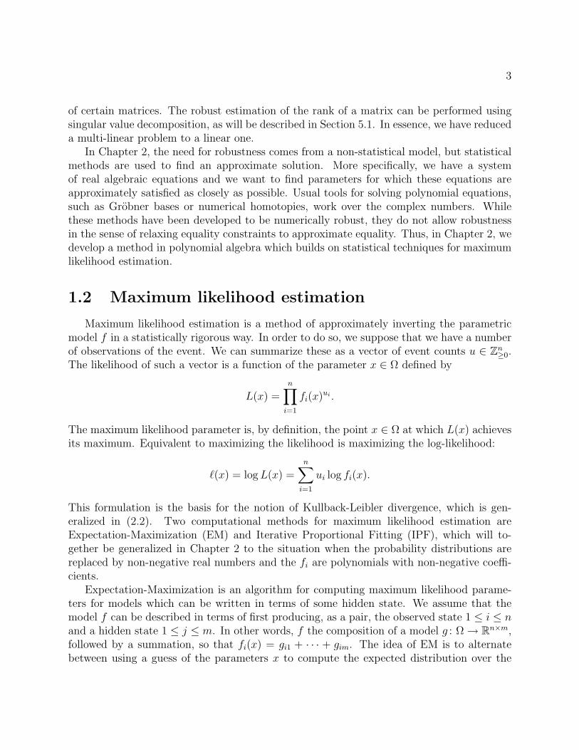
Maximum likelihood estimation is a method of approximately inverting the parametricmodel f in a statistically rigorous way. In order to do so, we suppose that we have a numberof observations of the event. We can summarize these as a vector of event counts u ∈ Zn

≥0.The likelihood of such a vector is a function of the parameter x ∈ Ω defined by

L(x) =n∏i=1

fi(x)ui .

The maximum likelihood parameter is, by definition, the point x ∈ Ω at which L(x) achievesits maximum. Equivalent to maximizing the likelihood is maximizing the log-likelihood:

`(x) = logL(x) =n∑i=1

ui log fi(x).

This formulation is the basis for the notion of Kullback-Leibler divergence, which is gen-eralized in (2.2). Two computational methods for maximum likelihood estimation areExpectation-Maximization (EM) and Iterative Proportional Fitting (IPF), which will to-gether be generalized in Chapter 2 to the situation when the probability distributions arereplaced by non-negative real numbers and the fi are polynomials with non-negative coeffi-cients.

Expectation-Maximization is an algorithm for computing maximum likelihood parame-ters for models which can be written in terms of some hidden state. We assume that themodel f can be described in terms of first producing, as a pair, the observed state 1 ≤ i ≤ nand a hidden state 1 ≤ j ≤ m. In other words, f the composition of a model g : Ω→ Rn×m,followed by a summation, so that fi(x) = gi1 + · · · + gim. The idea of EM is to alternatebetween using a guess of the parameters x to compute the expected distribution over the

4

hidden states (the E step), and using this distribution to compute the maximum likelihoodparameters for the hidden model (the M step). Thus, the M step requires a method forsolving the maximum likelihood problem for the hidden model. This algorithm is explicitlyspelled out in Section 2.1, where IPF is used for the M step. The EM algorithm is alsoapplied in Section 5.1, in which the hidden model is an independence model, and likelihoodmaximization can be trivially done in closed form. Note that EM is essentially a local search,it will converge to a local maximum, but not necessarily a global maximum.

Iterative Proportional Fitting finds maximum likelihood parameters for toric statisticalmodels, also called log-linear models. These are where the probabilities fi(x) are productsof powers of the parameters, i.e. fi(x) = xα1

1 · · ·xαkk . Thus, the logarithm of the probability

is linear in the logarithms of the parameters, explaining the name “log-linear.” As its nameimplies, IPF is an iterative algorithm for finding maximum likelihood parameters for such amodel. Note that a toric model is guaranteed to have a unique maximum likelihood solution,to which IPF will always converge [45, Thm. 1.10].

5

Chapter 2

Non-negative solutions to positivesystems of polynomial equations

This chapter is based on the paper “An algorithm for finding positive solutions to poly-nomial equations” [10]. We present an iterative numerical method for finding non-negativesolutions and approximate solutions to systems of polynomial equations. We require twoassumptions about our system of equations. First, for each equation, all the coefficientsother than the constant term must be non-negative. Second, there is a technical assumptionon the exponents, described at the beginning of Section 2.1, which, for example, is satisfiedif all non-constant terms have the same total degree. In Section 2.3, there is a discussion ofthe range of possible systems which can arise under these hypotheses.

Because of the assumption on signs, we can write our system of equations as∑α∈S

aiαxα = bi for i = 1, . . . , `, (2.1)

where the coefficients aiα are non-negative and the bi are positive, and S ⊂ Rn≥0 is a finite

set of possibly non-integer multi-indices. Our algorithm works by iteratively decreasing thegeneralized Kullback-Leibler divergence of the left-hand side and right-hand side of (2.1).The generalized Kullback-Leibler divergence of two positive vectors a and b is defined to be

D (a ‖b) :=∑i

(ai log

(aibi

)− ai + bi

). (2.2)

The standard Kullback-Leibler consists only of the first term and is defined only for proba-bility distributions, i.e. when the sum of each vector is 1. The last two terms are necessaryso that the generalized divergence has, for arbitrary positive vectors a and b, the propertyof being non-negative and zero exactly when a and b are equal (Proposition 2.1.4).

Our algorithm converges to local minima of the Kullback-Leibler divergence, includingexact solutions to the system (2.1). We will refer to local minima which are not exact

6

solutions as a approximate solutions, because in these cases, the equations (2.1) hold onlyapproximately. In order to find multiple local minima, we can repeat the algorithm forrandomly chosen starting points. For finding approximate solutions, this may be sufficient.However, there are no guarantees of completeness for the exact solutions obtained in thisway. Nonetheless, we hope that in certain situations, our algorithm will find applicationsboth for finding exact and approximate solutions.

Lee and Seung applied the EM algorithm to the problem of non-negative matrix factor-ization [38]. They introduced the generalized Kullback-Leibler divergence in (2.2) and usedit to find approximate non-negative matrix factorizations. Since the product of two matricescan be expressed by polynomials in the entries of the matrices, matrix-factorization is aspecial case of the equations in (2.1).

For finding exact solutions to arbitrary systems of polynomials, there are a variety ofapproaches which find all complex or all real solutions. Homotopy continuation methods findall complex roots of a system of equations [51]. Even to find only positive roots, these twomethods finds all complex or all real solutions, respectively. Lasserre, Laurent, and Rostalskihave applied semidefinite programming to find all real solutions to a system of equations and aslight modification of their algorithm will find all positive real solutions [36, 37]. Nonetheless,neither of these methods has any notion of approximate solutions.

For directly finding only positive real solutions, Bates and Sottile have proposed analgorithm based on fewnomials bounds on the number of real solutions [2]. However, theirmethod is only effective when the number of monomials (the set S in our notation) is slightlymore than the number of variables. Our method only makes weak assumptions on the set ofmonomials, but stronger assumptions on the coefficients.

Our inspiration comes from tools for maximum likelihood estimation in statistics. Param-eters which maximize the likelihood are exactly the parameters such that the model proba-bilities are closest to the empirical probabilities, in the sense of minimizing Kullback-Leiblerdivergence. Expectation-Maximization [45, Sec. 1.3] and Iterative Proportional Fitting [17]are well-known iterative methods for maximum likelihood estimation. We re-interpret thesealgorithms in the somewhat more general setting of finding approximate solutions to poly-nomial equations.

The impetus behind the work in this chapter was the need to find approximate positivesolutions to systems of bilinear equations which will appear in Chapter 3. In that applicationthe variables will represent expression levels, which only made sense as positive parameters.Moreover, in order to accommodate noise in the data, there are more equations than vari-ables, so it is necessary to find approximate solutions. Thus, the algorithm described in thischapter incorporates both the positivity and the robustness.

An implementation of our algorithm in the C programming language is freely availableat http://math.berkeley.edu/~dustin/pos/.

In Section 2.1, we describe the algorithm and the connection to maximum likelihoodestimation. In Section 2.2, we prove the necessary convergence for our algorithm. Finally,in Section 2.3, we show that even with our restrictions on the form of the equations, there

7

can be exponentially many positive real solutions.

2.1 Algorithm

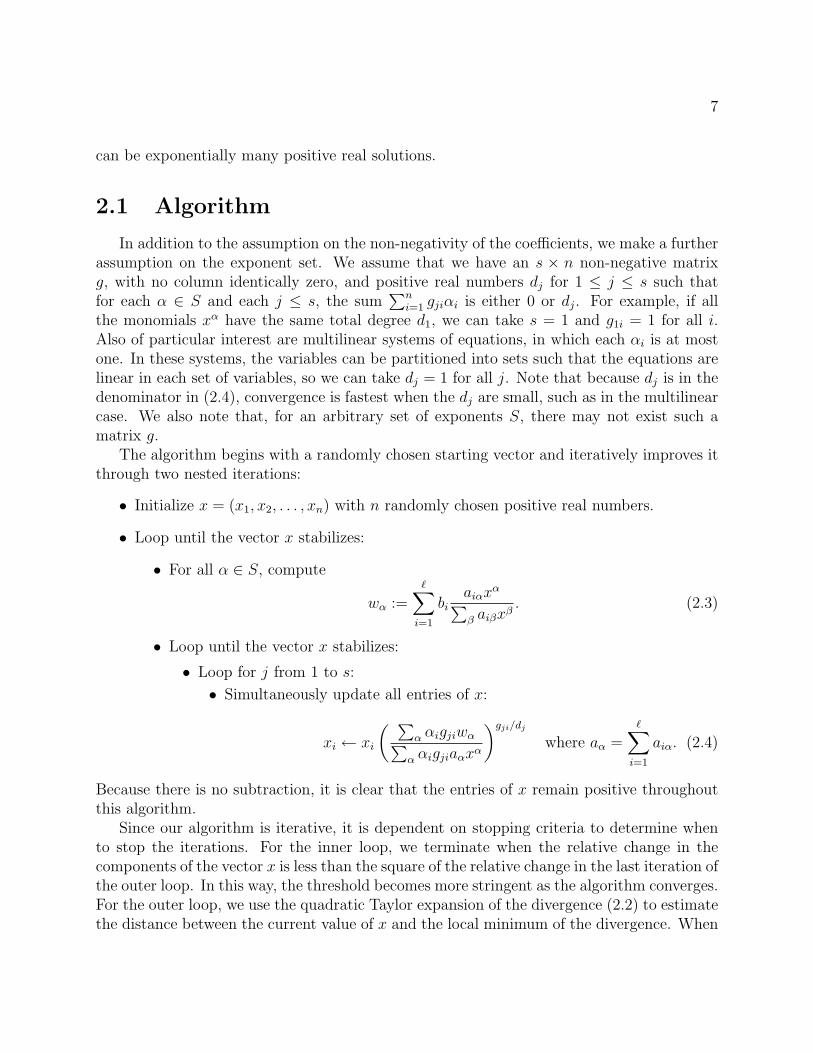
In addition to the assumption on the non-negativity of the coefficients, we make a furtherassumption on the exponent set. We assume that we have an s × n non-negative matrixg, with no column identically zero, and positive real numbers dj for 1 ≤ j ≤ s such thatfor each α ∈ S and each j ≤ s, the sum

∑ni=1 gjiαi is either 0 or dj. For example, if all

the monomials xα have the same total degree d1, we can take s = 1 and g1i = 1 for all i.Also of particular interest are multilinear systems of equations, in which each αi is at mostone. In these systems, the variables can be partitioned into sets such that the equations arelinear in each set of variables, so we can take dj = 1 for all j. Note that because dj is in thedenominator in (2.4), convergence is fastest when the dj are small, such as in the multilinearcase. We also note that, for an arbitrary set of exponents S, there may not exist such amatrix g.

The algorithm begins with a randomly chosen starting vector and iteratively improves itthrough two nested iterations:

• Initialize x = (x1, x2, . . . , xn) with n randomly chosen positive real numbers.

• Loop until the vector x stabilizes:

• For all α ∈ S, compute

wα :=∑i=1

biaiαx

α∑β aiβx

β. (2.3)

• Loop until the vector x stabilizes:

• Loop for j from 1 to s:

• Simultaneously update all entries of x:

xi ← xi

( ∑α αigjiwα∑α αigjiaαx

α

)gji/djwhere aα =

∑i=1

aiα. (2.4)

Because there is no subtraction, it is clear that the entries of x remain positive throughoutthis algorithm.

Since our algorithm is iterative, it is dependent on stopping criteria to determine whento stop the iterations. For the inner loop, we terminate when the relative change in thecomponents of the vector x is less than the square of the relative change in the last iteration ofthe outer loop. In this way, the threshold becomes more stringent as the algorithm converges.For the outer loop, we use the quadratic Taylor expansion of the divergence (2.2) to estimatethe distance between the current value of x and the local minimum of the divergence. When

8

Inner loop iterations x y5 0.6944381615 0.93274352544 0.6339861529 0.98628799823 0.6217014340 0.99686243695 0.6187745905 0.99936726676 0.6181817273 0.99987380898 0.6180632943 0.99997496989 0.6180397990 0.9999950375

11 0.6180351404 0.9999990163

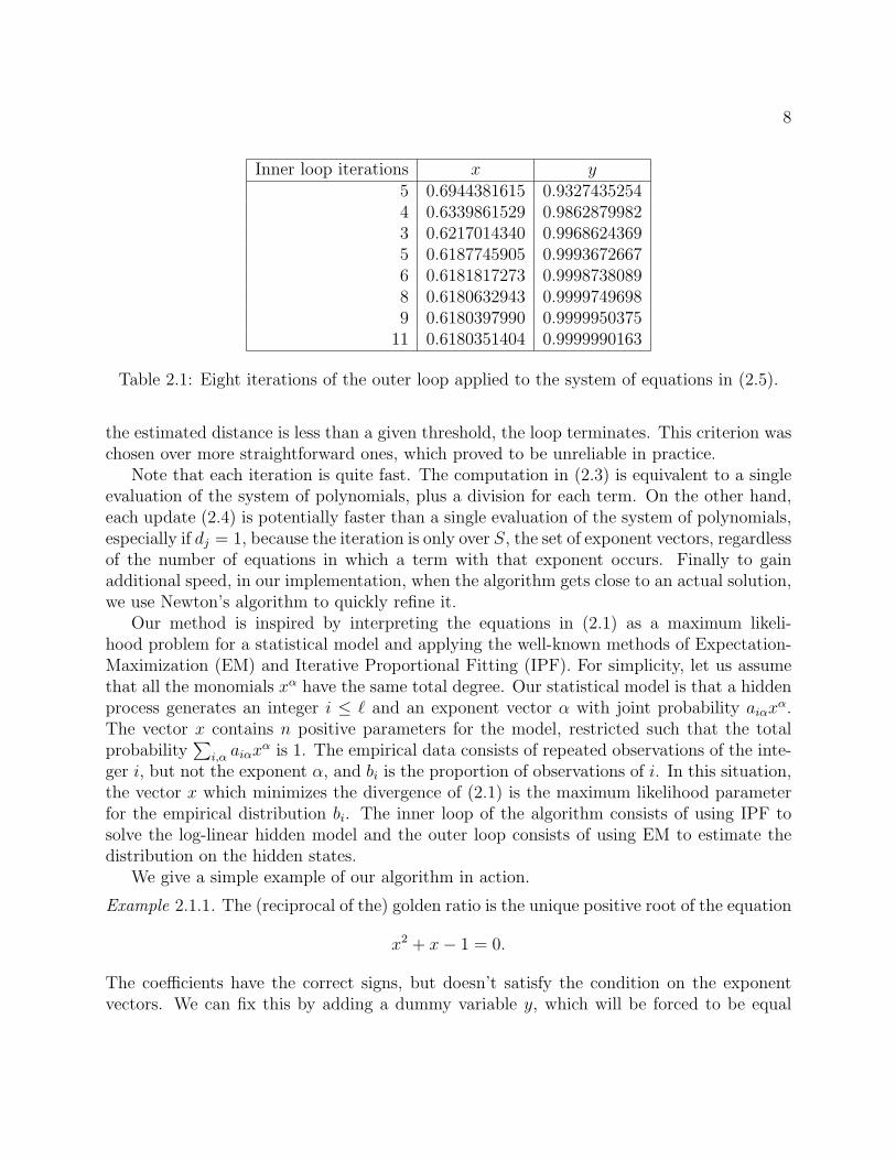
Table 2.1: Eight iterations of the outer loop applied to the system of equations in (2.5).

the estimated distance is less than a given threshold, the loop terminates. This criterion waschosen over more straightforward ones, which proved to be unreliable in practice.

Note that each iteration is quite fast. The computation in (2.3) is equivalent to a singleevaluation of the system of polynomials, plus a division for each term. On the other hand,each update (2.4) is potentially faster than a single evaluation of the system of polynomials,especially if dj = 1, because the iteration is only over S, the set of exponent vectors, regardlessof the number of equations in which a term with that exponent occurs. Finally to gainadditional speed, in our implementation, when the algorithm gets close to an actual solution,we use Newton’s algorithm to quickly refine it.

Our method is inspired by interpreting the equations in (2.1) as a maximum likeli-hood problem for a statistical model and applying the well-known methods of Expectation-Maximization (EM) and Iterative Proportional Fitting (IPF). For simplicity, let us assumethat all the monomials xα have the same total degree. Our statistical model is that a hiddenprocess generates an integer i ≤ ` and an exponent vector α with joint probability aiαx

α.The vector x contains n positive parameters for the model, restricted such that the totalprobability

∑i,α aiαx

α is 1. The empirical data consists of repeated observations of the inte-ger i, but not the exponent α, and bi is the proportion of observations of i. In this situation,the vector x which minimizes the divergence of (2.1) is the maximum likelihood parameterfor the empirical distribution bi. The inner loop of the algorithm consists of using IPF tosolve the log-linear hidden model and the outer loop consists of using EM to estimate thedistribution on the hidden states.

We give a simple example of our algorithm in action.

Example 2.1.1. The (reciprocal of the) golden ratio is the unique positive root of the equation

x2 + x− 1 = 0.

The coefficients have the correct signs, but doesn’t satisfy the condition on the exponentvectors. We can fix this by adding a dummy variable y, which will be forced to be equal

9

to 1:

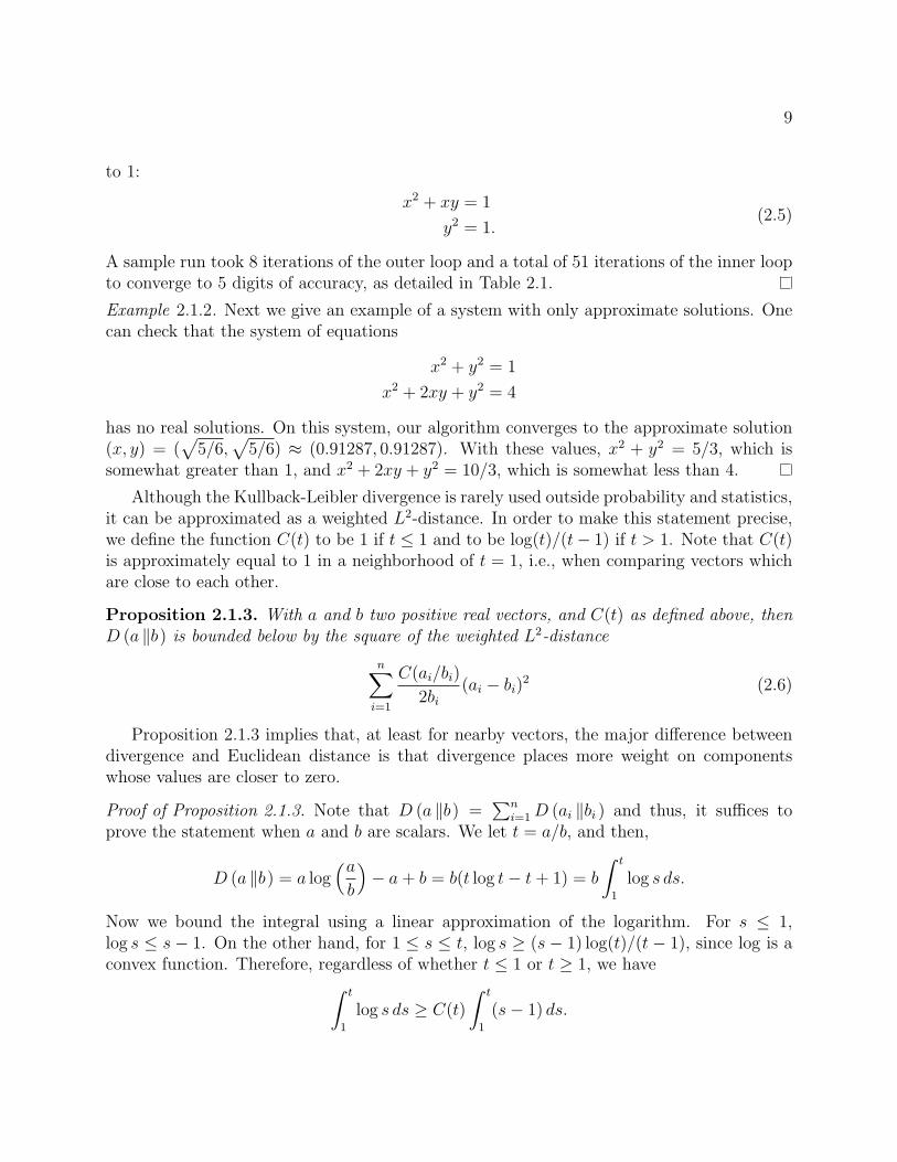
x2 + xy = 1

y2 = 1.(2.5)

A sample run took 8 iterations of the outer loop and a total of 51 iterations of the inner loopto converge to 5 digits of accuracy, as detailed in Table 2.1.

Example 2.1.2. Next we give an example of a system with only approximate solutions. Onecan check that the system of equations

x2 + y2 = 1

x2 + 2xy + y2 = 4

has no real solutions. On this system, our algorithm converges to the approximate solution(x, y) = (

√5/6,

√5/6) ≈ (0.91287, 0.91287). With these values, x2 + y2 = 5/3, which is

somewhat greater than 1, and x2 + 2xy + y2 = 10/3, which is somewhat less than 4.

Although the Kullback-Leibler divergence is rarely used outside probability and statistics,it can be approximated as a weighted L2-distance. In order to make this statement precise,we define the function C(t) to be 1 if t ≤ 1 and to be log(t)/(t− 1) if t > 1. Note that C(t)is approximately equal to 1 in a neighborhood of t = 1, i.e., when comparing vectors whichare close to each other.

Proposition 2.1.3. With a and b two positive real vectors, and C(t) as defined above, thenD (a ‖b) is bounded below by the square of the weighted L2-distance

n∑i=1

C(ai/bi)

2bi(ai − bi)2 (2.6)

Proposition 2.1.3 implies that, at least for nearby vectors, the major difference betweendivergence and Euclidean distance is that divergence places more weight on componentswhose values are closer to zero.

Proof of Proposition 2.1.3. Note that D (a ‖b) =∑n

i=1D (ai ‖bi ) and thus, it suffices toprove the statement when a and b are scalars. We let t = a/b, and then,

D (a ‖b) = a log(ab

)− a+ b = b(t log t− t+ 1) = b

∫ t

1

log s ds.

Now we bound the integral using a linear approximation of the logarithm. For s ≤ 1,log s ≤ s− 1. On the other hand, for 1 ≤ s ≤ t, log s ≥ (s− 1) log(t)/(t− 1), since log is aconvex function. Therefore, regardless of whether t ≤ 1 or t ≥ 1, we have∫ t

1

log s ds ≥ C(t)

∫ t

1

(s− 1) ds.

10

Combining this inequality with (2.1),

D (a ‖b) ≥ C(t)b

∫ t

1

(s− 1) ds =C(a/b)b

2

(ab− 1)2

=C(a/b)

2b(a− b)2,

which is the desired result.

As a corollary, we get:

Proposition 2.1.4. For vectors a and b of positive real numbers, the divergence D (a ‖b) isalways non-negative with D (a ‖b) = 0 if and only if a = b.

Proof. Since the quantity C(ai/bi) from Proposition 2.1.3 is always positive, each term ofthe summation in (2.6) is non-negative and it is zero if and only ai = bi.

2.2 Proof of convergence

In this section we prove our main theorem:

Theorem 2.2.1. The Kullback-Leibler divergence

∑i=1

D

(bi

∥∥∥∥∥∑α∈S

aiαxα

). (2.7)

is weakly decreasing during the algorithm in Section 2.1. Moreover, assuming that the set Scontains a multiple of each unit vector ei, i.e. some power of each xi appears in the system ofequations, then the vector x converges to a critical point of the function (2.7) or the boundaryof the positive orthant.

Remark 2.2.2. The condition that S contains a pure power of each variable xi is in orderto ensure that the vector x remains bounded during the algorithm.

We begin by establishing several basic properties of the generalized Kullback-Leibler di-vergence in Lemmas 2.2.3 and 2.2.4. The proof of Theorem 2.2.1 itself is divided into twoparts, corresponding to the two nested iterative loops. The first step is to prove that the up-dates (2.4) in the inner loop converge a local minimum of the divergence D (wα ‖aαxα ). Thesecond step is to show that this implies that the outer loop strictly decreases the divergencefunction (2.7), with equality only at a critical point.

Lemma 2.2.3. Suppose that a and b are vectors of n positive real numbers. Let t be anypositive real number, and then

D (a ‖tb) = D (a ‖b) + (t− 1)m∑i=1

bi −m∑i=1

ai log t

11

Proof. As in the proof of Proposition 2.1.3, we can assume that a and b are scalars. In thiscase, it becomes a straightforward computation.

Lemma 2.2.4. If a and b are vectors of m positive real numbers, then we can relate theirdivergence to the divergence of their sums by

D (a ‖b) = D (∑m

i=1 ai ‖∑m

i=1 bi ) +D

(a

∥∥∥∥∑mi=1 ai∑mi=1 bi

b

).

Proof. We let A =∑m

i=1 ai and B =∑m

i=1 bi, and apply Lemma 2.2.3 to the last term:

D

(a

∥∥∥∥ABb)

= D (a ‖b) +

(A

B− 1

)B − A log

A

B

= D (a ‖b)− A logA

B+ A−B = D (a ‖b)−D (A ‖B ) .

After rearranging, we get the desired expression.

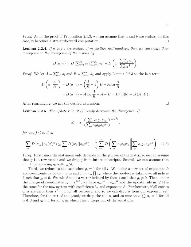
Lemma 2.2.5. The update rule (2.4) weakly decreases the divergence. If

x′i = xi

( ∑α αigjiwα∑α αigjiaαx

α

)gji/dj,

for any j ≤ s, then

∑α

D (wα ‖aα(x′)α ) ≤∑α

D (wα ‖aαxα )− 1

dj

n∑i=1

D

(∑α

αigjiwα

∥∥∥∥∥∑α

αigjiaαxα

). (2.8)

Proof. First, since the statement only depends on the jth row of the matrix g, we can assumethat g is a row vector and we drop j from future subscripts. Second, we can assume thatd = 1 by replacing gi with gi/d.

Third, we reduce to the case when gi = 1 for all i. We define a new set of exponents αand coefficients aα by αi = giαi and aα = aα

∏xi, where the product is taken over all indices

i such that gi = 0. We take x to be a vector indexed by those i such that gi 6= 0. Then, underthe change of coordinates xi = x

1/gii , we have aαx

α = aαxα and the update rule in (2.4) is

the same for the new system with coefficients aα and exponents α. Furthermore, if all entriesof α are zero, then xα = 1 for all vectors x and so we can drop α from our exponent set.Therefore, for the rest of the proof, we drop the tildes, and assume that

∑i αi = 1 for all

α ∈ S and gi = 1 for all i, in which case g drops out of the equations.

12

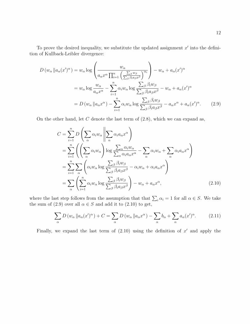
To prove the desired inequality, we substitute the updated assignment x′ into the defini-tion of Kullback-Leibler divergence:

D (wα ‖aα(x′)α ) = wα log

wα

aαxα∏n

i=1

( Pβ wβP

β βiaβxβ

)αi− wα + aα(x′)α

= wα logwαaαxα

−n∑i=1

αiwα log

∑β βiwβ∑β βiaβx

β− wα + aα(x′)α

= D (wα ‖aαxα )−n∑i=1

αiwα log

∑β βiwβ∑β βiaβx

β− aαxα + aα(x′)α. (2.9)

On the other hand, let C denote the last term of (2.8), which we can expand as,

C =n∑i=1

D

(∑α

αiwα

∥∥∥∥∥∑α

αiaαxα

)

=n∑i=1

((∑α

αiwα

)log

∑α αiwα∑α αiaαx

α−∑α

αiwα +∑α

αiaαxα

)

=n∑i=1

∑α

(αiwα log

∑β βiwβ∑β βiaβx

β− αiwα + αiaαx

α

)

=∑α

(n∑i=1

αiwα log

∑β βiwβ∑β βiaβx

β

)− wα + aαx

α, (2.10)

where the last step follows from the assumption that that∑

i αi = 1 for all α ∈ S. We takethe sum of (2.9) over all α ∈ S and add it to (2.10) to get,∑

α

D (wα ‖aα(x′)α ) + C =∑α

D (wα ‖aαxα )−∑α

bα +∑α

aα(x′)α. (2.11)

Finally, we expand the last term of (2.10) using the definition of x′ and apply the

13

arithmetic-geometric mean inequality,∑α

aα(x′)α =∑α

aαxα

n∏i=1

( ∑β βibβ∑

β βiaβxβ

)αi

≤∑α

aαxα

n∑i=1

αi

∑β βibβ∑

β βiaβxβ

=n∑i=1

(∑α

αiaαxα

) ∑β βibβ∑

β βiaβxβ

=n∑i=1

∑β

βibβ =∑β

bβ.

Together with (2.11), this gives the desired inequality.

Proposition 2.2.6. A positive vector x is a fixed point of the update rule (2.4) for all1 ≤ j ≤ s if and only if x is a critical point of the divergence function

∑αD (wα ‖aαxα ).

Proof. For the update rule to be constant means that the numerator and denominator in(2.4) are equal, i.e. ∑

α

αigjiaαxα =

∑α

αigjiwα for all i and j. (2.12)

By our assumption on g, for each i, some gji is non-zero, so (2.12) is equivalent to∑α

αiaαxα =

∑α

αiwα for all i. (2.13)

On the other hand, we compute the partial derivative

∂

∂xi

∑α

D (wα ‖aαxα ) =∑α

−wααixi

+ αiaαxα

xi.

Since each xi is assumed to be non-zero, it is clear that all partial derivatives being zero isequivalent to (2.13).

Lemma 2.2.7. If we define wα as in (2.3), then

n∑i=1

D

(bi

∥∥∥∥∥∑α

aiα(x′)α

)−

n∑i=1

D

(bi

∥∥∥∥∥∑α

aiαxα

)≤∑α

D (wα ‖aα(x′)α )−∑α

D (wα ‖aαxα ) .

Moreover, a positive vector x is a fixed point of the update rule if and only if x is a criticalpoint for the divergence function.

14

Proof. We consider ∑i,α

D (wiα ‖aiα(x′)α ) where wiα =biaiαx

α∑β aiβx

β, (2.14)

and apply Lemma 2.2.4 in two different ways. First, by applying Lemma 2.2.4 to each groupof (2.14) with fixed α, we get

∑i,α

D (wiα ‖aiα(x′)α ) =∑α

D (wα ‖aα(x′)α ) +∑i,α

D

(wiα

∥∥∥∥∥∑

j wjα∑j aα(x′)α

aiα(x′)α

).

In the last term, the monomials (x′)α cancel and so it is a constant independent of x′ whichwe denote E. On the other hand, we can apply Lemma 2.2.4 to each group in (2.14) withfixed i,

∑i,α

D (wiα ‖aiα(x′)α ) =∑i

D

(bi

∥∥∥∥∥∑α

aiα(x′)α

)+∑i,α

D

(wiα

∥∥∥∥∥ biaiα(x′)α∑β aiβ(x′)β

).

We can combine these equations to get

∑i

D

(bi

∥∥∥∥∥∑α

aiα(x′)α

)=∑α

D (wiα ‖aα(x′)α ) +E−∑i,α

D

(wiα

∥∥∥∥∥ biaiα(x′)α∑β aiβ(x′)β

). (2.15)

By Proposition 2.1.4, the last term of (2.15) is non-negative, and by the definition of wiα, itis zero for x′ = x. Therefore, any value of x′ which decreases the first term compared to xwill also decrease the left hand side by at least as much, which is the desired inequality.

In order to prove the statement about the derivative, we consider the derivative of (2.15)at x′ = x. Because the last term is minimized at x′ = x, its derivative is zero, so

∂

∂x′j

∣∣∣∣x′=x

∑i

D

(bi

∥∥∥∥∥∑α

aiα(x′)α

)=

∂

∂x′j

∣∣∣∣x′=x

∑i,α

D (wiα ‖aiα(x′)α ) .

By Proposition 2.2.6, a positive vector x is a fixed point of the inner loop if and only if thesepartial derivatives on the right are zero for all indices j, which is the definition of a criticalpoint.

Proof of Theorem 2.2.1. The Kullback-Leibler divergence∑

αD (wα ‖aαxα ) decreases at eachstep of the inner loop by Lemma 2.2.5. Thus, by Lemma 2.2.7, the divergence

n∑i=1

D

(bi

∥∥∥∥∥∑α

aiαxα

)(2.16)

15

decreases at least as much. However, the divergence (2.16) is non-negative according toProposition 2.1.4. Therefore, the magnitude of the decreases in divergence must approachzero over the course of the algorithm. By Lemma 2.2.5, this means that the quantity C inthat theorem must approach zero. By Proposition 2.1.4, this means that the quantities inthat divergence approach each other. However, up to a power, these are the numerator anddenominator of the factor in the update rule (2.4), so the difference between consecutivevectors x approaches zero.

Thus, we just need to show that x remains bounded. However, since some power of eachvariable xi occurs in some equation, as xi gets large, the divergence for that equation alsogets arbitrarily large. Therefore, each xi must remain bounded, so the vector x must have alimit as the algorithm is iterated. If this limit is in the interior of the positive orthant, thenit must be a fixed point. By Lemma 2.2.7 and Proposition 2.2.6, this fixed point must be acritical point of the divergence (2.7).

2.3 Universality

Although the restriction on the exponents and especially the positivity of the coefficientsseem like strong conditions, such systems can nonetheless be quite complex. In this section,we investigate the breadth of such equations.

Proposition 2.3.1. For any system of ` real polynomial equations in n variables, thereexists a system of ` + 1 polynomial equations in n + 1 variables, in the form (2.1), suchthat the positive solutions (x1, . . . , xn) to the former system are in bijection with the positivesolutions (x′1, . . . , x

′n+1) of the latter, with x′i = xi/xn+1.

Proof. We write our system of equations as∑

α∈S aiαxα = 0 for 1 ≤ i ≤ `, where S ⊂ Nn

is an arbitrary finite set of exponents and aiα are any real numbers. We let d be themaximum degree of any monomial xα for α ∈ S. We homogenize the equations with a newvariable xn+1. Explicitly, define S ′ ⊂ Nn+1 to consist of α′ = (α, d−

∑i αi) for all α in S and

we also set aiα′ = aiα. We add a new equation with coefficients a`+1,α = 1 for all α ∈ S ′ andb`+1 = 1. For this system, we can clearly take g1i = 1 and d1 = d to satisfy the conditionon exponents. Furthermore, for any positive solution (x1, . . . , xn) to the original system of

equations, (x′1, . . . , x′n+1) with x′i = xi/

(∑α x

α)1/d

and x′n+1 = 1/(∑

α xα)1/d

is a solutionto the homogenized system of equations.

Next, we add a multiple of the last equation to each of the others in order to makeall the coefficients positive. For each 1 ≤ i ≤ `, choose a positive bi > −minαaiα |α ∈ S ′, and define a′iα = aiα + bi. By construction, the resulting system has all positivecoefficients, and since the equations are formed from the previous equations by elementarylinear transformations, the set of solutions are the same.

The practical use of the construction in the proof of Proposition 2.3.1 is mixed. The firststep, of homogenizing to deal with arbitrary sets of exponents, is a straightforward way of

16

guaranteeing the existence of the matrix g. However, for large systems, the second step tendsto produce an ill-conditioned coefficient matrix. In these cases, our algorithm converges veryslowly. Nonetheless, Proposition 2.3.1 shows that, in the worst case, systems satisfying ourhypotheses can be as complicated as arbitrary polynomial systems.

Proposition 2.3.2. There exist bilinear equations in 2m variables with(2m−2m−1

)positive real

solutions.

Proof. We use a variation on the technique used to prove Proposition 2.3.1.First, we pick 2m− 2 generic homogeneous linear functions b1, . . . , b2m−2 on m variables.

By generic, we mean for any m of the bk, the only simultaneous solution of all m linearequations is the trivial one. This genericity implies that any m− 1 of the bk define a pointin Pm−1 By taking a linear changes of coordinates in each set of variables, we can assumethat all of these points are positive, i.e. have a representative consisting of all positive realnumbers.

Then we consider the system of equations

bk(x1, . . . , xm) · bk(xm+1, . . . , xn) = 0, for 1 ≤ k ≤ 2m− 2 (2.17)

(x1 + . . .+ xm)(xm+1 + . . .+ x2m) = 1 (2.18)

x1 + . . .+ xm = 1. (2.19)

The equations (2.17) are bihomogeneous and so we can think of their solutions in Pm−1 ×Pm−1. There are exactly

(2m−2m−1

)positive real solutions, corresponding to the subsets A ⊂

[2m − 2] of size m − 1. For any such A, there is a unique, distinct solution satisfyingbk(x1, . . . , xm) = 0 for all k in A and bk(xm+1, . . . , x2m) = 0 for all k not in A. By as-sumption, for each solution, all the coordinates can be chosen to be positive. The last twoequations (2.18) and (2.19) dehomogenize the system in a way such that there are

(2m−2m−1

)positive real solutions. Finally, as in the last paragraph of the proof of Proposition 2.3.1,we can add multiples of (2.18) to the equations (2.17) in order to make all the coefficientspositive.

Example 2.3.3. We illustrate the construction in Proposition 2.3.2 in the simplest case,when m = 2, and n = 2m = 4. We take the two homogenous functions b1 = x1 − x2 andb2 = x1− 2x2, which each have a positive real solution, as desired. Following (2.17), we havethe bilinear equations equations:

(x1 − x2)(x3 − x4) = x1x3 − x1x4 − x2x3 + x2x4 = 0

(x1 − 2x2)(x3 − 2x4) = x1x3 − 2x1x4 − 2x2x3 + 4x2x4 = 0

We add appropriate multiples of (x1 + x2)(x3 + x4) = 1 to these two equations, to get the

17

system with non-negative coefficients:

2x1x3 + 2x2x4 = 1

3x1x3 + 6x2x4 = 2

x1x3 + x1x4 + x2x3 + x2x4 = 1

x1 + x2 = 1.

The two solutions to these equations are (1/2, 1/2, 2/3, 1/3) and (1/3, 2/3, 1/2, 1/2). Becauseof the symmetry, our algorithm will converge to each half of the time.

18

Chapter 3

Gene expression in Arabidopsis roots

This chapter is based on the paper “Reconstructing spatiotemporal gene expression datafrom partial observations,” which was jointly authored with Siobhan M. Brady, David A.Orlando, Bernd Sturmfels, and Philip N. Benfey [12].

Transcriptional regulation plays an important role in orchestrating a host of biologicalprocesses, particularly during development (reviewed in [27, 40]). Advances in microarrayand sequencing technologies have allowed biologists to capture genome-wide gene expressiondata; the output of this transcriptional regulation. This expression data can then be usedto identify genes whose expression is correlated with a particular biological process, and toidentify transcriptional regulators that coordinate the expression of groups of genes that areimportant for the same biological process.

The identification of such genes and transcriptional regulators is complicated by thecomplex heterogeneous mixture of cell types and developmental stages that comprise eachorgan of an organism. Expression patterns that are found only in a subset of cell types withinan organ will be diluted and may not be detectable in the collection of expression patternsobtained from RNA isolated from samples of an entire organ. Therefore techniques havebeen developed to enrich samples for specific cell types or developmental stages, especiallyfor studies in plants [9]. In the model plant, Arabidopsis thaliana, several features of the rootorgan reduce its developmental complexity and facilitate analysis. Specifically, most root celltypes are found within concentric cylinders moving from the outside of the root to the insideof the root (Figure 3.1). These cell type layers display rotational symmetry thus simplifyingthe spatial features of development. This feature has been exploited in the developmentof a cell type enrichment method. This enrichment method uses green fluorescent protein(GFP)-marked transgenic lines and fluorescently-activated cell sorting (FACS) to collect celltype enriched samples and has allowed for the identification of cell type-specific expressionpatterns [4, 5]. Using this technique, high resolution expression data have been obtained fornearly all cell types in the Arabidopsis root (herein called the marker-line dataset) [7, 28].

Another feature that makes the Arabidopsis root a tractable developmental model is thatcell types are constrained in files along the root’s longitudinal axis, and most of these cells

19

Figure 3.1: Regions and cell types in the structure of the Arabidopsis root.

20

are produced from a stem cell population found at the apex of the root. This feature allowsa cell’s developmental timeline to be represented by its position along the length of the root.To obtain a developmental time-series expression dataset individual Arabidopsis roots weresectioned into thirteen pieces, each piece representing a developmental time point (hereincalled the longitudinal dataset) [7]. Each of these sections, however, contains a mixture ofcell types, and the microarray expression values obtained are therefore the average of theexpression levels over multiple cell types present at these specific developmental time points.

While the 19 fluorescently marked lines in [7] cover expression in nearly all cell types,they do not comprehensively mark all developmental stages of these cell types. Also, theprocambium cell type was not measured, as a fluorescent marker-line that marks that celltype did not exist at the time. However, expression from the longitudinal dataset, doescontain averaged expression of all cell types, and may be used to infer the missing cell typedata.

Previous studies have looked at separating expression data from the heterogeneous cellpopulations that make up tumors into the contributions of their constituent cell types [25, 50].However, in that context, the difficulty comes from the fact that the mixture of cell typesin each sample is unknown, whereas within our experimental context, the cell type mixtureof each sample is known. Two computational methods have been developed to combine theArabidopsis longitudinal and marker-line datasets as experimentally resolving this expressionwith marker lines is nearly impossible [7, 14]. However, neither method takes all datainto account when reconstructing expression. In [7], only high relative gene expression isconsidered, and in [14], no attempt is made to infer expression for cells not covered by anymarker-line.

In this work we formulate a model for expression levels in Arabidopsis roots in which celltype and developmental stage are independent sources of variation. The microarray dataspecifying overall expression levels for certain mixtures of cells lead to an overconstrainedsystem of bilinear equations. Moreover, due to the nature of the problem, we are exclusivelyinterested in positive real solutions. We present a new method for finding non-negativereal approximate solutions to bilinear equations, based on the techniques of expectationmaximization (EM) [45, Sec. 1.3] and iterative proportional fitting (IPF) [17] from likelihoodmaximization in statistics. Earlier work has used expectation maximization to find non-negative matrix factorizations [38], and our method is a generalization of that work.

We applied our method to estimate spatiotemporal subregion expression patterns for20,872 Arabidopsis transcripts. These patterns have identified gene expression in cell typesand developmental stages which were previously unknown. Visualizations of these patternson a schematic Arabidopsis root are available at http://www.arexdb.org/.

21

Cell type Marker-linesQuiescent center AGL42, RM1000, SCR5Columella PET111Lateral root cap LRCHair cell COBL9 (8-13)Non-hair cell GL2Cortex J0571, CORTEX (7-13)Endodermis J0571, SCR5Xylem pole pericycle WOL (2-9), JO121 (9-13), J2661 (13)Phloem pole pericycle WOL (2-9), S17 (8-13), J2661 (13)Phloem S32, WOL (2-9)Phloem companion cells SUC2 (10-19), WOL (2-9)Xylem S4 (2-7), S18 (8-13), WOL (2-9)Lateral root primordia RM1000Procambium WOL (2-9)

Table 3.1: The 14 cell types in the Arabidopsis root and the 17 marker-lines which markthem [7]. For markers that only mark the cell type in some of the sections, these sectionsare indicated by the range in parenthesis.

3.1 Methods

Expression data

Our method uses the normalized expression data collected in [7]. Expression levels weremeasured across 13 longitudinal sections in a single root (longitudinal dataset) and across19 different markers (marker-line dataset). For simplicity, the J2501 line was removed fromfurther analysis as it is redundant with the WOODEN-LEG marker-line. The APL marker-line was also removed, as it contains domains of expression marked by both the S32 and theSUC2 marker-lines and adds no extra information. The remaining 17 markers covering 14cell types are listed in the second column of Table 3.1.

Due to computational constraints, the original normalization of this data was performedfor the longitudinal and the marker-line datasets independently [7]. In order to account fordifferences caused by these separate normalization procedures, we adjusted the marker-linedata by a global factor of 0.92. This factor was calculated by comparing the expressionvalues of ubiquitous, evenly expressed probe sets between the two datasets. We assumethat by comparing these probe sets, any true expression differences due to cell type andlongitudinal section specificity should be minimal and thus any differences in expression

22

level is a byproduct of the separate normalization procedures. A set of 43 probesets wereidentified which were expressed ubiquitously (above a normalized value of 1.0 in all samples)and whose expression did not vary significantly among samples within a dataset (ratio ofmin/max expression within a dataset is at most 0.5). The scaling factor necessary to makethe mean expression within the marker-line dataset equal to the mean expression within thelongitudinal dataset was calculated for each probe set in this set. The median value of these43 scaling factors was 0.92, which was used as the global adjustment factor.

Model

To model the transcript expression level of an individual cell we assume that the effectsof its cell type and its section on its expression level are independent of each other. Moreprecisely, we assume that the transcript expression level of a cell of type j in section i isequal to the product xi ·yj, where xi depends only on the section and yj depends only on thecell type. In other words, for each transcript, there is an idealized profile of expression overdifferent cell types, and an idealized profile of expression over different sections. Within agiven section, our assumption is that the transcript expression level varies proportionally toits cell type profile, and within a given cell type, proportionally to its longitudinal profile.

Although our model’s assumption of independence between cell type and longitudinalsection is a simplification, we believe it is appropriate for two reasons. First, we expect thatin most cases, a transcript controlling development will have a single temporal pattern inthe cell type or cell types in which it is active and have negligible expression elsewhere. Thisprofile is consistent with our model by taking yj to be either high or almost zero dependingon whether or not the transcript is expressed in that cell type. Second, the input longitudinaland marker-line data sets correspond roughly to independent measurements of the temporaland cell type profiles of expression level. Thus, fitting independent temporal and cell typeprofiles is less speculative than a more complicated model would be in the absence of moredetailed data.

Each microarray sample in the two datasets (described in the above section titled “Expres-sion data”) is composed of a distinct mixture of cell types and sections. Within each sample,the measured transcript expression level is a convex linear combination of the expressionlevels of its constituent cells. Under the above independence assumption, the longitudinalmeasurements give us a system of 13 equations,

14∑j=1

a′kjxkyj = bk for k = 1, . . . , 13, (3.1)

where xk and yj are the model parameters for the 13 sections and 14 cell types respectively,a′kj is the proportion of the jth cell type in the kth section, and bk is the measured expressionlevel in the kth longitudinal section. The coefficients a′kj form a 13 × 14 matrix, where the

23

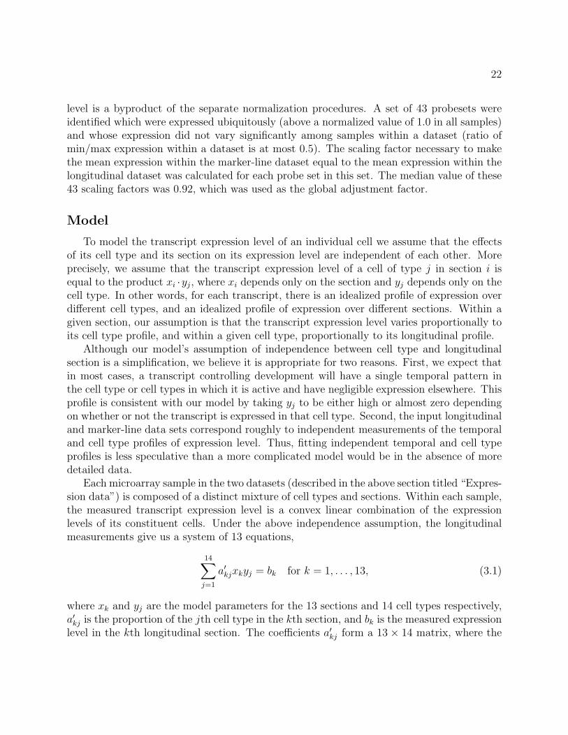
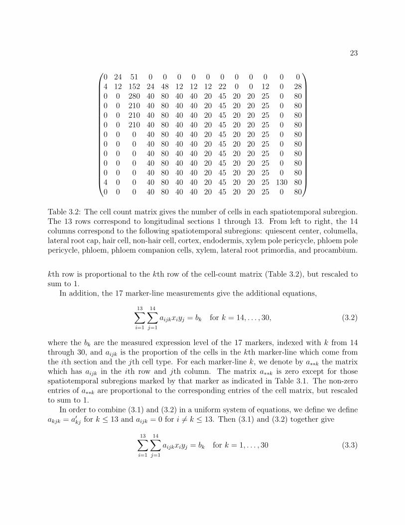
0 24 51 0 0 0 0 0 0 0 0 0 0 04 12 152 24 48 12 12 12 22 0 0 12 0 280 0 280 40 80 40 40 20 45 20 20 25 0 800 0 210 40 80 40 40 20 45 20 20 25 0 800 0 210 40 80 40 40 20 45 20 20 25 0 800 0 210 40 80 40 40 20 45 20 20 25 0 800 0 0 40 80 40 40 20 45 20 20 25 0 800 0 0 40 80 40 40 20 45 20 20 25 0 800 0 0 40 80 40 40 20 45 20 20 25 0 800 0 0 40 80 40 40 20 45 20 20 25 0 800 0 0 40 80 40 40 20 45 20 20 25 0 804 0 0 40 80 40 40 20 45 20 20 25 130 800 0 0 40 80 40 40 20 45 20 20 25 0 80

Table 3.2: The cell count matrix gives the number of cells in each spatiotemporal subregion.The 13 rows correspond to longitudinal sections 1 through 13. From left to right, the 14columns correspond to the following spatiotemporal subregions: quiescent center, columella,lateral root cap, hair cell, non-hair cell, cortex, endodermis, xylem pole pericycle, phloem polepericycle, phloem, phloem companion cells, xylem, lateral root primordia, and procambium.

kth row is proportional to the kth row of the cell-count matrix (Table 3.2), but rescaled tosum to 1.

In addition, the 17 marker-line measurements give the additional equations,

13∑i=1

14∑j=1

aijkxiyj = bk for k = 14, . . . , 30, (3.2)

where the bk are the measured expression level of the 17 markers, indexed with k from 14through 30, and aijk is the proportion of the cells in the kth marker-line which come fromthe ith section and the jth cell type. For each marker-line k, we denote by a∗∗k the matrixwhich has aijk in the ith row and jth column. The matrix a∗∗k is zero except for thosespatiotemporal subregions marked by that marker as indicated in Table 3.1. The non-zeroentries of a∗∗k are proportional to the corresponding entries of the cell matrix, but rescaledto sum to 1.

In order to combine (3.1) and (3.2) in a uniform system of equations, we define we defineakjk = a′kj for k ≤ 13 and aijk = 0 for i 6= k ≤ 13. Then (3.1) and (3.2) together give

13∑i=1

14∑j=1

aijkxiyj = bk for k = 1, . . . , 30 (3.3)

24

Cell matrix

As described in the previous section, the coefficients aijk in our model depend on thenumber of cells in each spatiotemporal subregion. These cell number estimates were gen-erated by visual inspection of successive optical cross-sections of Arabidopsis roots alongthe longitudinal axis using confocal laser scanning microscopy. For the xylem, phloem andprocambium cell types, cell counts were obtained from earlier experiments [6, 42]. Whatfollows is a detailed description of this visual and literature analysis. These results are alsosummarized in Table 3.2.

Longitudinal section 1 encompasses two tiers of 12 columella cells, and three tiers oflateral root cap cells (15, 18 and 18 moving up from the tip).

Longitudinal section 2 contains one tier of 12 columella cells and six tiers of lateral rootcap cells (20, 20, 28, 28, 28 and 28 moving up from the tip). For all other cell types in longi-tudinal section 2, three tiers of cells are present. Eight trichoblast (hair cell precursor) cellsand 16 atrichoblast (non-hair cell precursor) cells are present circumferentially throughoutthe root, resulting in 24 and 48 cells respectively in the hair cell and non-hair cell precursorfiles in longitudinal section 2. Throughout the root, eight cortex and eight endodermis cellsare present circumferentially. However in longitudinal section 2, the cortex/endodermis ini-tial is undergoing asymmetric periclinal divisions to produce the cortex and endodermis cellfiles, so we consider there to be approximately 0.5 cells of the cortex and endodermis type,resulting in 12 cells of each type in longitudinal section 2. When the Arabidopsis root isseven days old, each longitudinal section from 3–13 contains approximately five cells of eachtype along the root’s longitudinal axis.

In longitudinal section 2, the tangential and periclinal divisions that give rise to phloemcell files do not occur, but do occur in longitudinal section 3 [6]. Three cells are present inthe main xylem axis in the first tier of cells, four cells in the second tier, and five cells in thethird tier [42]. Eight procambial cells are present in the first cell tier, 12 procambial cells inthe second tier, and 18 cells in the third tier resulting in 28 procambial cells in longitudinalsection 2 [42]. For all sections xylem pole pericycle cells are the two cells that flank the xylemaxis on either end, and phloem pole pericycle cells are considered the intervening cells. Fourpericycle cells can be identified as flanking xylem cells in all three tiers of cells present inlongitudinal section 2 [42]. Seven intervening phloem pole pericycle cells can be found intier one, and eight intervening cells can be identified in the third tier [42], resulting in 22procambial cells in longitudinal section 2.

In a seven day old root, each of the longitudinal sections 3–13 contains approximatelyfive tiers of cells. In longitudinal section 3, columella cells can no longer be identified, and10 tiers of lateral root cap cells exist containing 28 cells each. In sections 4–6, a lateralroot cap cell is twice the length and half the width of an epidermal cell. Eighty-four cellswere identified in each tier, and two and a half tiers of cells exist each for longitudinalsections 4–6 resulting in 210 cells for each longitudinal section. All other cell types haveundergone the appropriate tangential and periclinal divisions to establish their respective

25

cell files by longitudinal section 3. Two protophloem cells, two metaphloem cells and fouraccompanying companion cells are present in the phloem tissue [6]. With the combinationof protophloem and metaphloem cells, 20 phloem cells and 20 companion cells exist in eachlongitudinal section. Approximately 40 procambial cells exist in each longitudinal section.Secondary cell growth does not occur in the developmental stages sampled, therefore, thisnumber remains fixed throughout all developmental stages. In longitudinal section 12, a non-emerged lateral root is hypothesized to be present based on microarray expression data [7].This lateral root is estimated to be approximately 130 cells, or one tier of cells in longitudinalsection 2.

In our modelling the distinct vasculature, protophloem and metaphloem cell types weretreated as a single cell type, as no marker-line was specific enough to differentiate clearlybetween these cell types. Also, the metaxylem and protoxylem were considered as a singlecell type by the same rationale.

Solving bilinear equations

In this section, we show how the bilinear equations given by (3.3) can be solved usingthe algorithm in Section 2.1. The equations (3.3) have the form of equation (2.1) withn = 13 + 14 = 27 and ` = 30 + 1 = 31. The extra equation beyond the 30 in (2.1) comesbecause we add a normalization condition, that

∑13i=1 xi = 1. We can take the matrix g to

have s = 2 rows and have columns(1 0

)Tfor the x variables and

(0 1

)Tfor the y variables.

Then, the system satisfies the condition the beginning of Section 2.1 with d1 = d2 = 1.For completeness, we write out the iteration steps (2.3) and (2.4) in this situation. At

each iteration, the expectation step (2.3) computes the quantities:

w(s)ijk := bk

aijkx(s)i y

(s)j∑n

i′=1

∑mj′=1 ai′j′kx

(s)i′ y

(s)j′

(3.4)

for all i, j, and k. This quantity w(s)ijk is an estimate of the contribution of the (i, j) term in

the kth equation in (3.3). We break the maximization step into first computing the analoguesof the sufficient statistics:

X(s)i =

m∑j=1

∑k=1

w(s)ijk

Y(s)j =

n∑i=1

∑k=1

w(s)ijk.

Then we perform an iteration beginning with x(s,0)i = x

(s)i and y

(s,0)j = y

(s)j and the update

26

rules

x(s,t+1)i := x

(s,t)i

X(s)i∑m

j=1

∑`k=1 aijkx

(s,t)i y

(s,t)j

y(s,t+1)j := y

(s,t)j

Y(s)j∑n

i=1

∑`k=1 aijkx

(s,t+1)i y

(s,t)j

until the parameters converge. Note that we are ignoring the normalization equation∑xi =

1. Instead, we incorporate that condition right before the next EM step by re-normalizing:

x(s+1)i :=

x(s,t)i∑n

i′=1 x(s,t)i′

y(s+1)j := y

(s,t)j

m∑i′=1

x(s,t)i′ .

Since these are just local searches which may converge only to local minima, for eachtranscript, we ran our algorithm 20 different times starting from 20 different randomly chosenstarting points. For every transcript in our data, all 20 runs of the algorithm converged tothe same solution, up to a small tolerance. We therefore believe that in almost all caseswe have found a global, and not merely local, minimum to the modified Kullback-Leiblerdivergence. Most likely, this consistency is a consequence of the particular coefficients of ourequations, and in general there may be multiple local minima.

Computational validation methodology

In order to validate our method, we simulated expression profiles according to variousmodels and tested our method’s ability to reconstruct the underlying parameters. First,we simulated data according to the same independence model defined in the Model section.The underlying spatiotemporal subregion expression levels were sampled from a log-normaldistribution with standard deviation 0.5. The simulated measurements bk were computedfrom these subregion levels according to our model of the Arabidopsis root in (3.3). Finally,multiplicative error was added, distributed according to a log-normal distribution with stan-dard deviation 0.03 to simulate measurement noise. This procedure created expression datawith varying but comparable expression levels, which we will call the “uniform” dataset.However, since we are particularly interested in genes for which the expression levels arenot uniform, we also produced simulations with the expression level for a given section orcell type raised by a factor of 10, which we will call the “elevated” dataset. In this dataset,we only measured the error for the same section or cell type which was elevated. Thesesimulations measure our ability to detect a dominant expression pattern.

27

In addition, we designed simulations that test the robustness of the algorithm to failuresof the bilinear model for root expression levels. For each section and cell type, we simulateddata in which the expression levels for cells in that section or cell type did not follow thebilinear model, and call these the “section” and “cell type” datasets respectively. Instead,the expression levels in the given section or cell type were chosen independently according toa log-normal distribution with standard deviation 0.5

√2. The factor of

√2 was introduced

because the product of two log-normally distributed numbers with standard deviation 0.5 isdistributed log-normally with standard deviation 0.5

√2.

The predictions were compared to the true expression levels across the spatiotemporalsubregions within each section and each cell type. For each section and each cell type, theexpression levels in its spatiotemporal subregions were averaged, ignoring those combinationswhich are not physically present in the root, (i.e. those whose entry in Table 3.2 is 0). Thedifference between the predicted and true average expressions was computed as a proportionof the true average expression. We then computed the root mean square of the proportionalerror over 500 simulations.

Visualization of predicted expression patterns

Predicted expression values were colored according to an Arabidopsis root template (Fig-ure 3.1). The green channel of each cell was set according to a linear mapping betweenthe expression range shown in the template [1, 10] or [1, 5] to the range [0, 255]. Expressionvalues above or below that range are given values of 255 or 0 respectively. The mapping isalso shown to the right of the false color image in the form of a gradient key. Phloem cellsby longitudinal section are visualized separately on the right hand side of the root as theyare physically occluded by other cells in the left hand side representation. The minimumand maximum range of expression value visualized can also be adjusted by the user.

In vivo validation methodology

To validate predicted expression values, we used transgenic Arabidopsis thaliana linescontaining transcriptional GFP fusions in the Columbia ecotype [39]. For each gene beingvalidated, six plants from at least two insertion lines previously described as expressingGFP were characterized. All plants were grown vertically on 1X Murashige and Skoog saltmixture, 1% sucrose and 2.3 mM 2-(N -morpholino)ethanesulfonic acid (pH 5.7) in 1% agar.Seedlings were prepared for microscopy at 5 days of age. Confocal images were obtained usinga 25x water-immersion lens on a Zeiss LSM-510 confocal laser-scanning microscope using the488-nm laser for excitation. Roots were stained with 10 µg/mL propidium iodide for 0.5 to2 minutes and mounted in water. GFP was rendered in green and propidium iodide inred. Images were saved in TIFF format. Images were manually stitched together in AdobePhotoshop CS2 using the Photomerge command. The black background surrounding the

28

root was modified to ensure uniformity across figures. No other image enhancement wasperformed.

3.2 Results

Computational validation

The root mean square percentage errors in the reconstruction of each parameter areshown in Table 3.3. In the first two columns, where the data were generated according to thebilinear model, the error rate is generally no greater than the simulated measurement error.In most cases, elevated expression led to a lower error rate. In particular, reconstruction ofexpression in procambium was much more accurate in the elevated dataset.

The last two columns show that the algorithm is robust to violations of the bilinearmodel. Also, the predicted expression level in each cell type is generally not greatly affectedby the failure of the model in other cell types, and similarly with sections.

In vivo validation

To determine whether our algorithm can accurately resolve spatiotemporal subregion-level transcript expression values, it would be ideal to compare the predictions to measuredmicroarray expression values of the same spatiotemporal subregion. However, due to techni-cal constraints, it is not possible to measure mRNA expression to such a degree of specificityand thus we cannot validate the estimates directly. Instead, we validated the method by visu-ally comparing the predicted pattern of expression to patterns obtained from transcriptionalGFP fusions using laser scanning confocal microscopy, as described in [39].

For each gene validated, a false-colored root image was generated by coloring each spa-tiotemporal subregion of an annotated Arabidopsis root template (Figure 3.1) accordingto the expression level in that subregion as predicted by our method. This false-coloredimage was then visually compared against the actual pattern of fluorescence observed inplants expressing a transcriptional GFP fusion specific for the promoter of that gene. Thesetranscriptional GFP fusions contain up to 3 kb of regulatory sequence upstream of thetranslational start site of the respective gene. In many cases, this sequence is sufficient torecapitulate endogenous mRNA expression patterns as defined by cell type resolution mi-croarray data [39]. This comparative method of validation allows us to assess the accuracy ofspatiotemporal subregion expression predictions in an efficient and technically feasible way.

As a benchmark validation test, a set of three transcriptional fusions which were used toobtain some of the marker-line dataset were examined: S18(AT5G12870 ), S4(AT3G25710 ),and S32(AT2G18380 ). These fusions were originally selected for use in profiling because theyexhibited enriched cell type expression as observed by laser scanning confocal microscopyand subsequently confirmed in the microarray expression data. The expression predictions

29

Figure 3.2: (A) Expression of AT2G18380 in all developmental stages of the phloem waspredicted by our method and visualized in a representation of the Arabidopsis root. Phloemcells are shown external to the root. (B) GFP expression in the longitudinal axis and (C)expression in cross-section of expression driven by the AT2G18380 promoter validate theprediction.

30

Error rateVariable uniform elevated cell type sectionSection 1 2.7 2.4 3.3 3.6Section 2 3.4 3.0 5.7 7.5Section 3 3.3 2.7 5.8 7.2Section 4 3.2 2.8 5.3 6.5Section 5 3.1 2.7 5.3 6.5Section 6 3.3 2.7 5.3 6.5Section 7 3.1 2.5 3.7 5.0Section 8 3.0 2.3 3.6 4.9Section 9 3.0 2.2 3.6 4.8Section 10 2.7 2.1 3.5 4.5Section 11 2.9 2.2 3.4 4.6Section 12 3.3 2.2 4.4 5.3Section 13 2.4 2.1 3.6 5.3Quiescent center 3.0 3.1 3.0 3.1Columella 3.1 3.8 4.9 4.1Lateral root cap 2.6 1.6 3.6 3.1Hair cell 3.4 2.8 9.1 4.3Non-hair cell 3.0 2.1 3.1 3.0Cortex 2.9 2.1 6.9 3.6Endodermis 2.8 2.2 3.5 3.2Xylem pole pericycle 3.3 3.1 10.8 4.9Phloem pole pericycle 3.0 2.9 9.4 4.9Phloem 3.0 2.9 3.0 3.0Phloem ccs 3.3 3.4 11.7 4.9Xylem 2.2 2.1 2.5 2.2Lateral root primordia 3.5 3.0 3.4 3.3Procambium 8.3 1.8 12.7 12.7

Table 3.3: Root mean square percentage error rates in the reconstruction of simulated data.The first column is under a model of comparable but varying expression levels across allsections and cell types. The second type is the error rate when that section or cell typehas its expression level raised by a factor of 10. The third and fourth columns show modelsin which the bilinear assumption is violated in one of the sections or one of the cell typesrespectively. In all cases, 3% measurement error has been added to the expression levels.

from our method accurately recapitulated the observed pattern of all three benchmark genes(Figure 3.2 and data not shown).

To assess the novel predictive ability of our method to reconstruct in vivo expression pat-

31

Figure 3.3: (A) Our method correctly predicts specific expression of AT4G37940 in a celltype, procambium, that is only covered by a general tissue marker, WOL. Expression con-ferred by the AT4G37940 promoter fused to GFP as a reporter was visualized in the col-umella (B) and in the procambium by a longitudinal section (B) and a cross section (C).The label X indicates the xylem axis. The expression also validates a maximal peak in themeristematic zone.

32

terns given missing data, we selected transcriptional fusions for genes for which our methodpredicts expression in cell types or in spatiotemporal subregions that were not marked byfluorescent marker-lines in the original dataset. At least two lines per transcriptional fu-sion were monitored. With respect to an unmarked cell type, our method predicted thatAT4G37940 was highly expressed in the columella and developing procambium. Imaging ofa transcriptional fusion of this gene confirmed this expression (Figure 3.3).

To determine if our method could correctly differentiate expression in a specific develop-mental stage of a cell type, we selected AT5G43040 for further analysis. The collection ofmarker-lines used to generate the original dataset included a marker for all developmentalstages of non-hair cells, composed of their precursors (atrichoblasts) and fully developednon-hair cells. However, the marker-line used for hair cells only marks mature hair cells, andnot their precursors (trichoblasts). Our method predicts AT5G43040 expression throughoutthe epidermis—in mature hair cell, trichoblast, mature non-hair cell and atrichoblast cellfiles—with higher expression predicted in non-hair cells than in hair cells. This differen-tial expression was validated using the AT5G43040 transcriptional fusion (SupplementaryFigure 2) demonstrating that our method is not only able to identify expression in a devel-opmental stage of a cell type not marked by the marker-line data, but also to accuratelydifferentiate relative levels of a transcript. However, it should be noted that expression in thetranscriptional fusion did not fully corroborate the expression predicted by our algorithm—specifically, expression was found in the lateral root cap which was not predicted by ouralgorithm.

Examination of the raw microarray expression data revealed that expression was notelevated in the lateral root cap in the input microarray data. Most likely, the presence ofGFP is not indicative of erroneous reconstruction of AT5G43040 expression in this case.Instead, the transcriptional fusion does not contain sufficient regulatory elements to directthe appropriate expression as described in [39], perhaps within downstream sequences. Forthis reason, a comparison of the ratio between raw marker line and section expression datacan be obtained as a link for each gene so that the user can simultaneously assess rawexpression data with the reconstructed expression patterns.

3.3 Discussion

We have shown that spatiotemporal patterns of gene expression in the Arabidopsis rootcan be reconstructed using information from the marker-line and longitudinal datasets. Cur-rent experimental techniques are limited in their ability to rapidly and accurately microdis-sect organs into all component cell types at all developmental stages. Our computationaltechnique helps to overcome these limitations. We fully integrate the marker-line and longi-tudinal data sets into a comprehensive expression pattern, across both space and time. Inparticular, this method has enabled the identification of Arabidopsis root procambium andtrichoblast-specific genes, which have been previously experimentally intractable cell types.

33

Our high-resolution expression patterns will allow us to better understand the regulatorylogic that controls developmental processes of the Arabidopsis root. These transcriptionalregulatory networks are key to understanding developmental processes and environmentalresponses. With only a portion of these genes and fewer cell types, high-resolution spa-tiotemporal data has been used to identify transcriptional regulatory modules [7]. Our moreaccurate and complete dataset will allow a more comprehensive discovery of regulatory net-works across additional cell types.

Moreover, we expect that our algorithm and the model which underlies it are applicable totime course experiments on other heterogeneous cell mixtures. Measurements in multicellularorganisms are taken from complex cell mixtures of organs, tissues, heterogeneous cell lines, orcancerous samples. When precise histological characterization of these samples can estimateunderlying cell type composition, our method can be used to reconstruct the underlying celltype-specific gene expression patterns or any other type of quantitative data, such as high-throughput protein abundance measurements. Theoretically, this algorithm can be appliedto identify missing data in any experimental system that captures data in two or moredimensions which are assumed to be independent of one another.

34

Chapter 4

Semi-symmetric tensor ranks

This chapter is based on this paper “Secant varieties of P2 × Pn embedded by O(1, 2),”which was jointly authored with Daniel Erman and Luke Oeding [11].

Let U , V , and W be complex vector spaces of dimension m, n, and k respectively, and letx be an element in the tensor product of of their duals, U∗⊗V ∗⊗W ∗. The border rank of x isthe minimal r such that the corresponding point [x] ∈ P(U∗⊗V ∗⊗W ∗) lies in the rth secantvariety of the Segre variety of P(U∗) × P(V ∗) × P(W ∗). Similarly, for a symmetric tensorx ∈ S3U∗ or a partially symmetric tensor x ∈ U∗⊗S2V ∗, the symmetric border rank and thepartially symmetric border rank are the smallest r such that [x] is in the rth secant variety ofthe Veronese or the Segre-Veronese variety, respectively. Developing effective techniques forcomputing and characterizing the border rank of tensors is an active area of research whichspans classical algebraic geometry and representation theory [30, 31, 32, 33, 34, 43].

In the partially symmetric case, the secant varieties of P1 × Pn−1 embedded by the linebundle O(1, 2) are closely related to standard results about pencils of symmetric matrices.Moreover, the non-symmetric analogue is P1 × Pn−1 × Pk−1 embedded by O(1, 1, 1), andthe defining equations of all of its secant varieties are known by work of Landsberg andWeyman [34, Thm. 1.1]. We record the partially symmetric analogue in Proposition 4.4.2.

The main result of this chapter is Theorem 4.4.3, which focuses on the next case: secantvarieties of P2×Pn−1 embedded by O(1, 2). We give two explicit matrices, and we prove that,when r ≤ 5, their minors and Pfaffians, respectively, generate the defining ideal for thesesecant varieties. To illustrate, fix a basis e1, e2, e3 of U∗. We may then express any pointx ∈ P(U∗⊗S2V ∗) as x = e1⊗A1+e2⊗A2+e3⊗A3 where each Ai ∈ S2V ∗ can be representedby an n × n symmetric matrix. With the ordered triplet of matrices (A1, A2, A3) servingas coordinates on P(U∗ ⊗ S2V ∗), our main result is the following, which is a restatement ofTheorem 4.4.3:

Theorem 4.0.1. Let Y be the image of P2×Pn−1 in P3(n+12 )−1 ∼= P(U∗⊗S2V ∗) embedded by

O(1, 2). For any r ≤ 5, the rth secant variety of Y is defined by the prime ideal generated

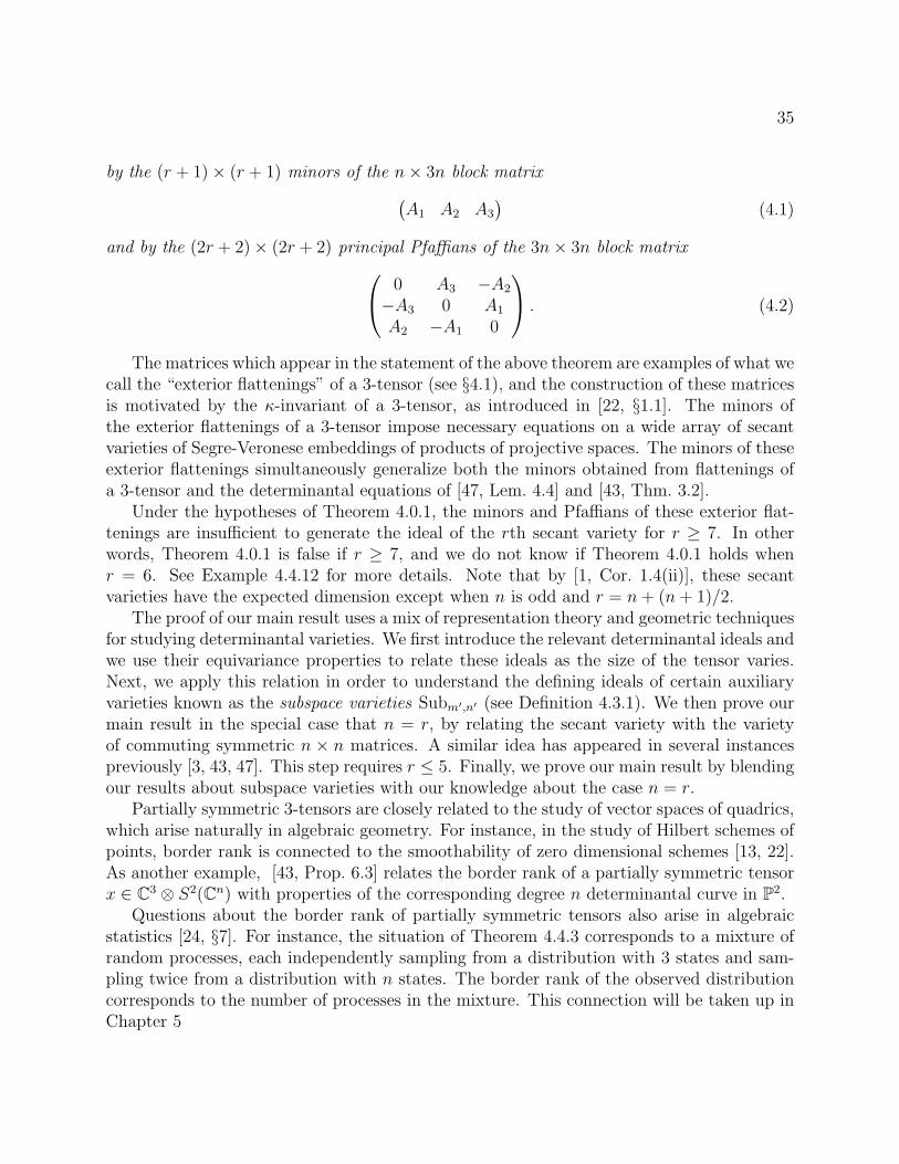
35

by the (r + 1)× (r + 1) minors of the n× 3n block matrix(A1 A2 A3

)(4.1)

and by the (2r + 2)× (2r + 2) principal Pfaffians of the 3n× 3n block matrix 0 A3 −A2

−A3 0 A1

A2 −A1 0

. (4.2)

The matrices which appear in the statement of the above theorem are examples of what wecall the “exterior flattenings” of a 3-tensor (see §4.1), and the construction of these matricesis motivated by the κ-invariant of a 3-tensor, as introduced in [22, §1.1]. The minors ofthe exterior flattenings of a 3-tensor impose necessary equations on a wide array of secantvarieties of Segre-Veronese embeddings of products of projective spaces. The minors of theseexterior flattenings simultaneously generalize both the minors obtained from flattenings ofa 3-tensor and the determinantal equations of [47, Lem. 4.4] and [43, Thm. 3.2].

Under the hypotheses of Theorem 4.0.1, the minors and Pfaffians of these exterior flat-tenings are insufficient to generate the ideal of the rth secant variety for r ≥ 7. In otherwords, Theorem 4.0.1 is false if r ≥ 7, and we do not know if Theorem 4.0.1 holds whenr = 6. See Example 4.4.12 for more details. Note that by [1, Cor. 1.4(ii)], these secantvarieties have the expected dimension except when n is odd and r = n+ (n+ 1)/2.

The proof of our main result uses a mix of representation theory and geometric techniquesfor studying determinantal varieties. We first introduce the relevant determinantal ideals andwe use their equivariance properties to relate these ideals as the size of the tensor varies.Next, we apply this relation in order to understand the defining ideals of certain auxiliaryvarieties known as the subspace varieties Subm′,n′ (see Definition 4.3.1). We then prove ourmain result in the special case that n = r, by relating the secant variety with the varietyof commuting symmetric n × n matrices. A similar idea has appeared in several instancespreviously [3, 43, 47]. This step requires r ≤ 5. Finally, we prove our main result by blendingour results about subspace varieties with our knowledge about the case n = r.

Partially symmetric 3-tensors are closely related to the study of vector spaces of quadrics,which arise naturally in algebraic geometry. For instance, in the study of Hilbert schemes ofpoints, border rank is connected to the smoothability of zero dimensional schemes [13, 22].As another example, [43, Prop. 6.3] relates the border rank of a partially symmetric tensorx ∈ C3 ⊗ S2(Cn) with properties of the corresponding degree n determinantal curve in P2.

Questions about the border rank of partially symmetric tensors also arise in algebraicstatistics [24, §7]. For instance, the situation of Theorem 4.4.3 corresponds to a mixture ofrandom processes, each independently sampling from a distribution with 3 states and sam-pling twice from a distribution with n states. The border rank of the observed distributioncorresponds to the number of processes in the mixture. This connection will be taken up inChapter 5

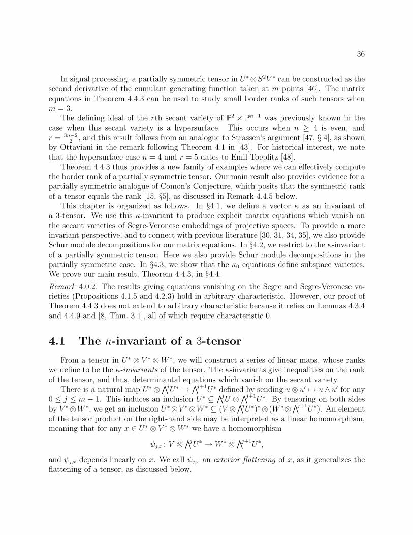
36

In signal processing, a partially symmetric tensor in U∗⊗S2V ∗ can be constructed as thesecond derivative of the cumulant generating function taken at m points [46]. The matrixequations in Theorem 4.4.3 can be used to study small border ranks of such tensors whenm = 3.

The defining ideal of the rth secant variety of P2 × Pn−1 was previously known in thecase when this secant variety is a hypersurface. This occurs when n ≥ 4 is even, andr = 3n−2

2, and this result follows from an analogue to Strassen’s argument [47, § 4], as shown

by Ottaviani in the remark following Theorem 4.1 in [43]. For historical interest, we notethat the hypersurface case n = 4 and r = 5 dates to Emil Toeplitz [48].

Theorem 4.4.3 thus provides a new family of examples where we can effectively computethe border rank of a partially symmetric tensor. Our main result also provides evidence for apartially symmetric analogue of Comon’s Conjecture, which posits that the symmetric rankof a tensor equals the rank [15, §5], as discussed in Remark 4.4.5 below.

This chapter is organized as follows. In §4.1, we define a vector κ as an invariant ofa 3-tensor. We use this κ-invariant to produce explicit matrix equations which vanish onthe secant varieties of Segre-Veronese embeddings of projective spaces. To provide a moreinvariant perspective, and to connect with previous literature [30, 31, 34, 35], we also provideSchur module decompositions for our matrix equations. In §4.2, we restrict to the κ-invariantof a partially symmetric tensor. Here we also provide Schur module decompositions in thepartially symmetric case. In §4.3, we show that the κ0 equations define subspace varieties.We prove our main result, Theorem 4.4.3, in §4.4.

Remark 4.0.2. The results giving equations vanishing on the Segre and Segre-Veronese va-rieties (Propositions 4.1.5 and 4.2.3) hold in arbitrary characteristic. However, our proof ofTheorem 4.4.3 does not extend to arbitrary characteristic because it relies on Lemmas 4.3.4and 4.4.9 and [8, Thm. 3.1], all of which require characteristic 0.

4.1 The κ-invariant of a 3-tensor

From a tensor in U∗ ⊗ V ∗ ⊗W ∗, we will construct a series of linear maps, whose rankswe define to be the κ-invariants of the tensor. The κ-invariants give inequalities on the rankof the tensor, and thus, determinantal equations which vanish on the secant variety.

There is a natural map U∗ ⊗∧jU∗ → ∧j+1U∗ defined by sending u⊗ u′ 7→ u∧ u′ for any

0 ≤ j ≤ m− 1. This induces an inclusion U∗ ⊆∧jU ⊗∧j+1U∗. By tensoring on both sides

by V ∗⊗W ∗, we get an inclusion U∗⊗V ∗⊗W ∗ ⊆ (V ⊗∧jU∗)∗⊗ (W ∗⊗

∧j+1U∗). An elementof the tensor product on the right-hand side may be interpreted as a linear homomorphism,meaning that for any x ∈ U∗ ⊗ V ∗ ⊗W ∗ we have a homomorphism

ψj,x : V ⊗∧jU∗ → W ∗ ⊗

∧j+1U∗,

and ψj,x depends linearly on x. We call ψj,x an exterior flattening of x, as it generalizes theflattening of a tensor, as discussed below.

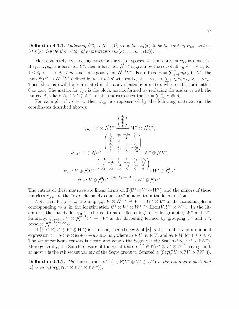
37

Definition 4.1.1. Following [22, Defn. 1.1], we define κj(x) to be the rank of ψj,x, and welet κ(x) denote the vector of κ-invariants (κ0(x), . . . , κm−1(x)).

More concretely, by choosing bases for the vector spaces, we can represent ψj,x as a matrix.If e1, . . . , em is a basis for U∗, then a basis for

∧jU∗ is given by the set of all ei1 ∧ . . .∧ eij for

1 ≤ i1 < · · · < ij ≤ m, and analogously for∧j+1U∗. For a fixed u =

∑mk=1 ukek in U∗, the

map∧jU∗ → ∧j+1U∗ defined by u′ 7→ u∧u′ will send ei1∧ . . .∧eij to

∑k uk ek∧ei1∧ . . .∧eij .

Thus, this map will be represented in the above bases by a matrix whose entries are either0 or ±ui. The matrix for ψj,x is the block matrix formed by replacing the scalar ui with thematrix Ai where Ai ∈ V ∗ ⊗W ∗ are the matrices such that x =

∑mi=1 ei ⊗ Ai.

For example, if m = 4, then ψj,x are represented by the following matrices (in thecoordinates described above):

ψ0,x : V ⊗∧0U∗

0@A1A2A3A4

1A−−−−→ W ∗ ⊗

∧1U∗,

ψ1,x : V ⊗∧1U∗

0BBB@0 A3 −A2 0−A3 0 A1 0A2 −A1 0 0A4 0 0 −A10 A4 0 −A20 0 A4 −A3

1CCCA−−−−−−−−−−−−−−→ W ∗ ⊗

∧2U∗,

ψ2,x : V ⊗∧2U∗

0@−A4 0 0 0 A3 −A20 −A4 0 −A3 0 A10 0 −A4 A2 −A1 0A1 A2 A3 0 0 0

1A−−−−−−−−−−−−−−−−−−−−→ W ∗ ⊗

∧3U∗

ψ3,x : V ⊗∧3U∗

(A1 A2 A3 A4 )−−−−−−−−−→W ∗ ⊗∧4U∗.

The entries of these matrices are linear forms on P(U∗ ⊗ V ∗ ⊗W ∗), and the minors of thesematrices ψj,x are the “explicit matrix equations” alluded to in the introduction.

Note that for j = 0, the map ψ0 : V ⊗∧0U∗ ∼= V → W ∗ ⊗ U∗ is the homomorphism

corresponding to x in the identification U∗ ⊗ V ∗ ⊗ W ∗ ∼= Hom(V, U∗ ⊗ W ∗). In the lit-erature, the matrix for ψ0 is referred to as a “flattening” of x by grouping W ∗ and U∗.Similarly, ψm−1,x : V ⊗

∧m−1U∗ → W ∗ is the flattening formed by grouping U∗ and V ∗,because

∧m−1U∗ ∼= U .If [x] ∈ P(U∗ ⊗ V ∗ ⊗W ∗) is a tensor, then the rank of [x] is the number r in a minimal

expression x = u1⊗v1⊗w1+· · ·+ur⊗vr⊗wr, where ui ∈ U , vi ∈ V , and wi ∈ W for 1 ≤ i ≤ r.The set of rank-one tensors is closed and equals the Segre variety Seg(PU∗ × PV ∗ × PW ∗).More generally, the Zariski closure of the set of tensors [x] ∈ P(U∗ ⊗ V ∗ ⊗W ∗) having rankat most r is the rth secant variety of the Segre product, denoted σr(Seg(PU∗×PV ∗×PW ∗)).

Definition 4.1.2. The border rank of [x] ∈ P(U∗ ⊗ V ∗ ⊗W ∗) is the minimal r such that[x] is in σr(Seg(PU∗ × PV ∗ × PW ∗)).

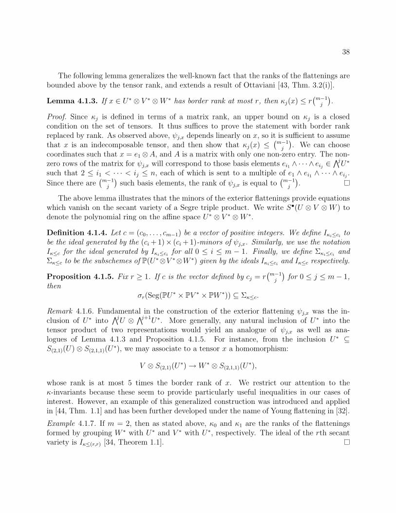
38

The following lemma generalizes the well-known fact that the ranks of the flattenings arebounded above by the tensor rank, and extends a result of Ottaviani [43, Thm. 3.2(i)].

Lemma 4.1.3. If x ∈ U∗ ⊗ V ∗ ⊗W ∗ has border rank at most r, then κj(x) ≤ r(m−1j

).

Proof. Since κj is defined in terms of a matrix rank, an upper bound on κj is a closedcondition on the set of tensors. It thus suffices to prove the statement with border rankreplaced by rank. As observed above, ψj,x depends linearly on x, so it is sufficient to assumethat x is an indecomposable tensor, and then show that κj(x) ≤

(m−1j

). We can choose

coordinates such that x = e1⊗A, and A is a matrix with only one non-zero entry. The non-zero rows of the matrix for ψj,x will correspond to those basis elements ei1 ∧ · · · ∧ eij ∈

∧jU∗such that 2 ≤ i1 < · · · < ij ≤ n, each of which is sent to a multiple of e1 ∧ ei1 ∧ · · · ∧ eij .Since there are

(m−1j

)such basis elements, the rank of ψj,x is equal to

(m−1j

).

The above lemma illustrates that the minors of the exterior flattenings provide equationswhich vanish on the secant variety of a Segre triple product. We write S•(U ⊗ V ⊗W ) todenote the polynomial ring on the affine space U∗ ⊗ V ∗ ⊗W ∗.

Definition 4.1.4. Let c = (c0, . . . , cm−1) be a vector of positive integers. We define Iκi≤ci tobe the ideal generated by the (ci + 1)× (ci + 1)-minors of ψj,x. Similarly, we use the notationIκ≤c for the ideal generated by Iκi≤ci for all 0 ≤ i ≤ m − 1. Finally, we define Σκi≤ci andΣκ≤c to be the subschemes of P(U∗⊗V ∗⊗W ∗) given by the ideals Iκi≤ci and Iκ≤c respectively.

Proposition 4.1.5. Fix r ≥ 1. If c is the vector defined by cj = r(m−1j

)for 0 ≤ j ≤ m− 1,

thenσr(Seg(PU∗ × PV ∗ × PW ∗)) ⊆ Σκ≤c.

Remark 4.1.6. Fundamental in the construction of the exterior flattening ψj,x was the in-clusion of U∗ into

∧jU ⊗ ∧j+1U∗. More generally, any natural inclusion of U∗ into thetensor product of two representations would yield an analogue of ψj,x as well as ana-logues of Lemma 4.1.3 and Proposition 4.1.5. For instance, from the inclusion U∗ ⊆S(2,1)(U)⊗ S(2,1,1)(U

∗), we may associate to a tensor x a homomorphism:

V ⊗ S(2,1)(U∗)→ W ∗ ⊗ S(2,1,1)(U

∗),

whose rank is at most 5 times the border rank of x. We restrict our attention to theκ-invariants because these seem to provide particularly useful inequalities in our cases ofinterest. However, an example of this generalized construction was introduced and appliedin [44, Thm. 1.1] and has been further developed under the name of Young flattening in [32].

Example 4.1.7. If m = 2, then as stated above, κ0 and κ1 are the ranks of the flatteningsformed by grouping W ∗ with U∗ and V ∗ with U∗, respectively. The ideal of the rth secantvariety is Iκ≤(r,r) [34, Theorem 1.1].

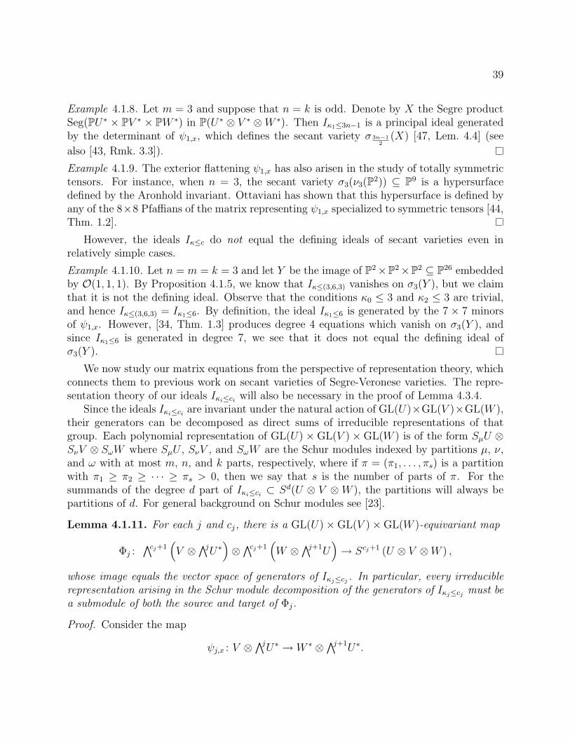
39

Example 4.1.8. Let m = 3 and suppose that n = k is odd. Denote by X the Segre productSeg(PU∗ × PV ∗ × PW ∗) in P(U∗ ⊗ V ∗ ⊗W ∗). Then Iκ1≤3n−1 is a principal ideal generatedby the determinant of ψ1,x, which defines the secant variety σ 3n−1

2(X) [47, Lem. 4.4] (see

also [43, Rmk. 3.3]).

Example 4.1.9. The exterior flattening ψ1,x has also arisen in the study of totally symmetrictensors. For instance, when n = 3, the secant variety σ3(ν3(P2)) ⊆ P9 is a hypersurfacedefined by the Aronhold invariant. Ottaviani has shown that this hypersurface is defined byany of the 8×8 Pfaffians of the matrix representing ψ1,x specialized to symmetric tensors [44,Thm. 1.2].

However, the ideals Iκ≤c do not equal the defining ideals of secant varieties even inrelatively simple cases.

Example 4.1.10. Let n = m = k = 3 and let Y be the image of P2×P2×P2 ⊆ P26 embeddedby O(1, 1, 1). By Proposition 4.1.5, we know that Iκ≤(3,6,3) vanishes on σ3(Y ), but we claimthat it is not the defining ideal. Observe that the conditions κ0 ≤ 3 and κ2 ≤ 3 are trivial,and hence Iκ≤(3,6,3) = Iκ1≤6. By definition, the ideal Iκ1≤6 is generated by the 7 × 7 minorsof ψ1,x. However, [34, Thm. 1.3] produces degree 4 equations which vanish on σ3(Y ), andsince Iκ1≤6 is generated in degree 7, we see that it does not equal the defining ideal ofσ3(Y ).

We now study our matrix equations from the perspective of representation theory, whichconnects them to previous work on secant varieties of Segre-Veronese varieties. The repre-sentation theory of our ideals Iκi≤ci will also be necessary in the proof of Lemma 4.3.4.

Since the ideals Iκi≤ci are invariant under the natural action of GL(U)×GL(V )×GL(W ),their generators can be decomposed as direct sums of irreducible representations of thatgroup. Each polynomial representation of GL(U)× GL(V )× GL(W ) is of the form SµU ⊗SνV ⊗ SωW where SµU , SνV , and SωW are the Schur modules indexed by partitions µ, ν,and ω with at most m, n, and k parts, respectively, where if π = (π1, . . . , πs) is a partitionwith π1 ≥ π2 ≥ · · · ≥ πs > 0, then we say that s is the number of parts of π. For thesummands of the degree d part of Iκi≤ci ⊂ Sd(U ⊗ V ⊗W ), the partitions will always bepartitions of d. For general background on Schur modules see [23].

Lemma 4.1.11. For each j and cj, there is a GL(U)×GL(V )×GL(W )-equivariant map

Φj :∧cj+1

(V ⊗

∧jU∗)⊗∧cj+1(W ⊗

∧j+1U)→ Scj+1 (U ⊗ V ⊗W ) ,

whose image equals the vector space of generators of Iκj≤cj . In particular, every irreduciblerepresentation arising in the Schur module decomposition of the generators of Iκj≤cj must bea submodule of both the source and target of Φj.

Proof. Consider the map

ψj,x : V ⊗∧jU∗ → W ∗ ⊗

∧j+1U∗.

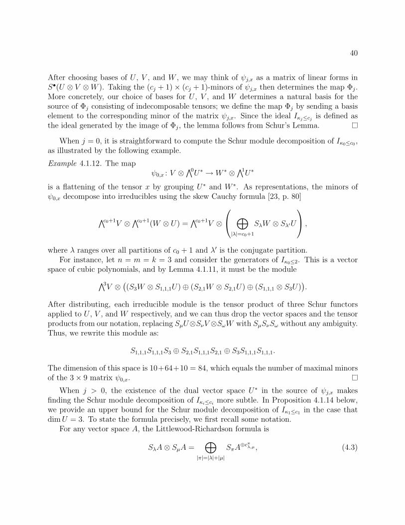
40

After choosing bases of U , V , and W , we may think of ψj,x as a matrix of linear forms inS•(U ⊗ V ⊗W ). Taking the (cj + 1)× (cj + 1)-minors of ψj,x then determines the map Φj.More concretely, our choice of bases for U , V , and W determines a natural basis for thesource of Φj consisting of indecomposable tensors; we define the map Φj by sending a basiselement to the corresponding minor of the matrix ψj,x. Since the ideal Iκj≤cj is defined asthe ideal generated by the image of Φj, the lemma follows from Schur’s Lemma.

When j = 0, it is straightforward to compute the Schur module decomposition of Iκ0≤c0 ,as illustrated by the following example.

Example 4.1.12. The mapψ0,x : V ⊗

∧0U∗ → W ∗ ⊗∧1U∗

is a flattening of the tensor x by grouping U∗ and W ∗. As representations, the minors ofψ0,x decompose into irreducibles using the skew Cauchy formula [23, p. 80]

∧c0+1V ⊗∧c0+1(W ⊗ U) =

∧c0+1V ⊗

⊕|λ|=c0+1

SλW ⊗ Sλ′U

,

where λ ranges over all partitions of c0 + 1 and λ′ is the conjugate partition.For instance, let n = m = k = 3 and consider the generators of Iκ0≤2. This is a vector

space of cubic polynomials, and by Lemma 4.1.11, it must be the module∧3V ⊗((S3W ⊗ S1,1,1U)⊕ (S2,1W ⊗ S2,1U)⊕ (S1,1,1 ⊗ S3U)

).

After distributing, each irreducible module is the tensor product of three Schur functorsapplied to U , V , and W respectively, and we can thus drop the vector spaces and the tensorproducts from our notation, replacing SµU⊗SνV ⊗SωW with SµSνSω without any ambiguity.Thus, we rewrite this module as:

S1,1,1S1,1,1S3 ⊕ S2,1S1,1,1S2,1 ⊕ S3S1,1,1S1,1,1.

The dimension of this space is 10+64+10 = 84, which equals the number of maximal minorsof the 3× 9 matrix ψ0,x.

When j > 0, the existence of the dual vector space U∗ in the source of ψj,x makesfinding the Schur module decomposition of Iκi≤ci more subtle. In Proposition 4.1.14 below,we provide an upper bound for the Schur module decomposition of Iκ1≤c1 in the case thatdimU = 3. To state the formula precisely, we first recall some notation.

For any vector space A, the Littlewood-Richardson formula is

SλA⊗ SµA =⊕

|π|=|λ|+|µ|

SπA⊕cπλ,µ , (4.3)

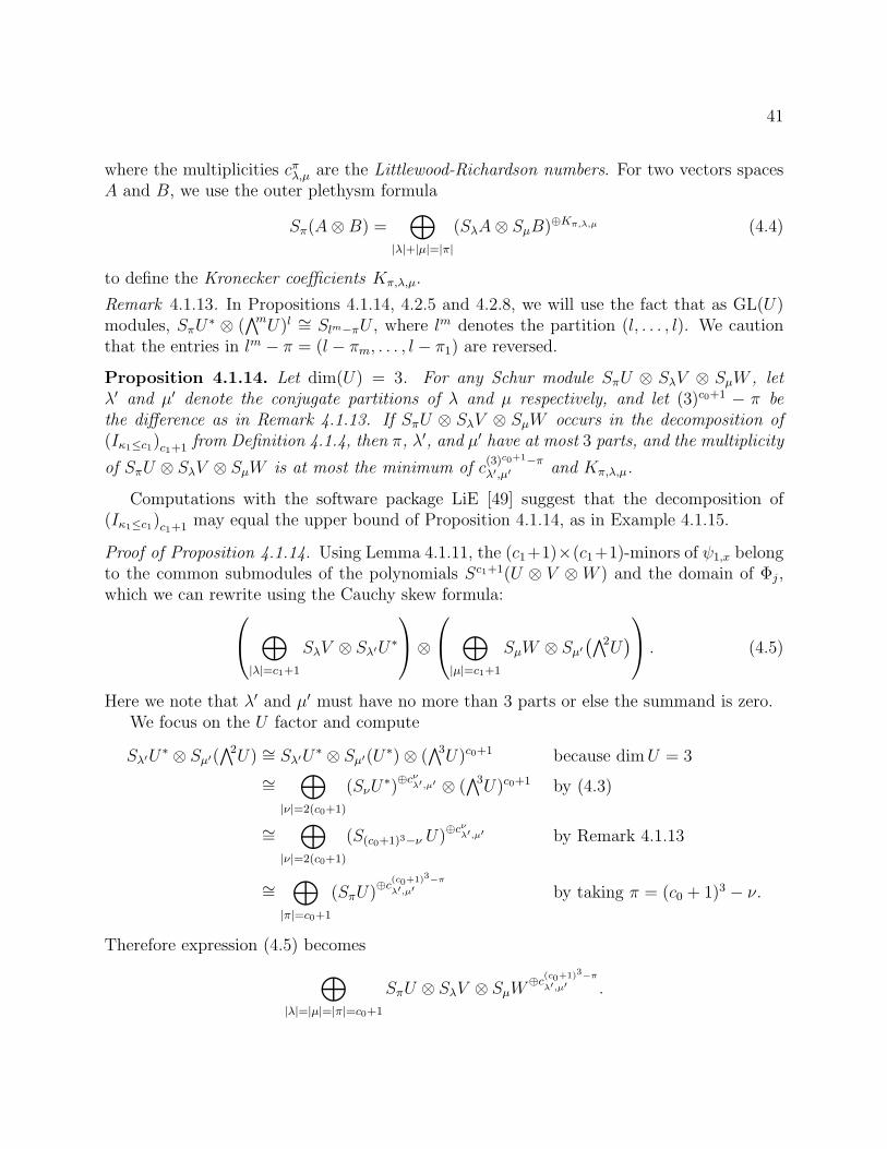
41

where the multiplicities cπλ,µ are the Littlewood-Richardson numbers. For two vectors spacesA and B, we use the outer plethysm formula

Sπ(A⊗B) =⊕

|λ|+|µ|=|π|

(SλA⊗ SµB)⊕Kπ,λ,µ (4.4)

to define the Kronecker coefficients Kπ,λ,µ.

Remark 4.1.13. In Propositions 4.1.14, 4.2.5 and 4.2.8, we will use the fact that as GL(U)modules, SπU

∗ ⊗ (∧mU)l ∼= Slm−πU , where lm denotes the partition (l, . . . , l). We caution

that the entries in lm − π = (l − πm, . . . , l − π1) are reversed.

Proposition 4.1.14. Let dim(U) = 3. For any Schur module SπU ⊗ SλV ⊗ SµW , letλ′ and µ′ denote the conjugate partitions of λ and µ respectively, and let (3)c0+1 − π bethe difference as in Remark 4.1.13. If SπU ⊗ SλV ⊗ SµW occurs in the decomposition of(Iκ1≤c1)c1+1 from Definition 4.1.4, then π, λ′, and µ′ have at most 3 parts, and the multiplicity

of SπU ⊗ SλV ⊗ SµW is at most the minimum of c(3)c0+1−πλ′,µ′ and Kπ,λ,µ.

Computations with the software package LiE [49] suggest that the decomposition of(Iκ1≤c1)c1+1 may equal the upper bound of Proposition 4.1.14, as in Example 4.1.15.

Proof of Proposition 4.1.14. Using Lemma 4.1.11, the (c1+1)×(c1+1)-minors of ψ1,x belongto the common submodules of the polynomials Sc1+1(U ⊗ V ⊗W ) and the domain of Φj,which we can rewrite using the Cauchy skew formula: ⊕

|λ|=c1+1

SλV ⊗ Sλ′U∗⊗

⊕|µ|=c1+1

SµW ⊗ Sµ′(∧2U

) . (4.5)

Here we note that λ′ and µ′ must have no more than 3 parts or else the summand is zero.We focus on the U factor and compute

Sλ′U∗ ⊗ Sµ′(

∧2U) ∼= Sλ′U∗ ⊗ Sµ′(U∗)⊗ (

∧3U)c0+1 because dimU = 3

∼=⊕

|ν|=2(c0+1)

(SνU∗)⊕cν

λ′,µ′ ⊗ (∧3U)c0+1 by (4.3)

∼=⊕

|ν|=2(c0+1)

(S(c0+1)3−ν U)⊕cν

λ′,µ′ by Remark 4.1.13

∼=⊕

|π|=c0+1

(SπU)⊕c(c0+1)3−π

λ′,µ′ by taking π = (c0 + 1)3 − ν.

Therefore expression (4.5) becomes⊕|λ|=|µ|=|π|=c0+1

SπU ⊗ SλV ⊗ SµW⊕c(c0+1)3−πλ′,µ′ .

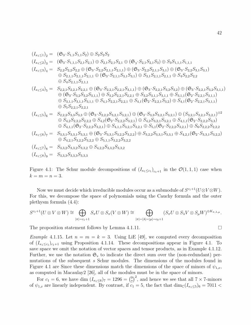
42

(Iκ1≤1)2 = (S3 ·S1,1S1,1S2)⊕ S2S2S2

(Iκ1≤2)3 = (S3 ·S1,1,1S2,1S2,1)⊕ S2,1S2,1S2,1 ⊕ (S3 ·S2,1S2,1S3)⊕ S3S1,1,1S1,1,1

(Iκ1≤3)4 = S2,2S2,2S2,2 ⊕ (S3 ·S2,2S2,1,1S2,1,1)⊕ (S3 ·S2,2S2,1,1S3,1)⊕ (S3 ·S2,2S3,1S3,1)⊕ S2,1,1S2,1,1S2,1,1 ⊕ (S3 ·S2,1,1S3,1S3,1)⊕ S3,1S2,1,1S2,1,1 ⊕ S4S2,2S2,2

⊕ S4S2,1,1S2,1,1

(Iκ1≤4)5 = S2,2,1S2,2,1S2,2,1 ⊕ (S3 ·S2,2,1S2,2,1S3,1,1)⊕ (S3 ·S2,2,1S3,2S3,2)⊕ (S3 ·S2,2,1S3,2S3,1,1)⊕ (S3 ·S3,2S3,2S3,1,1)⊕ S3,2S2,2,1S2,2,1 ⊕ S3,2S3,1,1S3,1,1 ⊕ S3,1,1(S2 ·S2,2,1S3,1,1)⊕ S3,1,1S3,1,1S3,1,1 ⊕ S4,1S2,2,1S2,2,1 ⊕ S4,1(S2 ·S2,2,1S3,2)⊕ S4,1(S2 ·S2,2,1S3,1,1)⊕ S5S2,2,1S2,2,1

(Iκ1≤5)6 = S2,2,2S3,3S3,3 ⊕ (S3 ·S2,2,2S3,2,1S3,2,1)⊕ (S3 ·S3,3S3,2,1S3,2,1)⊕ (S3,2,1S3,2,1S3,2,1)⊕2

⊕ S4,2S2,2,2S2,2,2 ⊕ S4,2(S2 ·S2,2,2S3,2,1)⊕ S4,2S3,2,1S3,2,1 ⊕ S4,1,1(S2 ·S2,2,2S3,3)⊕ S4,1,1(S2 ·S2,2,2S3,2,1)⊕ S4,1,1S3,2,1S3,2,1 ⊕ S5,1(S2 ·S2,2,2S3,2,1)⊕ S6S2,2,2S2,2,2

(Iκ1≤6)7 = S3,3,1S3,3,1S3,3,1 ⊕ (S3 ·S3,3,1S3,2,2S3,2,2)⊕ S3,2,2S3,3,1S3,3,1 ⊕ S4,2,1(S2 ·S3,3,1S3,2,2)⊕ S4,2,1S3,2,2S3,2,2 ⊕ S5,1,1S3,2,2S3,2,2

(Iκ1≤7)8 = S3,3,2S3,3,2S3,3,2 ⊕ S4,2,2S3,3,2S3,3,2

(Iκ1≤8)9 = S3,3,3S3,3,3S3,3,3

Figure 4.1: The Schur module decompositions of (Iκ1≤c1)c1+1 in the O(1, 1, 1) case when

k = m = n = 3.

Now we must decide which irreducible modules occur as a submodule of Sc1+1(U⊗V ⊗W ).For this, we decompose the space of polynomials using the Cauchy formula and the outerplethysm formula (4.4):

Sc1+1(U ⊗ V ⊗W ) ∼=⊕

|π|=c1+1

SπU ⊗ Sπ(V ⊗W ) ∼=⊕

|π|=|λ|=|µ|=c0+1

(SπU ⊗ SλV ⊗ SµW )⊕Kπ,λ,µ .

The proposition statement follows by Lemma 4.1.11.

Example 4.1.15. Let n = m = k = 3. Using LiE [49], we computed every decompositionof (Iκ1≤c1)c1+1 using Proposition 4.1.14. These decompositions appear in Figure 4.1. Tosave space we omit the notation of vector spaces and tensor products, as in Example 4.1.12.Further, we use the notation Ss to indicate the direct sum over the (non-redundant) per-mutations of the subsequent s Schur modules. The dimensions of the modules found inFigure 4.1 are Since these dimensions match the dimensions of the space of minors of ψ1,x,as computed in Macaulay2 [26], all of the modules must be in the space of minors.

For c1 = 6, we have dim (Iκ1≤6)7 = 1296 =(97

)2, and hence we see that all 7 × 7-minors

of ψ1,x are linearly independent. By contrast, if c1 = 5, the fact that dimC(Iκ1≤5)6 = 7011 <

43

7056 =(96

)2tells us that the 6 × 6 minors of ψ1,x are not all linearly independent. For

example, the upper right and lower left 6× 6 minors of

ψ1,x =

0 A3 −A2

−A3 0 A1

A2 −A1 0

are both equal to det(A1) · det(A3).

In the next section we impose partial symmetry on our 3-tensors. We remark that wecould impose other types of symmetry and this would lead to different investigations. Forinstance, we could restrict attention to 3-tensors in any of the following cases: S3(U∗),U∗ ⊗

∧2V ∗,∧3V ∗, or S2,1U

∗. In these cases, it would be straightforward to prove analoguesof Lemma 4.1.3 and Proposition 4.1.5. However, if we hope to produce the ideal definingthe appropriate secant varieties, then it is less obvious how to generalize Definition 4.1.4.It might be interesting to investigate the secant varieties of these other special types of3-tensors.

4.2 The κ-invariant for partially symmetric 3-tensors

For the rest of the chapter, we take W = V and focus on partially symmetric 3-tensorsx ∈ U∗ ⊗ S2V ∗ ⊂ U∗ ⊗ V ∗ ⊗ V ∗. By this latter inclusion, we may extend the definitionof κj(x) to partially symmetric tensors. Not only does the κ-invariant provide a bound forthe rank of x, but also for the partially symmetric rank, which is defined as the minimalr such that x =

∑ri=1 ui ⊗ vi ⊗ vi, for some ui ∈ U∗ and vi ∈ V ∗. The set of rank-one

partially symmetric tensors is known as the Segre-Veronese variety of PU∗×PV ∗ embeddedby O(1, 2). Therefore, the Zariski closure of the set of partially symmetric tensors of rankat most r is the rth secant variety of the Segre-Veronese variety. We have the followinganalogue of Definition 4.1.2.

Definition 4.2.1. The partially symmetric border rank of [x] ∈ P(U∗⊗S2V ∗) is the minimalr such that [x] is in σr(Seg(PU∗ × v2(PV ∗))).

Providing an analogue of the equations from Definition 4.1.4 is a bit more subtle whenrestricted to partially symmetric 3-tensors. In fact, it is necessary to refine the equationsif we hope to produce ideals which are radical. To see this, consider the case where x is apartially symmetric 3 × n × n tensor. For such an x, the matrix representing ψ1,x has theform

ψ1,x =

0 A3 −A2

−A3 0 A1

A2 −A1 0

where the Ai are symmetric n × n-matrices. Since ψ1,x is a skew-symmetric matrix, all ofthe principal minors in Iκ1≤c1 are squares.

44

More generally, if m = 4j + 3, then ψ2j+1,x : V ⊗∧2j+1U∗ → V ∗⊗

∧2j+2U∗ is representedby a skew-symmetric matrix in appropriate coordinates. Thus, the condition that ψ2j+1,x

has rank at most an even integer c2j+1 is defined algebraically by the principal (c2j+1 +2) × (c2j+1 + 2)-Pfaffians of ψ2j+1,x. These Pfaffians have degree c2j+1/2 + 1, whereas the(c2j+1 + 1)× (c2j+1 + 1)-minors have degree c2j+1 + 1.

To encode this skew-symmetry into our matrix equations in the case of partially sym-metric tensors, we introduce the following analogue of Definition 4.1.4.

Definition 4.2.2. Let Iκj≤cj in S•(U ⊗ S2V ) denote the ideal generated by the (cj + 2) ×(cj + 2)-Pfaffians of ψj,x, if j = (m − 1)/2, j is an odd integer, and cj is even. Otherwise,Iκj≤cj denotes the specialization of the ideal in Definition 4.1.4. As in Definition 4.1.4, for avector c, Iκ≤c is defined to be the ideal generated by the Iκj≤cj for all j, and Σκi≤ci and Σκ≤care the subschemes of P(U∗ ⊗ S2V ∗) defined by Iκi≤ci and Iκ≤c respectively.

Note that for partially symmetric tensors x, we have κj(x) = κm−1−j(x) and likewiseIκj(x)≤cj = Iκm−1−j≤cj for all j. With notation in Definition 4.2.2, we also obtain the followinganalogue of Proposition 4.1.5.

Proposition 4.2.3. Fix r ≥ 1. Let X be the Segre-Veronese variety of P(U∗) × P(V ∗) inP(U∗ ⊗ S2V ∗) and let c be the vector defined by cj = r

(m−1j

)for 0 ≤ j ≤ m − 1. Then

σr(X) ⊆ Σκ≤c.

Remark 4.2.4. Although the rest of this chapter concerns partially symmetric 3×n×n tensors,we note that the equations given in Definition 4.2.2 would be insufficient to generate the idealof the secant varieties for m ≥ 4. For example, consider the space of partially symmetric4× n× n tensors. If x is such a tensor, then the matrix representing ψ2,x has the form

ψ2,x =

−A4 0 0 0 A3 −A2

0 −A4 0 −A3 0 A1

0 0 −A4 A2 −A1 0A1 A2 A3 0 0 0

where each Ai is an n × n symmetric matrix. If x has border rank at most r, then ψ1,x

will have rank at most 3r by Proposition 4.2.3. However, the bold submatrix in the upperright will have rank at most 2r. Moreover, since the bold submatrix is skew-symmetric, thecondition that it has rank at most 2r is given by the vanishing of its (2r + 2) × (2r + 2)-principal Pfaffians. Thus, the defining ideal of the rth secant variety must contain thesePfaffians, as well as 3 other sets of Pfaffians which arise by symmetry. Since the Pfaffianshave degree r + 1, they can not be in the ideal of the (3r + 1)× (3r + 1)-minors.

In effect, these Pfaffians amount to the generators of Iκ1≤2r applied to a 3 × n × nsubtensor. In the literature on tensors, this process for producing equations on larger tensorsby applying known equations to all subtensors is known as inheritance. See [31, §2.1] for aprecise definition in the language of representation theory. The above analysis shows how theinheritance of κ-equations can produce new equations beyond the κ-equations themselves.

45

Proposition 4.2.5. As a Schur module, we have the following decomposition of the gener-ators Iκ0≤r into irreducible representations of GL(U)×GL(V )

(Iκ0≤r)r+1 =⊕|π|=r+1

SπU ⊗ Sπ′+1r+1V,

where π′ is the conjugate partition to π, and 1r+1 = (1, . . . , 1) is the partition with r + 1parts.

In the proof, we will need the following observation.

Lemma 4.2.6. Suppose π is a partition of d and suppose A is a vector space. If SλA is amodule occurring in the decomposition of Sπ(S2A) then λ has at most d parts.

Proof. Since π is a partition of d, we have an inclusion Sπ(S2A) ⊂ (S2A)⊗d. By inductivelyapplying the Pieri formula to (S2A)⊗d = (S2A)⊗d−1 ⊗ S2A, we see that every module in thedecomposition of (S2A)⊗d can have at most d parts.

Proof of Proposition 4.2.5. After choosing bases of U and V , we may view the map ψ0,x asa matrix of linear forms in S•(U ⊗ S2V ). By Lemma 4.1.11, (Iκ0≤r)r+1 is the image of theGL(U)×GL(V )-equivariant morphism

Φ0 :∧r+1V ⊗

∧r+1 (U ⊗ V )→ Sr+1(U ⊗ S2(V )),

which sends an indecomposable basis element in the source to the corresponding minor in thepolynomial ring. The first step of our proof is to show that only those representations of theform SπU⊗Sπ′+1r+1V appear in both the source and target of Φ0. By Schur’s Lemma, this willprovide a necessary condition on the representations which can appear in the decompositionof (Iκ0≤r)r+1. The second step of our proof is to show that each such representation actuallyarises; for this, we produce an explicit nonzero minor of ψ0,x that is in the image of Φ0

restricted to SπU ⊗ Sπ′+1r+1V , so that Φ0 restricted to SπU ⊗ Sπ′+1r+1V is nonzero.For the first step, suppose that SπU⊗SλV is a module in Sr+1(U⊗S2V ). If we apply the

Cauchy decomposition formula to Sd(U⊗S2V ), and consider the resulting modules as GL(U)-representations, then we must have SπU ⊗ SλV contained in the summand SπU ⊗ Sπ(S2V ).In particular we must have SλV ⊂ Sπ(S2V ). Therefore, by Lemma 4.2.6, λ has at most r+1parts.

On the other hand, we can use the skew Cauchy formula to decompose∧r+1V ⊗∧r+1(U ⊗ V ) =

∧r+1V ⊗⊕|π|=r+1

SπU ⊗ Sπ′V.

Applying the Pieri rule to∧r+1V ⊗ Sπ′V , we see that all of the summands have more than

r + 1 parts except for Sπ′+1r+1V . Therefore, the decomposition of Iκ0≤r must consist only

46

of the modules SπU ⊗ Sπ′+1r+1V , where π is a partition of r + 1, and each such module canoccur with multiplicity at most one.

For the second step, fix a partition π of r+1. Suppose that u1, . . . , um is our ordered basisof U and v1, . . . , vn is our ordered basis of V . Consider the indecomposable basis element

zπ = (v1 ∧ · · · ∧ vr+1)⊗((u1 ⊗ v1) ∧ · · · ∧ (u1 ⊗ vπ1) ∧ (u2 ⊗ v1) ∧ · · · ∧ (u2 ⊗ vπ2)

∧ · · · ∧ (um ⊗ v1) ∧ · · · ∧ (um ⊗ vπm))

in∧r+1V ⊗

∧r+1 (U ⊗ V ). We claim that zπ is in SπU ⊗ Sπ′+1r+1V , and, in fact is a non-zero highest weight vector in that representation. The vector zπ is non-zero because zπis the tensor product of two tensors, each constructed as an exterior product of linearlyindependent tensors and hence non-zero. It is clear that zπ has weights π and π′ + 1r+1 inU and V respectively, with respect to our chosen bases. Moreover, replacing vi by vj or uiby uj, with j < i in either case, would result in a repeated term in the exterior product, andthus any raising operator would send zπ to zero, so zπ is a highest weight vector.

Let Mπ be the submatrix of the block matrix ψT0,x =(A1 · · · Am

)defined by selecting

the first r+1 rows and the first πi columns of the ith block for each i ≤ n. Then the map Φ0

sends zπ to the determinant of Mπ. For appropriate choices for Ai, we can make Mπ equalthe identity matrix, and therefore Φ(zπ) = det(Mπ) is nonzero.

When dim(U) = 3, we similarly produce a formula for the decomposition of the modulesgenerating Iκ1≤2r in Proposition 4.2.8.

Remark 4.2.7. Taken together, Propositions 4.2.5 and 4.4.2 provide a complete Schur moduledescription of the generators of the ideal of any secant variety of the P1 × Pn−1 embeddedby O(1, 2). Similarly, Propositions 4.2.5 and 4.2.8, together with Theorem 4.4.3, provide acomplete Schur module description of the generators of the ideal of the rth secant variety ofP2 × Pn−1 embedded by O(1, 2) for r at most 5.

Proposition 4.2.8. Suppose that dim(U) is 3. As a Schur module, we have the followingdecomposition of the generators Iκ1≤2r into irreducible representations of GL(U)×GL(V )

(Iκ1≤2r)r+1 =⊕|π|=r+1

SπU ⊗ S(3)r+1−π′V,

where π′ is the conjugate partition to π. In order for the summand to be non-zero, π musthave at most 3 parts, and π3 must be at least m− r + 1 (if the latter is positive).

Proof. We consider the Pfaffians of a matrix representing the map ψ1,x : V ⊗U∗ → V ∗⊗∧2U∗.

In order to view ψ1,x as a skew-symmetric transformation, we identify∧2U∗ in the target

with U⊗∧3U∗. Then, we can view ψ1,x as a skew-symmetric form on V ⊗U∗, taking values in∧3U∗. Equivalently, a choice of a nonzero element in

∧3U gives a C-valued skew-symmetricform.

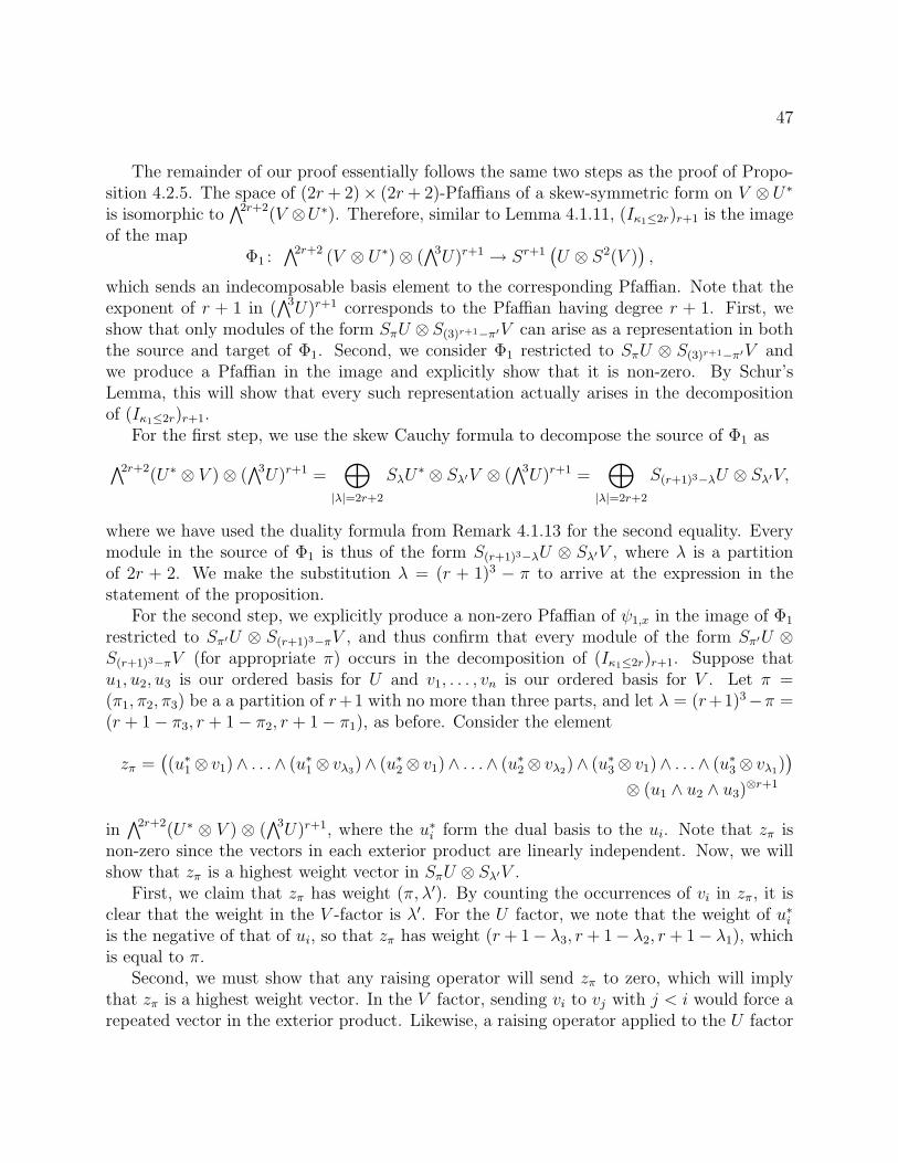
47

The remainder of our proof essentially follows the same two steps as the proof of Propo-sition 4.2.5. The space of (2r + 2)× (2r + 2)-Pfaffians of a skew-symmetric form on V ⊗ U∗is isomorphic to

∧2r+2(V ⊗U∗). Therefore, similar to Lemma 4.1.11, (Iκ1≤2r)r+1 is the imageof the map

Φ1 :∧2r+2 (V ⊗ U∗)⊗ (

∧3U)r+1 → Sr+1(U ⊗ S2(V )

),

which sends an indecomposable basis element to the corresponding Pfaffian. Note that theexponent of r + 1 in (

∧3U)r+1 corresponds to the Pfaffian having degree r + 1. First, weshow that only modules of the form SπU ⊗ S(3)r+1−π′V can arise as a representation in boththe source and target of Φ1. Second, we consider Φ1 restricted to SπU ⊗ S(3)r+1−π′V andwe produce a Pfaffian in the image and explicitly show that it is non-zero. By Schur’sLemma, this will show that every such representation actually arises in the decompositionof (Iκ1≤2r)r+1.

For the first step, we use the skew Cauchy formula to decompose the source of Φ1 as∧2r+2(U∗ ⊗ V )⊗ (∧3U)r+1 =

⊕|λ|=2r+2

SλU∗ ⊗ Sλ′V ⊗ (

∧3U)r+1 =⊕

|λ|=2r+2

S(r+1)3−λU ⊗ Sλ′V,

where we have used the duality formula from Remark 4.1.13 for the second equality. Everymodule in the source of Φ1 is thus of the form S(r+1)3−λU ⊗ Sλ′V , where λ is a partitionof 2r + 2. We make the substitution λ = (r + 1)3 − π to arrive at the expression in thestatement of the proposition.

For the second step, we explicitly produce a non-zero Pfaffian of ψ1,x in the image of Φ1

restricted to Sπ′U ⊗ S(r+1)3−πV , and thus confirm that every module of the form Sπ′U ⊗S(r+1)3−πV (for appropriate π) occurs in the decomposition of (Iκ1≤2r)r+1. Suppose thatu1, u2, u3 is our ordered basis for U and v1, . . . , vn is our ordered basis for V . Let π =(π1, π2, π3) be a a partition of r+1 with no more than three parts, and let λ = (r+1)3−π =(r + 1− π3, r + 1− π2, r + 1− π1), as before. Consider the element

zπ =((u∗1⊗ v1)∧ . . .∧ (u∗1⊗ vλ3)∧ (u∗2⊗ v1)∧ . . .∧ (u∗2⊗ vλ2)∧ (u∗3⊗ v1)∧ . . .∧ (u∗3⊗ vλ1)

)⊗ (u1 ∧ u2 ∧ u3)

⊗r+1

in∧2r+2(U∗ ⊗ V ) ⊗ (

∧3U)r+1, where the u∗i form the dual basis to the ui. Note that zπ isnon-zero since the vectors in each exterior product are linearly independent. Now, we willshow that zπ is a highest weight vector in SπU ⊗ Sλ′V .

First, we claim that zπ has weight (π, λ′). By counting the occurrences of vi in zπ, it isclear that the weight in the V -factor is λ′. For the U factor, we note that the weight of u∗iis the negative of that of ui, so that zπ has weight (r + 1− λ3, r + 1− λ2, r + 1− λ1), whichis equal to π.

Second, we must show that any raising operator will send zπ to zero, which will implythat zπ is a highest weight vector. In the V factor, sending vi to vj with j < i would force arepeated vector in the exterior product. Likewise, a raising operator applied to the U factor

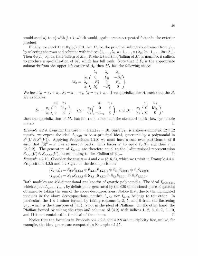
48

would send u∗i to u∗j with j > i, which would, again, create a repeated factor in the exteriorproduct.

Finally, we check that Φ1(zπ) 6= 0. Let Mπ be the principal submatrix obtained from ψ1,x

by selecting the rows and columns with indices 1, . . . , λ3, n+1, . . . , n+λ2, 2n+1, . . . , 2n+λ1.Then Φ1(zπ) equals the Pfaffian of Mπ. To check that the Pfaffian of Mπ is nonzero, it sufficesto produce a specialization of Mπ which has full rank. Note that if Bi is the appropriatesubmatrix from the upper-left corner of Ai, then Mπ has the following shape

Mπ =

λ3 λ2 λ1

λ3 0 B3 −B2

λ2 −Bt3 0 B1

λ1 Bt2 −Bt

1 0

.We have λ1 = π1 + π2, λ2 = π1 + π3, λ3 = π2 + π3. If we specialize the Ai such that the Bi

are as follows

B1 =

(π2 π1

π1 0 Idπ1

π3 0 0

), B2 =

( π2 π1

π3 0 0π2 −Idπ2 0

), and B3 =

(π1 π3

π3 0 Idπ3

π2 0 0

),

then the specialization of Mπ has full rank, since it is the standard block skew-symmetricmatrix.

Example 4.2.9. Consider the case n = 4 and c1 = 10. Since ψ1,x is a skew-symmetric 12× 12matrix, we expect the ideal Iκ1≤10 to be a principal ideal, generated by a polynomial inS6(U ⊗ S2(V )). Applying Proposition 4.2.8, we must have a sum over partitions π of 6such that (3)6 − π′ has at most 4 parts. This forces π′ to equal (3, 3), and thus π =(2, 2, 2). The generators of Iκ1≤10 are therefore equal to the 1-dimensional representationS2,2,2(U)⊗ S3,3,3,3(V ), corresponding to the Pfaffian of ψ1,x.

Example 4.2.10. Consider the case n = 4 and c = (3, 6, 3), which we revisit in Example 4.4.4.Propositions 4.2.5 and 4.2.8 give us the decompositions:

(Iκ0≤3)4 = S2,2S3,3,1,1 ⊕ S2,1,1S4,2,1,1 ⊕ S3,1S3,2,2,1 ⊕ S4S2,2,2,2,

(Iκ1≤6)4 = S2,2S3,3,1,1 ⊕ S2,1,1S3,3,2 ⊕ S3,1S3,2,2,1 ⊕ S4S2,2,2,2.

Both modules are 495-dimensional and consist of quartic polynomials. The ideal Iκ≤(3,6,3),which equals Iκ6≤6+Iκ0≤3 by definition, is generated by the 630-dimensional space of quarticsobtained by taking the sum of the above decompositions. Notice that, due to the highlightedmodules in the above decompositions, neither Iκ0≤3 nor Iκ1≤6 belongs to the other. Inparticular, the 4 × 4-minor formed by taking columns 1, 2, 5, and 9 from the flatteningψ0,x, which is the transpose of (4.1), is not in the ideal of Pfaffians. On the other hand, thePfaffian formed by taking the rows and columns of (4.2) with indices 1, 2, 5, 6, 7, 9, 10,and 11 is not contained in the ideal of the minors.

Notice that the formulas in Propositions 4.2.5 and 4.2.8 are multiplicity free, unlike, forexample, the ideal generators computed in Example 4.1.15.

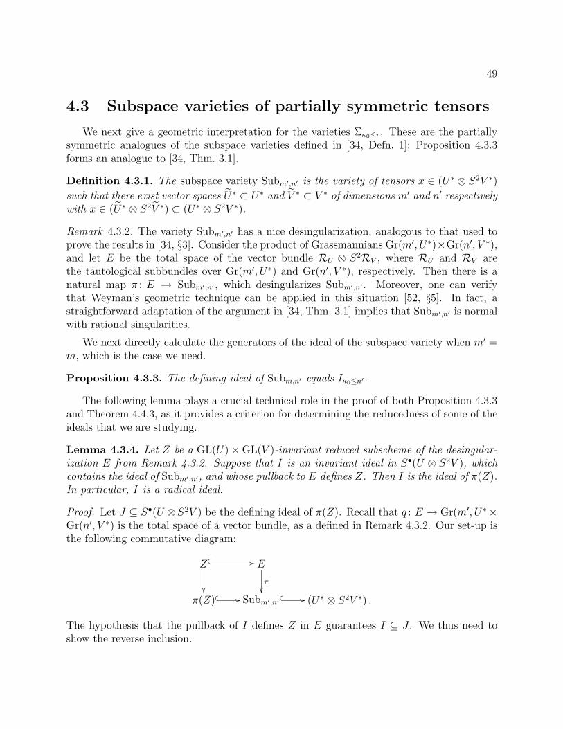
49

4.3 Subspace varieties of partially symmetric tensors

We next give a geometric interpretation for the varieties Σκ0≤r. These are the partiallysymmetric analogues of the subspace varieties defined in [34, Defn. 1]; Proposition 4.3.3forms an analogue to [34, Thm. 3.1].

Definition 4.3.1. The subspace variety Subm′,n′ is the variety of tensors x ∈ (U∗ ⊗ S2V ∗)

such that there exist vector spaces U∗ ⊂ U∗ and V ∗ ⊂ V ∗ of dimensions m′ and n′ respectivelywith x ∈ (U∗ ⊗ S2V ∗) ⊂ (U∗ ⊗ S2V ∗).

Remark 4.3.2. The variety Subm′,n′ has a nice desingularization, analogous to that used toprove the results in [34, §3]. Consider the product of Grassmannians Gr(m′, U∗)×Gr(n′, V ∗),and let E be the total space of the vector bundle RU ⊗ S2RV , where RU and RV arethe tautological subbundles over Gr(m′, U∗) and Gr(n′, V ∗), respectively. Then there is anatural map π : E → Subm′,n′ , which desingularizes Subm′,n′ . Moreover, one can verifythat Weyman’s geometric technique can be applied in this situation [52, §5]. In fact, astraightforward adaptation of the argument in [34, Thm. 3.1] implies that Subm′,n′ is normalwith rational singularities.

We next directly calculate the generators of the ideal of the subspace variety when m′ =m, which is the case we need.

Proposition 4.3.3. The defining ideal of Subm,n′ equals Iκ0≤n′.

The following lemma plays a crucial technical role in the proof of both Proposition 4.3.3and Theorem 4.4.3, as it provides a criterion for determining the reducedness of some of theideals that we are studying.

Lemma 4.3.4. Let Z be a GL(U)×GL(V )-invariant reduced subscheme of the desingular-ization E from Remark 4.3.2. Suppose that I is an invariant ideal in S•(U ⊗ S2V ), whichcontains the ideal of Subm′,n′, and whose pullback to E defines Z. Then I is the ideal of π(Z).In particular, I is a radical ideal.

Proof. Let J ⊆ S•(U ⊗S2V ) be the defining ideal of π(Z). Recall that q : E → Gr(m′, U∗×Gr(n′, V ∗) is the total space of a vector bundle, as a defined in Remark 4.3.2. Our set-up isthe following commutative diagram:

Z //

E

π

π(Z) // Subm′,n′ // (U∗ ⊗ S2V ∗) .

The hypothesis that the pullback of I defines Z in E guarantees I ⊆ J . We thus need toshow the reverse inclusion.

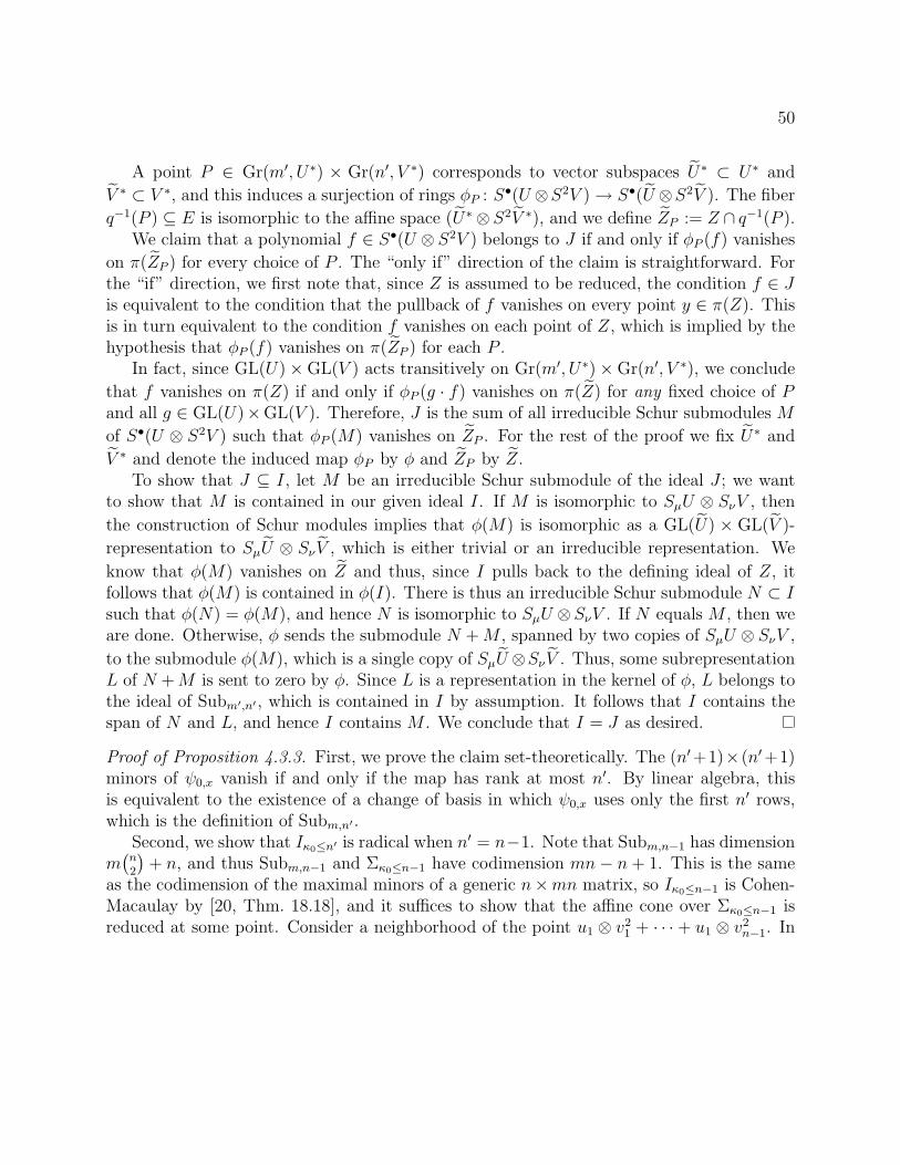
50

A point P ∈ Gr(m′, U∗) × Gr(n′, V ∗) corresponds to vector subspaces U∗ ⊂ U∗ and

V ∗ ⊂ V ∗, and this induces a surjection of rings φP : S•(U ⊗S2V )→ S•(U ⊗S2V ). The fiber

q−1(P ) ⊆ E is isomorphic to the affine space (U∗⊗ S2V ∗), and we define ZP := Z ∩ q−1(P ).We claim that a polynomial f ∈ S•(U ⊗ S2V ) belongs to J if and only if φP (f) vanishes

on π(ZP ) for every choice of P . The “only if” direction of the claim is straightforward. Forthe “if” direction, we first note that, since Z is assumed to be reduced, the condition f ∈ Jis equivalent to the condition that the pullback of f vanishes on every point y ∈ π(Z). Thisis in turn equivalent to the condition f vanishes on each point of Z, which is implied by thehypothesis that φP (f) vanishes on π(ZP ) for each P .

In fact, since GL(U)×GL(V ) acts transitively on Gr(m′, U∗)×Gr(n′, V ∗), we conclude

that f vanishes on π(Z) if and only if φP (g · f) vanishes on π(Z) for any fixed choice of Pand all g ∈ GL(U)×GL(V ). Therefore, J is the sum of all irreducible Schur submodules M

of S•(U ⊗ S2V ) such that φP (M) vanishes on ZP . For the rest of the proof we fix U∗ and

V ∗ and denote the induced map φP by φ and ZP by Z.To show that J ⊆ I, let M be an irreducible Schur submodule of the ideal J ; we want

to show that M is contained in our given ideal I. If M is isomorphic to SµU ⊗ SνV , then

the construction of Schur modules implies that φ(M) is isomorphic as a GL(U) × GL(V )-

representation to SµU ⊗ SνV , which is either trivial or an irreducible representation. We

know that φ(M) vanishes on Z and thus, since I pulls back to the defining ideal of Z, itfollows that φ(M) is contained in φ(I). There is thus an irreducible Schur submodule N ⊂ Isuch that φ(N) = φ(M), and hence N is isomorphic to SµU ⊗SνV . If N equals M , then weare done. Otherwise, φ sends the submodule N +M , spanned by two copies of SµU ⊗ SνV ,

to the submodule φ(M), which is a single copy of SµU ⊗SνV . Thus, some subrepresentationL of N +M is sent to zero by φ. Since L is a representation in the kernel of φ, L belongs tothe ideal of Subm′,n′ , which is contained in I by assumption. It follows that I contains thespan of N and L, and hence I contains M . We conclude that I = J as desired.

Proof of Proposition 4.3.3. First, we prove the claim set-theoretically. The (n′+1)×(n′+1)minors of ψ0,x vanish if and only if the map has rank at most n′. By linear algebra, thisis equivalent to the existence of a change of basis in which ψ0,x uses only the first n′ rows,which is the definition of Subm,n′ .

Second, we show that Iκ0≤n′ is radical when n′ = n−1. Note that Subm,n−1 has dimensionm(n2

)+ n, and thus Subm,n−1 and Σκ0≤n−1 have codimension mn− n + 1. This is the same

as the codimension of the maximal minors of a generic n×mn matrix, so Iκ0≤n−1 is Cohen-Macaulay by [20, Thm. 18.18], and it suffices to show that the affine cone over Σκ0≤n−1 isreduced at some point. Consider a neighborhood of the point u1 ⊗ v2

1 + · · · + u1 ⊗ v2n−1. In

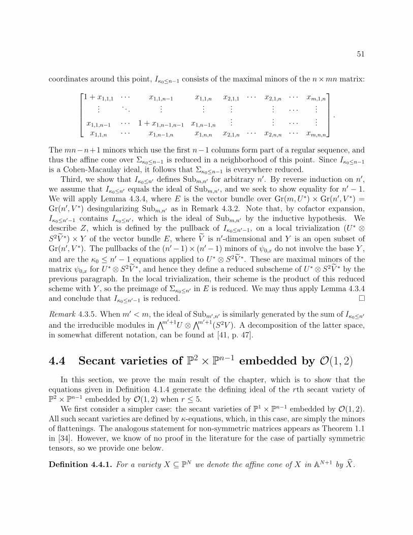
51

coordinates around this point, Iκ0≤n−1 consists of the maximal minors of the n×mn matrix:1 + x1,1,1 · · · x1,1,n−1 x1,1,n x2,1,1 · · · x2,1,n · · · xm,1,n

.... . .

......

...... · · · ...

x1,1,n−1 · · · 1 + x1,n−1,n−1 x1,n−1,n...

... · · · ...x1,1,n · · · x1,n−1,n x1,n,n x2,1,n · · · x2,n,n · · · xm,n,n

.The mn−n+1 minors which use the first n−1 columns form part of a regular sequence, andthus the affine cone over Σκ0≤n−1 is reduced in a neighborhood of this point. Since Iκ0≤n−1

is a Cohen-Macaulay ideal, it follows that Σκ0≤n−1 is everywhere reduced.Third, we show that Iκ0≤n′ defines Subm,n′ for arbitrary n′. By reverse induction on n′,

we assume that Iκ0≤n′ equals the ideal of Subm,n′ , and we seek to show equality for n′ − 1.We will apply Lemma 4.3.4, where E is the vector bundle over Gr(m,U∗) × Gr(n′, V ∗) =Gr(n′, V ∗) desingularizing Subm,n′ as in Remark 4.3.2. Note that, by cofactor expansion,Iκ0≤n′−1 contains Iκ0≤n′ , which is the ideal of Subm,n′ by the inductive hypothesis. Wedescribe Z, which is defined by the pullback of Iκ0≤n′−1, on a local trivialization (U∗ ⊗S2V ∗) × Y of the vector bundle E, where V is n′-dimensional and Y is an open subset ofGr(n′, V ∗). The pullbacks of the (n′− 1)× (n′− 1) minors of ψ0,x do not involve the base Y ,

and are the κ0 ≤ n′ − 1 equations applied to U∗ ⊗ S2V ∗. These are maximal minors of thematrix ψ0,x for U∗⊗ S2V ∗, and hence they define a reduced subscheme of U∗⊗ S2V ∗ by theprevious paragraph. In the local trivialization, their scheme is the product of this reducedscheme with Y , so the preimage of Σκ0≤n′ in E is reduced. We may thus apply Lemma 4.3.4and conclude that Iκ0≤n′−1 is reduced.

Remark 4.3.5. When m′ < m, the ideal of Subm′,n′ is similarly generated by the sum of Iκ0≤n′

and the irreducible modules in∧m′+1U ⊗

∧m′+1(S2V ). A decomposition of the latter space,in somewhat different notation, can be found at [41, p. 47].

4.4 Secant varieties of P2 × Pn−1 embedded by O(1, 2)

In this section, we prove the main result of the chapter, which is to show that theequations given in Definition 4.1.4 generate the defining ideal of the rth secant variety ofP2 × Pn−1 embedded by O(1, 2) when r ≤ 5.

We first consider a simpler case: the secant varieties of P1 × Pn−1 embedded by O(1, 2).All such secant varieties are defined by κ-equations, which, in this case, are simply the minorsof flattenings. The analogous statement for non-symmetric matrices appears as Theorem 1.1in [34]. However, we know of no proof in the literature for the case of partially symmetrictensors, so we provide one below.

Definition 4.4.1. For a variety X ⊆ PN we denote the affine cone of X in AN+1 by X.

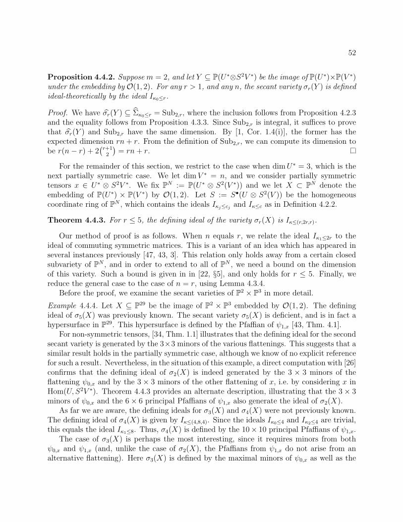
52

Proposition 4.4.2. Suppose m = 2, and let Y ⊆ P(U∗⊗S2V ∗) be the image of P(U∗)×P(V ∗)under the embedding by O(1, 2). For any r > 1, and any n, the secant variety σr(Y ) is definedideal-theoretically by the ideal Iκ0≤r.

Proof. We have σr(Y ) ⊆ Σκ0≤r = Sub2,r, where the inclusion follows from Proposition 4.2.3and the equality follows from Proposition 4.3.3. Since Sub2,r is integral, it suffices to provethat σr(Y ) and Sub2,r have the same dimension. By [1, Cor. 1.4(i)], the former has theexpected dimension rn+ r. From the definition of Sub2,r, we can compute its dimension tobe r(n− r) + 2

(r+12

)= rn+ r.

For the remainder of this section, we restrict to the case when dimU∗ = 3, which is thenext partially symmetric case. We let dimV ∗ = n, and we consider partially symmetrictensors x ∈ U∗ ⊗ S2V ∗. We fix PN := P(U∗ ⊗ S2(V ∗)) and we let X ⊂ PN denote theembedding of P(U∗) × P(V ∗) by O(1, 2). Let S := S•(U ⊗ S2(V )) be the homogeneouscoordinate ring of PN , which contains the ideals Iκj≤cj and Iκ≤c as in Definition 4.2.2.

Theorem 4.4.3. For r ≤ 5, the defining ideal of the variety σr(X) is Iκ≤(r,2r,r).

Our method of proof is as follows. When n equals r, we relate the ideal Iκ1≤2r to theideal of commuting symmetric matrices. This is a variant of an idea which has appeared inseveral instances previously [47, 43, 3]. This relation only holds away from a certain closedsubvariety of PN , and in order to extend to all of PN , we need a bound on the dimensionof this variety. Such a bound is given in in [22, §5], and only holds for r ≤ 5. Finally, wereduce the general case to the case of n = r, using Lemma 4.3.4.

Before the proof, we examine the secant varieties of P2 × P3 in more detail.

Example 4.4.4. Let X ⊆ P29 be the image of P2 × P3 embedded by O(1, 2). The definingideal of σ5(X) was previously known. The secant variety σ5(X) is deficient, and is in fact ahypersurface in P29. This hypersurface is defined by the Pfaffian of ψ1,x [43, Thm. 4.1].

For non-symmetric tensors, [34, Thm. 1.1] illustrates that the defining ideal for the secondsecant variety is generated by the 3×3 minors of the various flattenings. This suggests that asimilar result holds in the partially symmetric case, although we know of no explicit referencefor such a result. Nevertheless, in the situation of this example, a direct computation with [26]confirms that the defining ideal of σ2(X) is indeed generated by the 3 × 3 minors of theflattening ψ0,x and by the 3× 3 minors of the other flattening of x, i.e. by considering x inHom(U, S2V ∗). Theorem 4.4.3 provides an alternate description, illustrating that the 3× 3minors of ψ0,x and the 6× 6 principal Pfaffians of ψ1,x also generate the ideal of σ2(X).

As far we are aware, the defining ideals for σ3(X) and σ4(X) were not previously known.The defining ideal of σ4(X) is given by Iκ≤(4,8,4). Since the ideals Iκ0≤4 and Iκ2≤4 are trivial,this equals the ideal Iκ1≤8. Thus, σ4(X) is defined by the 10× 10 principal Pfaffians of ψ1,x.

The case of σ3(X) is perhaps the most interesting, since it requires minors from bothψ0,x and ψ1,x (and, unlike the case of σ2(X), the Pfaffians from ψ1,x do not arise from analternative flattening). Here σ3(X) is defined by the maximal minors of ψ0,x as well as the

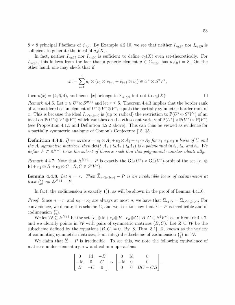
53

8 × 8 principal Pfaffians of ψ1,x. By Example 4.2.10, we see that neither Iκ0≤3 nor Iκ1≤6 issufficient to generate the ideal of σ3(X).

In fact, neither Iκ0≤3 nor Iκ1≤6 is sufficient to define σ3(X) even set-theoretically. ForIκ0≤3, this follows from the fact that a generic element y ∈ Σκ0≤3 has κ1(y) = 8. On theother hand, one may check that if

x :=3∑i=1

ui ⊗ (v1 ⊗ vi+1 + vi+1 ⊗ v1) ∈ U∗ ⊗ S2V ∗,

then κ(x) = (4, 6, 4), and hence [x] belongs to Σκ1≤6 but not to σ3(X).

Remark 4.4.5. Let x ∈ U∗⊗S2V ∗ and let r ≤ 5. Theorem 4.4.3 implies that the border rankof x, considered as an element of U∗⊗V ∗⊗V ∗, equals the partially symmetric border rank ofx. This is because the ideal Iκ≤(r,2r,r) is (up to radical) the restriction to P(U∗⊗S2V ∗) of anideal on P(U∗⊗V ∗⊗V ∗) which vanishes on the rth secant variety of P(U∗)×P(V ∗)×P(V ∗)(see Proposition 4.1.5 and Definition 4.2.2 above). This can thus be viewed as evidence fora partially symmetric analogue of Comon’s Conjecture [15, §5].

Definition 4.4.6. If we write x = e1⊗A1 + e2⊗A2 + e3⊗A3 for e1, e2, e3 a basis of U andthe Ai symmetric matrices, then det(t1A1 +t2A2 +t3A3) is a polynomial in t1, t2, and t3. Wedefine P ⊂ AN+1 to be the subset of those x such that this polynomial vanishes identically.

Remark 4.4.7. Note that AN+1 − P is exactly the GL(U∗) × GL(V ∗)-orbit of the set e1 ⊗Id + e2 ⊗B + e3 ⊗ C | B,C ∈ S2V ∗.

Lemma 4.4.8. Let n = r. Then Σκ≤(r,2r,r) − P is an irreducible locus of codimension atleast

(r2

)on AN+1 − P .

In fact, the codimension is exactly(r2

), as will be shown in the proof of Lemma 4.4.10.

Proof. Since n = r, and κ0 = κ2 are always at most n, we have that Σκ1≤r = Σκ≤(r,2r,r). For

convenience, we denote this scheme Σ, and we seek to show that Σ−P is irreducible and ofcodimension

(r2

).

We letW ⊆ AN+1 be the set e1⊗Id+e2⊗B+e3⊗C | B,C ∈ S2V ∗ as in Remark 4.4.7,and we identify points in W with pairs of symmetric matrices (B,C). Let Z ⊆ W be thesubscheme defined by the equations [B,C] = 0. By [8, Thm. 3.1], Z, known as the varietyof commuting symmetric matrices, is an integral subscheme of codimension

(r2

)in W .

We claim that Σ − P is irreducible. To see this, we note the following equivalence ofmatrices under elementary row and column operations: 0 Id −B

−Id 0 CB −C 0

∼ 0 Id 0−Id 0 0

0 0 BC − CB

.

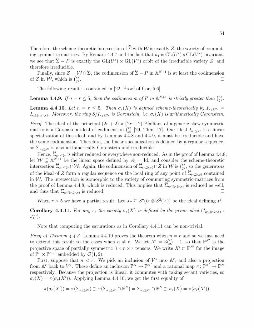
54

Therefore, the scheme-theoretic intersection of Σ withW is exactly Z, the variety of commut-ing symmetric matrices. By Remark 4.4.7 and the fact that κ1 is GL(U∗)×GL(V ∗)-invariant,

we see that Σ − P is exactly the GL(U∗) × GL(V ∗) orbit of the irreducible variety Z, andtherefore irreducible.

Finally, since Z =W ∩ Σ, the codimension of Σ−P in AN+1 is at least the codimensionof Z in W , which is

(r2

).

The following result is contained in [22, Proof of Cor. 5.6].

Lemma 4.4.9. If n = r ≤ 5, then the codimension of P in AN+1 is strictly greater than(n2

).

Lemma 4.4.10. Let n = r ≤ 5. Then σr(X) is defined scheme-theoretically by Iκ1≤2r =Iκ≤(r,2r,r). Moreover, the ring S/Iκ1≤2r is Gorenstein, i.e. σr(X) is arithmetically Gorenstein.

Proof. The ideal of the principal (2r + 2) × (2r + 2)-Pfaffians of a generic skew-symmetricmatrix is a Gorenstein ideal of codimension

(r2

)[29, Thm. 17]. Our ideal Iκ1≤2r is a linear

specialization of this ideal, and by Lemmas 4.4.8 and 4.4.9, it must be irreducible and havethe same codimension. Therefore, the linear specialization is defined by a regular sequence,so Σκ1≤2r is also arithmetically Gorenstein and irreducible.

Hence, Σκ1≤2r is either reduced or everywhere non-reduced. As in the proof of Lemma 4.4.8,let W ⊆ AN+1 be the linear space defined by A1 = Id, and consider the scheme-theoreticintersection Σκ1≤2r∩W . Again, the codimension of Σ(r,2r,r)∩Z inW is

(r2

), so the generators

of the ideal of Z form a regular sequence on the local ring of any point of Σ(r,2r,r) containedin W . The intersection is isomorphic to the variety of commuting symmetric matrices fromthe proof of Lemma 4.4.8, which is reduced. This implies that Σκ≤(r,2r,r) is reduced as well,and thus that Σκ≤(r,2r,r) is reduced.

When r > 5 we have a partial result. Let JP ⊆ S•(U ⊗ S2(V )) be the ideal defining P .

Corollary 4.4.11. For any r, the variety σr(X) is defined by the prime ideal (Iκ≤(r,2r,r) :J∞P ).

Note that computing the saturations as in Corollary 4.4.11 can be non-trivial.

Proof of Theorem 4.4.3. Lemma 4.4.10 proves the theorem when n = r and so we just needto extend this result to the cases when n 6= r. We let N ′ = 3

(r2

)− 1, so that PN ′ is the

projective space of partially symmetric 3× r × r tensors. We write X ′ ⊂ PN ′ for the imageof P2 × Pr−1 embedded by O(1, 2).

First, suppose that n < r. We pick an inclusion of V ∗ into Ar, and also a projectionfrom Ar back to V ∗. These define an inclusion PN → PN ′ and a rational map π : PN ′ → PNrespectively. Because the projection is linear, it commutes with taking secant varieties, soσr(X) = π(σr(X

′)). Applying Lemma 4.4.10, we get the first equality of

π(σr(X′)) = π(Σκ1≤2r) ⊃ π(Σκ1≤2r ∩ PN) = Σκ1≤2r ∩ PN ⊃ σr(X) = π(σr(X

′)).

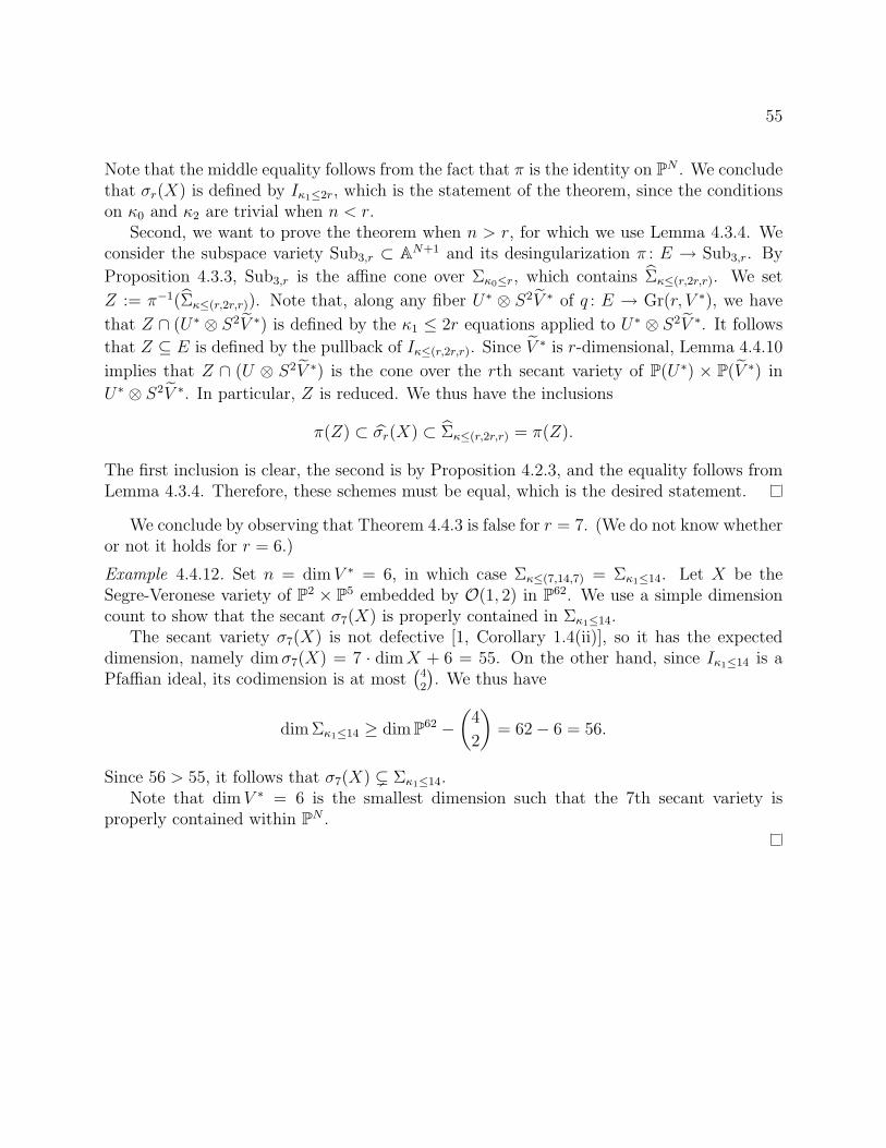
55

Note that the middle equality follows from the fact that π is the identity on PN . We concludethat σr(X) is defined by Iκ1≤2r, which is the statement of the theorem, since the conditionson κ0 and κ2 are trivial when n < r.

Second, we want to prove the theorem when n > r, for which we use Lemma 4.3.4. Weconsider the subspace variety Sub3,r ⊂ AN+1 and its desingularization π : E → Sub3,r. By

Proposition 4.3.3, Sub3,r is the affine cone over Σκ0≤r, which contains Σκ≤(r,2r,r). We set

Z := π−1(Σκ≤(r,2r,r)). Note that, along any fiber U∗ ⊗ S2V ∗ of q : E → Gr(r, V ∗), we have

that Z ∩ (U∗ ⊗ S2V ∗) is defined by the κ1 ≤ 2r equations applied to U∗ ⊗ S2V ∗. It follows

that Z ⊆ E is defined by the pullback of Iκ≤(r,2r,r). Since V ∗ is r-dimensional, Lemma 4.4.10

implies that Z ∩ (U ⊗ S2V ∗) is the cone over the rth secant variety of P(U∗) × P(V ∗) in

U∗ ⊗ S2V ∗. In particular, Z is reduced. We thus have the inclusions

π(Z) ⊂ σr(X) ⊂ Σκ≤(r,2r,r) = π(Z).

The first inclusion is clear, the second is by Proposition 4.2.3, and the equality follows fromLemma 4.3.4. Therefore, these schemes must be equal, which is the desired statement.

We conclude by observing that Theorem 4.4.3 is false for r = 7. (We do not know whetheror not it holds for r = 6.)

Example 4.4.12. Set n = dimV ∗ = 6, in which case Σκ≤(7,14,7) = Σκ1≤14. Let X be theSegre-Veronese variety of P2 × P5 embedded by O(1, 2) in P62. We use a simple dimensioncount to show that the secant σ7(X) is properly contained in Σκ1≤14.

The secant variety σ7(X) is not defective [1, Corollary 1.4(ii)], so it has the expecteddimension, namely dimσ7(X) = 7 · dimX + 6 = 55. On the other hand, since Iκ1≤14 is aPfaffian ideal, its codimension is at most

(42

). We thus have

dim Σκ1≤14 ≥ dim P62 −(

4

2

)= 62− 6 = 56.

Since 56 > 55, it follows that σ7(X) ( Σκ1≤14.Note that dimV ∗ = 6 is the smallest dimension such that the 7th secant variety is

properly contained within PN .

56

Chapter 5

How are SNPs distributed in genes?

In this chapter, we use the equations from Chapter 4 to study the distribution of singlenucleotide polymorphisms (SNPs) within the human genes. The occurrence of SNPs isshaped by the functional constraints imposed by the fact that they code for amino acidswithin proteins. As we will see, the equations of secant varieties will allow us to detect theseconstraints from the data.

5.1 Testing mixture models

In this section, we introduce the notion of a mixture model for a m× n× n contingencytable, and develop a statistical test for membership in such a model. For more about mixturemodels and secant varieties in algebraic statistics, see Chapter 4 of [19]. First, we define aprobabilistic model for producing triples of integers from the product [m]× [n]× [n].

Definition 5.1.1. A mixture model with r hidden states is described by a probability dis-tribution ph on the hidden states 1, . . . , r, together with, for each h ≤ r, a probabilitydistribution uhi on [m] and a probability distribution vhj on [n]. The triples are produced byfirst choosing an integer h with probability ph and then choosing i, j, and k independentlywith probabilities uhi, vij, and vik respectively. The three integers i, j, and k are output.

From this description, it follows immediately that the probability of a given triple is

P (i, j, k) =r∑

h=1

phuhivhjvkj. (5.1)

We can incorporate the quantity ph into the values of uhi, in which case this equationbecomes the expression for the (i, j, k)-entry of a semi-symmetric tensor in the rth secantvariety of the Segre-Veronese variety. As in Chapter 4, we will represent a probabilitydistribution on [3]× [n]× [n] by a triple of symmetric matrices A, B, and C, which contain

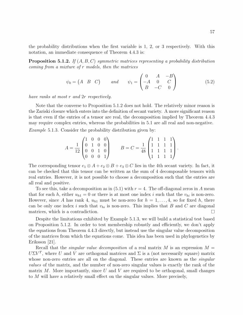
57

the probability distributions when the first variable is 1, 2, or 3 respectively. With thisnotation, an immediate consequence of Theorem 4.4.3 is:

Proposition 5.1.2. If (A,B,C) symmetric matrices representing a probability distributioncoming from a mixture of r models, then the matrices

ψ0 =(A B C

)and ψ1 =

0 A −B−A 0 CB −C 0

(5.2)

have ranks at most r and 2r respectively.

Note that the converse to Proposition 5.1.2 does not hold. The relatively minor reason isthe Zariski closure which enters into the definition of secant variety. A more significant reasonis that even if the entries of a tensor are real, the decomposition implied by Theorem 4.4.3may require complex entries, whereas the probabilities in 5.1 are all real and non-negative.

Example 5.1.3. Consider the probability distribution given by:

A =1

12

1 0 0 00 1 0 00 0 1 00 0 0 1

B = C =1

48

1 1 1 11 1 1 11 1 1 11 1 1 1

.

The corresponding tensor e1 ⊗A+ e2 ⊗B + e3 ⊗C lies in the 4th secant variety. In fact, itcan be checked that this tensor can be written as the sum of 4 decomposable tensors withreal entries. However, it is not possible to choose a decomposition such that the entries areall real and positive.

To see this, take a decomposition as in (5.1) with r = 4. The off-diagonal zeros in A meanthat for each h, either uh1 = 0 or there is at most one index i such that the vhi is non-zero.However, since A has rank 4, uh1 must be non-zero for h = 1, . . . , 4, so for fixed h, therecan be only one index i such that vhi is non-zero. This implies that B and C are diagonalmatrices, which is a contradiction.

Despite the limitations exhibited by Example 5.1.3, we will build a statistical test basedon Proposition 5.1.2. In order to test membership robustly and efficiently, we don’t applythe equations from Theorem 4.4.3 directly, but instead use the singular value decompositionof the matrices from which the equations come. This idea has been used in phylogenetics byEriksson [21].

Recall that the singular value decomposition of a real matrix M is an expression M =UΣV T , where U and V are orthogonal matrices and Σ is a (not necessarily square) matrixwhose non-zero entries are all on the diagonal. These entries are known as the singularvalues of the matrix, and the number of non-zero singular values is exactly the rank of thematrix M . More importantly, since U and V are required to be orthogonal, small changesto M will have a relatively small effect on the singular values. More precisely,

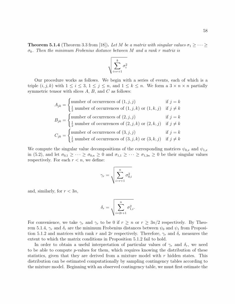
58

Theorem 5.1.4 (Theorem 3.3 from [18]). Let M be a matrix with singular values σ1 ≥ · · · ≥σk. Then the minimum Frobenius distance between M and a rank r matrix is√√√√ k∑

i=r+1

σ2i

Our procedure works as follows. We begin with a series of events, each of which is atriple (i, j, k) with 1 ≤ i ≤ 3, 1 ≤ j ≤ n, and 1 ≤ k ≤ n. We form a 3 × n × n partiallysymmetric tensor with slices A, B, and C as follows:

Ajk =

number of occurrences of (1, j, j) if j = k12

number of occurrences of (1, j, k) or (1, k, j) if j 6= k

Bjk =

number of occurrences of (2, j, j) if j = k12

number of occurrences of (2, j, k) or (2, k, j) if j 6= k

Cjk =

number of occurrences of (3, j, j) if j = k12

number of occurrences of (3, j, k) or (3, k, j) if j 6= k

We compute the singular value decompositions of the corresponding matrices ψ0,x and ψ1,x

in (5.2), and let σ0,1 ≥ · · · ≥ σ0,n ≥ 0 and σ1,1 ≥ · · · ≥ σ1,3n ≥ 0 be their singular valuesrespectively. For each r < n, we define:

γr =

√√√√ n∑i=r+1

σ20,i

and, similarly, for r < 3n,

δr =

√√√√ n∑i=2r+1

σ21,i.

For convenience, we take γr and γr to be 0 if r ≥ n or r ≥ 3n/2 respectively. By Theo-rem 5.1.4, γr and δr are the minimum Frobenius distances between ψ0 and ψ1 from Proposi-tion 5.1.2 and matrices with rank r and 2r respectively. Therefore, γr and δr measures theextent to which the matrix conditions in Proposition 5.1.2 fail to hold.

In order to obtain a useful interpretation of particular values of γr and δr, we needto be able to compute p-values for them, which requires knowing the distribution of thesestatistics, given that they are derived from a mixture model with r hidden states. Thisdistribution can be estimated computationally by sampling contingency tables according tothe mixture model. Beginning with an observed contingency table, we must first estimate the

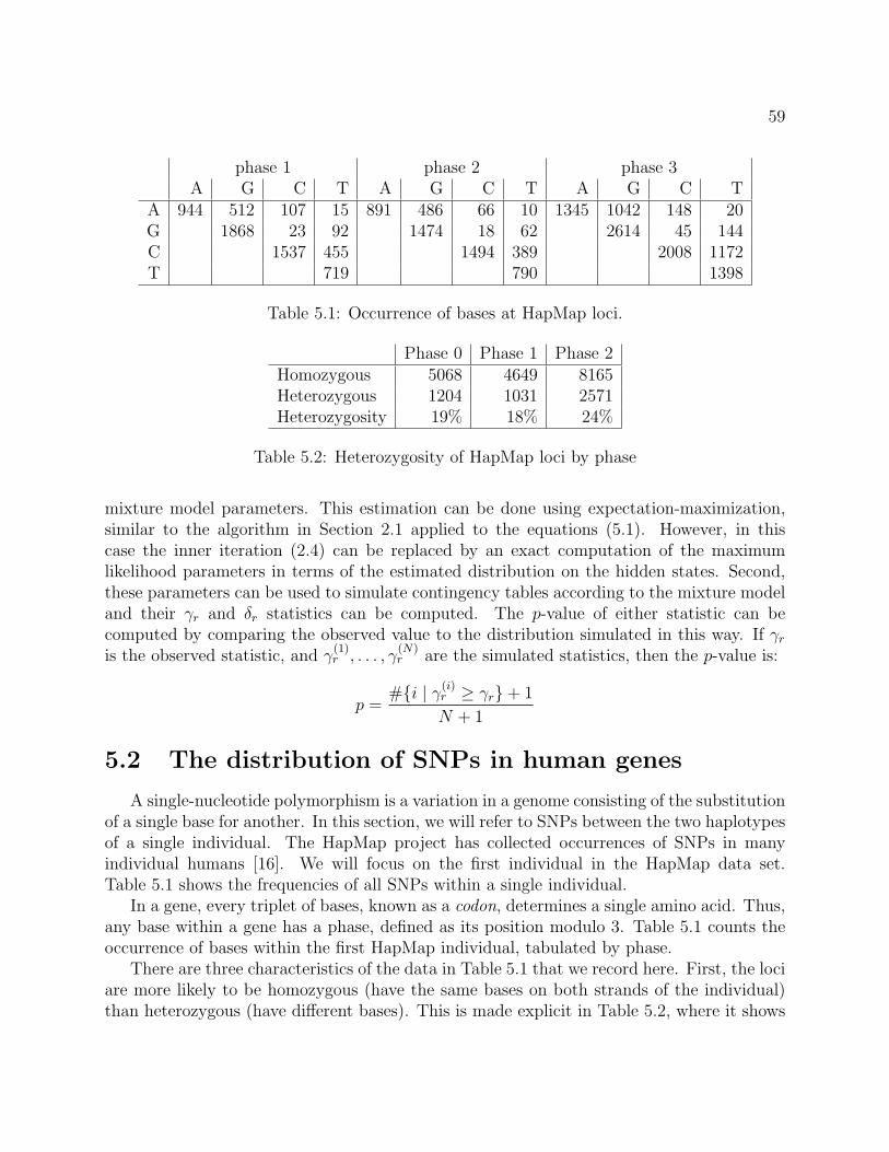
59

phase 1 phase 2 phase 3A G C T A G C T A G C T

A 944 512 107 15 891 486 66 10 1345 1042 148 20G 1868 23 92 1474 18 62 2614 45 144C 1537 455 1494 389 2008 1172T 719 790 1398

Table 5.1: Occurrence of bases at HapMap loci.

Phase 0 Phase 1 Phase 2Homozygous 5068 4649 8165Heterozygous 1204 1031 2571Heterozygosity 19% 18% 24%

Table 5.2: Heterozygosity of HapMap loci by phase

mixture model parameters. This estimation can be done using expectation-maximization,similar to the algorithm in Section 2.1 applied to the equations (5.1). However, in thiscase the inner iteration (2.4) can be replaced by an exact computation of the maximumlikelihood parameters in terms of the estimated distribution on the hidden states. Second,these parameters can be used to simulate contingency tables according to the mixture modeland their γr and δr statistics can be computed. The p-value of either statistic can becomputed by comparing the observed value to the distribution simulated in this way. If γris the observed statistic, and γ

(1)r , . . . , γ

(N)r are the simulated statistics, then the p-value is:

p =#i | γ(i)

r ≥ γr+ 1

N + 1

5.2 The distribution of SNPs in human genes

A single-nucleotide polymorphism is a variation in a genome consisting of the substitutionof a single base for another. In this section, we will refer to SNPs between the two haplotypesof a single individual. The HapMap project has collected occurrences of SNPs in manyindividual humans [16]. We will focus on the first individual in the HapMap data set.Table 5.1 shows the frequencies of all SNPs within a single individual.

In a gene, every triplet of bases, known as a codon, determines a single amino acid. Thus,any base within a gene has a phase, defined as its position modulo 3. Table 5.1 counts theoccurrence of bases within the first HapMap individual, tabulated by phase.

There are three characteristics of the data in Table 5.1 that we record here. First, the lociare more likely to be homozygous (have the same bases on both strands of the individual)than heterozygous (have different bases). This is made explicit in Table 5.2, where it shows

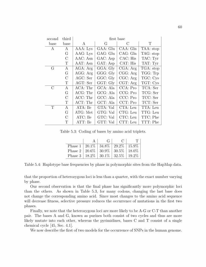
60

second third first basebase base A G C T

A A AAA: Lys GAA: Glu CAA: Gln TAA: stopG AAG: Lys GAG: Glu CAG: Gln TAG: stopC AAC: Asn GAC: Asp CAC: His TAC: TyrT AAT: Asn GAT: Asp CAT: His TAT: Tyr

G A AGA: Arg GGA: Gly CGA: Arg TGA: stopG AGG: Arg GGG: Gly CGG: Arg TGG: TrpC AGC: Ser GGC: Gly CGC: Arg TGC: CysT AGT: Ser GGT: Gly CGT: Arg TGT: Cys

C A ACA: Thr GCA: Ala CCA: Pro TCA: SerG ACG: Thr GCG: Ala CCG: Pro TCG: SerC ACC: Thr GCC: Ala CCC: Pro TCC: SerT ACT: Thr GCT: Ala CCT: Pro TCT: Ser

T A ATA: Ile GTA: Val CTA: Leu TTA: LeuG ATG: Met GTG: Val CTG: Leu TTG: LeuC ATC: Ile GTC: Val CTC: Leu TTC: PheT ATT: Ile GTT: Val CTT: Leu TTT: Phe

Table 5.3: Coding of bases by amino acid triplets.

A G C TPhase 1 20.1% 34.8% 29.2% 15.9%Phase 2 20.6% 30.9% 30.5% 18.0%Phase 3 18.2% 30.1% 32.5% 19.2%

Table 5.4: Haplotype base frequencies by phase in polymorphic sites from the HapMap data.

that the proportion of heterozygous loci is less than a quarter, with the exact number varyingby phase.

Our second observation is that the final phase has significantly more polymorphic locithan the others. As shown in Table 5.3, for many codons, changing the last base doesnot change the corresponding amino acid. Since most changes to the amino acid sequencewill decrease fitness, selective pressure reduces the occurrence of mutations in the first twophases.

Finally, we note that the heterozygous loci are more likely to be A-G or C-T than anotherpair. The bases A and G, known as purines both consist of two cycles and thus are morelikely mutate into each other, whereas the pyrimidines, bases C and T consist of a singlechemical cycle [45, Sec. 4.1].

We now describe the first of two models for the occurrence of SNPs in the human genome.

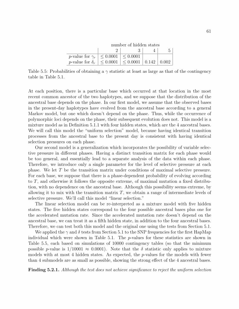
61

number of hidden states2 3 4 5

p-value for γr ≤ 0.0001 ≤ 0.0001p-value for δr ≤ 0.0001 ≤ 0.0001 0.142 0.002

Table 5.5: Probabilities of obtaining a γ statistic at least as large as that of the contingencytable in Table 5.1.

At each position, there is a particular base which occurred at that location in the mostrecent common ancestor of the two haplotypes, and we suppose that the distribution of theancestral base depends on the phase. In our first model, we assume that the observed basesin the present-day haplotypes have evolved from the ancestral base according to a generalMarkov model, but one which doesn’t depend on the phase. Thus, while the occurrence ofpolymorphic loci depends on the phase, their subsequent evolution does not. This model is amixture model as in Definition 5.1.1 with four hidden states, which are the 4 ancestral bases.We will call this model the “uniform selection” model, because having identical transitionprocesses from the ancestral base to the present day is consistent with having identicalselection pressures on each phase.

Our second model is a generalization which incorporates the possibility of variable selec-tive pressure in different phases. Having a distinct transition matrix for each phase wouldbe too general, and essentially lead to a separate analysis of the data within each phase.Therefore, we introduce only a single parameter for the level of selective pressure at eachphase. We let T be the transition matrix under conditions of maximal selective pressure.For each base, we suppose that there is a phase-dependent probability of evolving accordingto T , and otherwise it follows the opposite extreme, of maximal mutation a fixed distribu-tion, with no dependence on the ancestral base. Although this possibility seems extreme, byallowing it to mix with the transition matrix T , we obtain a range of intermediate levels ofselective pressure. We’ll call this model “linear selection.”

The linear selection model can be re-interpreted as a mixture model with five hiddenstates. The five hidden states correspond to the four possible ancestral bases plus one forthe accelerated mutation rate. Since the accelerated mutation rate doesn’t depend on theancestral base, we can treat it as a fifth hidden state, in addition to the four ancestral bases.Therefore, we can test both this model and the original one using the tests from Section 5.1.

We applied the γ and δ tests from Section 5.1 to the SNP frequencies for the first HapMapindividual which were shown in Table 5.1. The p-values for these statistics are shown inTable 5.5, each based on simulations of 10000 contingency tables (so that the minimumpossible p-value is 1/10001 ≈ 0.0001). Note that the δ statistic only applies to mixturemodels with at most 4 hidden states. As expected, the p-values for the models with fewerthan 4 submodels are as small as possible, showing the strong effect of the 4 ancestral bases.

Finding 5.2.1. Although the test does not achieve significance to reject the uniform selection

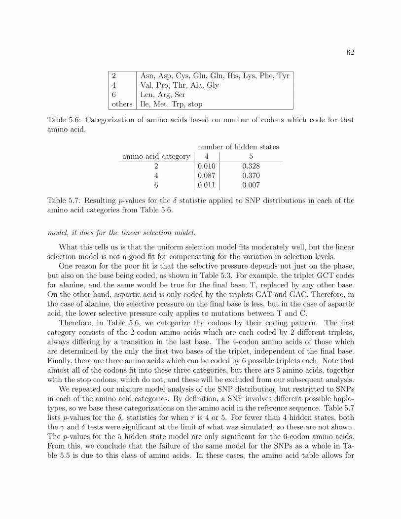
62

2 Asn, Asp, Cys, Glu, Gln, His, Lys, Phe, Tyr4 Val, Pro, Thr, Ala, Gly6 Leu, Arg, Serothers Ile, Met, Trp, stop

Table 5.6: Categorization of amino acids based on number of codons which code for thatamino acid.

number of hidden statesamino acid category 4 5

2 0.010 0.3284 0.087 0.3706 0.011 0.007

Table 5.7: Resulting p-values for the δ statistic applied to SNP distributions in each of theamino acid categories from Table 5.6.

model, it does for the linear selection model.

What this tells us is that the uniform selection model fits moderately well, but the linearselection model is not a good fit for compensating for the variation in selection levels.

One reason for the poor fit is that the selective pressure depends not just on the phase,but also on the base being coded, as shown in Table 5.3. For example, the triplet GCT codesfor alanine, and the same would be true for the final base, T, replaced by any other base.On the other hand, aspartic acid is only coded by the triplets GAT and GAC. Therefore, inthe case of alanine, the selective pressure on the final base is less, but in the case of asparticacid, the lower selective pressure only applies to mutations between T and C.

Therefore, in Table 5.6, we categorize the codons by their coding pattern. The firstcategory consists of the 2-codon amino acids which are each coded by 2 different triplets,always differing by a transition in the last base. The 4-codon amino acids of those whichare determined by the only the first two bases of the triplet, independent of the final base.Finally, there are three amino acids which can be coded by 6 possible triplets each. Note thatalmost all of the codons fit into these three categories, but there are 3 amino acids, togetherwith the stop codons, which do not, and these will be excluded from our subsequent analysis.

We repeated our mixture model analysis of the SNP distribution, but restricted to SNPsin each of the amino acid categories. By definition, a SNP involves different possible haplo-types, so we base these categorizations on the amino acid in the reference sequence. Table 5.7lists p-values for the δr statistics for when r is 4 or 5. For fewer than 4 hidden states, boththe γ and δ tests were significant at the limit of what was simulated, so these are not shown.The p-values for the 5 hidden state model are only significant for the 6-codon amino acids.From this, we conclude that the failure of the same model for the SNPs as a whole in Ta-ble 5.5 is due to this class of amino acids. In these cases, the amino acid table allows for

63

extra mutations in the final phase, but there is some selective pressure for transitions overtransversions in the second phase. On the other hand, for the 2- and 4-codon amino acids,the linear selection model is sufficient.

We have shown that, as expected, the selective pressures on SNPs depend on the phasewithin the codon. However, this dependence is not as simple as having a higher level ofpolymorphism in the final phase. Instead, the existence of 6-codon amino acids means thatthe selective pressures vary quantitatively as well as quantitatively. On the other hand, foramino acids with simpler coding patterns, the SNPs can be effectively modeled by a simplephase-dependent increase in the mutation rate.

We conclude that the study of tensors can be brought to bear on the analysis of genomicdata. We hope that further developments will lead to more applications of tensors andalgebraic statistics to computational biology.

64

Bibliography

[1] Hirotachi Abo and Maria Chiara Brambilla. Secant varieties of Segre-Veronese varietiesPm × Pn embedded by O(1, 2). Experiment. Math., 18(3):369–384, 2009.

[2] Dan Bates and Frank Sottile. Khovanskii-Rolle continuation for real solutions.arXiv:0908.4579, 2009.

[3] Shuchao Bi. Tensor rank, simultaneous diagonalization, and some related matrix vari-eties. preprint, 2010.

[4] K. Birnbaum, J. W. Jung, J. Y. Wang, G. M. Lambert, J. A. Hirst, D. W. Galbraith,and P. N. Benfey. Cell type-specific expression profiling in plants via cell sorting ofprotoplasts from fluorescent reporter lines. Nature Methods, 2(8):615, 2005.

[5] K. Birnbaum, D. E. Shasha, J. Y. Wang, J. W. Jung, G. M. Lambert, D. W. Galbraith,and P. N. Benfey. A gene expression map of the Arabidopsis root. Science’s STKE,302(5652):1956, 2003.

[6] M. Bonke, S. Thitamadee, A. P. Mahonen, M. T. Wauser, and Y. Helariutta. APLregulates vascular tissue identity in Arabidopsis. Nature(London), 426(6963):181–186,2003.

[7] Siobhan M. Brady, David A. Orlando, J. Y. Lee, J. Y. Wang, J. Koch, J. R. Dinneny,D. Mace, U. Ohler, and Philip N. Benfey. A high-resolution root spatiotemporal mapreveals dominant expression patterns. Science, 318(5851):801–806, 2007.

[8] J. P. Brennan, M. V. Pinto, and W. V. Vasconcelos. The Jacobian module of a Liealgebra. Trans. Amer. Math. Soc., 321(1):183–196, 1990.

[9] W. Busch and J. U. Lohmann. Profiling a plant: expression analysis in Arabidopsis.Current Opinion in Plant Biology, 10(2):136–141, 2007.

[10] Dustin Cartwright. An algorithm for finding postive solutions to polynomial equations.preprint, 2010.

65

[11] Dustin Cartwright, Daniel Erman, and Luke Oeding. Secant varieties of P2 × Pn em-bedded by O(1, 2). preprint, 2010.

[12] Dustin A. Cartwright, Siobhan M. Brady, David A. Orlando, Bernd Sturmfels, andPhilip N. Benfey. Reconstruction spatiotemporal gene expression data from partialobservations. Bioinformatics, 25(19):2581–2587, 2009.

[13] Dustin A. Cartwright, Daniel Erman, Mauricio Velasco, and Bianca Viray. Hilbertschemes of 8 points. Algebra & Number Theory, 3(7):763–795, 2009.

[14] B. Chaudhuri, F. Hormann, S. Lalonde, S. M. Brady, D. A. Orlando, P. N. Benfey, andW. B. Frommer. Protonophore- and pH-insensitive glucose and sucrose accumulationdetected by FRET nanosensors in Arabidopsis root tips. Plant J., 56(6):948–962, 2008.

[15] Pierre Comon, Gene Golub, Lek-Heng Lim, and Bernard Mourrain. Symmetric tensorsand symmetric tensor rank. SIAM J. Matrix Anal. Appl., 30(3):1254–1279, 2008.

[16] The International HapMap Consortium. A second generation human haplotype map ofover 3.1 million snps. Nature, 449:851–861, 2007.

[17] J. N. Darroch and D. Ratcliff. Generalized iterative scaling for log-linear models. Annalsof Math. Stat., 43(5):1470–1480, 1972.

[18] James W. Demmel. Applied Numerical Linear Algebra. Society for Industrial andApplied Mathematics (SIAM), 1997.

[19] Mathias Drton, Bernd Sturmfels, and Seth Sullivant. Lectures on Algebraic Statistics,volume 39 of Oberwolfach Seminars. Birkhauser, 2009.

[20] David Eisenbud. Commutative Algebra with a View Toward Algebraic Geometry, volume150 of Graduate Texts in Mathematics. Springer, 2004.

[21] Nicholas Eriksson. Tree construction using singular value decomposition. In AlgebraicStatistics for Computational Biology, pages 347–358. Cambridge University Press, 2005.

[22] Daniel Erman and Mauricio Velasco. A syzygetic approach to the smoothability ofzero-dimensional schemes. Adv. in Math., 224:1143–1166, 2010.

[23] William Fulton and Joe Harris. Representation theory, volume 129 of Graduate Textsin Mathematics. Springer-Verlag, New York, 1991. A first course, Readings in Mathe-matics.

[24] Luis David Garcia, Michael Stillman, and Bernd Sturmfels. Algebraic geometry ofBayesian networks. J. Symbolic Comput., 39(3-4):331–355, 2005.

66

[25] Debashis Ghosh. Mixture models for assessing differential expression in complex tissuesusing microarray data. Bioinformatics, 20:1663–1669, 2004.

[26] Daniel R. Grayson and Michael E. Stillman. Macaulay 2, a software system for researchin algebraic geometry. Available at http://www.math.uiuc.edu/Macaulay2/.

[27] Anjali S. Iyer-Pascuzzi and Philip N. Benfey. Transcriptional networks in root cell fatespecification. Biochim. Biophys. Acta., 1789(4):315–25, April 2009.

[28] Yuling Jiao, S Lori Tausta, Neeru Gandotra, Ning Sun, Tie Liu, Nicole K Clay, TeresaCeserani, Meiqin Chen, Ligeng Ma, Matthew Holford, Hui yong Zhang, Hongyu Zhao,Xing-Wang Deng, and Timothy Nelson. A transcriptome atlas of rice cell types uncoverscellular, functional, and developmental hierarchies. Nature Genetics, 41:258–263, 2009.

[29] H. Kleppe and D. Laksov. The algebraic structure and deformation of Pfaffian schemes.J. Algebra, 64(1):167–189, 1980.

[30] J. M. Landsberg and Laurent Manivel. On the ideals of secant varieties of Segre varieties.Found. Comput. Math., 4(4):397–422, 2004.

[31] J. M. Landsberg and Laurent Manivel. Generalizations of Strassen’s equations for secantvarieties of Segre varieties. Comm. Algebra, 36(2):405–422, 2008.

[32] J. M. Landsberg and G. Ottaviani. Equations for secant varieties to Veronese varieties.arXiv:1006.0180, 2010.

[33] J. M. Landsberg and Zach Teitler. On the ranks and border ranks of symmetric tensors.Found. Comput. Math., 10(3):339–366, 2010.

[34] J. M. Landsberg and Jerzy Weyman. On the ideals and singularities of secant varietiesof Segre varieties. Bull. Lond. Math. Soc., 39(4):685–697, 2007.

[35] J. M. Landsberg and Jerzy Weyman. On secant varieties of compact Hermitian sym-metric spaces. J. Pure Appl. Algebra, 213(11):2075–2086, 2009.

[36] Jean B. Lasserre, Monique Laurent, and Philipp Rostalski. Semidefinite characterizationand computation of real radical ideals. Foundations of Computational Mathematics,8(5):607–647, 2008.

[37] Jean B. Lasserre, Monique Laurent, and Philipp Rostalski. A prolongation-projectionalgorithm for computing the finite real variety of an ideal. Theoretical Computer Science,410(27–29):2685–2700, 2009.

[38] Daniel D. Lee and H. Sebastian Seung. Algorithms for non-negative matrix factorization.Adv. Neural Info. Proc. Syst., 13:556–562, 2001.

67

[39] J.Y. Lee, J. Colinas, J.Y. Wang, D. Mace, U. Ohler, and P.N. Benfey. Transcrip-tional and posttranscriptional regulation of transcription factor expression in Arabidop-sis roots. Proceedings of the National Academy of Sciences, 103(15):6055–6060, 2006.

[40] M. Levine and E.H. Davidson. Gene regulatory networks for development. Proc NatlAcad Sci USA, 102(14):4936–42, 2005.

[41] I. G. Macdonald. Symmetric functions and Hall polynomials. Oxford MathematicalMonographs. The Clarendon Press Oxford University Press, New York, second edition,1995. With contributions by A. Zelevinsky, Oxford Science Publications.

[42] A.P. Mahonen, M. Bonke, L. Kauppinen, M. Riikonen, P.N. Benfey, and Y. Helari-utta. A novel two-component hybrid molecule regulates vascular morphogenesis of theArabidopsis root. Genes & Development, 14(23):2938–2943, 2000.

[43] Giorgio Ottaviani. Symplectic bundles on the plane, secant varieties and Luroth quarticsrevisited. In Vector bundles and low codimensional subvarieties: state of the art andrecent developments, volume 21 of Quad. Mat., pages 315–352. Dept. Math., SecondaUniv. Napoli, Caserta, 2007.

[44] Giorgio Ottaviani. An invariant regarding Waring’s problem for cubic polynomials.Nagoya Math. J., 193:95–110, 2009.

[45] Lior Pachter and Bernd Sturmfels. Algebraic Statistics for Computational Biology. Cam-bridge University Press, 2005.

[46] A. Slapak and A. Yeredor. Near-optimal weighting in characteristic-function basedICA. In 18th European Signal Processing Conference (EUSIPCO-2010), pages 890–894,August 23-27 2010.

[47] Volker Strassen. Rank and optimal computation of generic tensors. Linear AlgebraAppl., 52/53:645–685, 1983.

[48] Emil Toeplitz. Uber ein Flachennetz zweiter Ordnung. Math. Ann., 11:434–463, 1877.

[49] M. A. A. van Leeuwen, A. M. Coehn, and B. Lisser. LiE, A Package for Lie GroupComputations. Computer Algebra Nederland, 1992.

[50] D. Venet, F. Pecasse, C. Maenhaut, and H. Bersini. Separation of samples into theirconstituents using gene expression data. Bioinformatics, 17:S279–S287, 2001.

[51] Jan Verschelde. PHCPACK: A general-purpose solver for polynomial systems by ho-motopy continuation.

[52] Jerzy Weyman. Cohomology of Vector Bundles and Syzygies, volume 149 of CambridgeTracts in Mathematics. Cambridge University Press, Cambridge, 2003.