Applications of geometric optimisation techniques to

Applications of geometricoptimisation techniques to

engineering problemsJochen Trumpf

[email protected]

Department of Information Engineering

Research School of Information Sciences and Engineering

The Australian National University

and

National ICT Australia Ltd.

Applications of geometric optimisation techniques to engineering problems – p. 1/31

overview

What is geometric optimisation?


overview


Ex 1: Blind Source Separation (BSS)


overview



Independent Component Analysis (ICA)


overview




Ex 2: face recognition


overview





dominant eigenspaces of matrix pencils (LDA)


overview






Ex 3: time series clustering


overview







“on-the-fly” geometry


overview







“on-the-fly” geometry

state of the art and open problems


What is geometricoptimisation?

Given a real valued function

f : M −→ R, x 7→ f(x)

defined on some geometric object M , here asmooth manifold, find a method to compute (if itexists)

x∗ := argminx∈M

f(x)

that utilises the (local) geometry of M .


Ex 1: Blind SourceSeparation

The cocktail party problem.

Image: http://www.lnt.de/LMS/research/projects/BSS


Ex 1: Blind SourceSeparation

source signals observed mixtures

audio, EEG, MEG, fMRI, wireless, ...

Image: http://www.cis.hut.fi/aapo/papers/NCS99web/nod e17.html


BSS – the modelIndividual signals ( i = 1, . . . , d)

xi : [0, T ] −→ R, t 7→ xi(t)

are being uniformly sampled and the samplescollected into row vectors

xi =(

xi(t0) xi(t0 + ∆) . . . xi(t0 + (N − 1) · ∆))

which are then stacked into a matrix

X =

x1...

xd

∈ R

d×N .


BSS – the model

It is assumed that there are as many sourcesignals as observed signals and that they arerelated by

Xo = M · Xs

where Xo, Xs ∈ Rd×N and M ∈ GLd(R).


BSS – the model

It is assumed that there are as many sourcesignals as observed signals and that they arerelated by

Xo = M · Xs

where Xo, Xs ∈ Rd×N and M ∈ GLd(R).

Task: Find Xs (or M−1) from knowing Xo

subject to some plausible criterion.


BSS as ICA problem

We treat the columns of Xo as i.i.d. samples of anobserved random variable vector Y given by

Y = M · X

where X is the unknown random variable sourcevector.


BSS as ICA problem

We treat the columns of Xo as i.i.d. samples of anobserved random variable vector Y given by

Y = M · X

where X is the unknown random variable sourcevector.

The ICA paradigm is now that the components ofX, i.e. the individual signals, are mutuallyindependent.


BSS as ICA problem

Hence, we are trying to find the invertible M thatmakes the components of the corresponding X“as independent as possible”.


BSS as ICA problem

Hence, we are trying to find the invertible M thatmakes the components of the corresponding X“as independent as possible”.

Note: The matrix M in

Y = M · X

is identifiable up to scaling and permutations ifand only if the components of X are mutuallyindependent and at most one of them isGaussian.


BSS as ICA problem

A computational trick is centering andprewhitening: multiply by the square root of thecovariance matrix of Y (assuming finite secondmoments) to obtain

Y = Q · X

where Q ∈ Od(R) and X and Y are zero mean andunit variance.


BSS as ICA problem

A computational trick is centering andprewhitening: multiply by the square root of thecovariance matrix of Y (assuming finite secondmoments) to obtain

Y = Q · X

where Q ∈ Od(R) and X and Y are zero mean andunit variance.

Note: Prewhitening from samples works best inthe Gaussian case ...

see IEEE TSP, 53(10):3625–3632, 2005


ICA as geometricoptimisation problem

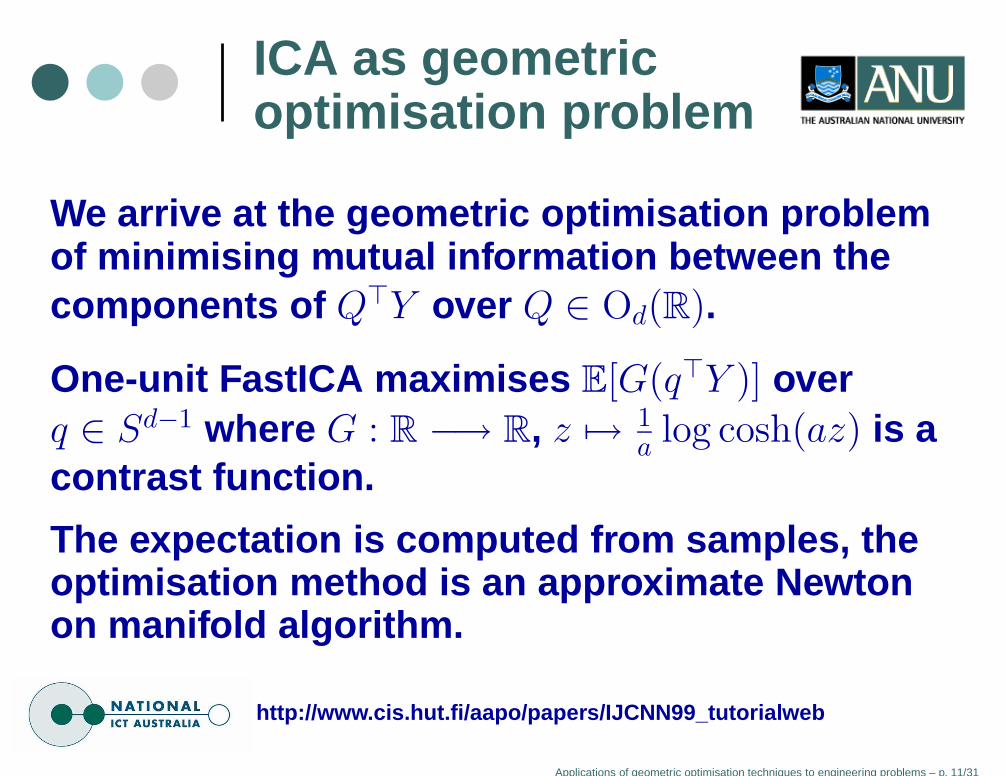
We arrive at the geometric optimisation problemof minimising mutual information between thecomponents of Q⊤Y over Q ∈ Od(R).


ICA as geometricoptimisation problem

We arrive at the geometric optimisation problemof minimising mutual information between thecomponents of Q⊤Y over Q ∈ Od(R).

One-unit FastICA maximises E[G(q⊤Y )] overq ∈ Sd−1 where G : R −→ R, z 7→ 1

alog cosh(az) is a

contrast function.

The expectation is computed from samples, theoptimisation method is an approximate Newtonon manifold algorithm.

http://www.cis.hut.fi/aapo/papers/IJCNN99_tutorialwe b



Image: IEEE TPAMI, 23(2):228–233, 2001


face recognition – themodel

An image is represented as a vector X ∈ Rt.

Images are divided in c classes with Nj imagesX

ji , i = 1, . . . , Nj in class j = 1, . . . , c.


face recognition – themodel

An image is represented as a vector X ∈ Rt.

Images are divided in c classes with Nj imagesX

ji , i = 1, . . . , Nj in class j = 1, . . . , c.

Consider the within-class scatter matrix

Sw =∑

i,j

(Xji − µj)(X

ji − µj)

⊤

and the between-class scatter matrix

Sb =∑

j

(µj − µ)(µj − µ)⊤.


face recognition asLDA problem

Orthogonally projecting the image vectors into alower dimensional space Y = Q⊤X yieldsprojected scatter matrices Q⊤S{w,b}Q.




The aim is to maximise det(Q⊤SbQ)det(Q⊤SwQ) over Q ∈ St(d, t),

the orthogonal Stiefel manifold.




The aim is to maximise det(Q⊤SbQ)det(Q⊤SwQ) over Q ∈ St(d, t),

the orthogonal Stiefel manifold.

This amounts to finding the dominantd-dimensional eigenspace of the pencil (Sb, Sw).


LDA as geometricoptimisation problem

Given a symmetric/positive-definite matrix pencil(A,B) with eigenvalues ( Ax = λBx)λ1 ≥ · · · ≥ λd > λd+1 ≥ · · · ≥ λn the uniqued-dimensional dominant eigenspace is theunique global maximum of

f : Grass(d, n) −→ R, [Q] 7→ tr(Q⊤AQ(QTBQ)−1)

see J Comp and Appl Math, 189(1):274–285, 2006


Ex 3: time-seriesclustering

A time series is a (finite) sequence {xt}t=1,...,N ofvectors (in R

n), e.g. arising from (sampling) atrajectory of a dynamical system.A popular method of time-series clustering worksin delay space

xp

xp−1...

xp−l+1

∣∣∣∣∣∣∣∣∣∣∣∣

p = l, . . . , N}



Knowl. Inf. Syst., 8(2):154-177, 2005



ICDM 2005, pp. 114–121


state of the art

Let M be a d-dimensional Riemannian manifoldand let f : M → R be smooth.

The derivative of f at x ∈ M is a linear form

D f(x) : TxM → R

A point x∗ ∈ M is called a critical point of f if

D f(x∗)ξ = 0, ∀ξ ∈ Tx∗M.


state of the artFact: x∗ ∈ M is a strict local minimum of f if

(a) x∗ is a critical point of f ,

(b) the Hessian form

hess f(x∗) : Tx∗M× Tx∗M → R

is positive definite.


state of the artFact: x∗ ∈ M is a strict local minimum of f if

(a) x∗ is a critical point of f ,

(b) the Hessian form

hess f(x∗) : Tx∗M× Tx∗M → R

is positive definite.

Geodesics of M: ∀x ∈ M and ξ ∈ TxM

γx : R ∋ (−ε, ε) → M, ε 7→ γx(ε)

such that γx(0) = x and γ̇x(0) = ξ.


state of the art

Riemannian Newton direction ξ ∈ TxM by solving

hess f(x) · ξ = grad f(x)

-r

xk r xk+1

M

/PPPPPP��PPPPPP ξ


state of the art

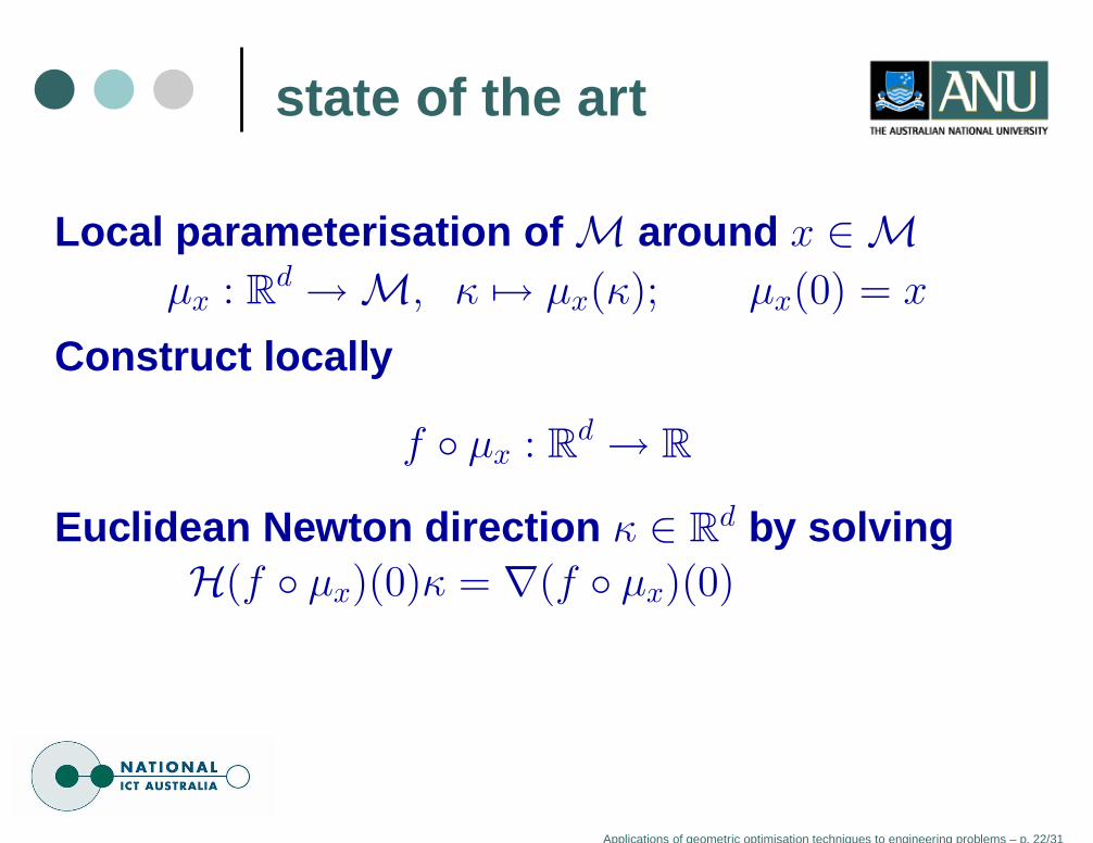
Local parameterisation of M around x ∈ M

µx : Rd → M, κ 7→ µx(κ); µx(0) = x

Construct locally

f ◦ µx : Rd → R

Euclidean Newton direction κ ∈ Rd by solving

H(f ◦ µx)(0)κ = ∇(f ◦ µx)(0)


state of the art

r

xkr

xk+1

M

κµ−1

x

νx

Rd

0 -

6

ZZZ~

rz

y


state of the artLet x∗ ∈ M be a nondegenerate critical point. Let{µx}x∈M and {νx}x∈M be locally smooth aroundx∗. Consider the following iteration on M

x0 ∈ M, xk+1 = νxk

(

Nf◦µxk(0)

)

(N)

Theorem: (Hüper-T.) Under the condition

Dµx∗(0) = D νx∗(0)

there exists an open neighborhood V ⊂ M of x∗

such that the point sequence generated by (N)converges quadratically to x∗ provided x0 ∈ V .


state of the art

know how to construct computable families ofcoordinate charts for St, Grass

can deal with approximate Newton

local convergence theory for more generaliterations (Manton-T.)

some global convergence results of trustregion on manifold schemes (Absil et al.)


trust-region methods

Image: http://www.inma.ucl.ac.be/˜blondel/workshops/ 2004/Absil.pdf


state of the art – ICA

One-unit ICA problem as an optimisation problemon Sd−1

f : Sd−1 → R, q 7→ E[G(q⊤Y )].

Geodesics, gradient, Hessian (Hüper-Shen)

γq : R → Sd−1, ε 7→ exp(

ε(ξq⊤− qξ⊤))

q.

grad f(q) =(

I − qq⊤)

E[G′(q⊤Y )Y ]

hess f(q) · ξ =(

E[G′′(q⊤Y )Y Y ⊤]︸︷︷︸

∈Rd×d

−E[G′(q⊤Y )q⊤Y ]︸︷︷︸

∈R

I)

· ξ



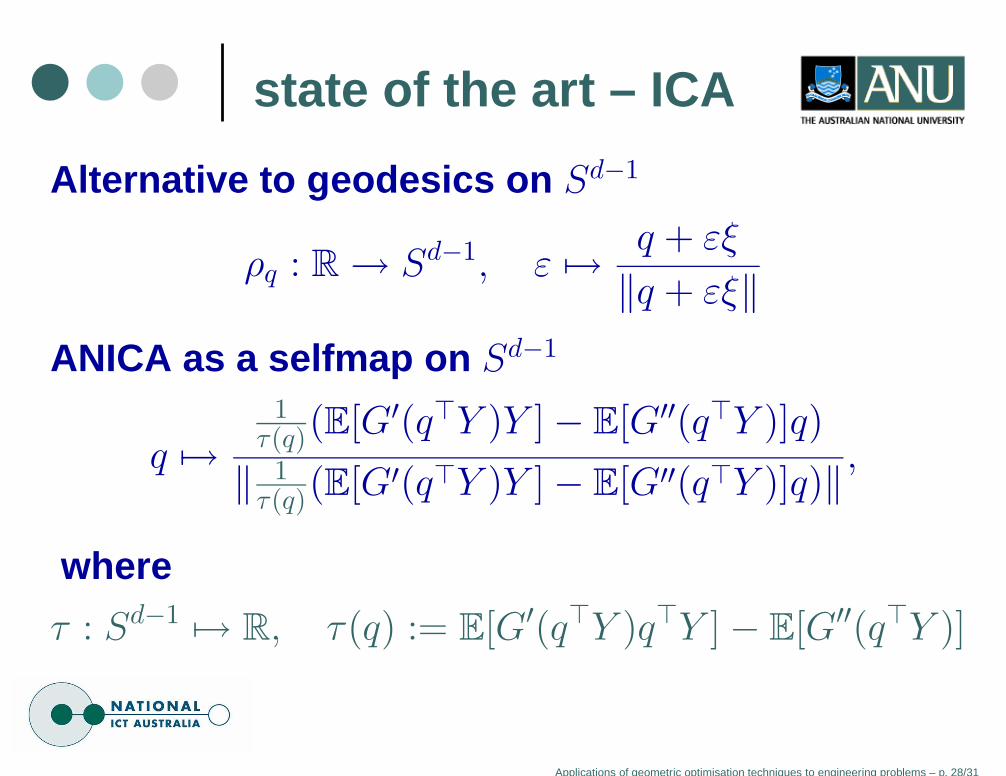
Alternative to geodesics on Sd−1

ρq : R → Sd−1, ε 7→q + εξ

‖q + εξ‖

ANICA as a selfmap on Sd−1

q 7→

1τ(q)(E[G′(q⊤Y )Y ] − E[G′′(q⊤Y )]q)

‖ 1τ(q)(E[G′(q⊤Y )Y ] − E[G′′(q⊤Y )]q)‖

,

where

τ : Sd−1 7→ R, τ(q) := E[G′(q⊤Y )q⊤Y ] − E[G′′(q⊤Y )]


state of the art – ICAFastICA vs ANICA

1 2 3 4 5 6 7 8

10−10

10−5

100

Iteration (k)

|| x(

k)−

x*

||

FastICAANICA


state of the art – ICAFastICA vs ANICA

1 2 3 4 5 6 7 8

10−10

10−5

100

Iteration (k)

|| x(

k)−

x*

||

FastICAANICA

Parallel version (ANLICA, Hüper-Shen) with costfunction

f : Od(R) → R, Q 7→m∑

i=1

E[G(q⊤i Y )]



0 10 20 30 40 50 6010

−7

10−6

10−5

10−4

10−3

10−2

10−1

100

101

Sweep

Nor

m (

x(i)

− x

(i)*

)

123456789

1 2 3 4 5 6 7 810

−16

10−14

10−12

10−10

10−8

10−6

10−4

10−2

100

102

Sweep

Nor

m (

x(i)

− x

(i)*

)

123456789

Parallel FastICA ANLICA


the end

Thank you.


Applications of geometric optimisation techniques to

Documents

Transcript of Applications of geometric optimisation techniques to