PROCEEDINGS, Thirty-Ninth Workshop on Geothermal Reservoir Engineering

Stanford University, Stanford, California, February 24-26, 2014

SGP-TR-202

1

Applications of Experimental Design and Response Surface Method in Probabilistic

Geothermal Resource Assessment – Preliminary Results

Jaime J. Quinao* and Sadiq J. Zarrouk

Department of Engineering Science, University of Auckland, Private Bag 92019, Auckland 1142, New Zealand

*jaime.quinao@mightyriver.co.nz

Keywords: Experimental design, response surface method, proxy models, uncertainty analysis, probabilistic resource assessment,

reservoir simulation,

ABSTRACT

Resource estimates in geothermal green-fields involve significant inherent uncertainty due to poorly constrained subsurface

parameters and multiple potential development scenarios. There is also limited published information on probabilistic resource

assessments of geothermal prospects. This paper explores the applications of a systematic experimental design (ED) and response

surface method (RSM) approach to generate probabilistic resource results.

ED and RSM have been successfully used in uncertainty analysis and resource evaluation of petroleum fields. These techniques

have also been used in a number of field management strategy assessments of geothermal brown-fields. This work presents the

preliminary results of a study to extend the geothermal applications of ED and RSM to geothermal green-field resource

assessments.

ED and RSM are applied to a simple geothermal process model and used to estimate the amount of electrical generating capacity

from this synthetic geothermal system. A response variable (electrical generating capacity) as a function of the main uncertain

parameters was derived from the simulation runs. This response function serves as the proxy model in Monte-Carlo probabilistic

analysis. For this preliminary study, distributions used for the main uncertain parameters are assumed. The probabilistic results

from the proxy model are compared with the probabilistic results from the mass in-place volumetric reserves method.

The results provide a preliminary understanding of the potential strengths and weaknesses of the ED and RSM methodologies as

applied to geothermal resource assessment. Future work will focus on refining the appropriate workflow, understanding the

distribution of uncertain parameters, and exploring the ED and RSM levels of complexity applicable to an actual green-field

numerical model.

1. INTRODUCTION

Probabilistic assessment of undeveloped geothermal resources has been necessary to accommodate the uncertainties in both the

subsurface parameters and the development scenario to be implemented. The geothermal industry has done this mainly through

Monte Carlo simulations of the parameters in the volumetric stored heat or mass in-place estimation methodologies (Grant and

Mahon, 1995; Parini et al., 1995; Parini and Riedel, 2000; Sanyal and Sarmiento, 2005; Williams et al., 2008; AGRCC, 2010; Garg

and Combs, 2010; Onur et al., 2010). The Monte Carlo simulation is applied to the parameters of the volumetric stored heat

equation where the parameters are allowed to vary over a range of values and within a defined probability distribution

(AGRCC, 2010). The range of parameter values ideally covers the range of uncertainty for that particular variable. This is strongly

influenced by the geothermal experts doing the estimate as shown by the review of geothermal resource estimation methodology

by Zarrouk and Simiyu (2013).

An example of a power capacity estimate based on volumetric stored heat equation is shown below (Zarrouk and Simiyu, 2013):

(1)

where is the power capacity in MWe, is the theoretical available heat in both the reservoir rock and fluid, is the recovery

factor that represents the fraction of recoverable heat from the system, is the conversion efficiency, is the project life, and is

the power plant load factor. The theoretical available heat, , is described by the following expression (AGRCC, 2010):

[( ) ( ) { ( ) ( )}] (2)

where the product of area and height, Ah, is the resource volume, is the porosity representing the fluid-filled fraction of the

volume, is the density of the rock, is the heat capacity of the rock, is the difference between the initial and final rock

temperature, and are the initial steam and liquid densities, and are the steam and liquid saturations, and are the

change in steam and liquid enthalpies.

The probabilistic resource assessment would be a Monte Carlo simulation of equation (1) where the parameters are randomly

sampled within their defined probability distribution range. The result is a probability density function (PDF) or a cumulative

distribution function of the power capacity (AGRCC, 2010). In this assessment, the most debated parameter is the recovery factor,

.

Quinao and Zarrouk

2

Parini and Riedel (2000) investigated the recovery factor using numerical simulation. In their approach, was based on the ratio

of total steam produced in 30 years to the original reservoir mass in-place. The use of numerical simulation to investigate the

relationship between the physics of the reservoir and the recovery factor is an improved probabilistic assessment based on the

volumetric method (equation 1).

The use of numerical simulation models for probabilistic resource assessment has never been a popular option due to the resources

required to build reservoir models and the perceived weakness of a model without production history calibration. However, use of

numerical simulations for the final resource assessment, the delineation stage as defined by AGRCC (2010), before a major

investment decision is made—additional drilling, power plant construction, etc.—is slowly gaining ground. Grant (2000) argued for

the superiority of numerical simulations in evaluating the size of a geothermal development. Similar to volumetric stored heat or

mass in place estimates, the main concern with a resource assessment using numerical simulation is that it is deterministic even

though the parameters that are used to build the model still have large uncertainties. In a recent geothermal development in New

Zealand, Clearwater, et al. (2011) used a reservoir model as part of the resource evaluation process prior to the installation of a

power station and production history calibration.

Probabilistic resource assessment using numerical simulation has been applied in geothermal reservoirs with concepts similar to ED

and RSM. Parini and Riedel’s (2000) recovery factor in their probabilistic capacity equation is essentially a response surface or

proxy model for the numerical simulation. Acuña et al., (2002) built and calibrated alternative full-field reservoir simulation models

to evaluate field strategies. The most-likely, pessimistic, and optimistic model responses were represented by a polynomial

approximation model, a similar concept to the response surface proxy models, to enable a probabilistic Monte Carlo simulation.

In both cases, varying the factors in the model is either done one factor at a time or by multiple parameter variations but without a

suggestion of how these combinations are done. In the work flow by Acuña et. al., (2002), the variations are done by trial and error.

A systematically designed experiment through ED and RSM can improve this process by modifying parameters simultaneously and

running the minimum number of reservoir simulations required to generate a response surface model. Since the design is known, it

can be independently verified. The basis for the response surface or the proxy model that results from the analysis is also verifiable.

This will address the concerns raised by AGRCC (2010) and Atkinson (2012) in regards to the independent verification of the

results and analysis performed.

This work provides a preliminary result of the study to apply experimental design and response surface methods to reservoir

simulation models and use the resulting proxy model to provide a probabilistic resource assessment.

2. EXPERIMENTAL DESIGN AND RESPONSE SURFACE METHODOLOGY

One of the earliest works on the application of experimental design methodology in oil and gas reservoir simulations

(Damsleth et al., 1992) demonstrated that information can be maximized from a minimum number of simulation runs through a

“recipe” of combining parameter settings. Also, the work verified the possibility of substituting a response surface for the reservoir

simulation in a probabilistic Monte Carlo analysis. The response surface is a polynomial describing the relationship between the

simulation output and the investigated parameters. In the geothermal industry, an ED workflow was described

by Hoang et al. (2005). ED and RSM frameworks and workflows for reservoir simulations in the oil and gas industries are also

described by other authors (Friedmann et al., 2003; White and Royer, 2003; Yeten et al., 2005; Amudo et al., 2008). From these

works, a generalized workflow applied in this study is shown below.

Figure 1. Experimental design workflow applicable to probabilistic resource assessment.

2.1 Experimental Design

To illustrate the ED concept, let us take for example a reservoir simulation where the response, say power capacity, to three

parameters—A, B, and C—are being investigated. These parameters will have a low setting (minimum) and a high setting

(maximum). These settings are known as levels and the simplest design used in this work has two levels, low and high. These

designs belong to a group of designs known as factorial experiments (Walpole et. al., 2012) where is the number of parameters

being investigated. In ED and RSM, the parameter levels are more conveniently dealt with using dimensionless coded variables,

i.e., -1 for low, 0 for middle, and +1 for high settings (Anderson and Whitcomb, 2000; Myers and Montgomery, 2002). Their

Quinao and Zarrouk

3

combinations are the design points or simulation runs required by the design. A two-level, three-parameter complete factorial

design requires 23 or 8 simulation runs. This is shown in Figure 2.

Figure 2. Design points and the parameter combinations for each run on a full factorial design.

In contrast, the one-factor-at-a-time (OFAT) sensitivity analysis for the same number of levels and parameters is illustrated in

Figure 3 where a parameter is varied while the rest of the parameters are held constant. At least runs are required, where is

the number of parameters.

Figure 3. Design points and the parameter combinations for each run with OFAT sensitivity analysis.

If there are 10 parameters at two levels, a full factorial design will be 210 or 1,024 experiments; if the design is done at three levels

(low, mid, and high), the total number of experiments will be close to 60,000. A simulation run in a full-field geothermal reservoir

model can range from a few minutes to a few hours dependent on the complexity of the model. With more design parameters and

levels, the required number of runs becomes prohibitively time consuming.

ED maximizes the information that can be gathered from a minimal number of simulation runs by effectively choosing a number of

design points (simulations) out of the complete factorial design. Some of these runs are fractions (1/2, 1/4, 1/8) of the full factorial

design; these are known as fractional factorial designs (Walpole et al., 2012). Other designs are effective in screening out

insignificant factors and identifying the key parameters that affect the simulation result. From the aforementioned oil and gas

workflows, the most commonly used screening design is the Plackett-Burman experimental design. Doing a screening design is

useful when a higher level or a more complex design may be required at a later stage. Examples of more complex designs are the

Central Composite Design (CCD), and Box-Behnken design (Myers and Montgomery, 2002).

2.2 Response Surface – Proxy Models

The term “response surface” and “proxy models” are interchangeably used in this work to define the polynomial approximation of

the simulation results, , and the parameters tested, , , and . Equation 3 shows an example of a first-order polynomial

approximation, also known as a main effects model (Myers and Montgomery, 2002), of the simulations from the design described

in Figure 2. In this equation, the values are the coefficients of the tested parameters.

(3)

Details regarding the higher-order polynomial models and the experimental designs that produce them are discussed by Myers and

Montgomery (2002), and Anderson and Whitcomb (2005).

The aim of our ED and RSM study is to approximate the correct form of this function good enough to serve as a substitute for the

geothermal reservoir simulation in the Monte Carlo probabilistic analysis.

2.3 Implementing the ED and RSM Workflow

In studying this technique, the preliminary approach was to find and use currently existing software packages that are accessible to

industry specialists. As expected, we did not find software packages that can link the experimental design to the geothermal

reservoir simulation code TOUGH2 (Pruess, et al., 1999)

Although no single integrated package performed the ED method, software packages existed for specific parts of the workflow. We

used PetraSim™ for the TOUGH2 reservoir simulation interface, PyTOUGH for results extraction, (Croucher, 2011), Minitab™

for the statistics for both experimental design and response surface models, and @Risk™ for the Monte Carlo simulation. The

software packages used do not affect the validity of the workflow since commercial software packages may be replaced by open-

source codes like PyTOUGH to pre-process and post-process the simulation runs, and R (R Core Team, 2013) to handle the

statistical analysis, i.e., design the experiments, analyze results, fit the response polynomial, and perform Monte Carlo simulation.

Quinao and Zarrouk

4

In this work, the scope was limited to a low-level screening design. A two-level Plackett-Burman experimental design was used to

test six likely key parameters affecting the power capacity of an idealized geothermal model. The reservoir simulation model,

parameters, and probability distribution of parameter uncertainties are based on the model described by Parini and Riedel (2000).

3. CASE STUDY – NUMERICAL MODEL OF A GEOTHERMAL GREEN-FIELD

The ED and RSM workflow was applied to provide a probabilistic resource assessment of a green geothermal field described by

Parini and Riedel (2000).

3.1 Objective of the Assessment

The “objective of the assessment” answers the basic question: What is this model for? The significance of the parameters being

investigated is based on this objective. This assessment aims to identify the key parameters that affect the estimate of the power

capacity of the idealized geothermal resource normalized to 30 years of project life. It also aims to derive a proxy model to the

reservoir simulation in the probabilistic Monte Carlo simulation.

3.2 Likely Key Parameters

Six parameters were investigated out of the ten parameters used in the reference model (Parini and Riedel, 2000): reservoir

temperature, matrix porosity, fracture permeability, average fracture spacing, well feedzone depth, and boundary conditions. The

parameters were chosen mainly based on ease and consistency of manually implementing the parameter changes to the reservoir

simulation models. For example, parameters that change the physical size of the model like areal extent and reservoir thickness

were not selected. Note that the range of parameter values will also limit the results to within the values identified. A reservoir

management team’s experience and expert opinion should ideally guide the range of these values. For this study, the range of

values was adopted from the reference model. The parameters are summarized in Table 1 showing a list of quantitative and

qualitative/categorical variables.

Table 1. Reference model parameters chosen for the Experimental Design.

Parameter Low Mid High

Reservoir Temperature, °C 250 265 280

Matrix porosity 0.05 0.08 0.1

Fracture permeability, mD 10 60 100

Average fracture spacing (3D) 2 (approx. single porosity) 30 100

Well feedzone depth Shallow (1350 m) -- Deep (1900 m)

Boundary conditions Close -- Open (150°C lateral recharge)

3.3 Experimental Design: Plackett-Burman

A screening design based on the chosen six parameters was implemented. A two-level (high and low) Plackett-Burman design was

chosen to identify the main parameters that affect the response, 30-yr power capacity.

The experimental design generated from Minitab™ is shown in Figure 4. In the design table, the standard order column is an

experimental design idea to do the experiments in a random order (run order) and avoid run-dependent effects. This is mainly

useful when running physical experiments. In numerical simulation experiments, the run order may not be as important.

From the design table in Figure 4, the first row describes one reservoir simulation model where reservoir temperature is set at the

high setting (+), matrix porosity is set at the high setting (+), fracture permeability is set at the high setting (+), fracture spacing is

set at the low setting (-), well feed zone depths are at the high setting (deep), and boundary condition is set at the high setting

(open). Each row is a reservoir simulation model for a total of 12 model runs. In contrast, a full factorial design at two levels will

require 26 or 64 simulation runs.

Figure 4. Plackett-Burman design for six parameters with a total number of 12 experiments.

3.4 Numerical Simulation Models

3.4.1 Model Description

The numerical simulation models were built using the reference model (Parini and Riedel, 2000) as the basic structure and

Petrasim™ as the user interface for the TOUGH2 geothermal reservoir simulator. The Equation of State (EOS) module used was

Quinao and Zarrouk

5

EOS1, which is the module for non-isothermal water. A three-dimensional dual-porosity formulation was used with three (3)

multiple interacting continua (MINC) layers. The fracture part of the MINC layers was assigned a volume fraction of 0.05. In the

material properties, fractures were assumed to have 90% porosity. Other generic model details are summarized in Table 2.

Table 2. General model parameters in all the numerical model runs.

Model parameter Value Unit

Reservoir volume 10.26 km3

Number of blocks 1440 blocks

Initial reservoir pressure Psaturation + 10 bars

Rock density 2600 kg/m3

Rock wet heat conductivity 2.2 W/m-C

Rock heat capacity 1 kJ/kg-C

Relative Permeability Grant’s curves

Residual liquid saturation 0.3

Residual gas saturation 0.05

Capillary pressure function Linear function

CPmax – CP(1) 1.0E6

A – CP(2) 0.25

B – CP(3) 0.4

Production wells 15 wells

Deep injection wells 5 wells

Total mass production 555 kg/s

Total injection rate ~416 kg/s

Steam usage rate 7 kg/kW

Power capacity years 30 years

3.4.2 Model Geometry

The surface area of the model is 9 km2 (3 km by 3 km) divided into 12 along the x and y model dimensions. The reservoir thickness

is 1.14 km divided into 10 layers with thinner upper layers to capture the two-phase changes. The outermost lateral blocks are thin

blocks used to implement fixed states. There are 1440 blocks in this simple reservoir model. The surface area was divided into four

(4) main regions to represent a development strategy (Figure 5):

1. 20% - A: No drilling/no access, e.g., national park, inaccessible terrain, etc.

2. 50% - B: Production area

3. 20% - C: Production-injection buffer, and

4. 10% - D: Deep injection

Five deep injection wells were used and 15 production wells were distributed around the production area using a 500 m radius well

spacing. The shallow wells tap the reservoir at -350 m above sea level (ASL) while the deep wells tap the reservoir at -900 m ASL.

In the simulation runs that have “open” boundary condition settings, a fixed state at -590 m asl is implemented as thin blocks

around the four lateral sides of the model, providing recharge to the reservoir at 150°C and constant initial reservoir pressure in the

thin blocks.

Figure 5. Model geometry showing the modeled reservoir volume, the production wells in sector B, the injection wells (D),

an injection buffer area (C), and an inaccessible area (A). The surface elevation (not shown) is at 1000 m ASL and the

modeled reservoir thickness is from 100 m ASL down to -1040 m ASL.

A total of 12 numerical models were created based on the ED settings in Figure 4 and the generic model parameters in Table 2.

Once a reservoir simulation model is set-up, it is run to at least 10,000 simulated years to approximate a “natural state,” without

Quinao and Zarrouk

6

production and injection. This is done to let the pressure profile settle to a natural hydrostatic gradient (see Figure 5) and is used as

the initial condition for the production run.

3.4.2 Reservoir Simulation Runs: Limits and Cut-offs

The reservoir simulations were run by equally distributing the total mass production into the 15 wells and 75% of the mass

produced into the 5 deep injection wells. The enthalpy of the re-injected fluid is based on an 8 barg separation pressure adopted

from the reference model (Parini and Riedel, 2000). The simulations were performed until the first production well was unable to

flow. The simulations are therefore a conservative run where it is terminated once the total mass production cannot be support by

all 15 production wells. Once the simulation ends, a script using PyTOUGH is used to efficiently extract the results from the

simulation output file. The generation is estimated using the total steam produced by all the wells at the 8 barg separation pressure

and applying the steam usage rate in Table 2. The total generation is normalized to 30 years and this value is recorded as the

response for that simulation run.

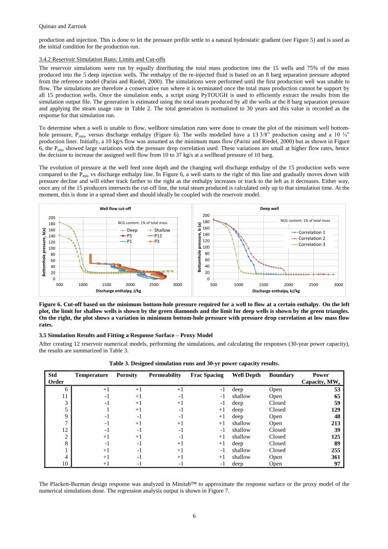
To determine when a well is unable to flow, wellbore simulation runs were done to create the plot of the minimum well bottom-

hole pressure, Pmin, versus discharge enthalpy (Figure 6). The wells modelled have a 13 3/8” production casing and a 10 ¾”

production liner. Initially, a 10 kg/s flow was assumed as the minimum mass flow (Parini and Riedel, 2000) but as shown in Figure

6, the Pmin showed large variations with the pressure drop correlation used. These variations are small at higher flow rates, hence

the decision to increase the assigned well flow from 10 to 37 kg/s at a wellhead pressure of 10 barg.

The evolution of pressure at the well feed zone depth and the changing well discharge enthalpy of the 15 production wells were

compared to the Pmin vs discharge enthalpy line. In Figure 6, a well starts to the right of this line and gradually moves down with

pressure decline and will either track farther to the right as the enthalpy increases or track to the left as it decreases. Either way,

once any of the 15 producers intersects the cut-off line, the total steam produced is calculated only up to that simulation time. At the

moment, this is done in a spread sheet and should ideally be coupled with the reservoir model.

Figure 6. Cut-off based on the minimum bottom-hole pressure required for a well to flow at a certain enthalpy. On the left

plot, the limit for shallow wells is shown by the green diamonds and the limit for deep wells is shown by the green triangles.

On the right, the plot shows a variation in minimum bottom-hole pressure with pressure drop correlation at low mass flow

rates.

3.5 Simulation Results and Fitting a Response Surface – Proxy Model

After creating 12 reservoir numerical models, performing the simulations, and calculating the responses (30-year power capacity),

the results are summarized in Table 3.

Table 3. Designed simulation runs and 30-yr power capacity results.

Std

Order

Temperature Porosity Permeability Frac Spacing Well Depth Boundary Power

Capacity, MWe

6 +1 +1 +1 -1 deep Open 53

11 -1 +1 -1 -1 shallow Open 65

3 -1 +1 +1 -1 deep Closed 59

5 1 +1 -1 +1 deep Closed 129

9 -1 -1 -1 +1 deep Open 48

7 -1 +1 +1 +1 shallow Open 213

12 -1 -1 -1 -1 shallow Closed 39

2 +1 +1 -1 +1 shallow Closed 125

8 -1 -1 +1 +1 deep Closed 89

1 +1 -1 +1 -1 shallow Closed 255

4 +1 -1 +1 +1 shallow Open 361

10 +1 -1 -1 -1 deep Open 97

The Plackett-Burman design response was analyzed in Minitab™ to approximate the response surface or the proxy model of the

numerical simulations done. The regression analysis output is shown in Figure 7.

500000 1000000 1500000 2000000 2500000 3000000

0

2000000

4000000

6000000

8000000

10000000

12000000

14000000

16000000

18000000

20000000

0

20

40

60

80

100

120

140

160

180

200

500 1000 1500 2000 2500 3000

Bo

tto

mh

ole

pre

ssu

re, b

(a)

Discharge enthalpy, J/kg

Well flow cut-off

Deep ShallowP5 P12P1 P3

NCG content: 1% of total mass

0

20

40

60

80

100

120

140

160

180

200

500 1000 1500 2000 2500 3000

Bo

tto

mh

ole

pre

ssu

re, b

(a)

Discharge enthalpy, kJ/kg

Deep well

Correlation 1Correlation 2Correlation 3

NCG content: 1% of total mass

Quinao and Zarrouk

7

Figure 7. Summary table of the polynomial fit between the response and the parameters.

The reservoir numerical simulations are approximated by a first-order proxy model using all the coded (-1, +1) parameters to

generate the response (Power Capacity). This is shown in Equation 4.

(4)

where A is reservoir temperature, B is matrix porosity, C is fracture permeability, D is average fracture spacing, E is well feed zone

depth, and F is boundary condition. This means a response may be estimated by replacing the variables with their coded value. The

polynomial coefficients were taken from the “Coef” column in Figure 7. Note that the ED chosen at the start of the analysis,

Plackett-Burman, limits the proxy model to a first-order polynomial because this design analyzes main effects only.

3.6 Analysis of the Main Effects and Response Surface

To screen out the main effects, the p-values (P) in the results table (see Figure 7) were checked to verify the parameters that are

statistically significant. The significance was set at a 95% confidence level so the p-values were compared to α-level of 0.05. All p-

values less than or equal to the α-level are significant while all p-values greater than the α-level are insignificant.

The regression model contained three significant parameters that affect the 30-yr power capacity estimate of the numerical

simulation: (1) well feed zone depth, (2) fracture permeability, and (3) reservoir temperature. The absolute values in the “Effects”

column show the relative strength of a parameter’s effect on the response. Well feed zone depth has the greatest effect (-97.28),

followed by fracture permeability (87.76), and reservoir temperature (84.49). From the sign of the effects, we can additionally infer

that using just deep production wells in the strategy results in lower power capacity, while finding high permeability (100 mD) and

high reservoir temperature (280°C) results in higher power capacity.

Figure 8. Pareto Chart and the Normal Plot of the effects showing the three significant parameters based on a 95%

confidence level (α = 0.05).

Fracture spacing does not meet the 95% interval but, as shown in Figure 7, has a p-value almost close to the required α level

of <0.05. Also, based on their p-values, porosity and boundary conditions are not significant. While α = 0.05 is typical of this type

of analysis, this shows that selecting a lower confidence level, for example α = 0.1, would have included fracture spacing as a

significant parameter and could be employed in such circumstances.

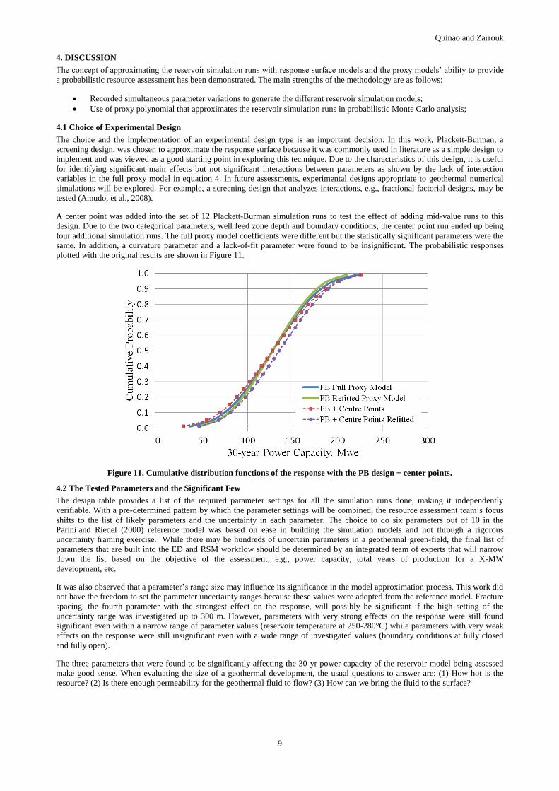
The validity of the regression and of the proxy model is verified by the plots of the residuals shown in Figure 9. The plots show that

the errors are normally distributed and are independent of each other. It should be noted here that numerical simulation experiments

do not have a random error or measurement error (Sacks, et. al., 1989; Myers and Montgomery, 2002) and the error is mainly from

fitting the wrong proxy polynomial or the choice of parameters to include in polynomial fitting.

Quinao and Zarrouk

8

Figure 9. Residual plots showing residuals on a normal plot, residuals and fits, histogram of the residuals, and residuals

versus the order simulations were performed.

3.7 Refitting the Response Surface with Only the Significant Parameters

Keeping the full response equation might be a good idea for the particular purpose of approximating the reservoir simulation

response to the tested parameters (Myers and Montgomery, 2002). Refitting the proxy model to the significant parameters

simplifies the model to the main effects terms. Also, if a more detailed design like CCD or Box-Behnken is required in the analysis,

the workflow suggests applying the design to the significant parameters. A similar issue about keeping the full model or refitting

was discussed by Anderson and Whitcomb (2005). To compare, we refitted the model using only the significant terms, the

response polynomial of coded parameters becomes:

(5)

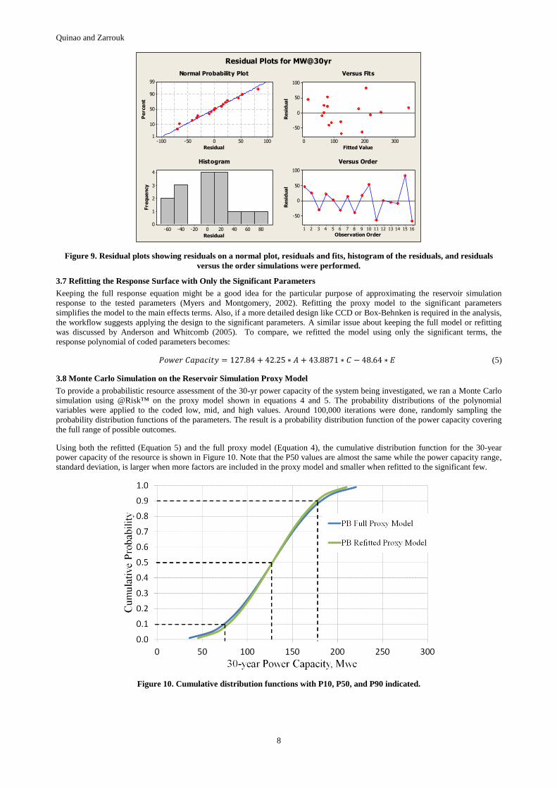
3.8 Monte Carlo Simulation on the Reservoir Simulation Proxy Model

To provide a probabilistic resource assessment of the 30-yr power capacity of the system being investigated, we ran a Monte Carlo

simulation using @Risk™ on the proxy model shown in equations 4 and 5. The probability distributions of the polynomial

variables were applied to the coded low, mid, and high values. Around 100,000 iterations were done, randomly sampling the

probability distribution functions of the parameters. The result is a probability distribution function of the power capacity covering

the full range of possible outcomes.

Using both the refitted (Equation 5) and the full proxy model (Equation 4), the cumulative distribution function for the 30-year

power capacity of the resource is shown in Figure 10. Note that the P50 values are almost the same while the power capacity range,

standard deviation, is larger when more factors are included in the proxy model and smaller when refitted to the significant few.

Figure 10. Cumulative distribution functions with P10, P50, and P90 indicated.

100500-50-100

99

90

50

10

1

ResidualP

erce

nt

3002001000

100

50

0

-50

Fitted Value

Re

sid

ua

l

806040200-20-40-60

4

3

2

1

0

Residual

Fre

qu

en

cy

16151413121110987654321

100

50

0

-50

Observation Order

Re

sid

ua

l

Normal Probability Plot Versus Fits

Histogram Versus Order

Residual Plots for MW@30yr

Quinao and Zarrouk

9

4. DISCUSSION

The concept of approximating the reservoir simulation runs with response surface models and the proxy models’ ability to provide

a probabilistic resource assessment has been demonstrated. The main strengths of the methodology are as follows:

Recorded simultaneous parameter variations to generate the different reservoir simulation models;

Use of proxy polynomial that approximates the reservoir simulation runs in probabilistic Monte Carlo analysis;

4.1 Choice of Experimental Design

The choice and the implementation of an experimental design type is an important decision. In this work, Plackett-Burman, a

screening design, was chosen to approximate the response surface because it was commonly used in literature as a simple design to

implement and was viewed as a good starting point in exploring this technique. Due to the characteristics of this design, it is useful

for identifying significant main effects but not significant interactions between parameters as shown by the lack of interaction

variables in the full proxy model in equation 4. In future assessments, experimental designs appropriate to geothermal numerical

simulations will be explored. For example, a screening design that analyzes interactions, e.g., fractional factorial designs, may be

tested (Amudo, et al., 2008).

A center point was added into the set of 12 Plackett-Burman simulation runs to test the effect of adding mid-value runs to this

design. Due to the two categorical parameters, well feed zone depth and boundary conditions, the center point run ended up being

four additional simulation runs. The full proxy model coefficients were different but the statistically significant parameters were the

same. In addition, a curvature parameter and a lack-of-fit parameter were found to be insignificant. The probabilistic responses

plotted with the original results are shown in Figure 11.

Figure 11. Cumulative distribution functions of the response with the PB design + center points.

4.2 The Tested Parameters and the Significant Few

The design table provides a list of the required parameter settings for all the simulation runs done, making it independently

verifiable. With a pre-determined pattern by which the parameter settings will be combined, the resource assessment team’s focus

shifts to the list of likely parameters and the uncertainty in each parameter. The choice to do six parameters out of 10 in the

Parini and Riedel (2000) reference model was based on ease in building the simulation models and not through a rigorous

uncertainty framing exercise. While there may be hundreds of uncertain parameters in a geothermal green-field, the final list of

parameters that are built into the ED and RSM workflow should be determined by an integrated team of experts that will narrow

down the list based on the objective of the assessment, e.g., power capacity, total years of production for a X-MW

development, etc.

It was also observed that a parameter’s range size may influence its significance in the model approximation process. This work did

not have the freedom to set the parameter uncertainty ranges because these values were adopted from the reference model. Fracture

spacing, the fourth parameter with the strongest effect on the response, will possibly be significant if the high setting of the

uncertainty range was investigated up to 300 m. However, parameters with very strong effects on the response were still found

significant even within a narrow range of parameter values (reservoir temperature at 250-280°C) while parameters with very weak

effects on the response were still insignificant even with a wide range of investigated values (boundary conditions at fully closed

and fully open).

The three parameters that were found to be significantly affecting the 30-yr power capacity of the reservoir model being assessed

make good sense. When evaluating the size of a geothermal development, the usual questions to answer are: (1) How hot is the

resource? (2) Is there enough permeability for the geothermal fluid to flow? (3) How can we bring the fluid to the surface?

Quinao and Zarrouk

10

4.3 The Proxy Models and the Volumetric Stored-heat/Mass in Place

The probabilistic resource assessment based on ED and RSM proxy models were compared with the probabilistic resource

assessments based on volumetric stored heat and combined volumetric/numerical simulation methods. The parameters that were

varied were limited to the parameters chosen in the ED and RSM workflow, i.e., reservoir area and thickness were kept constant.

Table 4. Parameters used in the volumetric stored heat and the volumetric/numerical simulation probabilistic analyses.

Parameters Low Mid High Distribution

Co

mm

on

to

bo

th Area, km2 -- 9 -- N.A.

Thickness, km -- 1.14 -- N.A.

Average porosity 0.05 0.08 0.1 Triangular

Reservoir Temperature, °C 250 265 280 Triangular

Reject Temperature, °C -- 175.36 -- N.A.

Rock heat capacity, J/kg -- 1000 -- N.A.

Rock density, kg/m3 -- 2600 -- N.A.

Plant load factor -- 0.85 -- N.A.

Project life, years -- 30 -- N.A.

Stored

heat

Recovery factor, stored-heat1 0.1 0.15 0.5 Triangular

Conv. efficiency (stored heat)2 -- 0.12 -- N.A.

Vol/

numerical

Recovery factor,

(volumetric/numerical)3 0.205 0.468 0.75 Triangular

Steam usage rate, kg steam/kW -- 7.5 -- N.A. 1The stored heat recovery factor parameter range was based on the review done by Zarrouk and Simiyu (2013). 2Conversion

efficiency is based on review by Zarrouk and Moon (2013). 3Mass in place recovery factor was parameterized by Parini and

Riedel (2000) but no proxy polynomial was published so this range was estimated from the main effects plot between parameters

and % recovery.

The results of the different probabilistic resource assessments are shown in Figure 12.

Figure 12. ED and RSM, stored heat, and volumetric/numerical cumulative distribution functions.

The comparison showed in Figure 12 should be limited to a simple illustration of the different probabilistic assessment results and

how similar methods—(1) volumetric stored heat with volumetric/numerical simulation and (2) ED/RSM proxy model and

volumetric/numerical simulation—result in different estimates due to different assumptions in the methodologies. The volumetric

stored heat had the lowest power capacity range due to the lower range of thermal recovery factors and is probably due to the lower

conversion efficiency used. The other two methods have recharge components providing them access to a larger fluid volume.

Although the ED and RSM proxy model was based on the volumetric and numerical simulation model, the implementations of the

numerical simulations were different. The simplification done by estimating the mass in place recovery factors from the published

main effects plots (Parini and Riedel, 2000) and assigning a triangular probability distribution to the parameter was a large

assumption.

Quinao and Zarrouk

11

5. CONCLUSION

A probabilistic resource assessment methodology based on numerical simulations was demonstrated using an experimental design

and response surface method (ED and RSM) workflow. The strength of the workflow lies in the experimental design’s ability to be

independently verified because the parameter settings and combinations are recorded in the design table. The response surface or

proxy model is a good approximation of the relationship between the response and the tested parameters generated from reservoir

numerical simulations. There are existing commercial software packages that can be used to implement the ED workflow in

geothermal reservoir simulation though the process is still manual and inefficient. In this scenario, resource assessment specialists

can focus more on refining the list of parameters and the range and distribution of parameter uncertainties because the design

pattern is available.

6. NEXT PHASE

In the next stage of the study the ED and RSM workflow will be improved and tested on a large numerical model of a geothermal

green-field and will transition out of the commercial software packages into available open-source codes. Appropriate experimental

designs will be explored. A response surface method (RSM) experimental design, with quadratic proxy models, will be tested to

evaluate the possible optimization of controllable parameters e.g. the impact of well depths and the impact of well spacing. Also, a

more efficient way of implementing the workflow, e.g., building the numerical simulation runs through PyTOUGH

(O’Sullivan et al., 2013), will be explored.

7. ACKNOWLEDGMENT

The authors would like to thank Mighty River Power Ltd. for supporting the work and allowing us full use of software licenses

during this part of the study. The authors would also like to thank Lutfhie Sirad-Azwar for valuable discussions on process

modeling and Peter Franz for invaluable assistance with PyTOUGH.

REFERENCES

Acuña, J., Parini, M., and Urmeneta, N.: Using a Large Reservoir Model in the Probabilistic Assessment of Field Management

Studies, Proceedings, 27th Workshop on Geothermal Reservoir Engineering, Stanford University, Stanford, CA (2002).

Amudo, C., Graf, T., Dandekar, R., and Randle, J.M.: The Pains and Gains of Experimental Design and Response Surface

Applications in Reservoir Simulation Studies, paper SPE 118709, presented at the 2009 SPE Reservoir Simulation

Symposium, The Woodlands, Texas, February 2-4.

Anderson, M., and Whitcomb, P.: DOE Simplified: Practical Tools for Effective Experimentation, Productivity, Inc., Portland

(2000).

Anderson, M., and Whitcomb, P.: RSM Simplified: Optimizing Processes Using Response Surface Methods for Design of

Experiments, Productivity, Inc., New York (2005).

Atkinson, P.: Proved Geothermal Reserves – Framework and Methodology, Proceedings, New Zealand Geothermal Workshop,

Auckland (2012).

Australian Geothermal Reporting Code Committee (AGRCC): Geothermal Lexicon for Resources and Reserves Definition and

Reporting, 2nd ed., Adelaide (2010).

Clearwater, J., Burnell, J., and Sirad-Azwar, L.: Modelling the Ngatamariki Geothermal System, Proceedings, New Zealand

Geothermal Workshop, Auckland (2011).

Croucher, A.: PyTOUGH: A Python Scripting Library for Automating TOUGH2 Simulations, Proceedings, New Zealand

Geothermal Workshop, Auckland (2011).

Damsleth, E., Hage, A., and Volden, R.: Maximum Information at Minimum Cost: A North Sea Field Development Study With an

Experimental Design, JPT, (December 1992), 1350-1356.

Friedmann, F., Chawathé, A., and Larue, D.K.: Assessing Uncertainty in Channelized Reservoirs Using Experimental Designs, SPE

Reservoir Evaluation and Engineering (August 2003), 264-274.

Garg, S.: Appropriate Use of the USGS Volumetric “Heat In Place” Method and Monte Carlo Calculations, Proceedings, 35th

Workshop on Geothermal Reservoir Engineering, Stanford University, Stanford, CA (2010).

Garg, S., and Combs, J.: A Reexamination of USGS Volumetric “Heat In Place” Method, Proceedings, 36th Workshop on

Geothermal Reservoir Engineering, Stanford University, Stanford, CA (2011).

Grant, M., and Mahon, T.: A Probabilistic Approach to Field Proving and Station Sizing, Geothermal Resources Council

Transactions, 19, (1995).

Grant, M.: Geothermal Resource Proving Criteria, Proceedings, World Geothermal Congress, Kyushu-Tohoku (2000).

Hoang, V., Alamsyah, O., and Roberts, J.: Darajat Geothermal Field Performance-A Probabilistic Forecast, Proceedings, World

Geothermal Congress, Antalya (2005).

Myers, R., and Montgomery, D.: Response Surface Methodology-Process and Product Optimization Using Designed Experiments,

2nd ed., John Wiley & Sons, Inc., New York City (2002).

Onur, M., Sarak, H., and Türeyen, İ.: Probabilistic Resource Estimation of Stored and Recoverable Thermal Energy for Geothermal

Systems by Volumetric Methods, Proceedings, World Geothermal Congress, Bali (2010).

Quinao and Zarrouk

12

O'Sullivan, J., Dempsey, D., Croucher, A.E., Yeh, A. and O'Sullivan, M.J.: Controlling Complex Geothermal Simulations Using

PyTOUGH, Proceedings, 38th Workshop on Geothermal Reservoir Engineering, Stanford University, Stanford, CA (2013).

Parini, M., Pisani, P., Monterrosa, M.: Resource Assessment at the Berlin Geothermal Field (El Salvador), Proceedings, World

Geothermal Congress, Firenze (1995).

Parini, M., and Riedel, K.: Combining Probabilistic Volumetric and Numerical Simulation Approaches to Improve Estimates of

Geothermal Resource Capacity, Proceedings, World Geothermal Congress, Kyushu-Tohoku (2000).

Pruess, K., Oldenburg, C., and Moridis, G.: TOUGH2 User’s Guide, Version 2.0, Report LBNL-43134, Lawrence Berkeley

National Laboratory, University of California, Berkeley, CA (1999).

R Core Team: R: A Language and Environment for Statistical Computing. R Foundation for Statistical Computing, Vienna, ISBN

3-900051-07-0, http://www.R-project.org/ (2013).

Sacks, J., Schiller, S., and Welch, W.: Design for Computer Experiments, Technometrics, 31, (February 1989) 41-47.

Sanyal, S., and Sarmiento, Z.: Booking Geothermal Energy Reserves. GRC Transactions, 29, (2005) 467-474.

Walpole, R., Myers, R., Myers, S., Ye, K.: Probability & Statistics for Engineers and Scientists, 9th ed., Prentice Hall, Boston

(2012).

White, C., and Royer, S.: Experimental Design as Framework for Reservoir Studies, paper SPE 79676, presented at the 2003 SPE

Reservoir Simulation Symposium, Houston, February 2-5.

Williams, C.., Reed, M., and Mariner, R.: A Review of the Methods Applied by the U.S. Geological Survey in the Assessment of

Identified Geothermal Resources, U.S. Geological Survey Open-File Report 2008-1296, 27p. (2008).

Yeten, B., Castellini, A., Guyaguler, B., and Chen, W.H.: A Comparison on Experimental Design and Response Surface

Methodologies, paper SPE 93347, presented at the 2005 SPE Reservoir Simulation Symposium, Houston, January 31 –

February 2.

Zarrouk, S., and Moon, H.: Efficiency of Geothermal Power Plants: A worldwide review, Geothermics, 51, (2013) 142-153.

Zarrouk, S., and Simiyu, F.: A Review of Geothermal Resource Estimation Methodology, Proceedings, New Zealand Geothermal

Workshop, Rotorua (2013).