Application-Specific Configuration

Selection in the Cloud: Impact of

Provider Policy and Potential of

Systematic Testing

Mohammad Hajjat+, Ruiqi Liu*, Yiyang Chang+, T.S. Eugene Ng*, Sanjay Rao+

+ Purdue University, * Rice University

Overview

2

Cloud users face many choices when deploying applications in the cloud • VM size • CPU heterogeneity

Cloud providers employ complex policies • Bandwidth rate limit • VM packing • CPU scheduling

Goal • Understand how policies can impact performance • Select good configurations for applications

Related work

• “Trial and error” strategies replace bad VMs with good VMs

• Heavy weight testing strategy profiles cost-performance of different VM sizes and migrates applications

• Our systematic testing techniques – Consider both VM size and CPU type – Advantageous for stateful applications that are

hard to migrate

38

Contributions

• Conducted large scale 19-month measurement study of Amazon EC2

• Found that provider policy impacts configuration choices in surprising ways – Larger VM sizes do not necessarily see higher bandwidth

• Proposed and evaluated configuration selection techniques systematically – Iprune reduces the number of tests by 40% - 70% – Nearest Neighbor selects the configuration within 6% of best

for 80% cases with no testing overhead

3

Amazon EC2 VMs

• General purpose EC2 VMs (M1) have four sizes: small (S), medium (M), large (L), extra-large (X)

• VMs of the same size may be hosted with different types of CPUs

5

Abbreviation CPU (Intel Xeon) Speed (GHz) Release Cores

A E5430 2.66 Q4 2007 4 B E5645 2.40 Q1 2010 6 C E5507 2.26 Q1 2010 4 D E5-2650 2.00 Q1 2012 8

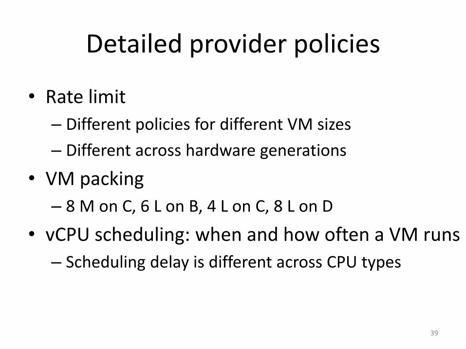
Detailed provider policies

• Rate limit – Different policies for different VM sizes – Different across hardware generations

• VM packing – 8 M on C, 6 L on B, 4 L on C, 8 L on D

• vCPU scheduling: when and how often a VM runs – Scheduling delay is different across CPU types

39

Impact of VM packing

40

8 MC VMs on a physical machine

4 LC VMs on a physical machine

Impact of VM packing

41

8 MC VMs on a physical machine

4 LC VMs on a physical machine

2 Gbps shared by 8 VMs 2 Gbps shared by 4 VMs

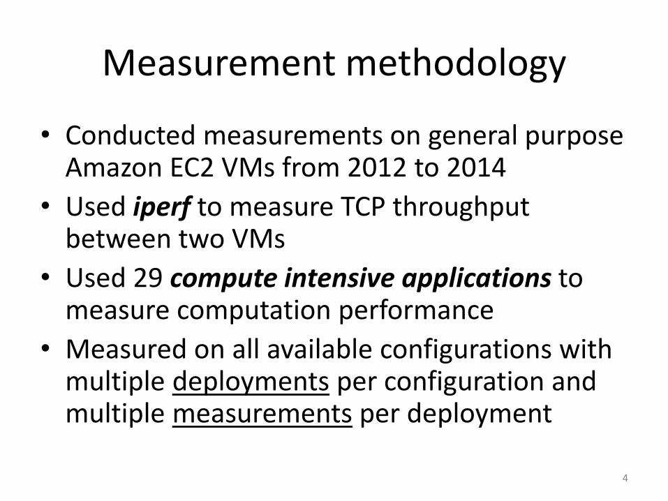
Measurement methodology

• Conducted measurements on general purpose Amazon EC2 VMs from 2012 to 2014

• Used iperf to measure TCP throughput between two VMs

• Used 29 compute intensive applications to measure computation performance

• Measured on all available configurations with multiple deployments per configuration and multiple measurements per deployment

4

Configuration Notations

• A configuration is the combination of VM size and CPU type – MC is a medium VM with CPU type C – For bandwidth measurement, two VMs are used.

Small AC means source is SA and destination is SC.

6

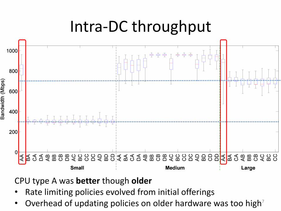
Intra-DC throughput

CPU type A was better though older

• Rate limiting policies evolved from initial offerings • Overhead of updating policies on older hardware was too high 7

Intra-DC throughput

M achieved higher bandwidth than L

8

Rate limit for L

Rate limit for S

Rate limit behavior on M and L • Conducted extensive study with dedicated

VMs which isolate multi-tenancy

9

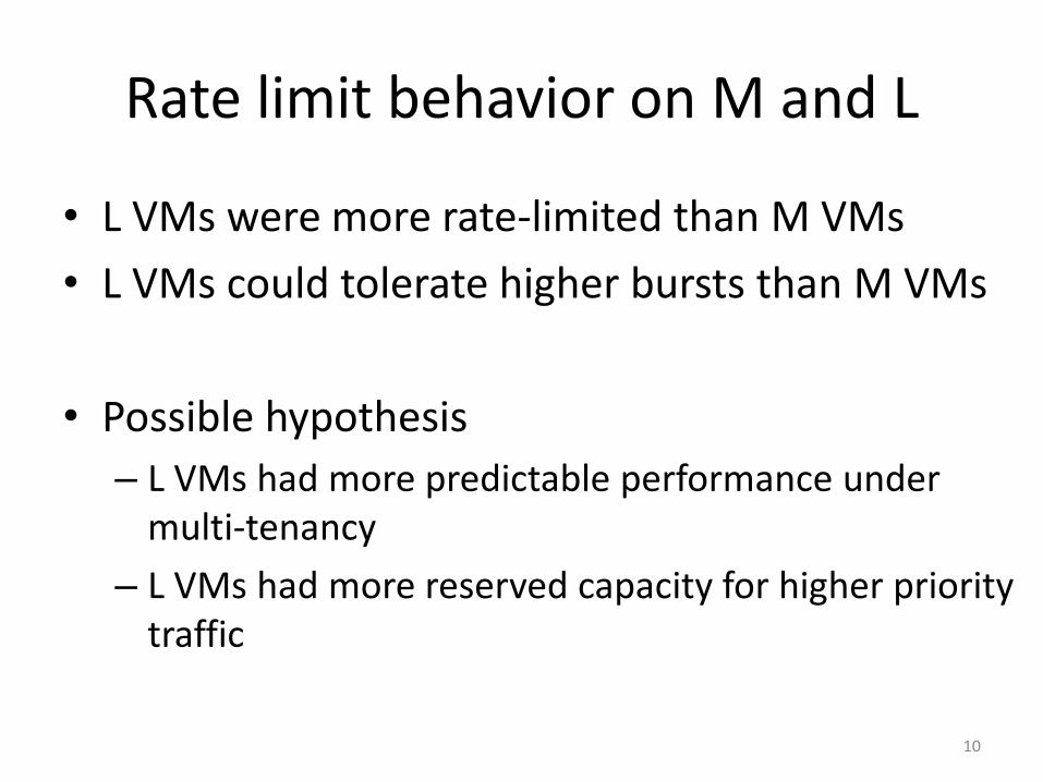
Rate limit behavior on M and L

• L VMs were more rate-limited than M VMs • L VMs could tolerate higher bursts than M VMs

• Possible hypothesis – L VMs had more predictable performance under

multi-tenancy – L VMs had more reserved capacity for higher priority

traffic

10

Inter-DC throughput

42

- CPU type on the receiver side matters

Compute intensive applications: MC was better than LC

11

MC is better than LC

• Conducted auxiliary measurement on MC and LC – Measured the time to run constant multiplication – Measured memory access latency for all memory

hierarchies using lmbench

• Findings – MC took less time than LC for multiplication – MC had lower access latency and less variation

12

Other findings • Inter-DC throughput closely related to the CPU type of the

receivers – Verified with UDP loss rate and traceroute data

• VM packing policies affected per-VM bandwidth – Verified with dedicated VMs locating on one physical machine

• CPU types A and C were more likely to experience high scheduling delay – Measured the actual elapsed time when having a process

sleep for a short period • Two cores on LC were scheduled in a more relaxed way

than on LA, LB and LD – Measured the delay when two threads started running

13

Configuration selection is non-trivial, and systematic testing is necessary

Interplay of VM size, CPU type and provider

policy impacts communication and computation performance

14

Systematic testing

• Goal: select the configuration (combination of CPU type and VM size) that takes least time and/or money for an application

15

Systematic testing

• Goal: select the configuration (combination of CPU type and VM size) that takes least time and/or money for an application

• Straw man – Per-Configuration testing (PerConfig)

• More intelligent systematic testing techniques – Iterative pruning (iPrune) – Nearest Neighbor shortlisting

16

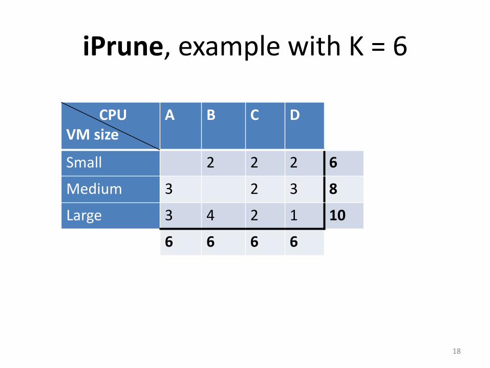
iPrune, example with K = 6

• Requirement: at least K deployments per choice in each configuration dimension

• Conduct M measurements per deployment • Deployments # = K ×max{|d1|, |d2|, . . . , |dn|}

17

CPU

VM size

A B C D

Small 2 2 2 6

Medium 3 2 3 8

Large 3 4 2 1 10

6 6 6 6

CPU

VM size

A B C D

Small 2 2 2 6

Medium 3 2 3 8

Large 3 4 2 1 10

6 6 6 6

iPrune, example with K = 6

18

CPU

VM size

A B C D

Small 2 2 2 6

Medium 3 2 3 8

Large 3 4 2 1 10

6 6 6 6

iPrune, example with K = 6

• Mark poor choices in each dimension for pruning – A is worse than B with a probability higher than 0.9,

so A is pruned

19

iPrune, example with K = 6

20

CPU

VM size

A B C D

Small 2 2 2 6

Medium 3 2 3 8

Large 3 4 2 1 10

6 6 6 6

• Mark poor choices in each dimension for pruning – Large is worse than medium with a probability higher

than 0.9, so large is pruned

iPrune, example with K = 6

21

CPU

VM size

A B C D

Small 2 2 2 6

Medium 3 2 3 5

Large 3 4 2 1 7

6 2 4 5

• Mark poor choices in each dimension for pruning – Large is worse than medium with a probability higher

than 0.9, so large is pruned

iPrune, example with K = 6

• Get more deployments to satisfy K

22

CPU

VM size

A B C D

Small 2 2 2 6

Medium 3 2 3 5

Large 3 4 2 1 10

6 2 4 5

CPU

VM size

A B C D

Small 5 2 2 9

Medium 3 1 4 4 9

Large 3 4 2 1 7

6 6 6 6

CPU

VM size

A B C D

Small 5 2 2 9

Medium 3 1 4 4 9

Large 3 4 2 1 10

6 6 6 6

CPU

VM size

A B C D

Small 5 2 2 7

Medium 3 1 4 4 5

Large 3 4 2 1 10

6 6 6 6

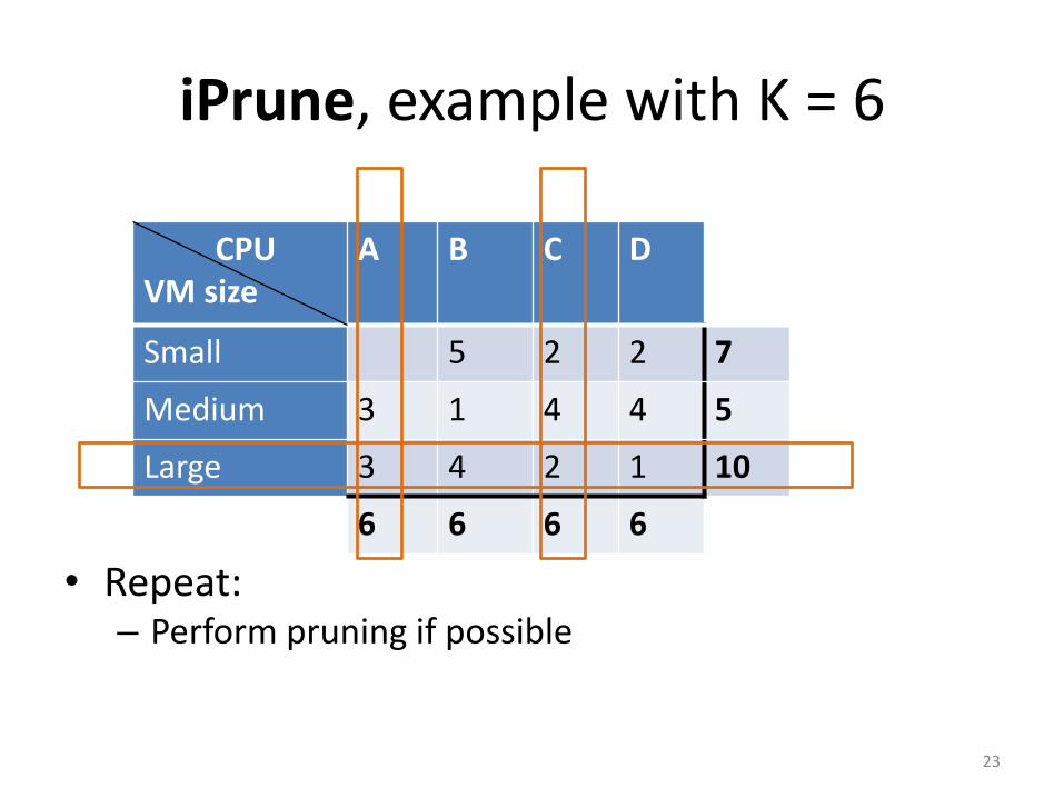
iPrune, example with K = 6

• Repeat: – Perform pruning if possible – Get more deployments if needed

23

CPU

VM size

A B C D

Small 5 2 2 9

Medium 3 1 4 4 9

Large 3 4 2 1 10

6 6 6 6

CPU

VM size

A B C D

Small 5 2 2 7

Medium 3 1 4 4 5

Large 3 4 2 1 10

6 6 6 6

CPU

VM size

A B C D

Small 5 2 2 7

Medium 3 2 4 4 6

Large 3 4 2 1 10

6 7 6 6

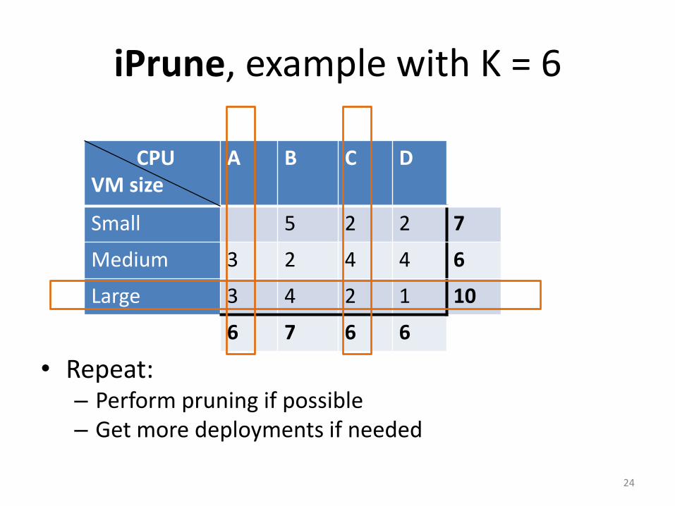
iPrune, example with K = 6

• Repeat: – Perform pruning if possible – Get more deployments if needed

24

iPrune, example with K = 6

• Finally: choose best configuration in each dimension

25

CPU

VM size

A B C D

Small 5 2 2 7

Medium 3 2 4 4 6

Large 3 4 2 1 10

6 7 6

iPrune vs PerConfig

PerConfig iPrune

iPerf 3000+ 700 Cassandra 1800 1000

26

• Evaluated with iperf and Cassandra – iperf measures TCP throughput for a pair of VMs – Cassandra is a key-value store, measured with

YCSB workloads (read + write)

Number of tests for 5% error target

Systematic testing techniques

27

iPrune ͻConservatively prunes out bad VMs

Nearest Neighbor ͻProactively shortlists good VMs ͻUses performance data of existing apps ͻAssumption ͻSimilar applications tend to have

similar best configurations

Nearest Neighbor Attribute3

Attribute1 Attribute2

T

28

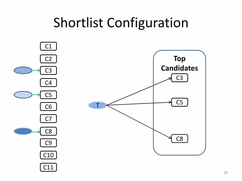
Shortlist Configuration

29

T

C3

C5

C8

Top

Candidates

C1

C2

C3

C4

C5

C6

C7

C8

C9

C10

C11

Shortlist Configuration

30

T

Time=560s

Time=700s

Time=450s

C3

C5

C8

Top

Candidates

C1

C2

C3

C4

C5

C6

C7

C8

C9

C10

C11

Shortlist Configuration

31

T

Time=560s

Time=700s

Time=450s

C3

C5

C8

Top

Candidates

Low / no

overhead

High

accuracy

C1

C2

C3

C4

C5

C6

C7

C8

C9

C10

C11

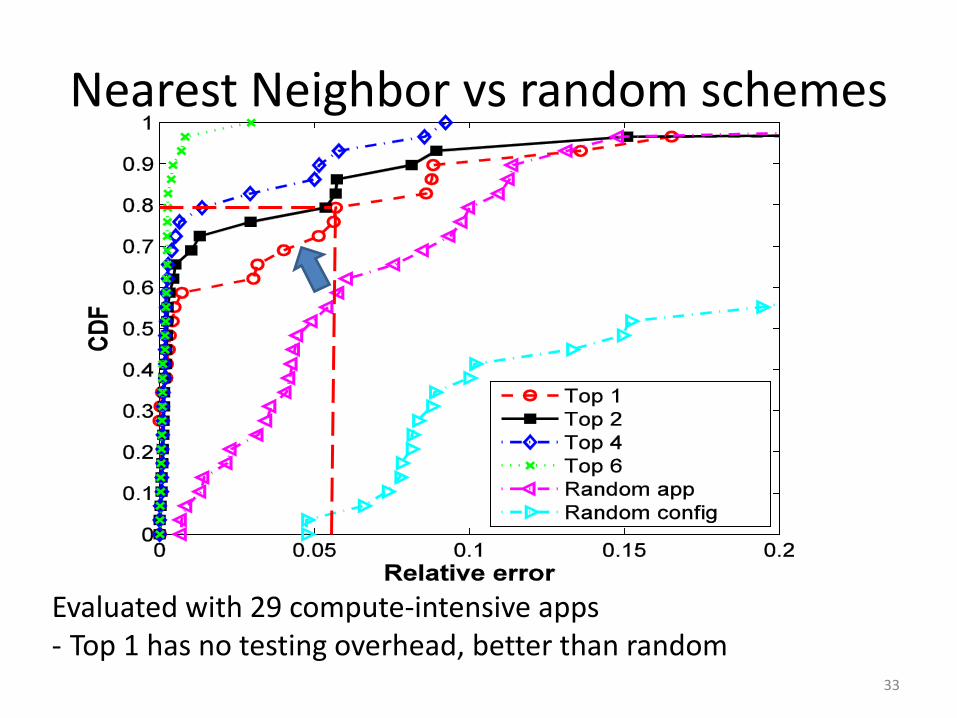
Nearest Neighbor vs random schemes

32

Evaluated with 29 compute-intensive apps

Nearest Neighbor vs random schemes

33

Evaluated with 29 compute-intensive apps - Top 1 has no testing overhead, better than random

Nearest Neighbor vs random schemes

34

Evaluated with 29 compute-intensive apps - Top 1 has no testing overhead, better than random - More top candidates, greater testing overhead, higher accuracy

Implications of Nearest Neighbor

• Make a tradeoff between testing overhead and accuracy of the selected configuration

• Top 1 is promising for short running applications – No testing overhead, good configuration

• More top candidates is better for long running applications – Higher tolerance for testing overhead, higher

accuracy of the selected configuration

35

Conclusions

• Provider policy affects the performance of applications in unexpected ways – Analyzed through large scale measurement study

of Amazon EC2 • iPrune greatly reduces testing overhead – Iprune reduces the number of tests by 40% - 70%

• Nearest Neighbor incurs low testing overhead and achieves high accuracy – Nearest Neighbor selects the configuration within

6% of best for 80% cases with no testing overhead

36