Application of Wind Fetch and Wave Models for Habitat - USGS
54
In cooperation with the U.S. Army Corps of Engineers Application of Wind Fetch and Wave Models for Habitat Rehabilitation and Enhancement Projects U.S. Department of the Interior U.S. Geological Survey Open-File Report 2008–1200 659 658 657 656 Weighted Wind Fetch LOW HIGH
Transcript of Application of Wind Fetch and Wave Models for Habitat - USGS

In cooperation with the U.S. Army Corps of Engineers
Application of Wind Fetch and Wave Models for Habitat Rehabilitation and Enhancement Projects
U.S. Department of the InteriorU.S. Geological Survey
Open-File Report 2008–1200
659
658
657
656
Weighted Wind FetchLOW HIGH

Cover. Depiction of management scenario 4, weighted wind fetch results for the Capoli Slough Habitat Rehabilitation and Enhancement Project in Navigation Pool 9, Upper Mississippi River System. The background image is a grayscale version of a 2006 National Agriculture Imagery Program aerial photograph.

Application of Wind Fetch and Wave Models for Habitat Rehabilitation and Enhancement Projects
By Jason Rohweder, James T. Rogala, Barry L. Johnson, Dennis Anderson,
Steve Clark, Ferris Chamberlin, and Kip Runyon
In cooperation with the U.S. Army Corps of Engineers
Open-File Report 2008–1200
U.S. Department of the InteriorU.S. Geological Survey

U.S. Department of the InteriorDIRK KEMPTHORNE, Secretary
U.S. Geological SurveyMark D. Myers, Director
U.S. Geological Survey, Reston, Virginia: 2008
For product and ordering information: World Wide Web: http://www.usgs.gov/pubprod Telephone: 1-888-ASK-USGS
For more information on the USGS—the Federal source for science about the Earth, its natural and living resources, natural hazards, and the environment: World Wide Web: http://www.usgs.gov Telephone: 1-888-ASK-USGS
Any use of trade, product, or firm names is for descriptive purposes only and does not imply endorsement by the U.S. Government.
Although this report is in the public domain, permission must be secured from the individual copyright owners to reproduce any copyrighted materials contained within this report.
Suggested citation: Rohweder, Jason, Rogala, James T., Johnson, Barry L., Anderson, Dennis, Clark, Steve, Chamberlin, Ferris, and Runyon, Kip, 2008, Application of wind fetch and wave models for habitat rehabilitation and enhancement projects: U.S. Geological Survey Open-File Report 2008–1200, 43 p.

iii
Contents
Abstract ...........................................................................................................................................................1Introduction.....................................................................................................................................................1Toolbox Installation ........................................................................................................................................1Wind Fetch Model..........................................................................................................................................3
Introduction............................................................................................................................................3Methodology ..........................................................................................................................................3Wind Fetch Model Validation ..............................................................................................................5
Two-Sample Permutation Test for Locations ..........................................................................8Wave Model ....................................................................................................................................................8
Introduction............................................................................................................................................8Assumptions and Model Limitations ...............................................................................................11Methodology ........................................................................................................................................11
Adjusting Wind Speed Data .....................................................................................................11Deep Water Test ........................................................................................................................12Significant Wave Height ...........................................................................................................14Wave Length ...............................................................................................................................15Spectral Peak Wave Period .....................................................................................................15Maximum Orbital Wave Velocity .............................................................................................15Shear Stress ...............................................................................................................................15
St. Paul District Analyses ...........................................................................................................................17Study Areas..........................................................................................................................................17
Capoli Slough Habitat Rehabilitation and Enhancement Project ......................................17Harpers Slough Habitat Rehabilitation and Enhancement Project ...................................19
Weighted Wind Fetch Analysis ........................................................................................................21Land Raster Input Data .............................................................................................................21Wind Direction Input Data ........................................................................................................21Weighted Wind Fetch ................................................................................................................23Analysis Results .........................................................................................................................24Discussion ...................................................................................................................................24
Sediment Suspension Probability Analysis ....................................................................................24Analysis Results .........................................................................................................................29Discussion ...................................................................................................................................34
St. Louis District Analysis ...........................................................................................................................34Study Area............................................................................................................................................34
Swan Lake Habitat Rehabilitation and Enhancement Project ...........................................34Weighted Wind Fetch Analysis ........................................................................................................35
Land Raster Input Data .............................................................................................................35U.S. Fish and Wildlife Service Sample Island Design ..........................................................36U.S. Army Corps of Engineers Sample Island Design ..........................................................36Wind Direction Input Data ........................................................................................................37Weighted Wind Fetch ................................................................................................................37Analysis Results .........................................................................................................................40Discussion ...................................................................................................................................40

iv
Spatial Datasets Used in Analyses ...........................................................................................................40Long Term Resource Monitoring Program 2000 Land Cover/Land Use Data
for the Upper Mississippi River System ............................................................................40Originator.....................................................................................................................................40Abstract .......................................................................................................................................40Online Linkage ............................................................................................................................40
Long Term Resource Monitoring Program Bathymetric Data for the Upper Mississippi and Illinois Rivers .................................................................................40
Originator.....................................................................................................................................40Abstract .......................................................................................................................................40Online Linkage ............................................................................................................................40
Acknowledgments .......................................................................................................................................43References Cited..........................................................................................................................................43
Figures 1–5. Screen shots showing: 1. Windows Explorer view of extracted files.......................................................................2 2. ArcToolbox view of wave tools .........................................................................................2 3. Windows dialog box for selecting Waves toolbox .........................................................3 4. Sample text file with fetch direction input data .............................................................3 5. Fetch model dialog window prompting user input .........................................................4 6. Diagram showing example depictions of wind fetch calculated using the
different methods ..........................................................................................................................5 7. Map showing sample wind fetch model results for Swan Lake Habitat
Rehabilitation and Enhancement Project (HREP) ....................................................................6 8. Map showing wind fetch cell locations and prevailing wind directions used for
model validation ............................................................................................................................7 9. Graph showing results for two-sample permutation test for locations ..............................9 10. Screen shot showing wave model dialog window prompting user input .........................10 11. Screen shot showing sample text file depicting valid input values for wind data
in wave model .............................................................................................................................10 12. Map showing visual depiction of Navigation and Ecosystem Sustainability
Program subareas used to calculate average water depth ................................................13 13. Map showing sample wave model outputs for scenario 4, Capoli Slough
HREP .............................................................................................................................................16 14. Diagram depicting relationships of input and output parameters used within
the wave model ...........................................................................................................................17 15–17. Maps showing: 15. Location of Pool 9 Capoli Slough and Harpers Slough HREPs ...................................18 16. Capoli Slough HREP with feature labels ........................................................................19 17. Harpers Slough HREP with feature labels .....................................................................20 18. Aerial photograph showing location of revised island addition to Harpers Slough
HREP area ....................................................................................................................................21 19. Sample copy of a National Climatic Data Center, Local Climatological Data
summary sheet ............................................................................................................................22 20. Graph showing breakdown of wind directions collected for La Crosse
Municipal Airport site ................................................................................................................23

v
21. Screen shot showing weighted sum dialog window example ...........................................23 22–24. Maps showing: 22. Weighted wind fetch results for the Capoli Slough HREP ..........................................25 23. Weighted wind fetch results for the Harpers Slough HREP .......................................26 24. Difference in weighted wind fetch from the existing conditions
management scenario to scenarios 1, 2, 3, and 4 for the Capoli Slough HREP ...........................................................................................................27
25. Graph showing numerical difference in weighted wind fetch from the existing conditions management scenario to scenarios 1, 2, 3, and 4 for the Capoli Slough HREP ....................................................................................................................27
26. Map showing difference in weighted wind fetch from the existing conditions management scenario to scenarios 1, 2, 3, and 4 for the Harpers Slough HREP ............28
27. Graph showing numerical difference in weighted wind fetch from the existing conditions management scenario to scenarios 1, 2, 3, and 4 for the Harpers Slough HREP ................................................................................................................28
28. Diagram explaining process for calculating percent of days capable of suspending sediments ...............................................................................................................29
29–31. Maps showing: 29. Sediment suspension probability results for the Capoli Slough HREP .....................30 30. Sediment suspension probability results for the Harpers Slough HREP ..................31 31. Difference in sediment suspension probability from the existing
conditions management scenario to scenarios 1, 2, 3, and 4 for the Capoli Slough HREP ...........................................................................................................32
32. Graph showing numerical difference in sediment suspension probability from the existing conditions management scenario to scenarios 1, 2, 3, and 4 for the Capoli Slough HREP .......................................................................................................32
33. Map showing difference in sediment suspension probability from the existing conditions management scenario to scenarios 1, 2, 3, and 4 for the Harpers Slough HREP ................................................................................................................33
34. Graph showing numerical difference in sediment suspension probability from the existing conditions management scenario to scenarios 1, 2, 3, and 4 for the Harpers Slough HREP ....................................................................................................33
35. Map showing location of Swan Lake HREP ...........................................................................34 36–38. Aerial photographs showing: 36. Location of revised island addition to Swan Lake HREP area ...................................35 37. Swan Lake HREP with U.S. Fish and Wildlife Service proposed islands
labeled .................................................................................................................................36 38. Swan Lake HREP with U.S. Army Corps of Engineers proposed islands
labeled .................................................................................................................................37 39. Sample copy of a National Climatic Data Center, local climatological data
summary sheet ............................................................................................................................38 40. Graph showing breakdown of wind directions collected for Lambert–St. Louis
International Airport site ...........................................................................................................39 41. Screen shot showing weighted sum dialog window example ...........................................39 42. Map showing results of weighted wind fetch analysis for Swan Lake HREP ..................41 43. Graphs showing percent decrease in total weighted fetch between existing
conditions and U.S. Fish and Wildlife Service proposed island design for Swan Lake HREP .........................................................................................................................42
44. Graphs showing percent decrease in total weighted fetch between existing conditions and U.S. Army Corps of Engineers proposed island design for Swan Lake HREP .........................................................................................................................42

vi
Conversion Factors and Abbreviations
Multiply By To obtainLength
centimeter 0.3937 inch
meter 3.281 foot
meter 1.094 yard
Areaacre 4,047 square meter
acre 0.4047 hectare
acre 0.4047 square hectometer
acre 0.004047 square kilometer
Flow ratemeter per second 3.281 foot per second
mile per hour 1.609 kilometer per hour
Abbreviations used in this report
ASOS Automated Surface Observing System
CEM Coastal Engineering Manual
ESRI Environmental Systems Research Institute
GIS Geographic Information System
HREP Habitat Rehabilitation and Enhancement Project
IDOC Illinois Department of Conservation
LTRMP Long Term Resource Monitoring Program
MOWV maximum orbital wave velocity
NCDC National Climatic Data Center
SPM Shore Protection Manual
SWL still-water level
UMESC Upper Midwest Environmental Sciences Center
UMRS Upper Mississippi River System
USACE U.S. Army Corps of Engineers
USDA U.S. Department of Agriculture
USFWS U.S. Fish and Wildlife Service
USGS U.S. Geological Survey
Tables 1. Tabular summarization of wind fetch measurements calculated using the
two different methods ..................................................................................................................9 2. Summarization of results used to test for deep versus shallow water .............................14

Abstract Models based upon coastal engineering equations have
been developed to quantify wind fetch length and several physical wave characteristics including significant height, length, peak period, maximum orbital velocity, and shear stress. These models, developed using Environmental Systems Research Institute’s ArcGIS 9.2 Geographic Information Sys-tem platform, were used to quantify differences in proposed island construction designs for three Habitat Rehabilitation and Enhancement Projects (HREPs) in the U.S. Army Corps of Engineers St. Paul District (Capoli Slough and Harpers Slough) and St. Louis District (Swan Lake). Weighted wind fetch was calculated using land cover data supplied by the Long Term Resource Monitoring Program (LTRMP) for each island design scenario for all three HREPs. Figures and graphs were created to depict the results of this analysis. The differ-ence in weighted wind fetch from existing conditions to each potential future island design was calculated for Capoli and Harpers Slough HREPs. A simplistic method for calculat-ing sediment suspension probability was also applied to the HREPs in the St. Paul District. This analysis involved deter-mining the percentage of days that maximum orbital wave velocity calculated over the growing seasons of 2002–2007 exceeded a threshold value taken from the literature where fine unconsolidated sediments may become suspended. This analy-sis also evaluated the difference in sediment suspension prob-ability from existing conditions to the potential island designs. Bathymetric data used in the analysis were collected from the LTRMP and wind direction and magnitude data were collected from the National Oceanic and Atmospheric Administration, National Climatic Data Center.
IntroductionThe St. Paul District and the St. Louis District of the
U.S. Army Corps of Engineers (USACE) tasked the Upper Midwest Environmental Sciences Center (UMESC) of the
U.S. Geological Survey (USGS) with the development of geospatial models based on wind and water depths to assist in the planning for Habitat Rehabilitation and Enhancement Projects (HREPs), under the Environmental Management Pro-gram. This work is part of a project to better utilize Long Term Resource Monitoring Program (LTRMP) data and scientific expertise at UMESC for HREP activities.
Using the models developed, UMESC was then asked to perform specific analyses to model weighted wind fetch for both districts and also the probability that fine unconsolidated particles would be suspended due to wind-generated waves for the HREPs within the St. Paul District. Wave data were created with algorithms that used wind fetch, wind direction, wind speed, and water depth as input parameters. The results of these analyses depict how wind fetch and fine unconsoli-dated particle suspension are affected by alternative HREP management scenarios, allowing managers to quantify gains or losses between these proposed management scenarios.
Toolbox InstallationThe models described in this report can be downloaded
at http://www.umesc.usgs.gov/management/dss/wind_fetch_wave_models.html. To use the wind fetch and wave models, there are some preliminary steps that need to be followed for them to function correctly on the computer. First are a few software requirements that need to be met:
ArcGIS 9.2 or more recent1.
A Spatial Analyst License2.
Python 2.4 or more recent (automatically installed 3. with ArcGIS)
Pywin32 (Python for Windows extension)4.
Pywin32 allows Python to communicate with COM serv-ers such as ArcGIS, Microsoft Excel, Microsoft Word, etc. Python scripting in ArcGIS cannot work without this exten-sion. This extension can be downloaded at: http://sourceforge.net/project/platformdownload.php?group_id=78018
Application of Wind Fetch and Wave Models for Habitat Rehabilitation and Enhancement Projects
By Jason Rohweder1, James T. Rogala1, Barry L. Johnson1, Dennis Anderson2, Steve Clark2, Ferris Chamberlin2, and Kip Runyon2
1U.S. Geological Survey.
2U.S. Army Corps of Engineers.

2 Application of Wind Fetch and Wave Models for Habitat Rehabilitation and Enhancement Projects
Once these software requirements are met, the user needs to
Extract the .zip file “Waves.zip” to a project directory on your hard drive (fig. 1)1.
Open ArcMap 9.2 and activate ArcToolbox if not already activated (Windows -> ArcToolbox) 2.
Right-click inside the ArcToolbox panel and select Add Toolbox… (fig. 2) 3.
Open the extracted folder Waves and click on the Waves toolbox icon.4.
Figure 1. Windows Explorer view of extracted files.
Figure 2. ArcToolbox view of wave tools.

Wind Fetch Model 3
Wind Fetch Model
Introduction
Wind fetch is defined as the unobstructed distance that wind can travel over water in a constant direction. Fetch is an important characteristic of open water because longer fetch can result in larger wind-generated waves. The larger waves, in turn, can increase shoreline erosion and sediment resuspen-sion. Wind fetches in this model were calculated using scripts designed by David Finlayson, USGS, Pacific Science Center, while he was a Ph.D. student at the University of Washington (Finlayson, 2005). This method calculates effective fetch using the recommended procedure of the Shore Protection Manual (U.S. Army Corps of Engineers, 1984). In Inland waters (bays, rivers, lakes, and reservoirs), fetches are limited by land forms surrounding the body of water. Fetches that are long in comparison to width are frequently found, and the fetch width may become quite important, resulting in wave generation significantly lower than that expected from the same generat-ing conditions over more open waters (U.S. Army Corps of Engineers, 1977).
Methodology
The wind fetch scripts that the model operates from were developed by Finlayson using the Python scripting language and were originally designed to run on the ArcGIS 9.0 (Envi-ronmental Systems Research Institute ([ESRI] Redlands, Cali-fornia) Geographic Information System (GIS) platform. How-
ever, these scripts needed to be updated in order to operate using the most current ArcGIS revision, 9.2. The model was also modified to more efficiently meet the needs of USACE planning personnel. This modification gives the model the ability to calculate wind fetch for multiple wind directions based upon a text file listing individual compass directions. Figure 4 displays an example text file of wind directions used for the model.
You should now be ready to run the wind fetch and wave models within the Waves toolbox (fig. 3).
Figure 3. Windows dialog box for selecting Waves toolbox.
Figure 4. Sample text file with fetch direction input data.

4 Application of Wind Fetch and Wave Models for Habitat Rehabilitation and Enhancement Projects
Figure 5 shows an example of the wind fetch model’s input dialog within ArcGIS 9.2. The “Land Raster” input parameter is the full path to an ArcGIS raster dataset where each cell in the raster is evaluated as being “land” if the value > 0.0 and “water” if the value of that cell is <=0.0 or NODATA. When using the fetch model, it is important for the land raster to have all areas designated as “water” be enclosed by cells designated as “land.” “Unbounded fetches are an artifact of calculating fetch lengths on a raster that does not completely enclose the body of water. The length calculation extends only to the edge of the raster. Such cells represent a minimum fetch length only, and the fetch could be much larger depending on how much of the water body is missing. To eas-ily identify these cells, Fetch returns a negative fetch length for unbounded fetches (Finlayson, 2005).”
Scale plays an important role with respect to the land ras-ter. If the cell size of the land raster becomes too large you risk the possibility that thin (approximating the width of the cell) islands will be lost. However, if the cell size of the land raster is too fine, the user may experience slow processing times and dramatically enlarged file sizes. There may be trial-and-error involved by the user to identify a land raster spatial resolution that balances the desire for detail with the dilemma of mini-mizing computer operating time and hard disk space.
When the model is initiated, the “Calculation Method” defaults to “SPM.” The SPM acronym designates that this process uses the preferred methodology for calculating effec-tive fetch as described in the Shore Protection Manual. This method spreads nine radials around the desired wind direction at 3-degree increments. The resultant wind fetch is the arith-metic mean of these nine radial measurements.
Figure 5. Fetch model dialog window prompting user input.
There have been two other calculation method options added, “Single” calculates wind fetch on a single radial and “SPM-restricted” calculates wind fetch using the average of five radi-als, spread three degrees apart. This more restricted method for calculating effective fetch may be more appropriate when the habitat project of interest has long and narrow fetches (Smith, 1991). Figure 6 shows an example of how fetch is calculated for one reference raster cell based upon a reference bearing of zero degrees using the three methods within the wind fetch model.
For the wind fetch analyses used within this report the SPM Method is used. The larger arc (24 degrees) probably represents a more real-world condition for the areas evalu-ated. Available wind data are frequently reported to the nearest ten degree. Wind direction is not consistent and varies even over the maximum 2-minute average wind speed. We are not taking into account wave refraction. However, in the examples provided, the large arc takes this into account somewhat and maybe more accurately predicts what the shadow zone might be around an island.

Wind Fetch Model 5
Each of the individual directional wind fetch outputs are saved to a specified “Output Workspace” and named accord-ing to their respective wind direction (prefixed with the letters “fet_” and ending with the three-digit wind direction [e.g., “180”]).
Before the model can be executed, a scratch workspace must be designated using the “Environments…” button. It is suggested that the user select a workspace (folder) for this parameter and not use a geodatabase as is sometimes sug-gested in the ArcGIS literature. There have been issues with the model not operating when a geodatabase or an invalid workspace was selected.
Figure 7 gives an example depiction of wind fetch cal-culated using the Single, SPM-Restricted, and SPM calcula-tion method for the Swan Lake HREP area using winds from 0 degrees and 140 degrees using the U.S. Fish and Wildlife Service (USFWS) sample management scenario.
Wind Fetch Model Validation
A validation was performed to compare the results cre-ated using the wind fetch model described previously with another method of calculating wind fetch, which will be termed the measured-line method. The measured-line method of calculating fetch involved using trigonometric calculations to create vector lines within ArcGIS from a specific point within the area of interest. These lines were created using nine radials spread around the prevailing wind direction at three degree increments (SPM method of fetch calculation). The point from which the fetch was calculated was selected randomly within the area of interest, in this example Swan Lake HREP using the USFWS proposed island design. Next, the prevailing wind direction was then randomly selected for each fetch reference point. Lines were then generated using trigonometry and their length was calculated using ArcGIS. Figure 8 displays the location of each fetch reference point and the resulting lines that were generated showing the rela-tive length and compass direction of the lines that are used to quantify the fetch using the measured-line fetch method.
Figure 6. Example depictions of wind fetch calculated using the different methods.

6 Application of Wind Fetch and Wave Models for Habitat Rehabilitation and Enhancement Projects
Figure 7. Sample wind fetch model results for Swan Lake Habitat Rehabilitation and Enhancement Project.
Single0 Degrees
SPM-Restricted0 Degrees
SPM-Restricted140 Degrees
SPM0 Degrees
SPM140 Degrees
Single140 Degrees
800.1 - 840840.1 - 880880.1 - 920920.1 - 960960.1 - 1,000> 1,000Land
1,000Meters
480.1 - 520
200.1 - 240240.1 - 280280.1 - 320320.1 - 360360.1 - 400400.1 - 440440.1 - 480
520.1 - 560560.1 - 600600.1 - 640640.1 - 680680.1 - 720720.1 - 760760.1 - 800
Wind FetchMeters
0.1 - 4040.1 - 8080.1 - 120120.1 - 160160.1 - 200

Wind Fetch Model 7
Figure 8. Wind fetch cell locations and prevailing wind directions used for model validation.
13107
41358
221916
726966636057545148
172166169
163160
154151157
148
248
251254257
260263266272 269
318
321
324
327
330
333
336 33
9
342
100Meters
100Meters
50Meters
200Meters
500Meters
1,000Meters
400.1 - 450450.1 - 500500.1 - 550550.1 - 600600.1 - 650650.1 - 700700.1 - 750750.1 - 800
800.1 - 850850.1 - 900900.1 - 950950.1 - 1,0001,000.1 - 1,0501,050.1 - 1,1001,100.1 - 1,1501,150.1 - 1,200
1,250.1 - 1,3001,300.1 - 1,3501,350.1 - 1,4001,400.1 - 1,4501,450.1 - 1,5001,500.1 - 1,5501,550.1 - 1,600
1,200.1 - 1,250
Wind Fetch (Meters)
10 - 5050.1 - 100100.1 - 150150.1 - 200200.1 - 250250.1 - 300300.1 - 350350.1 - 400
1,600.1 - 1,6501,650.1 - 1,7001,700.1 - 1,7501,750.1 - 1,8001,800.1 - 1,8501,850.1 - 1,9001,900.1 - 1,950> 1,950
Swan Lake HREP Area of Interest
60 Degree SPM Wind Fetch
10 Degree SPM Wind Fetch
260 Degree SPM Wind Fetch
160 Degree SPM Wind Fetch
330 Degree SPM Wind Fetch
10 Degrees
60 Degrees
160 Degrees260 Degrees330 Degrees
8 Application of Wind Fetch and Wave Models for Habitat Rehabilitation and Enhancement Projects
The wind fetch was then calculated for the same area of interest using the same prevailing wind directions using the wind fetch model. The calculated wind fetch was then ascertained by identifying the cell within the area of interest that coincided with the reference point as determined earlier. Table 1 shows a breakdown of the measurements calculated using the measured-line method of fetch calculation versus the values obtained using the wind fetch model. We see a differ-ence of less than 10 meters in the average fetch distance using the measured-line method and the results obtained using the wind fetch model. This is relevant since we are basing the wind fetch model calculations off of a 10-meter cell size input dataset.
Two-Sample Permutation Test for LocationsA permutation test was performed to determine whether
the observed pattern (the wind fetch model results) happened by chance. Because sample sizes for the wind fetch model validation results were small (n = 5), A non-parametric two-sample permutation test for locations was conducted (Manly, 1997). This randomization test works simply by enumerating all possible outcomes under the null hypothesis, i.e., that no differences exist between the wind fetch model results and the measured lines of wind fetch, and then compares the observed wind fetch model results against this permuted distribution (based upon 5,000 permutations of the data). Results indicated no difference between the wind fetch model results and the measured-line fetch (L = 7.053, p = 0.9744).
In figure 9, the thick black line denotes the mean differ-ence between the wind fetch model results and the measured lines of wind fetch relative to the distribution of all possible differences.
Wave Model
Introduction
A model was constructed within ArcGIS to create several useful wave outputs. Significant wave height, wave length, spectral peak wave period, shear stress, and maximum orbital wave velocity are all calculated using this model. Figure 10 shows what the wave model dialog looks like for the user. Required inputs to the model include a directory of pre-created wind fetch outputs for the area of interest, a text file (.txt) of wind data (fig. 11), the height above ground in meters of the anemometer used to collect wind data, a checkbox to denote whether wind measurements were calculated overland, the density of water, a raster with bathymetric values for the area of interest, the threshold for maximum orbital wave velocity to use when calculating sediment suspension probability, and a workspace to store derived outputs. The text file of collected
wind data is contained as comma-delimited numeric values consisting of the wind direction, followed by the wind speed, and finally the date of data collection expressed as a two-digit year, followed by a two-digit month, and finally the two-digit day (e.g. 020421 = April 21, 2002).
It is important the date values be organized like this for the model to work correctly.
The assembled wind speed data were adjusted to approxi-mate a 1-hour wind duration, a 10-meter anemometer height above the ground surface, an overwater measurement, and also adjusted for coefficient of drag. These adjustments directly affect the input parameters of wave height, period, and length. Bathymetric (water depth) data used within the model were collected from the Long Term Resource Monitoring Program (see “spatial datasets used in analyses” section for detailed background information).
The checkbox entitled “Overland Wind Measurement” should be checked if the wind data used within the model were collected on land and not over water which is the preferred alternative.
The decimal number required for the input parameter “MOWV Threshold for Calc. Sediment Suspension Prob-ability (m/s)” is used in the calculation of sediment suspen-sion probability (see section describing Sediment Suspension Probability Analysis for more information). Any maximum orbital wave velocity value derived that has a speed greater than or equal to the value specified will be attributed as having sufficient maximum orbital wave velocity to suspend uncon-solidated fine sediment.
The user is given the opportunity to save the derived out-puts permanently to their hard drive. This was done to give the user the opportunity to save space, as creating several of these floating-point raster datasets can quickly fill large amounts of disk space on the user’s computer.
Before the model can be executed, a scratch workspace must be designated using the “Environments…” button. It is suggested that the user select a workspace (folder) for this parameter and not use a geodatabase as is sometimes sug-gested in the ArcGIS literature. There have been issues with the model not operating when a geodatabase or an invalid workspace was selected.
Wave model outputs are named according to a three digit code as a prefix and then the date the wind data used were col-lected as a suffix. Sample output grid names are given below for all potential parameters:
Wave Height = hgt_020421•
Wave Period = per_020421•
Wave Length = len_020421•
Maximum Orbital Wave Velocity = vel_020421•
Shear Stress = str_020421•
Sediment Suspension Probability = vec_020421•

Wave Model 9
Table 1. Tabular summarization of wind fetch measurements calculated using the two different methods. [°, degrees; %, percent]
Fetch reference angle
10° 60° 160° 260° 330°
Measured-Line Fetch (reference angle - 12°) 1289.42 545.48 66.05 134.82 356.59
Measured-Line Fetch (reference angle - 9°) 1335.20 548.21 72.19 68.75 340.99
Measured-Line Fetch (reference angle - 6°) 1388.38 550.05 72.32 67.62 278.12
Measured-Line Fetch (reference angle - 3°) 1455.85 554.45 70.61 56.45 244.43
Measured-Line Fetch (reference angle) 1518.06 560.03 73.10 55.85 225.17
Measured-Line Fetch (reference angle + 3°) 1595.90 566.77 85.51 55.41 207.63
Measured-Line Fetch (reference angle + 6°) 660.59 574.68 97.91 45.11 191.56
Measured-Line Fetch (reference angle + 9°) 682.17 583.77 96.78 45.01 176.74
Measured-Line Fetch (reference angle + 12°) 695.65 598.67 106.03 45.03 173.49
Measured-Line Fetch (average for 9 radials) 1180.14 564.68 82.28 63.78 243.86
Wind Fetch Model results (average for 9 radials) 1188.00 572.00 88.00 69.00 253.00
Difference (meters) 7.86 7.32 5.72 5.22 9.14
Percent difference 0.67% 1.30% 6.96% 8.18% 3.75%
Figure 9. Results for two-sample permutation test for locations.

10 Application of Wind Fetch and Wave Models for Habitat Rehabilitation and Enhancement Projects
Figure 10. Wave model dialog window prompting user input.
Figure 11. Sample text file depicting valid input values for wind data in wave model.

Wave Model 11
Assumptions and Model Limitations
The wave model described in this report provides a simplistic method for calculating multiple wave parameters. However, it should be noted that in many cases these simple methods have been replaced with more realistic, and much more complex, numerical wave models. This model provides a first-order approximation of the wave field and it should be noted that the methodology employed neglects the effect of bathymetry on wave growth. Also, since the method does not account for refraction or diffraction due to topography, reflec-tion due to barriers (including the shoreline itself), wave-wave interactions, or wave-current interactions, the results are unre-alistic and should be considered accurate only on a regional level and not on a cell-by-cell basis (D. Finlayson, USGS, Pacific Science Center, Santa Cruz, Calif., personal commun., 2008.)
Wave height, period, and length inputs were derived based upon a deep-water model. There is no single theoreti-cal development for determining the actual growth of waves generated by winds blowing over relatively shallow water (U.S. Army Corps of Engineers, 1984). Shallow water curves presented in the Shore Protection Manual (U.S. Army Corps of Engineers, 1984) are based on a successive approximation in which wave energy is added due to wind stress and sub-tracted due to bottom friction and percolation (Chamberlin, 1994). While it is realized that the deep-water assumption will slightly over predict wave-height, a shallow water assumption would not only make computations more difficult, but it would also under predict wave height.
These models do not include the effect of terrestrial elevation on wave propagation. There is no accounting for island height or the height of trees on these terrestrial land forms. As wind is deflected up and over an island and its trees, a sheltered zone is created on the downwind side of the island (U.S. Army Corps of Engineers, 2006). This zone is roughly 10 times the height of the island and its trees (Ford and Stefan, 1980). The value for this sheltered zone hasn’t been stated in a quantitative fashion; however providing thermal refuge for migrating waterfowl is a desirable outcome of island projects (U.S. Army Corps of Engineers, 2006).
Vegetation effects were not incorporated into the model. Emergent vegetation can have an effect on wave growth by dissipating waves and thus reducing wave energy.
Wave height was not tested for depth-limited breaking. If shallow bars or shoals exist along the fetch, they may also dissipate energy and limit the wave height.
Also, neglecting diffraction of larger waves into the pro-tected areas within the islands will underestimate wave energy in the protected area.
There have been issues during development with the wave model terminating unexpectedly before completion when attempting to calculate wave model outputs for a large number (~300) of iterations (days). This may depend upon how much memory is available on the user’s computer. Therefore, it may
be necessary to split the input text file of wind data into more manageable pieces.
Methodology
Calculating the multiple wave characteristic raster outputs is accomplished using algorithms published in the Coastal Engineering Manual (U.S. Army Corps of Engineers, 2002) and the Shore Protection Manual (U.S. Army Corps of Engineers, 1984). The following is a listing of variables used within these algorithms and a short description of what they represent:
U = observed wind speed (miles per hour)UA = adjusted wind speed (meters per second)
z = observed elevation of wind speed measurements (meters)
t = number of seconds to travel one mileU
t = ratio of wind speed of any duration
Cd = coefficient of drag
U* = friction velocity
1 = 0.0413
2 = 0.751
m1 = ½
m2 = ¹/³
Hˆm0
= non-dimensional significant wave height
Hm0
= significant wave height (meters)
xˆ = non-dimensional wind fetchx = wind fetch (meters)g = acceleration of gravity (9.82 meters per second2)Tˆ
p = non-dimensional spectral peak wave period
Tp = spectral peak wave period (seconds)
L = wave length (meters)u
m = maximum orbital wave velocity at the bottom
(meters per second)d
f = water depth in the floodplain (meters)
τ = shear stress at the bottom (Newtons per square meter)ρ = density of water (Kg/m3) f = friction factor (assumed to be 0.032)
Adjusting Wind Speed DataThe first step within the wave model is to make
adjustments to the wind speed data to better approximate real-world conditions above water. Wind data used for the example analyses were collected from the National Oceanic and Atmospheric Administration, National Climatic Data Center (http://www7.ncdc.noaa.gov/IPS/LCDPubs?action=getstate&LCD=hardcode). Wind data used in this analysis were collected only during the growing seasons (April–July) from 2002 to 2007. Only April data were available for 2007 at the time of analysis. Specific wind parameter used was

12 Application of Wind Fetch and Wave Models for Habitat Rehabilitation and Enhancement Projects
the maximum 2-minute average wind speed and direction (in miles per hour and degrees, respectively). The wind speed collected is adjusted to approximate a 10-meter anemometer height above the ground surface using the input within the model dialog entitled “Wind Measurement Height Above Ground (Meters).” Since the wind speed data were collected by the NCDC at the 10-meter elevation for these particular example locations, no adjustment is made to the wind speed data collected. The 10-meter elevation measurement guideline is established within the Automated Surface Observing System (ASOS) specifications. If however, the data collected were from an anemometer at an elevation other than 10 meters the following algorithm would have been applied:
UA = U (10/z)1/ 7
This approximation can be used if z is less than 20 meters (U.S. Army Corps of Engineers, 1984).
Next, the wind speed is then corrected to better approxi-mate a 1-hour wind duration. Most fastest mile wind speeds are collected using short time intervals, for the St. Paul and St. Louis District examples the maximum 2-minute aver-age wind speed is used. It is most probable that on a national basis many of the fastest mile wind speeds have resulted from short duration storms such as those associated with squall lines or thunderstorms. Therefore, the fastest mile measure-ment, because of its short duration, should not be used alone to determine the wind speed for wave generation. On the other hand, lacking other wind data, the measurement can be modified to a time-dependent average wind speed (U.S. Army Corps of Engineers, 1984). Therefore, the 1-hour average wind speed is recommended when using a steady-state model for determining wave characteristics (Chamberlin, 1994). It is important to document, however, with shorter fetches the 1-hour averaged wind speed may be longer than needed and may result in an underestimate of wave heights and periods. The following algorithms make this modification within the wave model:
t = 3600 / UA
Ut = 1.277 + 0.296 * tanh (0.9 * log
10 (45/t))
UA = U
A / U
t
Next, if the checkbox labeled “Overland Wind Measure-ment” is checked, the wind speed is adjusted to better approxi-mate what the wind speed would be if it were collected over water (Chamberlin, 1994).
UA
= 1.2 (UA)
Finally, the adjusted wind speed is converted from miles per hour to meters per second:
UA (meters per second) = U
A (miles per hour)* 0.44704
This wind speed value (UA) is used in all subsequent
wave model equations. It is important to note that the wind data used in these analyses were not corrected for stability or location.
Deep Water Test A test was performed to ascertain whether deep-water
or shallow-water wave models would be more appropriate for the analyses. In this test, if the ratio of water depth (h) to wave length (L) is greater than 0.5 we are in an area more typically classified as deep water and the calculated wave character-istics are virtually independent of depth, whereas if the ratio h/L is less than 0.05 we are in an area more typically thought of as shallow water (U.S. Army Corps of Engineers, 1977). For this test the typical water depth was calculated to be 1.6092 meters. To determine this, the UMRS Pool 9 LTRMP bathymetric data were clipped using the Navigation and Ecosystem Sustainability Program’s spatial dataset depicting program subareas. Only the subareas that encompassed Capoli and Harpers Slough HREPs were used to calculate the mean water depth (fig. 12).
Next, the typical wave length was calculated. To accom-plish this, the wave model was executed using 28 days of wind data from 2006. These 28 days encompassed the first week of each month during the growing season (April 1–7, May 1–7, June 1–7, and July 1–7, 2006). Upon completion of the model, the average wave length for all 28 iterations of the model was 3.4988 meters (table 2).
The average water depth (1.6092) was then divided by the average wave length (3.4988) to get a ratio of 0.4898 that tends more towards what we classify as deep water (0.5). Thus, in the model and the following analyses, the wave calcu-lations were based upon deep water wave theory.
It is recommended that deep water wave growth formu-lae be used for all depths, with the constraint that no wave period can grow past a limiting value (U.S. Army Corps of Engineers, 2002). A limiting wave period was then calculated and compared with typical wave periods for the study areas. It was found that the observed wave periods were less than the limiting wave period calculated using CEM Equation II-2-39 (U.S. Army Corps of Engineers, 2002). The limiting wave period was calculated to be 3.9 seconds based upon the aver-age water depth of 1.6092 meters calculated. It is unlikely that in our applications the wave period would exceed this value and become limited.

Wave Model 13
Figure 12. Visual depiction of Navigation and Ecosystem Sustainability Program subareas used to calculate average water depth.
Capoli Slough
Big Slough
Lower Pool 9
Harpers Slough
Lansing Big Lake
EXPLANATIONNESP Subareas
Capoli Slough HREP Area Of Interest
Harpers Slough HREP Area Of InterestLTRMP BathymetryMeters
0.01 - 1
1.01 - 2
2.01 - 3
3.01 - 4
4.01 - 5
5.01 - 6
6.01 - 7
7.01 - 8
8.01 - 9
9.01 - 10
10.01 - 11
11.01 - 12
12.01 - 13
13.01 - 14
14.01 - 15
15.01 - 16
16.01 - 17
17.01 - 18
18.01 - 19
0 2,000 4,0001,000Meters

14 Application of Wind Fetch and Wave Models for Habitat Rehabilitation and Enhancement Projects
Table 2. Summarization of results used to test for deep versus shallow water. [h/L, ratio of water depth to wave length]
Day DateWind
direction
Unadjusted wind speed
(U) in miles per hour
Wave height (H)
in meters
Wave length (L)
in metersh/L
1 4/1/2006 320 21 0.2692 4.4784 0.3593
2 4/2/2006 340 22 0.2784 4.5167 0.3563
3 4/3/2006 330 30 0.3920 5.7217 0.2812
4 4/4/2006 300 18 0.2148 3.7027 0.4346
5 4/5/2006 150 13 0.1588 3.1032 0.5186
6 4/6/2006 140 16 0.1943 3.5205 0.4571
7 4/7/2006 10 21 0.2474 4.0030 0.4020
8 5/1/2006 150 20 0.2494 4.1930 0.3838
9 5/2/2006 260 13 0.1256 2.2573 0.7129
10 5/3/2006 300 22 0.2656 4.2657 0.3772
11 5/4/2006 300 17 0.2023 3.5573 0.4524
12 5/5/2006 320 17 0.2154 3.8597 0.4169
13 5/6/2006 210 18 0.1943 3.2237 0.4992
14 5/7/2006 190 18 0.2114 3.6171 0.4449
15 6/1/2006 320 14 0.1758 3.3710 0.4774
16 6/2/2006 330 12 0.1489 3.0008 0.5363
17 6/3/2006 40 12 0.1177 2.1935 0.7336
18 6/4/2006 150 14 0.1715 3.2668 0.4926
19 6/5/2006 200 18 0.2043 3.4546 0.4658
20 6/6/2006 280 22 0.2361 3.6343 0.4428
21 6/7/2006 330 21 0.2676 4.4357 0.3628
22 7/1/2006 300 20 0.2401 3.9877 0.4035
23 7/2/2006 270 12 0.1193 2.2298 0.7217
24 7/3/2006 30 12 0.1247 2.3767 0.6771
25 7/4/2006 340 15 0.1859 3.4514 0.4662
26 7/5/2006 300 13 0.1528 2.9512 0.5453
27 7/6/2006 220 9 0.0903 1.8721 0.8595
28 7/7/2006 200 20 0.2284 3.7205 0.4325
Averages 237 17 0.2029 3.4988 0.4898
Significant Wave HeightThe highest point of the wave is the crest and the lowest
point is the trough. For linear or small-amplitude waves, the height of the crest above the still-water level (SWL) and the distance of the trough below the SWL are each equal to the wave amplitude a. Therefore a = H/2, where H = the wave height (U.S. Army Corps of Engineers, 2002). Significant wave height is defined as the average height of the one-third highest waves, and is approximated to be about equal to the average height of the waves as estimated by an experienced observer (Munk, 1944). Significant wave height is calculated
within the wave model according to the following formulae taken from the Coastal Engineering Manual (U.S. Army Corps of Engineers, 2002):
Cd ≈ 0.001 * (1.1 + (0.035 * U
A))
U* = (Cd) 1/ 2 *U
A
xˆ = (g * x) / (U*)2
Hˆm0
= 1 * (xˆ)m1
Hm0
= Hˆm0
* ((U*)2 / g)

Wave Model 15
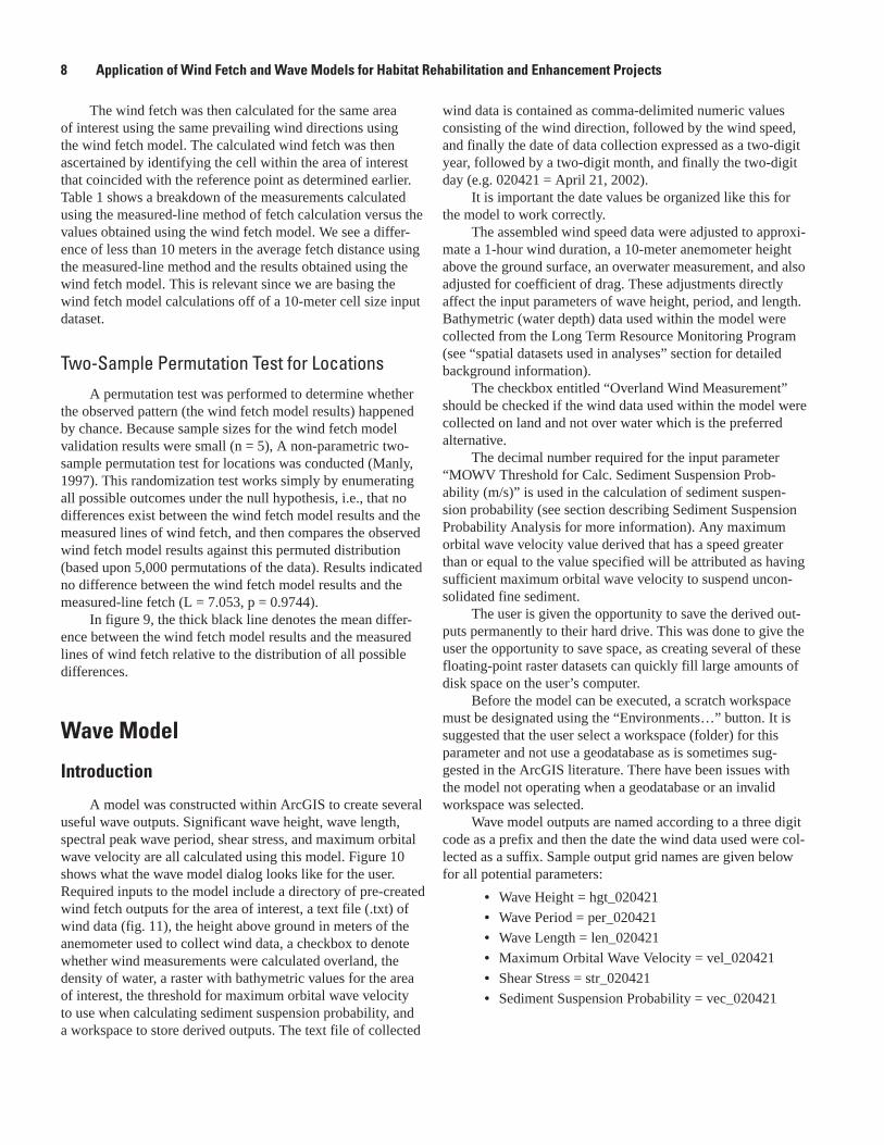
The units for this output are meters. The top-left frame of figure 13 displays an example output for wave height using wind fetch calculated from 300 degrees and a wind speed of 21 miles per hour for Capoli Slough HREP, management sce-nario 4. Areas within the HREP area of interest that are black denote land. The presence of “streaks” in this and the follow-ing figures are an unfortunate artifact of the stair-step nature of raster datasets. When polygons become thin (approximat-ing the raster’s cell size, in this example 10 meters), gaps are created in the island areas during the conversion to a raster dataset. When fetch is then calculated at certain angles, the fetch calculation is unimpeded by land. A possible resolution to this problem would be to further decrease cell-size to 5 or even 2 meters but then analysis time increases significantly.
Wave LengthThe wave length is the horizontal distance between two
identical points on two successive wave crests or two suc-cessive wave troughs (U.S. Army Corps of Engineers, 2002). Wave length measurements within the wave model are based upon linear wave theory. Linear wave theory is easy to apply and gives a reasonable approximation of wave characteristics for a wide range of wave parameters (U.S. Army Corps of Engineers, 2002). The assumptions made in developing the linear wave theory are
The fluid is homogeneous and incompressible; there-•fore, the density ρ is a constant.
Surface tension can be neglected.•
Coriolis Effect due to the Earth's rotation can be •neglected.
Pressure at the free surface is uniform and constant.•
The fluid is ideal or inviscid (lacks viscosity).•
The particular wave being considered does not interact •with any other water motions. The flow is irrotational so that water particles do not rotate (only normal forces are important and shearing forces are negligible).
The bed is a horizontal, fixed, impermeable boundary, •which implies that the vertical velocity at the bed is zero.
The wave amplitude is small and the waveform is •invariant in time and space.
Waves are plane or long-crested (two-dimensional).•
Wave length is calculated within the wave model accord-ing to the following formula:
L = g Tp2 / 2π
The units for this output are meters. The top-right frame of figure 13 displays an example output for wave length using wind fetch calculated from 300 degrees and a wind speed of 21 miles per hour for Capoli Slough HREP, management scenario 4.
Spectral Peak Wave PeriodThe time interval between the passage of two succes-
sive wave crests or troughs at a given point is the wave period (U.S. Army Corps of Engineers, 2002). Spectral peak wave period is calculated within the wave model according to the following formulae taken from the Coastal Engineering Manual (U.S. Army Corps of Engineers, 2002):
Tˆp =
2 * (xˆ)m2
Tp = (Tˆ
p * U*) / g
The units for this output are seconds. The middle-left frame of figure 13 displays an example
output for wave period using wind fetch calculated from 300 degrees and a wind speed of 21 miles per hour for Capoli Slough HREP, management scenario 4.
Maximum Orbital Wave VelocityAs waves begin to build, an orbital motion is created
in the water column resulting in a bottom velocity and shear stress (U.S. Army Corps of Engineers, 2006). This orbital wave velocity can be sufficient enough to suspend uncon-solidated sediments into the water column. In sufficiently deep water, the wave particle orbital velocity at the bottom is effectively zero and sediment particles on the bed do not expe-rience a force due to surface wave motion (Kraus, 1991). The maximum orbital wave velocity is calculated within the wave model according to the following formula (Kraus, 1991):
um = π H
m0 / (T
p sinh (2π d
f / L))
Maximum orbital wave velocity is based upon linear wave theory (see section describing wave length). The units for this output are meters per second. The middle-right frame of figure 13 displays an example output for maximum orbital wave velocity using wind fetch calculated from 300 degrees and a wind speed of 21 miles per hour for Capoli Slough HREP, management scenario 4.
Shear Stress Shear stress is the drag force created on the bed by the
fluid motion (Kraus, 1991). Shear stress at the bottom of the water column is understood to be an average over a wave period and is calculated within the wave model according to the following formula (Kraus, 1991):
τ = ρ f um
2 / 2
The units for this output are Newtons per square meter. The bottom-left of figure 13 displays an example output for shear stress using wind fetch calculated from 300 degrees and a wind speed of 21 miles per hour for Capoli Slough HREP, management scenario 4.
Figure 14 is a flowchart diagram depicting the relation-ships of the input and output parameters used to develop the wave models within the tool.
16 Application of Wind Fetch and Wave Models for Habitat Rehabilitation and Enhancement Projects
Wave Height
Wave Length
Wave Period
Maximum Orbital Wave Velocity
Shear Stress
High: 0.5
(Meters)
Low : 0.01
High : 9.4
(Meters)
Low : 0.1
High : 2.4
(Seconds)
Low : 0.2
High : 90
(Meters/Sec)
Low : 0
High : 130,284
(Newtons/Sq. Meter)
Low : 0
Capoli Slough HREP Area of Interest
Land (Scenario 4)
1,000Meters
Figure 13. Sample wave model outputs for scenario 4, Capoli Slough Habitat Rehabilitation and Enhancement Project.

St. Paul District Analyses 17
Figure 14. Diagram depicting relationships of input and output parameters used within the wave model.
St. Paul District Analyses
Study Areas
The study areas for these analyses are Capoli Slough and Harpers Slough HREPs in Navigation Pool 9 of the Upper Mississippi River System (UMRS; fig. 15). Both of these proposed HREPs are being designed to not only achieve goals and objectives related to the improvement of habitat but to also have a physical impact on riverine processes. Both projects intend to slow the loss of existing islands and to also restore islands that were lost.
“Islands reverse many of the effects of lock and dam construction. A new island essentially becomes the new natural levee, separating channel from flood-plain, reducing channel-floodplain connectivity, and increasing channel flow while decreasing the amount of floodplain flow. This increases the veloc-ity in adjacent channels increasing the erosion and
transport of sediment. Wind fetch and wave action is reduced in the vicinity of islands, reducing the resus-pension of bottom sediments, floodplain erosion, and shoreline erosion. In some cases, islands act primarily as wave barriers and don’t alter the river-wide distribution of flow. Islands reduce the supply of sediment to the floodplain potentially decreasing floodplain sediment deposition” (U.S. Army Corps of Engineers, 2006).
Capoli Slough Habitat Rehabilitation and Enhancement Project
Capoli Slough HREP is described in the USACE fact sheet as a side channel/island complex located on the Wiscon-sin side of the Mississippi River navigation channel in Pool 9, about five miles downstream of Lansing, Iowa. The site lies within the Upper Mississippi River National Wildlife and Fish Refuge (U.S. Army Corps of Engineers, n.d.a).

18 Application of Wind Fetch and Wave Models for Habitat Rehabilitation and Enhancement Projects
Many of the natural islands bordering the navigation channel have eroded, and many are disappearing. Erosion from wave action and main channel flows are reducing the size of the wetland complex, resulting in the loss of aquatic vegetation and the shallow protected habitats important for the survival of many species of fish and wildlife (U.S. Army Corps of Engineers, n.d.a).
The proposed project would restore islands to reduce fetch lengths. Breached areas would be stabilized using rock sills, and partial-closing structures would be constructed to reduce the effect of main channel flows. Material to restore the island complex would be dredged from the immediate vicin-ity to provide additional deepwater fish habitat benefits. It is estimated that the project would provide both fish and wildlife benefits by creating a “shadow” effect behind and downstream of the islands. About 600 acres of backwater habitat would be directly affected (U.S. Army Corps of Engineers, n.d.a).
Six specific habitat objectives were outlined in the Capoli Slough HREP Problem Appraisal Report (U.S. Army Corps of Engineers, 2001).
Increase the acreage of emergent vegetation and 1. floating-leafed vegetation by 10 percent over 2000 (LTRMP land cover) coverage.
Within the Capoli Slough complex, maintain Capoli 2. Slough and other well-defined running slough habi-tats and restore similar habitat where possible.
Maintain isolated wetlands and aquatic areas within 3. the Capoli Slough complex.
Maintain existing islands and increase the acreage of 4. island habitat.
Provide waterfowl and turtle nesting habitat within 5. or near the Capoli Slough complex.
Enhance and (or) develop protected off-channel 6. lacustrine fisheries habitat within the Capoli Slough complex, consistent with other habitat goals and objectives.
Figure 15. Location of Pool 9 Capoli Slough and Harpers Slough Habitat Rehabilitation and Enhancement Projects.
CO
UN
TY HW
Y N
WATERVILLE R
D
COUNTY
HWY C
COUNTYTRUNK
HWY A52
STATE HWY 249
STATEHWY 171COLU
MBUS RD
COUNTY HWY H
STATE
HWY 82
STA
TE H
WY
26
COUNTY
HWY A26
STATE HWY 82
STATE HWY 9
COUNTYHWY A52
STATE HW
Y 35COUNTY
HWY CB
STATE HW
Y 35
STATE
HWY
364
COUNTY HWY K
STATE HWY 56
CO
UN
TY HW
Y X52
STATE
HWY 9
Wisconsin
Iowa
Minnesota
Crawford
Vernon
Houston
Allamakee
0 4 82
Miles
IA
MN
WI
HREP Locations
Major Roadways
USFWS Refuge
UMRS Navigation Pool 9Land
Water
StatesCounties
Capoli Slough HREPHarpers Slough HREP
EXPLANATION

St. Paul District Analyses 19
Figure 16 gives a visual representation of the Capoli Slough HREP area using the 2000 LTRMP Land Cover/Land Use spatial data layer as a backdrop. The yellow Capoli Slough HREP area of interest polygon was created by buff-ering land areas affected by the HREP 500 meters. When interpreting the legend, features labeled “Added for Scenario 3”, for example, also include previous island designs from Scenarios 1 and 2 as well as existing land to create the com-plete Scenario 3 island design assemblage used in the models. Features are labeled according to USACE HREP planning maps.
Harpers Slough Habitat Rehabilitation and Enhancement Project
The Harpers Slough HREP is described in the USACE fact sheet as a 2,200-acre backwater area located primarily on the Iowa side of the Mississippi River in Pool 9, about 3 miles upstream of Lock and Dam 9. The site lies within the
Upper Mississippi River National Wildlife and Fish Refuge (U.S. Army Corps of Engineers, n.d.b).
The area is used heavily by tundra swans, Canada geese, puddle and diving ducks, black terns, nesting eagles, bit-terns, and cormorants and is also significant as a fish nursery area. Many of the islands in the area have been eroded or lost because of wave action and ice movement. This allows more turbulence in the backwater area, resulting in less productive habitat for fish and wildlife. Harpers Slough is one of the few remaining areas in lower Pool 9 where high quality habitat could be maintained (U.S. Army Corps of Engineers, n.d.b).
The proposed project would restore about 25,000 feet of islands at the upper portion of the area using material from the backwater and near the main channel. About 8,000 feet of islands in the lower portion of the area would be stabilized. The project would slow the loss of existing islands, reduce the flow of sediment-laden water into the backwaters, and increase the diversity of land and shoreline habitats (U.S. Army Corps of Engineers, n.d.b).
Island F
Island E
Island B
Island I
Island H
Island A
Island D
Island C
Island K3
Island K2
Island G
Island K
Island 2
Island 1Island 3
Island 4
Island 8
Island 6
Island 7
Island 9
Island 11Island 10
EmergentWetland K
EmergentWetland G
EmergentWetland I
EmergentWetland C
Rock MoundWetland E
Rock MoundWetland C
CobbleLiner A
CobbleLiner B
Closure A
Closure B
Closure E
Closure D
Closure C
658
657
0 500 1,000250
Meters
Background image is a USGSNational Elevation Dataset
Revised 2000 LTRMP Land Cover/Land Use
Existing LandWater
Added for Scenario 4Added for Scenario 3Added for Scenario 2Added for Scenario 1
COE Sail Line
River Miles
Capoli Slough HREP Area of Interest
EXPLANATION
Figure 16. Capoli Slough Habitat Rehabilitation and Enhancement Project with feature labels.
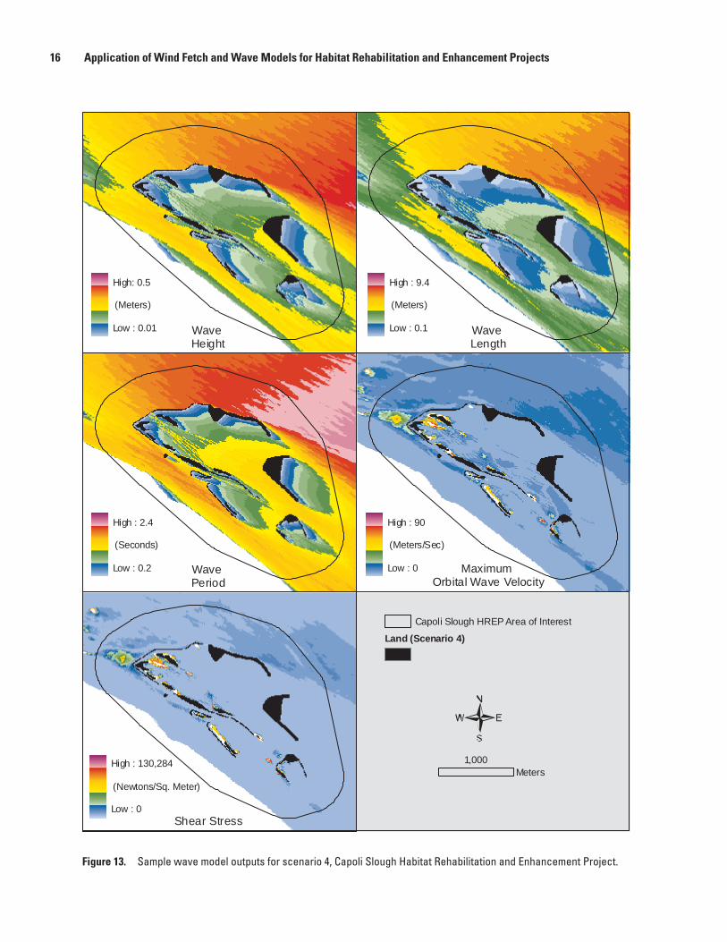
20 Application of Wind Fetch and Wave Models for Habitat Rehabilitation and Enhancement Projects
There are four goals outlined within the Harpers Slough rough draft Definite Project Report (U.S. Army Corps of Engineers, 2005).
Maintain and (or) enhance habitat in the Harpers 1. Slough backwater area for migratory birds.
Create habitat for migratory and resident vertebrates 2. with emphasis on marsh and shorebirds, bald eagles, and turtles.
Improve and maintain habitat conditions for backwa-3. ter fish species.
Enhance secondary and main channel border habitat 4. for riverine fish species and mussels.
Figure 17 gives a visual representation of the Harpers Slough HREP area using the 2000 LTRMP Land Cover/Land Use spatial data layer as a backdrop. The yellow Harpers Slough HREP area of interest polygon was created by buffer-ing land areas affected by the HREP 500 meters. When inter-preting the legend, features labeled “Added for Scenario 3,” for example, also include previous island designs from Sce-narios 1 and 2 as well as existing land to create the complete Scenario 3 island design assemblage used in the models. Fea-tures are labeled according to USACE HREP planning maps.
Island I1
SeedIsland
Island X1
Island X3
Island A2
SeedIsland
Island D
Island UV
Island I2
Island X1
Island P
Island X2
Island A3
Island I3
Island RS
EmergentWetland
EmergentWetland
EmergentWetland
IsolatedWetland
Off-shoreRock
Mound A1
Off-shoreRock
Mound K
RockSill X1
RockSill A3
RockSill I3
RockSill P
RockSill I
655
654
653
652
6510 500 1,000250
Meters
Background image is a USGSNational Elevation Dataset
Revised 2000 LTRMP Land Cover/Land Use
Harpers Slough HREP Area of Interest
Existing LandWater
Added for Scenario 4Added for Scenario 3Added for Scenario 2Added for Scenario 1
COE Sail Line
River Miles
EXPLANATION
Figure 17. Harpers Slough Habitat Rehabilitation and Enhancement Project with feature labels.

St. Paul District Analyses 21
Weighted Wind Fetch Analysis
Land Raster Input DataThe 2000 land cover data created by the LTRMP were
used to depict the land/water interface used within the wind fetch model for this particular analysis (see “spatial datasets used in analyses” section for detailed background informa-tion). Some details in existing land/water morphology were updated using existing island polygons supplied by the USACE for Capoli Slough HREP. Also, an existing bar-rier island was digitized and included into all management scenarios for Harpers Slough HREP (fig. 18). This island was created just to the west of river mile 654.
Island design scenarios were provided by the St. Paul District, U.S. Army Corps of Engineers and incorporated into the 2000 LTRMP land cover. These land/water datasets pro-vided the base layers used to calculate fetch. To be used within the model, these land/water datasets were given a new field. This field was attributed so all land polygons were “1” and all water polygons were attributed as “0.” The polygons were then converted from their native polygonal (shapefile) format into an ESRI raster format (Grid) to be used in the model. The field that was added was used to assign values to the output raster.
This was accomplished in ArcGIS 9.2 using the “Feature to Raster” tool. The output rasters have a cell size of 10 meters.
The specific island configuration scenario to be used within the wind fetch model is designated using the “Land Raster” control on the wind fetch model dialog window.
Wind Direction Input DataWind direction data used within the wind fetch model
were collected from the National Oceanic and Atmospheric Administration, National Climatic Data Center (NCDC) (http://www7.ncdc.noaa.gov/IPS/LCDPubs?action=getstate&LCD=hardcode). The specific wind parameter used was the maximum 2-minute average wind direction. Wind data used in this analysis were collected only during the growing seasons (April–July) from 1998 to 2007. All daily wind data were used regardless of collected wind speed. Wind data for significant events could be selected manually to represent wind speeds and directions of primary concern. Only April data were available for 2007 at the time of analysis. Figure 19 gives an example of NCDC local climatological data for May 2006 from the La Crosse Municipal Airport. This was the closest data collection location to the study areas of Capoli and Harpers Slough HREPs.
Figure 18. Location of revised island addition to Harpers Slough Habitat Rehabilitation and Enhancement Project area.

22 Application of Wind Fetch and Wave Models for Habitat Rehabilitation and Enhancement Projects
Figu
re 1
9.
Nat
iona
l Clim
atic
Dat
a Ce
nter
, Loc
al C
limat
olog
ical
Dat
a su
mm
ary
shee
t.
St. Paul District Analyses 23
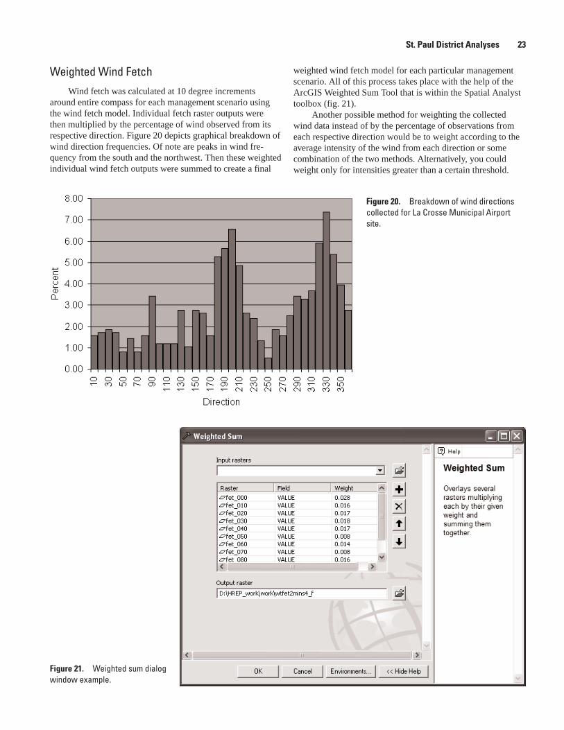
Weighted Wind FetchWind fetch was calculated at 10 degree increments
around entire compass for each management scenario using the wind fetch model. Individual fetch raster outputs were then multiplied by the percentage of wind observed from its respective direction. Figure 20 depicts graphical breakdown of wind direction frequencies. Of note are peaks in wind fre-quency from the south and the northwest. Then these weighted individual wind fetch outputs were summed to create a final
weighted wind fetch model for each particular management scenario. All of this process takes place with the help of the ArcGIS Weighted Sum Tool that is within the Spatial Analyst toolbox (fig. 21).
Another possible method for weighting the collected wind data instead of by the percentage of observations from each respective direction would be to weight according to the average intensity of the wind from each direction or some combination of the two methods. Alternatively, you could weight only for intensities greater than a certain threshold.
Figure 20. Breakdown of wind directions collected for La Crosse Municipal Airport site.
Figure 21. Weighted sum dialog window example.

24 Application of Wind Fetch and Wave Models for Habitat Rehabilitation and Enhancement Projects
Analysis ResultsWeighted wind fetch was calculated for UMRS Pool 9
for each potential management scenario; No-Action, Existing Conditions, Scenario 1, Scenario 2, Scenario 3, and Sce-nario 4.
Figures 22 and 23 display the results of the weighted wind fetch analysis for each management scenario, for the Capoli Slough HREP and Harpers Slough HREP, respectively.
Figure 24 depicts the difference in weighted wind fetch in meters from the existing conditions management scenario to scenarios 1, 2, 3, and 4 for Capoli Slough HREP.
Figure 25 shows the numerical difference in weighted wind fetch from the existing conditions management scenario to scenarios 1, 2, 3, and 4 for Capoli Slough HREP.
Figure 26 depicts the difference in weighted wind fetch in meters from the existing conditions management scenario to scenarios 1, 2, 3, and 4 for Harpers Slough HREP.
Figure 27 shows the numerical difference in weighted wind fetch from the existing conditions management scenario to scenarios 1, 2, 3, and 4 for Harpers Slough HREP.
DiscussionUsing this weighted fetch analysis approach it is pos-
sible to quantify the amount of wind fetch for each of the separate island design management scenarios and compare how the addition of potential island structures may affect wind fetch. This approach took into account historical wind data. Site-specific wind data would have been preferred but this was unavailable. The ability to decrease wind fetch within the HREP locations would benefit these sites by lessening the forces applied due to wave energy and thereby decreas-ing turbidity. With the addition of features for each manage-ment scenario progressing from 1 to 4 we see decreases in the amount of weighted wind fetch within both study areas. The next step would be to perform a cost-benefit analysis to ascer-tain whether the monetary costs of the additional features with each successive island design are worth the modeled ecologi-cal benefits.
Sediment Suspension Probability Analysis
Many factors affect aquatic plant growth. These may include site-characteristic changes in climate, water tem-perature, water transparency, pH, and oxygen effects on CO
2
assimilation rate at light saturation, wintering strategies, graz-ing and mechanical control (removal of shoot biomass), and of latitude (Best and Boyd, 1999). According to Kreiling and others, 2007, “light, rather than nutrients, was the main abiotic factor associated with the peak Vallisneria shoot biomass in Pool 8.” Wave action has a direct effect on water transparency. When sediments are suspended by wave action, it causes an increase in water turbidity. High turbidity can reduce aquatic plant growth by decreasing water transparency, thus limiting light penetration.
The sediment suspension probability analysis developed for Capoli and Harpers Slough HREPs involved executing the wave models to calculate maximum orbital wave velocity (MOWV) outputs for each potential management scenario and applying these MOWV values to predict sediment suspension probabilities. According to Coops and others, 1991, “maxi-mal wave heights and orbital velocities were concluded to be key factors in the decreased growth rates of plants at exposed sites.”
The MOWV was calculated once daily over the growing season (April through July) encompassing the 6-year period between 2002 and 2007 (n = 640 days). Only April data were available for the year 2007 at the time analysis was executed. The MOWV of 0.10 meters per second was then selected to represent velocities required to suspend fine unconsolidated sediments (Håkanson and Jansson, 1983).
Bathymetric data used in the wave model equations were obtained from the Long Term Resource Monitoring Program (see “spatial datasets used in analyses” section for detailed background information). The bathymetric data had to be modified when calculating the MOWV for the “No Action” management scenario. All island areas that were predicted to be lost in that scenario were given the lowest water depth for those areas, in this example 0.01 meters (1 centimeter).

St. Paul District Analyses 25
No-Action
2 oiranecS1 oiranecS
4 oiranecS3 oiranecS
ExistingConditions
1,000
Meters
Weighted Wind Fetch (Meters)01 - 100101 - 200201 - 300301 - 400401 - 500501 - 600
1,801 - 1,9001,901 - 2,0002,001 - 2,1002,101 - 2,2002,201 - 2,3002,301 - 2,400
2,401 - 2,5002,501 - 2,6002,601 - 2,7002,701 - 2,8002,801 - 2,9002,901 - 3,000> 3,000
1,201 - 1,3001,301 - 1,4001,401 - 1,5001,501 - 1,6001,601 - 1,7001,701 - 1,800
HREP Area of Interest
601 - 700701 - 800801 - 900901 - 1,0001,001 - 1,1001,101 - 1,200
Land
Figure 22. Weighted wind fetch results for the Capoli Slough Habitat Rehabilitation and Enhancement Project.

26 Application of Wind Fetch and Wave Models for Habitat Rehabilitation and Enhancement Projects
No-Action
2 oiranecS1 oiranecS
4 oiranecS3 oiranecS
ExistingConditions
2,000
Meters
Weighted Wind Fetch (Meters)01 - 100101 - 200201 - 300301 - 400401 - 500501 - 600
1,801 - 1,9001,901 - 2,0002,001 - 2,1002,101 - 2,2002,201 - 2,3002,301 - 2,400
2,401 - 2,5002,501 - 2,6002,601 - 2,7002,701 - 2,8002,801 - 2,9002,901 - 3,000> 3,000
1,201 - 1,3001,301 - 1,4001,401 - 1,5001,501 - 1,6001,601 - 1,7001,701 - 1,800
HREP Area of Interest
601 - 700701 - 800801 - 900901 - 1,0001,001 - 1,1001,101 - 1,200
Land
Figure 23. Weighted wind fetch results for the Harpers Slough Habitat Rehabilitation and Enhancement Project.

St. Paul District Analyses 27
Scenario 1
4 oiranecS3 oiranecS
Scenario 2
1,000
Meters
Weighted Wind Fetch (Meters)01 - 100101 - 200201 - 300301 - 400401 - 500501 - 600
1,801 - 1,9001,901 - 2,0002,001 - 2,1002,101 - 2,2002,201 - 2,3002,301 - 2,400
2,401 - 2,5002,501 - 2,6002,601 - 2,7002,701 - 2,8002,801 - 2,9002,901 - 3,000> 3,000
1,201 - 1,3001,301 - 1,4001,401 - 1,5001,501 - 1,6001,601 - 1,7001,701 - 1,800
HREP Area of Interest
601 - 700701 - 800801 - 900901 - 1,0001,001 - 1,1001,101 - 1,200
Land
Figure 24. Difference in weighted wind fetch from the existing conditions management scenario to scenarios 1, 2, 3, and 4 for the Capoli Slough Habitat Rehabilitation and Enhancement Project.
Figure 25. Numerical difference in weighted wind fetch from the existing conditions management scenario to scenarios 1, 2, 3, and 4 for the Capoli Slough Habitat Rehabilitation and Enhancement Project.

28 Application of Wind Fetch and Wave Models for Habitat Rehabilitation and Enhancement Projects
Scenario 1
4 oiranecS3 oiranecS
Scenario 2
2,000
Meters
Weighted Wind Fetch (Meters)01 - 100101 - 200201 - 300301 - 400401 - 500501 - 600
1,801 - 1,9001,901 - 2,0002,001 - 2,1002,101 - 2,2002,201 - 2,3002,301 - 2,400
2,401 - 2,5002,501 - 2,6002,601 - 2,7002,701 - 2,8002,801 - 2,9002,901 - 3,000> 3,000
1,201 - 1,3001,301 - 1,4001,401 - 1,5001,501 - 1,6001,601 - 1,7001,701 - 1,800
HREP Area of Interest
601 - 700701 - 800801 - 900901 - 1,0001,001 - 1,1001,101 - 1,200
Land
Figure 27. Numerical difference in weighted wind fetch from the existing conditions management scenario to scenarios 1, 2, 3, and 4 for the Harpers Slough Habitat Rehabilitation and Enhancement Project.
Figure 26. Difference in weighted wind fetch from the existing conditions management scenario to scenarios 1, 2, 3, and 4 for the Harpers Slough Habitat Rehabilitation and Enhancement Project.

St. Paul District Analyses 29
The next step in the analysis involved reclassifying areas within the output MOWV raster that had MOWV values >= 0.10 meters per second with a “1” value and reclassify-ing areas within the output MOWV raster that had MOWV < 0.10 meters per second with a “0” value. This was done for all 640 raster outputs. Next, these individual reclassified raster datasets were merged together into one raster dataset and the values divided by the total number of days (640) to get a percentage of days that MOWV was at least 0.10 meters per second for each individual raster cell. This value then repre-sents the probability to suspend fine unconsolidated particles. Figure 28 gives a graphical illustration of the process used to create the final outputs using four hypothetical raster datasets as an example.
Analysis ResultsSediment suspension probability was calculated for
UMRS Pool 9 for each potential management scenario: No-Action, Existing Conditions, Scenario 1, Scenario 2, Scenario 3, and Scenario 4.
Figures 29 and 30 display the results of the sediment suspension probability analysis for each management scenario, for the Capoli Slough and Harpers Slough HREP, respectively.
Figure 31 depicts the difference in sediment suspension probability from the existing conditions management scenario to scenarios 1, 2, 3, and 4 for Capoli Slough HREP.
Figure 32 shows the numerical difference in sediment suspension probability from the existing conditions manage-ment scenario to scenarios 1, 2, 3, and 4 for Capoli Slough HREP.
Figure 33 depicts the difference in sediment suspension probability from the existing conditions management scenario to scenarios 1, 2, 3, and 4 for Harpers Slough HREP.
Figure 34 shows the numerical difference in sediment suspension probability from the existing conditions manage-ment scenario to scenarios 1, 2, 3, and 4 for Harpers Slough HREP.
Figure 28. Diagram explaining process for calculating percent of days capable of suspending sediments.

30 Application of Wind Fetch and Wave Models for Habitat Rehabilitation and Enhancement Projects
No-Action
2 oiranecS1 oiranecS
4 oiranecS3 oiranecS
ExistingConditions
1,000
Meters
Sediment Suspension Probability (Percentage of Days)
HREP Area of InterestLand
0
0.1 - 5
5.1 - 10
10.1 - 15
15.1 - 20 40.1 - 45
20.1 - 25
25.1 - 30
30.1 - 35
35.1 - 40
45.1 - 50
50.1 - 55
55.1 - 60
60.1 - 65
65.1 - 70
70.1 - 75
75.1 - 80
80.1 - 85
85.1 - 90
90.1 - 95
95.1 - 100
Figure 29. Sediment suspension probability results for the Capoli Slough Habitat Rehabilitation and Enhancement Project.

St. Paul District Analyses 31
No-Action
2 oiranecS1 oiranecS
4 oiranecS3 oiranecS
ExistingConditions
2,000
Meters
Sediment Suspension Probability (Percentage of Days)
HREP Area of InterestLand
0
0.1 - 5
5.1 - 10
10.1 - 15
15.1 - 20 40.1 - 45
20.1 - 25
25.1 - 30
30.1 - 35
35.1 - 40
45.1 - 50
50.1 - 55
55.1 - 60
60.1 - 65
65.1 - 70
70.1 - 75
75.1 - 80
80.1 - 85
85.1 - 90
90.1 - 95
95.1 - 100
Figure 30. Sediment suspension probability results for the Harpers Slough Habitat Rehabilitation and Enhancement Project.

32 Application of Wind Fetch and Wave Models for Habitat Rehabilitation and Enhancement Projects
Scenario 1
4 oiranecS3 oiranecS
Scenario 2
1,000
Meters
Sediment Suspension Probability (Percentage of Days)
HREP Area of InterestLand
0
0.1 - 5
5.1 - 10
10.1 - 15
15.1 - 20 40.1 - 45
20.1 - 25
25.1 - 30
30.1 - 35
35.1 - 40
45.1 - 50
50.1 - 55
55.1 - 60
60.1 - 65
65.1 - 70
70.1 - 75
75.1 - 80
80.1 - 85
85.1 - 90
90.1 - 95
95.1 - 100
Figure 31. Difference in sediment suspension probability from the existing conditions management scenario to scenarios 1, 2, 3, and 4 for the Capoli Slough Habitat Rehabilitation and Enhancement Project.
Figure 32. Numerical difference in sediment suspension probability from the existing conditions management scenario to scenarios 1, 2, 3, and 4 for the Capoli Slough Habitat Rehabilitation and Enhancement Project.

St. Paul District Analyses 33
Scenario 1
4 oiranecS3 oiranecS
Scenario 2
2,000
Meters
Sediment Suspension Probability (Percentage of Days)
HREP Area of InterestLand
0
0.1 - 5
5.1 - 10
10.1 - 15
15.1 - 20 40.1 - 45
20.1 - 25
25.1 - 30
30.1 - 35
35.1 - 40
45.1 - 50
50.1 - 55
55.1 - 60
60.1 - 65
65.1 - 70
70.1 - 75
75.1 - 80
80.1 - 85
85.1 - 90
90.1 - 95
95.1 - 100
Figure 33. Difference in sediment suspension probability from the existing conditions management scenario to scenarios 1, 2, 3, and 4 for the Harpers Slough Habitat Rehabilitation and Enhancement Project.
Figure 34. Numerical difference in sediment suspension probability from the existing conditions management scenario to scenarios 1, 2, 3, and 4 for the Harpers Slough Habitat Rehabilitation and Enhancement Project.

34 Application of Wind Fetch and Wave Models for Habitat Rehabilitation and Enhancement Projects
DiscussionThis analysis provides a simplistic approach to forecast-
ing wave effects on the suspension of fine unconsolidated sediment particles. Based upon this approach, it is possible to depict changes in sediment suspension probability for several potential island construction scenarios at the identified HREP areas both with maps and summary charts. By decreasing the potential for sediments to be suspended, there would be a decrease in turbidity. Decreasing turbidity would increase light penetration and, therefore, create conditions more conducive to aquatic plant growth. This approach took into account his-torical wind data. Site-specific wind data would have been pre-ferred but this was unavailable. With the addition of features for each management scenario progressing from 1 to 4, we see decreases in the percentage of days with MOWV capable of suspending fine unconsolidated particles within both study
areas. Likewise, with the weighted wind fetch analysis, the next step would be to perform a cost-benefit analysis to ascer-tain whether the monetary costs of the additional features with each successive island design are worth the modeled ecologi-cal benefits.
St. Louis District Analysis
Study Area
Swan Lake Habitat Rehabilitation and Enhancement Project
The study area for this analysis was Swan Lake HREP which is located near the confluence of the Illinois and Missis-sippi Rivers within the UMRS near Brussels, Illinois (fig. 35).
Figure 35. Location of Swan Lake Habitat Rehabilitation and Enhancement Project.
Illinois
Missouri
Jersey
Calhoun
Greene
St.Charles
Background image is the USGS National Elevation Dataset.
0 4 82
Miles
Two R
ivers
Nation
al
Wild
life R
efuge
Big Mud
dy N
ation
al Fish
and W
ildlife
Refu
ge
ILIA
MOHREP Location
Swan Lake HREP Area
LTRMP Land Cover
LandWater
USFWS Refuge
StatesCounties
EXPLANATION

St. Louis District Analysis 35
Swan Lake HREP is described in the 1993 USACE defi-nite project report as being located adjacent to the west bank of the Illinois River between river miles 5 and 13. The imme-diate project area includes 2,900-acre Swan Lake, 200-acre Fuller Lake, and approximately 950 acres of bottomland forest and 550 acres of cropland surrounding these lakes (totaling 4,600 acres). Also included in the project area is the local watershed adjacent to Swan Lake’s west shore (U.S. Army Corps of Engineers, 1993).
Management of the project area is divided. Fuller Lake and the uppermost 300 acres of Swan Lake are managed for the USFWS by the Illinois Department of Conserva-tion (IDOC). The remaining 2,600 acres of Swan Lake are managed directly by the USFWS as part of the Mark Twain National Wildlife Refuge. East of the project area is the Stump Lake HREP and to the southwest, the project abuts the Cal-houn Point HREP area. Collectively, these three areas com-prise about one-fourth of all wetland and deepwater habitats to be found in the lower 80 miles of the Illinois River valley, and they form an integral component of a nationally significant ecosystem (U.S. Army Corps of Engineers, 1993).
Swan Lake is vitally important as habitat for both water-fowl and fish. The lake lies within a portion of the Missis-sippi Flyway designated as an area of major concern under the North American Waterfowl Management Plan. Ongoing
habitat loss has reduced the value of this area for waterfowl as a migration feeding and resting area. From a fisheries stand-point, the lake furnishes a major portion of the region’s avail-able spawning, rearing, and wintering habitat. The lake is open to both sport and commercial fishing. Biologists are concerned that a continuing loss of river backwater habitat could result in a future reduction in fish abundance and diversity (U.S. Army Corps of Engineers, 1993).
Weighted Wind Fetch Analysis
Land Raster Input DataThe 2000 land cover data created by the LTRMP were
used to depict the land/water interface used within the wind fetch model for this particular analysis (see “spatial dataset used in analysis” section for detailed background information). A line of human-made island structures that exist between the northwest and southeast sections of the lower pool of the Swan Lake HREP were added to the base 2000 land/water dataset (fig. 36). These islands will have an effect on wind fetch so it was deemed essential to include in the following island design scenarios.
Figure 36. Location of revised island addition to Swan Lake Habitat Rehabilitation and Enhancement Project area.

36 Application of Wind Fetch and Wave Models for Habitat Rehabilitation and Enhancement Projects
U.S. Fish and Wildlife Service Sample Island Design
Figure 37 gives a visual representation of the Swan Lake HREP area and USFWS sample islands using 2006 USDA National Agriculture Imagery Program aerial photography as a backdrop. The yellow Swan Lake HREP area of interest polygon was created by selecting the polygons identified as “water” in the 2000 LTRMP land cover/land use spatial data layer within the lower pool of the Swan Lake HREP area.
A sample island design was created by personnel at Two Rivers National Wildlife Refuge to help decrease wind fetch within Swan Lake. The USFWS staff at the refuge were given a map of current weighted wind fetch to help place the islands. These islands are displayed in purple in figure 37 and have a total acreage of 12.395 acres. Features are labeled according to randomly generated numbers preceded by an “A” (northwest section of Swan Lake HREP area) or a “B” (southeast section of Swan Lake HREP area) to differentiate the separate por-tions of the Swan Lake area of interest.
0 500 1,000250
Meters
Background image is a 2006USDA National AgricultureImagery Program Aerial Photo
Swan Lake HREP Area of Interest
USFWS Proposed Island DesignIllinois River
A1
A2
B1 B2
Figure 37. Swan Lake Habitat Rehabilitation and Enhancement Project with U.S. Fish and Wildlife Service proposed islands labeled.
U.S. Army Corps of Engineers Sample Island Design
Figure 38 gives a visual representation of the Swan Lake HREP area using 2006 USDA National Agriculture Imagery Program aerial photography as a backdrop and also includes a sample island design created by staff at the USACE St. Louis District office to impede wind fetch. The USACE staff at the district were given a map of current weighted wind fetch to help place the islands. These islands are displayed in purple
in figure 38 and have a total area of 40.085 acres. Features are labeled according to randomly generated numbers preceded by an “A” or a “B” to differentiate the separate portions of the Swan Lake area of interest.
These land/water datasets provided the base layers used to calculate fetch. To be used within the model, these land/water datasets were given a new field. This field was attributed so all land polygons were “1” and all water polygons were attributed as “0.” The polygons were then converted from their native polygonal (shapefile) format into an ESRI raster format

St. Louis District Analysis 37
(Grid) to be used in the model. The field added was used to assign values to the output raster. This was accomplished in ArcGIS 9.2 using the “Feature to Raster” tool. The output rasters have a cell size of 10 meters.
The specific island configuration scenario to be used within the wind fetch model is designated using the “Land Raster” control on the wind fetch model dialog window.
Wind Direction Input DataWind direction data used within the wind fetch model
were collected from the National Oceanic and Atmospheric Administration, National Climatic Data Center (NCDC) (http://www7.ncdc.noaa.gov/IPS/LCDPubs?action=getstate&LCD=hardcode). The specific wind parameter used was the maximum 2-minute average wind direction. Wind data used in this analysis was collected only during the growing seasons (April–July) from 1998 to 2007. All daily wind data were used regardless of collected wind speed. Wind data for significant events could be selected manually to represent wind speeds and directions of primary concern. Only April data were avail-
able for 2007 at the time of analysis. Figure 39 gives an exam-ple of NCDC local climatological data for April 2007 from the Lambert–St. Louis International Airport. This was the closest NCDC data collection location to Swan Lake HREP.
Weighted Wind FetchWind fetch was calculated at 10-degree increments
around entire compass for each management scenario using the wind fetch model. Wind fetch was calculated using the SPM calculation method. Individual fetch raster outputs were then multiplied by the percentage of wind observed from its respective direction. Figure 40 depicts graphical breakdown of wind direction frequencies. Of note are peaks in wind frequency from the south and the northwest. These weighted individual wind fetch outputs were summed to create a final weighted wind fetch model for each particular management scenario. All of this process takes place with the help of the ArcGIS Weighted Sum Tool that is within the Spatial Analyst toolbox (fig. 41).
B7B8
B9
B6
B5B4B3
B2B1
A6A5
A4
A3A2
A1
0 500 1,000250
Meters
Background image is a 2006USDA National AgricultureImagery Program Aerial Photo
Swan Lake HREP Area of Interest
USACE Proposed Island DesignIllinois River
Figure 38. Swan Lake Habitat Rehabilitation and Enhancement Project with U.S. Army Corps of Engineers proposed islands labeled.
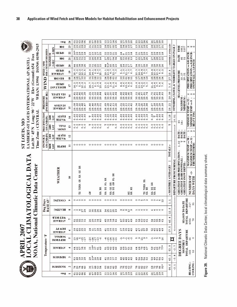
38 Application of Wind Fetch and Wave Models for Habitat Rehabilitation and Enhancement Projects
Figu
re 3
9.
Nat
iona
l Clim
atic
Dat
a Ce
nter
, loc
al c
limat
olog
ical
dat
a su
mm
ary
shee
t.
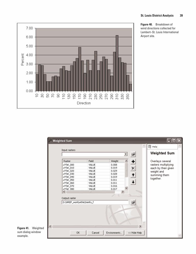
St. Louis District Analysis 39
Figure 40. Breakdown of wind directions collected for Lambert–St. Louis International Airport site.
Figure 41. Weighted sum dialog window example.

40 Application of Wind Fetch and Wave Models for Habitat Rehabilitation and Enhancement Projects
Another possible method for weighting the collected wind data instead of by the percentage of observations from each respective direction would be to weight according to the average intensity of the wind from each direction or some combination of the two methods. Alternatively, you could weight only for intensities greater than a certain threshold.
Analysis ResultsWeighted wind fetch was calculated for Swan Lake
HREP for each potential management scenario: Existing Con-ditions, USFWS Island Design, and USACE Island Design.
The top-left frame of figure 42 displays the results of the weighted wind fetch analysis for the existing conditions man-agement scenario, for the Swan Lake HREP. The middle-left frame of figure 42 displays the weighted wind fetch results for the USFWS Island Design, and the bottom-left frame of fig-ure 42 displays the difference in weighted fetch from the exist-ing conditions scenario to the island design scenario proposed by the USFWS. The middle-right frame of figure 42 displays the weighted wind fetch results for the USACE Island Design, and the bottom-right frame of figure 42 displays the difference in weighted fetch from the existing conditions scenario to the island design scenario proposed by the USACE.
Figure 43 displays the percent decrease in total weighted fetch between existing conditions and the USFWS proposed island design for Swan Lake HREP.
Figure 44 displays the percent decrease in total weighted fetch between existing conditions and the USACE proposed island design for Swan Lake HREP.
DiscussionUsing this weighted fetch analysis approach, it is pos-
sible to quantify the amount of wind fetch for each of the separate island design management scenarios and compare how the addition of potential island structures may affect wind fetch. This approach took into account historical wind data. Site-specific wind data would have been preferred but this was unavailable. The ability to decrease wind fetch within the HREP locations would benefit these sites by lessening the forces applied due to wave energy and thereby decreas-ing turbidity. With the addition of features for the USFWS and USACE management scenarios, we see decreases in the amount of weighted wind fetch within the Swan Lake HREP area. The next step would be to perform a cost-benefit analysis to ascertain whether the monetary costs of the proposed fea-tures with each island design are worth the modeled ecological benefits.
Spatial Datasets Used in AnalysesLong Term Resource Monitoring Program 2000 Land Cover/Land Use Data for the Upper Mississippi River System
OriginatorU.S. Geological Survey Upper Midwest Environmental
Sciences Center Long Term Resource Monitoring Program
AbstractThe UMESC created high-resolution land cover/use
data sets for the UMRS from 1:24,000-scale color infrared aerial photographs collected in 2000. The photographs were interpreted using a minimum mapping unit of 1-hectare and 10-percent minimum vegetation cover. The photographs were interpreted to delineate land cover/land use, percent vegeta-tion cover, tree height, and hydrology regime. The geographic extent of the UMRS is the Mississippi River from Cairo, Illinois, to Minneapolis, Minnesota, and the Illinois River from its confluence with the Mississippi near Grafton, Illinois, to Lake Michigan.
Online Linkagehttp://www.umesc.usgs.gov/data_library/land_cover_
use/2000_lcu_umesc.html
Long Term Resource Monitoring Program Bathymetric Data for the Upper Mississippi and Illinois Rivers
OriginatorU.S. Geological Survey Upper Midwest Environmental
Sciences Center Long Term Resource Monitoring Program
AbstractWater depth is an important feature of aquatic systems.
On the UMRS, water depth data are important for describing the physical template of the system and monitoring changes in the template caused by sedimentation. Although limited point or transect sampling of water depth can provide valuable information on habitat character in the UMRS as a whole, the generation of bathymetric surfaces are critical for conducting spatial inventories of the aquatic habitat. The maps are also useful for detecting bed elevation changes in a spatial manner as opposed to the more common method of measuring changes along transects. The UMESC has been collecting bathymetric data within the UMRS since 1989 in conjunction with the LTRMP.
Online Linkagehttp://www.umesc.er.usgs.gov/aquatic/bathymetry/
download.html

St. Louis District Analysis 41
Weighted Wind FetchExisting Conditions
Weighted Wind FetchUSFWS Island Design
Weighted Wind FetchUSACE Island Design
Difference in WeightedWind Fetch Between Existing Conditions and USFWS Island Design
Difference in WeightedWind Fetch Between Existing Conditions and USACE Island Design
1,000Meters
1,000Meters
1,000Meters
1,000Meters
Weighted Wind FetchMeters
00.1 - 4040.1 - 8080.1 - 120120.1 - 160160.1 - 200200.1 - 240240.1 - 280280.1 - 320320.1 - 360360.1 - 400400.1 - 440440.1 - 480
480.1 - 520520.1 - 560560.1 - 600600.1 - 640640.1 - 680680.1 - 720720.1 - 760760.1 - 800800.1 - 840840.1 - 880880.1 - 920920.1 - 960960.1 - 1,000> 1,000Land1,000
Meters
Figure 42. Results of weighted wind fetch analysis for Swan Lake Habitat Rehabilitation and Enhancement Project.

42 Application of Wind Fetch and Wave Models for Habitat Rehabilitation and Enhancement Projects
Figure 43. Percent decrease in total weighted fetch between existing conditions and U.S. Fish and Wildlife Service proposed island design for Swan Lake Habitat Rehabilitation and Enhancement Project.
Figure 44. Percent decrease in total weighted fetch between existing conditions and U.S. Army Corps of Engineers proposed island design for Swan Lake Habitat Rehabilitation and Enhancement Project.

References Cited 43
AcknowledgmentsWe thank Michael Walker and Jon Hendrickson,
U.S. Army Corps of Engineers, St. Paul District and John Mabery, U.S. Fish and Wildlife Service, Two Rivers National Wildlife Refuge for their assistance with this project. We thank Dr. Wayne Thogmartin for his assistance in the statistical validation of the wind fetch model. This report also was made measurably better by the comments of reviewers.
References Cited
Best, E.P.H., and Boyd, W.A., 1999, A simulation model for growth of the submersed aquatic macrophyte Myriophyl-lum spicatum L.: Vicksburg, Miss., U.S. Army Engineer Research and Development Center, Technical Report A–99–3.
Chamberlin, F., 1994, Wind-generated waves in navigation pools, in U.S. Army Corps of Engineers, St. Paul, Minn., for the National Biological Service, Environmental Manage-ment Technical Center, Onalaska, Wis.: December 1994, LTRMP 94-S001, 16 p. (NTIS #PB95–209532)
Coops, H., Boeters, R., and Smit, H., 1991, Direct and indirect effects of wave attack on helophytes: Aquat. Bot. 41:333–352.
Finlayson, D., 2005, Puget Sound Fetch: Seattle, Wash., University of Washington, School of Oceanography, accessed October 16, 2007, at URL http://david.p.finlayson.googlepages.com/pugetsoundfetch
Ford, D.E., and Stefan, H.G., 1980, Thermal predictions using integral energy model: Journal of the Hydraulics Division, v. 106, no. HY1.
Håkanson, L., and Jansson, M., 1983, Principles of lake sedimentology (2d ed.): New Jersey, The Blackburn Press, 316 p.
Kraus, N., 1991, Class notes for coastal sediment processes: Texas A&M University and Waterways Experiment Station Graduate Institute, OCEN 682, June 5 to August 9, 1991.
Kreiling, R.M., Yin, Y., and Gerber, D.T., 2007, Abiotic influ-ences on the biomass of Vallisneria americana Michx. in the Upper Mississippi River: River Research and Applications, v. 23, no. 3, p. 343–349.
Manly, B.F.J., 1997, Randomization, bootstrap and Monte Carlo methods in biology (2d ed.): New York, Chapman & Hall, p. 96–97.
Munk, W.H., 1944, Proposed uniform procedures for observ-ing waves and interpreting instrument records: LaJolla, Calif., Scripps Institute of Oceanography, Wave Project.
Smith, J.M., 1991, Wind-wave generation on restricted fetches: U.S. Army Engineer Waterways Experiment Sta-tion, Misc. Paper CERC–91–2, 25 p.
U.S. Army Corps of Engineers, 1977, Shore Protection Manual (3d ed.): Fort Belvoir, Va., Coastal Engineering Research Center.
U.S. Army Corps of Engineers, 1984, Shore Protection Man-ual: Fort Belvoir, Va., Coastal Engineering Research Center.
U.S. Army Corps of Engineers, 1993, Upper Mississippi River System–Environmental Management Program definite proj-ect report (SL-5) with integrated environmental assessment: St. Louis District, Swan Lake rehabilitation and enhance-ment main report.
U.S. Army Corps of Engineers, 2001, Capoli Slough habitat rehabilitation and enhancement project: St. Paul District, Problem appraisal report.
U.S. Army Corps of Engineers, 2002, Coastal Engineering Manual: Washington, D.C., U.S. Army Corps of Engineers, Engineer Manual 1110-2-1100, 6 vol.
U.S. Army Corps of Engineers, 2005, Harpers Slough habitat rehabilitation and enhancement project: St. Paul District, Rough draft definite project report and integrated environ-mental assessment.
U.S. Army Corps of Engineers, 2006, Environmental Design Handbook: Environmental Management Program, Upper Mississippi River System.
U.S. Army Corps of Engineers, [n.d.a], Capoli Slough Habitat Project, Pool 9: Wisconsin, St. Paul District, accessed Sep-tember 27, 2007, at URL http://www.mvp.usace.army.mil/environment/default.asp?pageid=124
U.S. Army Corps of Engineers, [n.d.b], Harpers Slough Habitat Project, Pool 9: Iowa, St. Paul District, accessed September 27, 2007, at URL http://www.mvp.usace.army.mil/environment/default.asp?pageid=129


Rohweder and others—
Application of W
ind Fetch and Wave M
odels for Habitat Rehabilitation and Enhancem
ent Projects—Open-File Report 2008–1200