APPLICATION OF THE ORTHOTROPIC PLATE THEORY TO GARAGE DECK DIMENSIONING

Antonio Campanile, Masino Mandarino, Vincenzo Piscopo

Department of Naval Architecture and Marine Engineering, The University “Federico II”, Naples SUMMARY This paper focuses on the application of orthotropic plate bending theory to stiffened plating. Schade’s design charts for rectangular plates are extended to the case where the boundary contour is clamped, which is almost totally incomplete in the afore mentioned charts. A numerical solution for the clamped orthotropic plate equation is obtained. The Rayleigh-Ritz method is adopted, expressing the vertical displacement field by a double cosine trigonometric series, whose coefficients are determined by solving a linear equation system. Numerical results are proposed as design charts similar to those ones by Schade. In particular, each chart is relative to one of the non-dimensional coefficients identifying the plate response; each curve of any chart is relative to a given value of the torsional parameter ηt, in a range comprised between 0 and 1, and is function of the virtual aspect ratio ρ, comprised between 1 and 8, so that the asymptotic behaviour of the orthotropic plate for ρ ∞→ is clearly shown. Finally, some numerical applications relative to ro-ro decks are presented, in order to evaluate the accuracy and the capability of the proposed technique for stiffened deck analysis. Obtained results are examined in order to draw a usable procedure for dimensioning deck primary supporting members, taking into account the interaction of the two orthogonal beam sets. 1. INTRODUCTION Schade, 1942, proposed some practical general design curves, based on the “orthotropic plate” theory, in order to obtain a rapid, but accurate, dimensioning of plating stiffeners. Schade considered four types of boundary conditions for the orthotropic partial differential equation: all edges rigidly supported but not fixed; both short edges clamped, both long edges supported; both long edges clamped, both short edges supported; all edges clamped. The last case with all edges clamped was left almost totally incomplete. The few data useful for this boundary condition were taken from Timoshenko et al., 1959, and Young, 1940, as given for the isotropic plate only for the torsional coefficient value ht =1 and for a range of the virtual aspect ratio r comprised between 1 and 2. In this work a numerical solution of the clamped orthotropic plate equation is obtained. Numerical results are presented in a series of charts similar to those ones given by Schade. Obtained results are applied to the analysis of ro-ro garage decks, taking into due consideration the characteristic distribution of wheeled loads. In particular, two typical structural configurations have been examined and results are discussed aiming at obtaining a simple procedure for primary supporting member dimensioning. 2. A NUMERICAL SOLUTION OF THE CLAMPED RECTANGULAR ORTHOTROPIC PLATE EQUATION Orthotropic plate theory refers to materials which have different elastic properties along two orthogonal directions. In order to apply this theory to panels having a

finite number of stiffeners, it is necessary to idealize the structure, assuming that the structural properties of the stiffeners may be approximated by their average values, which are assumed to be distributed uniformly over the width and the length of the plate.

y

x

a

b

Ys

sX

IeX

eYI

fig. 1

Referring to the coordinate system of fig.1, the deflection field in bending is governed by the so called Huber’s differential equation:

),(24

4

22

4

4

4

yxpy

wD

yx

wH

x

wD YX =

∂∂+

∂∂∂+

∂∂ (1)

where: •

XD is the unit flexural rigidity around the y axis;

147

• YD is the unit flexural rigidity around the x axis;

• YXt DDH η= according to the definition by

Schade; • p is the pressure load over the surface. It is noticed that the behaviour of the isotropic plate with the same flexural rigidities in all directions is a special case of the orthotropic plate problem. Indicating with n the normal external to the plate contour, a numerical solution of the orthotropic plate equation with the boundary conditions:

w=0 and 0=∂∂

n

w (2)

along all edges is presented. Now, as the plate domain is rectangular, the boundary conditions (2) become:

w=0 and 0=∂∂=

∂∂

y

w

x

w (3)

So any displacement function, satisfying the boundary conditions (3), must belong, with the first order derivatives, to the function space with compact support in Ω ,i.e. ( )Ω∈ 1

0Cw , having denoted by Ω the function

domain. Now, two solution methods are available: the double cosine series and the Hencky’s method. The second one is well known to converge quickly but does pose some difficulties with regard to programming due to over/underflow problems in the evaluation of hyperbolic trigonometric functions with large arguments. The double cosine series method, instead, is devoid of the over/underflow issue but is known to converge very slowly. If a and b are the plate lengths in the x and y directions respectively, the vertical displacement field may be expressed by means of the following double cosine series:

( ) ∑∑= =

−⋅

−=M

mnm

N

n

wb

yn

a

xmyxw

1,

1

2cos12cos1, ππ (4)

whose terms satisfy the boundary conditions (2). The unknown coefficients wm,n may be determined using the Rayleigh-Ritz method, searching for the minimum of a variational functional. Now, denoting by u and f two classes of functions belonging to a Hilbert Space, for linear differential operators as: fu =l (5)

that are auto-added and defined positive, it is possible to find a numerical solution of the equation (5) searching for the stationary point of the functional:

( ) ∫∫ΩΩ

Ω⋅−Ω⋅= udfuduuF l2

1 (6)

The linear operator l of the equation (5) is auto-added if, ( )Ω∈∀ 2),( Lyxu and ( )Ω∈∀ 2),( Lyxv satisfying the

boundary conditions (3), it is verified that: ∫∫

ΩΩ

Ω⋅=Ω⋅ udvvdu ll (7)

where Ω is an open set of kℜ . Now, let us consider the generalized integration by parts formula: ( ) ( ) ( )∫ ∫ ∫

Ω Ω∂ Ω

−= dtuvDdneuvdtvuD iii σo (8)

where n is the versor of the normal external to A∂ and

ie is the versor of ti axis. First of all, in order to apply

the equation (8), it is necessary to suppose that 2ℜ⊂Ω is a regular domain, i.e. that it is a limited domain with one or more contours that have to be generally regular curves. In the case under examination, as Ω is a rectangular domain, these conditions are certainly verified. Furthermore, as ( )Ω∈ 1

0Cw , it derives that:

( ) ( )∫ ∫

Ω Ω

−= dtuvDdtvuD 11 (9)

but, thanks to the boundary conditions (3), it is also possible to verify that:

( ) ( ) ( )∫ ∫Ω Ω

−= dtuvDdtvuD ααα 1 (10)

whatever is the multi-index ( )21,ααα = with 4≤α ,

having denoted by 21 ααα += the sum of the derivation

number respect to the first variable and the second one, respectively. From equation (10) it is immediately verified the condition (7), as the partial differential operators are of even order. Furthermore the linear operator l is defined positive if it is verified that: ∫

Ω

>Ω⋅ 0udul (11)

Applying the generalized integration by parts formula, the integral (11) becomes:

0w0dAy

wD

yx

wH2

x

wD

2

2

2

Y

222

2

2

X ≠∀>

∂∂+

∂∂∂+

∂∂

∫Ω

(12)

If it was w=0, thanks to the continuity of the displacement function, it would result:

( )o

2

22

2

2

y,x0y

w

yx

w

x

w Ω∈∀=∂∂=

∂∂∂

∂∂

= (13)

148

so obtaining:

( )o

y,x.const

y

w

.constx

w

Ω∈∀

=∂∂

=∂∂

(14)

and then, thanks to the continuity on the boundary:

( )0

y,x0y

w

x

w Ω∈∀=∂∂=

∂∂ (15)

From eq. (15) it would result:

( )o

y,x.constu Ω∈∀= (16)

and then, thanks to the continuity on the boundary:

( )o

y,x0u Ω∈∀= (17)

So the condition (11) must be necessarily verified. In order to find the coefficients of eq. (3), it is imposed that the functional (5) is stationary:

0,

=∂

∂

nmw

F (18)

In this case the functional (6) is written as follows:

( ) +

∂∂+

∂∂∂+

∂∂= ∫ dA

y

wwD

yx

wHw2

x

wwD

2

1w

4

4

Y22

4

4

4

X

Ω

Π

dAwp∫−Ω

(19)

Applying the generalized integration by parts formula the functional (19) becomes:

( ) +∫

∂∂+

∂∂

∂∂+

∂∂= dA

y

wD

y

w

x

wH2

x

wD

2

1w

2

2

2

Y2

2

2

22

2

2

XΩ

Π

dAwp∫−Ω

(20)

To carry out the computations, it is convenient to use the following coordinate transformations:

x=aξ ; 0 ≤ ξ ≤ 1 (21.1)

y=bη ; 0 ≤ η ≤ 1 (21.2) so that the series is given in nondimensional coordinates:

( ) ( ) ( )∑∑= =

−⋅−=M

mnm

N

n

wnmw1

,1

2cos12cos1, ηπξπηξ (22)

Then the functional is written in the form:

( ) ( ) =Π=Πab

wwˆ

∫ ∫ +

∂∂+

∂∂

∂∂+

∂∂=

1

0

1

0

2

2

2

42

2

2

2

22

2

2

2

4

2

2

1 ηξηηξξ

ddw

b

Dww

ba

Hw

a

D YX

∫ ∫−1

0

1

0

ηξdwpd (23)

and the stationary point is obtained imposing the MxN equations system:

( ) 0ˆ,

=Π∂

∂w

w nm

for m=1…M ; n=1…N (24)

So, considering p as uniformly distributed, the generic equation, for mm = and nn = , assumes the form:

∫ ∫ =

∂∂

+∂∂

∂∂

+

∂∂

∂∂ 1

0

1

0

2

2

24

Y2

2

2

222

2

2

X

n,m

ddw

b

aD

wwH

b

a2

wD

wηξ

ηηξξ

∫ ∫∂∂=

1

0

1

0,

42 ηξdwdw

panm

(25)

As regards the second member of equation (25), it is certainly possible to write the partial differential operator under the integral sign, so obtaining:

( ) ( ) 12cos12cos11

0

1

0

1

0

1

0 ,

=−⋅−=∂

∂∫ ∫∫ ∫ ηξηπξπηξ ddnmdwd

wnm

(26) The first integral at the left hand side of the equation (25) becomes:

=∂∂

∂∂

∂∂=

∂∂

∂∂

∫ ∫∫ ∫1

0

1

02

2

,

2

21

0

1

0

2

2

2

,

2 ηξξξ

ηξξ

ddw

w

wdd

w

wnmnm

( )∫∑∑ ∫ ⋅−== =

1

01 1

1

0

,224 2cos12cos2cos32 ηπξξπξππ ndmmwmm

M

m

N

nnm

( )

+=−⋅ ∑=

N

nnmnm

wwmdn1

,,

44 282cos1 πηηπ (27)

In a similar way, the third term becomes:

+=

∂∂

∂∂

∑∫ ∫=

M

mnmnm

nm

wwnddw

w 1,,

441

0

1

0

2

2

2

,

28πηξη

(28)

Manipulating similarly the second term, it is obtained:

∫∑∑∫ ∫ ⋅=

∂∂⋅

∂∂

∂∂

= =

1

01 1,

2241

0

1

02

2

2

2

,

2cos16 ξππηξηξ

mwnmddww

w

M

m

N

nnm

nm

( ) ( ) +−⋅−⋅ ∫1

0

2cos12cos2cos1 ηηπηπξξπ dnndm

149

( ) ⋅−+ ∫∑ ∫∑= =

ηπξξπξππ ndmmwmnM

mnm

N

n

2cos2cos2cos1161

01

1

0

,1

224

( )nm

wnmdn,

22482cos1 πηηπ =−⋅ (29)

Introducing the expressions (27), (28), (29), the left hand side of equation (25) can be so expressed:

+

+

+

+ ∑∑==

M

mnmnmY

N

nnmnmX wnwn

b

aDwmwmD

1,

4

,

44

1,

4

,

422

4

,

222

82 π

+nm

wnmHb

a (30)

Introducing the torsional coefficient ηt and the virtual side ratio defined as:

4

X

Y

D

D

b

a=ρ (31)

the equation (25) can be so written:

+++

+ ∑∑==

M

mnmnm

N

nnmnm

wnwnwmwm1

,

4

,

4

1,

4

,

4

44 22

14

ρπ

Ynm

t

D

pbwnm

4

,

22

2

2=

+ρη (32)

Defining the non dimensional vertical displacements:

Y

nmnm

Y D

pb

w

D

pb

w4

,,4

; == δδ (33)

the system finally becomes:

+++

+ ∑∑==

M

mnmnm

N

nnmnm

nnmm1

,

4

,

4

1,

4

,

4

44 22

14 δδδδ

ρπ

12

,

22

2=

+

nmt nm δ

ρη ; Mm ...1= and Nn ...1= (34)

Even if the double cosine trigonometric series converges very slowly, adopting sufficiently high values for M and N, it is possible to obtain a very accurate solution of the equation (1) with the boundary conditions (2). 3. CHARACTERIZATION OF THE BEHAVIOUR OF CLAMPED STIFFENED PLATES The orthotropic plate bending theory can be applied to the plate of fig. 1, reinforced by two systems of parallel beams spaced equal distances apart in the x and y directions. The rigidities DX and DY of equation (1) can be specialized as follows:

X

X

eXX Ei

s

EID == (35.1)

Y

Y

eYY Ei

s

EID == (35.2)

where E is the Young’s modulus and sX (sY) is the distance between girders (transverses). It is noticed that IeX (IeY) is the moment of inertia, including effective width beX (beY) of plating and the attached ordinary stiffeners of long (short) repeating primary supporting members, respect to the axis whose eccentricity from the reference plane (z = 0) is to be determined as follows:

( ) ( ) ( )∫ ∫ =∫ −

−+−+−

− xP xA xaX

eX

eXXX2

eX 0dAez1s

bdAezdzez

1

b

ν

(36.1)

( ) ( ) ( )∫ ∫ =∫ −

−+−+−

− yP yA yaY

eY

eYYY2

eY 0dAez1s

bdAezdzez

1

b

ν

(36.2) where seX and seY are the spacings between ordinary stiffeners and Pi, Ai and ai are the plating, the supporting member and the ordinary stiffener section areas, respectively. The moments of inertia have to be determined applying the following equations:

( ) ( ) ( )∫ −∫ ∫

−+−+−

−=

xa

2

XxP xA eX

eX2

X

2

X2

eXeX dAez1

s

bdAezdzez

1

bI

ν

(37.1)

( ) ( ) ( )∫ −

−+∫ ∫ −+−

−=

ya

2

Y

eY

eY

yP yA

2

Y

2

Y2

eYeY dAez1

s

bdAezdzez

1

bI

ν

(37.2) The torsional coefficient ηt and the virtual side ratio ρ can be specialized according to Schade’s works:

YX

pYpXt ii

ii=η (38.1)

4

X

Y

i

i

b

a=ρ (38.2)

where ipX (ipY) is the moment of inertia of effective breadth of plating working with long (short) supporting stiffeners per unit length. In the following rXp (rYp) is the vertical distance of the associated plating working with long (short) supporting stiffeners from the section neutral axis, while rXf (rYf) is the distance of the free flange from the section neutral axis. The meaning of the two parameters is quite clear. In particular, the torsional coefficient ηt, which lies between 0 and 1, exists because only the plating is subject to horizontal shear, while both the plating and stiffeners are subject to bending stress. Obviously ηt=1, and ipX = i pY = iX = i Y, represents the isotropic plate case. The virtual side ratio ρ is the plate side ratio modified in accordance with the unit stiffnesses in the two directions; as usual, it has been admitted that ρ is always equal to or greater than unity.

150

In the next the quantities represented in the diagrams are presented. Deflection at center, fig. 2: the vertical displacement at the plate center (h=x=0.5) is the maximum and is so expressed:

Y

W Ei

pbkw

4

max = (39.1)

where:

( ) ( )( )nmkM

m

N

nnmW ππδηρ cos1cos1,

1 1, −−=∑∑

= =

(39.2)

Edge bending stress in plating, fig. 3: these curves give the bending stress in the plating at the centers of edges where fixity exists. The stress at the center of such an edge may be treated as the maximum along that edge. The maximum stresses in the plating in the long and short directions respectively are:

YXpXpSUP Ei

pbr

a

E 4

2

102

2

22

1

1=

=∂∂

−=

η

ξξδ

νσ (40.1)

YYpYpSUP Ei

pbr

b

E 4

2

102

2

22

1

1=

=∂∂

−=

ξ

ηηδ

νσ (40.2)

as along the edges it results:

00

2

102

2

2

102

2

=∂∂=

∂∂

=

=

=

=

ξ

η

η

ξ ξδ

ηδ

and (41)

The equations (40.1) and (40.2) become:

( )YX

XpXpSUPXpSUP

ii

rpbk

2

,ηρσ = (42.1)

( )Y

YpYpSUPYpSUP i

rpbk

2

,ηρσ = (42.2)

where:

( ) ( )∑∑= =

−−

=M

m

N

nnmXpSUP nmk

1 1

2,2

2

2cos1

1

41, πδ

νπ

ρηρ (43.1)

( ) ( )∑∑= =

−−

=M

m

N

nnmYpSUP mnk

1 1

2,2

2

cos11

4, πδ

νπηρ (43.2)

Edge bending stress in free flanges, fig. 4: these curves give the bending stress in the free flanges at the centers of edges where fixity exists. The stress at the center of such an edge may be treated as the maximum along that edge. The maximum stresses in the free flanges for girders and transverses are respectively:

YXfXfSUP Ei

pbr

aE

4

2

102

2

2

1

=

=∂∂−=

η

ξξδσ (44.1)

YYfYfSUP Ei

pbr

bE

4

2

102

2

2

1

=

=∂∂−=

ξ

ηηδσ (44.2)

The equations (44.1) and (44.2) can be re-written as follows:

( )YX

XfXfSUPXfSUP

ii

rpbk

2

,ηρσ −= (45.1)

( )Y

YfYfSUPYfSUP i

rpbk

2

,ηρσ −= (45.2)

where:

( ) ( )∑∑= =

−=M

m

N

nnmXfSUP nmk

1 1

2,2

2

cos14

, πδρπηρ (46.1)

( ) ( )∑∑= =

−=M

m

N

nnmYfSUP mnk

1 1

2,

2 cos14, πδπηρ (46.2)

It is important to note that when r ∞→ kYfSUP is

substantially independent on ηt and is equal to 12

1 that is

the beam theory value. Furthermore the curves show that for low values of ηt the maximum deflections and stresses parallel to the short direction occur at values of ρ between 1.5 and 2.0: this indicates that the long beams add to the load taken by the short beams, instead of helping to support it. Bending stress in free flanges at center, fig. 5: these curves give the bending stress in the free flanges at the center of the panel in long and short directions respectively. The stresses:

YXfXfCEN Ei

pbr

aE

4

2

12

12

2

2

1

=

=∂∂−=

η

ξξδσ (47.1)

YYfYfCEN Ei

pbr

bE

4

2

12

12

2

2

1

=

=∂∂−=

ξ

ηηδσ (47.2)

can be so expressed:

( )YX

XfXfCENXfCEN

ii

rpbk

2

,ηρσ = (48.1)

( )Y

YfYfCENYfCEN i

rpbk

2

,ηρσ = (48.2)

where:

( ) ( )∑∑= =

−−=M

m

N

nnmXfCEN nmmk

1 1

2,2

2

cos1cos4

, ππδρπηρ (49.1)

151

( ) ( )∑∑= =

−−=M

m

N

nnmYfCEN mnnk

1 1

2,

2 cos1cos4, ππδπηρ (49.2)

It is important to note that when ρ ∞→ kYfCEN is

substantially independent on ηt and is equal to 24

1 that is

the beam theory value. In order to verify the goodness of the method, the following tables shows a comparison between the values obtained applying the Rayleigh-Ritz method and the ones taken from Timoshenko et al., 1959, for the isotropic plate (ηt=1.00).

Deflection at center

ρρρρ Timoshenko kW ( ηηηηt = 1.00 )

1.00 0.00126 0.00126

1.20 0.00172 0.00172

1.40 0.00207 0.00207

1.60 0.00230 0.00230

1.80 0.00245 0.00245

2.00 0.00254 0.00253

∞ 0.00260 0.00260

tab. 1

Edge bending moment in short direction

ρρρρ Timoshenko (1-nnnn2)KYpSUP (ηηηηt =1.00)

1.00 0.0513 0.0510

1.20 0.0639 0.0636

1.40 0.0726 0.0724

1.60 0.0780 0.0779

1.80 0.0812 0.0811

2.00 0.0829 0.0828

∞ 0.0833 0.0833

tab. 2

Edge bending moment in long direction

ρρρρ Timoshenko (1-nnnn2)KXpSUP (ηηηηt =1.00)

1.00 0.0513 0.0510

1.20 0.0554 0.0558

1.40 0.0568 0.0570

1.60 0.0571 0.0571

1.80 0.0571 0.0571 2.00 0.0571 0.0571 ∞ 0.0571 0.0571

tab. 3

fig. 2 - Deflection at center

0.0010

0.0012

0.0014

0.0016

0.0018

0.0020

0.0022

0.0024

0.0026

0.0028

0.0030

1 1.5 2 2.5 3 3.5 4 4.5 5 5.5 6 6.5 7 7.5 8ρρρρ

k W

eta 0

eta 0.25

eta 0.50

eta 0.75

eta 1.00

0.0026

152

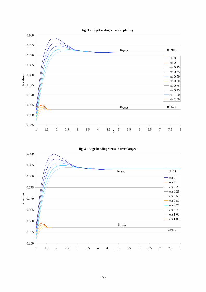
fig. 3 - Edge bending stress in plating

0.055

0.060

0.065

0.070

0.075

0.080

0.085

0.090

0.095

0.100

1 1.5 2 2.5 3 3.5 4 4.5 5 5.5 6 6.5 7 7.5 8ρρρρ

k va

lues

eta 0

eta 0

eta 0.25

eta 0.25

eta 0.50

eta 0.50

eta 0.75

eta 0.75

eta 1.00

eta 1.00

kYpSUP 0.0916

0.0627 kXpSUP

fig. 4 - Edge bending stress in free flanges

0.050

0.055

0.060

0.065

0.070

0.075

0.080

0.085

0.090

1 1.5 2 2.5 3 3.5 4 4.5 5 5.5 6 6.5 7 7.5 8ρρρρ

k va

lues

eta 0

eta 0

eta 0.25

eta 0.25

eta 0.50

eta 0.50

eta 0.75

eta 0.75

eta 1.00

eta 1.00

kXfSUP

0.0833

0.0571

kYfSUP

153

fig. 5 - Bending stress in free flanges at center

-0.005

0.000

0.005

0.010

0.015

0.020

0.025

0.030

0.035

0.040

0.045

0.050

1 1.5 2 2.5 3 3.5 4 4.5 5 5.5 6 6.5 7 7.5 8ρρρρ

k va

lues

eta 0

eta 0

eta 0.25

eta 0.25

eta 0.50

eta 0.50

eta 0.75

eta 0.75

eta 1.00

eta 1.00

kYfCEN 0.0417

kXfCEN

4. CONVERGENCE OF THE METHOD In the following, the influence of the number of harmonics on k values is shown. Particularly, assuming ρ=5 and η=0.50, M=N has been varied from 5 up to 100, in order to obtain a number of harmonics comprised between 25 and 10000. If the number of harmonics is > 4900, i.e. M=N > 70, a good convergence in the assessment of k values, and then of the proposed curves, is obtained for practical purposes, as it can be appreciated from fig. 6, 7, 8.

fig . 6 - kW convergence

0.00259

0.00260

0.00261

0.00262

0.00263

0.00264

0.00265

0.00266

0 1000 2000 3000 4000 5000 6000 7000 8000 9000 10000M x N

k W

fig. 7 - kYpSUP convergence

0.082

0.083

0.084

0.085

0.086

0.087

0.088

0.089

0.090

0.091

0.092

0 1000 2000 3000 4000 5000 6000 7000 8000 9000 10000M x N

k YfS

UP

fig. 8 - kXpSUP convergence

0.020

0.025

0.030

0.035

0.040

0.045

0.050

0.055

0.060

0.065

0 1000 2000 3000 4000 5000 6000 7000 8000 9000 10000M x N

k XfS

UP

154

5. THE CASE OF DISCONTINUOUS LOADS The partial differential equation (1) has been written with reference to a distributed normal pressure load which is a continuous function in the plate ℵ . Let’s now suppose that ( )Ω2Lp∈ , so that the set of

discontinuity points has zero measure according to Lebesgue. Let’s define with ℵ⊆ℵ0

the point set where p is

continuous and with ℵ⊂ℵ1: ( ) 01 =ℵm the point set

where p is discontinuous. The two subsets

0ℵ and 1ℵ define a partition of ℵ :

∅=ℵ∩ℵℵ=ℵ∪ℵ

10

10 (50)

Rigorously, as (1) is valid point by point only where p is continuous, the functional (19) has to be extended only to the

0ℵ domain. But, as p is continuous almost

everywhere in ℵ , the functional P(w) can be extended to the entire ℵ domain. It is noticed that, as ( )Ω2Lw∈ ,

according to the Schwartz-Holder inequality, ( )Ω1Lpw∈ , e.g. [4].

Moreover, as an integral extended to a set of zero measure is equal to zero according to Lebesgue, the following equalities hold:

ℵℵ∪ℵℵΠ=Π=Π )()()(

100www (51)

Then, it is possible to apply the equation (1) not only when the load function is continuous in ℵ, but also when it is continuous almost everywhere in ℵ , in both cases extending the functional (19) to the entire domain according to the identity (51). The extension to load functions continuous almost everywhere according to Lebesgue is particularly useful when it is necessary to schematize the wheeled loads. In this case, in fact, the effective load distribution can be modelled as an equivalent pressure, transversally constant but longitudinally discontinuous: ( ) [ ] [ ]1,0;,,. ∈∀∈∀= ηβαξηξ iiieq pp (52)

6. THE EQUIVALENT PRESSURE FOR WHEELED LOAS For primary supporting members subjected to wheeled loads, yielding checks have to be carried out considering a maximum pressure load, equivalent to the maximum vertical, static and dynamic, applied forces; the static part can be evaluated with the following relation, suggested by R.I.NA., 2005:

gs

XX

ls

Qnp AV

stateq

+−= 21

.. 3 (53)

in which it is assumed: • nV = maximum number of vehicles located on the primary supporting member; • QA = maximum axle load in t; • X1 = minimum distance, in m, between two consecutive axles; • X2 = minimum distance, in m, between the axles of two consecutive vehicles; • l = span, in m, of the primary supporting members; • s = spacing, in m, of primary supporting members. The maximum total equivalent pressure is the sum of the static term and the dynamic one and can be expressed in kN/m2 as follows: ( ) ..max. 1 stateqZeq pap += (54)

where aZ is the ship vertical acceleration. The following figure shows the origin of the formula (53).

s s

X1 X2

fig. 9

The three wheels give the following contributions to eq. (53):

• gls

Qnp AV

stateq =0..

• gs

Xs

ls

Qnp AV

stateq

−= 11..

• gs

Xs

ls

Qnp AV

stateq

−= 22..

The equation (53) is valid only if an axle is located directly on a supporting member, but if this condition is not verified the previous relation can’t be directly applied. So, it is convenient to generalize the eq. (53) as follows:

s s

Qi Q1Q2

X2X1Xi

fig. 10

gs

XQ

ls

np i

n

iiA

Vstateq

A

−= ∑=

11

.. (55)

155

where nA is the number of axles between –s and s and Xi is the distance of the i-th axle load from the considered supporting member. From eq. (55), the actual equivalent pressure pi, including inertial force, is obtained similarly to eq. (54). In such a way it is possible to model the load distribution on the deck on the basis of axle loads and geometric characteristics of vehicles. As in this case the deck isn’t loaded by a uniform pressure load, but by a load function discontinuous at intervals, the integral at the second term of (25) has to be replaced as follows:

=∂

∂∫ ∫1

0

1

0,

42 ηξdpwdw

anm

( ) ( ) =−−= ∑ ∫ ∫=

T i

i

n

iieq dndmap

1

1

0

4max. 2cos12cos12

β

α

ηηπξξπκ

∑=

−−−=Tn

i

iiiiieq

m

msenmsenap

1

4max.

2

222

παπβπαβκ (56)

where nT is the number of intervals where p is continuous, coinciding with the number of transverses, peq.max is the maximum equivalent pressure given by (54) and κi is defined as follows:

[ ]max.max.

,

eq

ii

eq

ii p

p

p

p βακ == (57)

7. ANALYSIS OF SOME TYPICAL RO-RO DECK STRUCTURES In the following it has been investigated the influence of the longitudinal distribution of wheeled loads on girder and transverse stresses, in order to highlight the “plate effect” which re-distributes the load peaks on transverses, unlike the isolated beam scheme. Two decks are analyzed: the first one is relative to a fast ferry, the second one to a Ro-ro Panamax ship ( see Campanile et al., 2007 ). 7.1 ANALYSIS OF A RO-RO FAST FERRY DECK It has been carried out the evaluation of the stresses acting on the primary supporting members of a fast ferry used to carry vehicles; the ship main dimensions are: Lbp = 97.61 m; B = 17.10 m ; D = 10.40 m; ∆ = 1420t. All transverses and girders have a 320x10+150x15 T section, while longitudinals are 60x6 offset bulb plates, in high-strength steel with syield=355 N/mm2. The data assumed in the analysis are: • LX=80 m; • l=LY=16 m; • sX = 2 m; • sY = 2 m; • seX = 0.5 m; • t = 8 mm; • X1 = 3000 mm;

• X2 = 2200 mm; • QA = 1.2 t; • nV = 7; • aZ= 0.909g; • IeX = 29146 cm4; • IeY = 29067 cm4; • IpX = 5190 cm4; • IpY = 5359 cm4; • rXf = 28.47 cm; • rYf = 28.38 cm; • ρ = 5; • ηt = 0.18. In fig. 11 the deck scheme is shown.

LC

200

0

2000

T320x100+150x15

T3

20x

10

0+

15

0x1

5

fig. 11

From (53) the maximum static equivalent pressure is peq.stat. = 2575 N/m2 so that, considering the vertical acceleration, the maximum total pressure is peq.max = 4914 N/m2. The longitudinal distribution of the equivalent pressure pi and σYfSUP stresses are listed in tab. 4 where: • Transv. indicates the current transverse; • X’ is the distance in mm of the first axle respect to the

current transverse in the interval [αi , βi ]; • X’’ is the distance in mm of the second axle (if

present) respect to the current transverse in the interval [αi , βi ];

• κi is the ratio between the pressure on the i-th transverse and the maximum one;

• αi indicates the aft limit, respect to the origin, of the i-th interval where p=pi is continuous;

• βi indicates the fore limit, respect to the origin, of the i-th interval;

• nA indicates the number of axles in the interval [αi , βi ];

• kYf–Orth. is the factor, determined by the orthotropic plate theory, to be inserted in (45.2) to determine the stress in the free flange of the i-th transverse with reference to p=peq.;

• kYf–FEM is the factor obtained by the FEM analysis of the corresponding structure.

156

Trans. X'

mm X'' mm κκκκi

ααααi

m ββββi

m nA

kYf Orth.

kYf FEM

1 1400 1600 0.50 1 3 2 0.0089 0.0109

2 400 1800 0.90 3 5 2 0.0269 0.0308

3 200 --- 0.90 5 7 1 0.0421 0.0476

4 800 --- 0.60 7 9 1 0.0525 0.0584

5 1200 1000 0.90 9 11 2 0.0592 0.0660

6 1000 --- 0.50 11 13 1 0.0636 0.0699

7 0 --- 1.00 13 15 1 0.0663 0.0730

8 200 --- 0.90 15 17 1 0.0655 0.0733

9 1800 1200 0.50 17 19 2 0.0645 0.0716

10 800 1400 0.90 19 21 2 0.0643 0.0717

11 600 --- 0.70 21 23 1 0.0644 0.0711

12 400 --- 0.80 23 25 1 0.0642 0.0710

13 1600 600 0.90 25 27 2 0.0632 0.0707

14 1400 1600 0.50 27 29 2 0.0631 0.0698

15 400 1800 0.90 29 31 2 0.0638 0.0707

16 200 --- 0.90 31 33 1 0.0637 0.0709

17 800 --- 0.60 33 35 1 0.0632 0.0699

18 1200 1000 0.90 35 37 2 0.0629 0.0702

19 1000 --- 0.50 37 39 1 0.0636 0.0698

20 0 --- 1.00 39 41 1 0.0648 0.0757

21 200 --- 0.90 41 43 1 0.0636 0.0711

22 1800 1200 0.50 43 45 2 0.0629 0.0696

23 800 1400 0.90 45 47 2 0.0632 0.0703

24 600 --- 0.70 47 49 1 0.0637 0.0691

25 400 --- 0.80 49 51 1 0.0638 0.0703

26 1600 600 0.90 51 53 2 0.0631 0.0706

27 1400 1600 0.50 53 55 2 0.0632 0.0699

28 400 1800 0.90 55 57 2 0.0642 0.0713

29 200 --- 0.90 57 59 1 0.0644 0.0708

30 800 --- 0.60 59 61 1 0.0643 0.0708

31 1200 1000 0.90 61 63 2 0.0645 0.0719

32 1000 --- 0.50 63 65 1 0.0655 0.0714

33 0 --- 1.00 65 67 1 0.0663 0.0725

34 200 --- 0.90 67 69 1 0.0636 0.0702

35 1800 1200 0.50 69 71 2 0.0592 0.0642

36 800 1400 0.90 71 73 2 0.0525 0.0570

37 600 --- 0.70 73 75 1 0.0421 0.0449

38 400 --- 0.80 75 77 1 0.0269 0.0282

39 1600 --- 0.20 77 79 1 0.0089 0.0094

tab. 4

The following diagrams show the equivalent pressure and the σYf stress longitudinal distribution.

Peq. longitudinal distribution

0

0.1

0.2

0.3

0.4

0.5

0.6

0.7

0.8

0.9

1

xxxx

κκ κκ i

fig. 12

kYf longitudinal distribution

0

0.1

0.2

0.3

0.4

0.5

0.6

0.7

0.8

0.9

1

xxxx

k 1

fig. 13

where:

.max

1−

=Yf

Yf

k

kk (58)

This analysis shows that there is a significant re-distribution of σYf stresses that can’t be evaluated by the isolated beam model. This effect unload the most loaded transverses and load the least loaded ones. The maximum stresses on girders and transverses are: • σXf = 100 N/mm2 • σYf = 163 N/mm2 It is noticed that by a coarse mesh FEM analysis the following maximum stresses have been obtained: • σXf-FEM= 115 N/mm2 • σYf-FEM= 175 N/mm2 If the deck were loaded by the uniform pressure p = 4914 N/m2, equal to the maximum equivalent pressure, from fig. 4 it is obtained that the maximum stresses on girders and transverses would be: • kXf-unif.= 0.0571→ σXf-unif.= 141 N/mm2 • kYf-unif.= 0.0833→ σYf-unif.= 205 N/mm2 Correspondingly by a coarse mesh FEM analysis, the following stresses have been obtained:

157

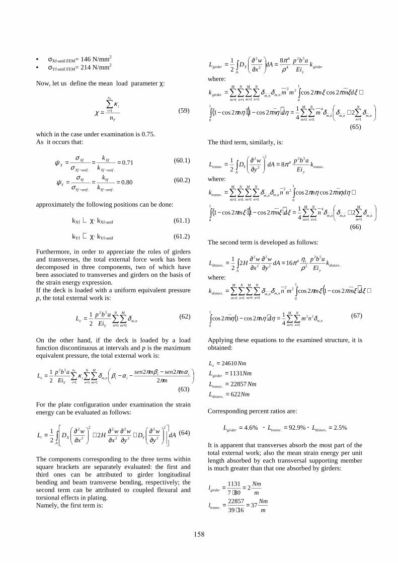
• σXf-unif.FEM= 146 N/mm2 • σYf-unif.FEM= 214 N/mm2 Now, let us define the mean load parameter χ:

T

n

ii

n

T

∑== 1

κχ (59)

which in the case under examination is 0.75. As it occurs that:

71.0..

===−− unifXf

Xf

unifXf

XfX k

k

σσ

ψ (60.1)

80.0..

===−− unifYf

Yf

unifYf

YfY k

k

σσ

ψ (60.2)

approximately the following positions can be done: kXf ≅ χ· kXf-unif (61.1)

kYf ≅ χ· kYf-unif (61.2)

Furthermore, in order to appreciate the roles of girders and transverses, the total external force work has been decomposed in three components, two of which have been associated to transverses and girders on the basis of the strain energy expression. If the deck is loaded with a uniform equivalent pressure p, the total external work is:

∑∑= =

=N

n

M

mnm

Ye Ei

abpL

1 1,

52

2

1 δ (62)

On the other hand, if the deck is loaded by a load function discontinuous at intervals and p is the maximum equivalent pressure, the total external work is:

∑∑∑= ==

−−−=N

n

M

m

iiiinm

n

ii

Ye m

msenmsen

Ei

abpL

T

1 1,

1

52

2

22

2

1

παπβπαβδκ

(63) For the plate configuration under examination the strain energy can be evaluated as follows:

dAy

wD

y

w

x

wH

x

wDL

A

YXi ∫

∂∂+

∂∂

∂∂+

∂∂=

2

2

2

2

2

2

22

2

2

22

1 (64)

The components corresponding to the three terms within square brackets are separately evaluated: the first and third ones can be attributed to girder longitudinal bending and beam transverse bending, respectively; the second term can be attributed to coupled flexural and torsional effects in plating. Namely, the first term is:

girderyA

Xgirder kEi

abpdA

x

wDL

52

4

4

2

2 8

2

1

ρπ=

∂∂= ∫

where:

⋅= ∫∑∑∑∑= = = =

ξξπξπδδ dmmmmk nm

M

m

N

n

M

m

N

nnmgirder 2cos2cos

1

0

22

,1 1 1 1

,

( )( )

+=−− ∑∑∑∫== =

N

nnmnmnm

M

m

N

n

mdnn1

,,,1 1

41

0

241

2cos12cos1 δδδηηπηπ

(65) The third term, similarly, is:

.

524

2

2

2

82

1transv

yA

Ytransv kEi

abpdA

y

wDL π=

∂∂= ∫

where:

⋅= ∫∑∑∑∑= = = =

ηηπηπδδ dnnnnk nm

M

m

N

n

M

m

N

nnmtransv 2cos2cos

1

0

22

,1 1 1 1

,.

( )( )

+=−− ∑∑∑∫== =

M

mnmnmnm

M

m

N

n

ndmm1

,,,1 1

41

0

241

2cos12cos1 δδδξξπξπ

(66) The second term is developed as follows:

.

52

24

2

2

2

2

. 16221

distorsy

t

A

distors kEi

abpdA

y

w

x

wHL

ρηπ=

∂∂

∂∂= ∫

where:

( ) ⋅−= ∫∑∑∑∑= = = =

ξξπξπδδ dmmmnk nm

M

m

N

n

M

m

N

nnmdistors 2cos12cos

1

0

22

,1 1 1 1

,.

( ) ∑∑∫= =

=−M

mnm

N

n

nmdnn1

,2

1

21

0 4

12cos12cos δηηπηπ (67)

Applying these equations to the examined structure, it is obtained:

NmLe 24610=

NmLgirder 1131=

NmLtransv 22857. =

NmLdistors 622. =

Corresponding percent ratios are:

%6.4=girderL - %9.92. =transvL - %5.2. =distorsL

It is apparent that transverses absorb the most part of the total external work; also the mean strain energy per unit length absorbed by each transversal supporting member is much greater than that one absorbed by girders:

m

Nmlgirder 2

807

1131=⋅

=

m

Nmltransv 37

1639

22857. =

⋅=

158

7.2 ANALYSIS OF A RO-RO PANAMAX DECK It has been carried out the evaluation of the highest stresses acting on the primary supporting members of a Ro-ro PANAMAX ship used to carry heavy vehicles; the ship main dimensions are: Lbp = 195.00 m; B =32.25 m; D = 25.92 m; ∆ = 44200 t. Transverses and girders, have, respectively, 970x11+320x30 and 970x12+280x30 T sections, while longitudinals are 240x10 offset bulb plates, in high-strength steel with syield = 355 N/mm2. The data assumed in the analysis are: • LX=160 m; • l=LY=24 m; • sX = 4 m; • sY = 2.463 m; • seX = 0.667 m; • t = 14 mm; • aZ= 0.411g; • nV = 8 ; • IeX = 967698 cm4; • IeY = 911559 cm4; • IpX= 178784 cm4; • IpY= 244515 cm4; • rXf = 83.66 cm; • rYf = 75.30 cm; • ρ = 7.41; • ηt = 0.22. The deck scheme is shown in fig. 14.

CL

T970x12+280x30

T9

70x

11

+3

20x3

04000

246

3

fig. 14

The reference vehicle has the main dimensions and the static axles loads shown in fig. 15.

15005285136016002545 3645

8 t 16 t 16 t 16 t 8 t

fig. 15

The maximum total pressure is peq.max = 48647 N/m2. The longitudinal distribution of the equivalent pressure is shown in tab.5.

Trans. QA1

t QA2 ( t )

QA3 ( t )

X1 (mm)

X2 (mm)

X3 (mm)

κκκκi

1 11.29 0 0 1997 0 0 0.06

2 11.29 22.58 0 466 1133 0 0.58

3 22.58 22.58 0 1329 30 0 0.89

4 22.58 0 0 2432 0 0 0.01

5 22.58 0 0 389 0 0 0.52

6 22.58 11.29 0 2073 1571 0 0.21

7 11.29 0 0 891 0 0 0.20

8 0 0 0 0 0 0 0.00

9 11.29 22.58 0 25 1625 0 0.51

10 22.58 22.58 0 837 522 0 0.89

11 22.58 0 0 1940 0 0 0.13

12 22.58 0 0 881 0 0 0.40

13 22.58 11.29 0 1581 2063 0 0.27

14 11.29 0 0 400 0 0 0.26

15 0 0 0 0 0 0 0.00

16 11.29 22.58 0 516 2116 0 0.33

17 11.29 22.58 22.58 1946 346 1013 0.96

18 22.58 0 0 1449 0 0 0.25

19 22.58 0 0 1372 0 0 0.27

20 22.58 0 0 1090 0 0 0.34

21 11.29 0 0 91 0 0 0.30

22 11.29 0 0 2371 0 0 0.01

23 11.29 0 0 1008 0 0 0.18

24 11.29 22.58 22.58 1454 145 1505 0.95

25 22.58 22.58 0 2317 957 0 0.41

26 22.58 0 0 1864 0 0 0.15

27 22.58 0 0 599 0 0 0.47

28 11.29 0 0 583 0 0 0.24

29 11.29 0 0 1880 0 0 0.07

30 11.29 0 0 1500 0 0 0.12

31 11.29 22.58 22.58 963 636 1997 0.76

32 22.58 22.58 0 1826 466 0 0.66

33 22.58 0 0 2356 0 0 0.03

34 22.58 0 0 107 0 0 0.59

35 11.29 0 0 1074 0 0 0.17

36 11.29 0 0 1388 0 0 0.13

37 11.29 0 0 1991 0 0 0.06

38 11.29 22.58 0 472 1128 0 0.58

159

39 22.58 22.58 0 1335 25 0 0.89

40 22.58 0 0 2438 0 0 0.01

41 22.58 0 0 384 0 0 0.52

42 22.58 11.29 0 2078 1566 0 0.21

43 11.29 0 0 897 0 0 0.20

44 0 0 0 0 0 0 0.00

45 11.29 22.58 0 20 1620 0 0.52

46 11.29 22.58 22.58 2443 843 517 0.89

47 22.58 0 0 1946 0 0 0.13

48 22.58 0 0 876 0 0 0.40

49 22.58 11.29 0 1587 2058 0 0.27

50 11.29 0 0 405 0 0 0.26

51 0 0 0 0 0 0 0.00

52 11.29 22.58 0 511 2111 0 0.33

53 11.29 22.58 22.58 1952 352 1008 0.96

54 22.58 0 0 1455 0 0 0.25

55 22.58 0 0 1367 0 0 0.27

56 22.58 0 0 1096 0 0 0.34

57 11.29 0 0 86 0 0 0.30

58 11.29 0 0 2377 0 0 0.01

59 11.29 0 0 1003 0 0 0.18

60 11.29 22.58 22.58 1460 140 1500 0.95

61 22.58 22.58 0 2323 963 0 0.41

62 22.58 0 0 1859 0 0 0.15

63 22.58 0 0 604 0 0 0.46

64 11.29 0 0 578 0 0 0.24

tab. 5

The following diagrams show the equivalent pressure and kYf longitudinal distribution.

Peq. longitudinal distribution

0.0

0.1

0.2

0.3

0.4

0.5

0.6

0.7

0.8

0.9

1.0

xxxx

κκ κκ i

fig. 16

kYf longitudinal distribution

0

0.1

0.2

0.3

0.4

0.5

0.6

0.7

0.8

0.9

1

xxxx

k 1

fig. 17

The maximum stresses on girders and transverses are: • σXf = 154 N/mm2 • σYf = 176 N/mm2 If the deck were loaded by the uniform pressure p = peq.max = 48647 N/m2, the maximum stresses on girders and transverses would be: • kXf-SUP-unif. = 0.0571 → σXf-unif. = 446 N/mm2 • kYf-SUP-unif. = 0.0833 → σYf-unif. = 475 N/mm2 so obtaining:

35.0k

k

.unifXf

Xf

.unifXf

XfX ===

−−σσψ (68.1)

37.0k

k

.unifYf

Yf

.unifYf

YfY ===

−−σσψ (68.2)

As in this case χ = 0.35 -see equation (59)-, approximately the positions (61.1) and (61.2) can be done, too. Concerning the strain energy components it is obtained:

NmLe 306225=

NmLgirder 18624=

NmLtransv 280462. =

NmLdistors 7139. =

Corresponding percent values are:

%0.6=girderL - %6.91. =transvL - %4.2. =distorsL

The mean strain energies per unit length absorbed by each transverse and each girder are:

m

Nml girder 23

1605

18624=⋅

=

m

Nml transv 183

2464

280462. =

⋅=

160

8. PRELIMINARY DIMENSIONING OF RO-RO DECK PRIMARY SUPPORTING MEMBERS Previous analyses have shown that the effective wheeled load distribution, expressed by means of the mean load parameter χ, has great influence on the loading of girders and transverses. Particularly, it has been observed that transverses absorb the great part of the load, while girders contribute to a re-distribution of stresses, unloading the most loaded transverses and loading the least loaded ones. In a previous work, see [6], a procedure for dimensioning of girders and transverses on the basis of the orthotropic plate theory has been proposed, considering a uniform pressure on deck and so neglecting the effective load longitudinal distribution. From the numerical results of sections 7.1 and 7.2 it seems appropriate to assume for the pressure the mean equivalent pressure load χpeq.max. Moreover, as for garage decks the aspect ratio r is much greater than 1, it is possible to assume kYf-SUP = 0.0833 and kX f-SUP = 0.0571. Indicating with σall tr. and σall long. the allowable stresses for transverses and girders respectively, and with peq.max the maximum pressure transmitted by wheels according to equation (54) it’s possible to calculate the section modulus for transverses by the following relation:

..

2max.

.

0833.0

trall

YYeqeYMIN

sLpW

σχ

⋅⋅⋅≥ (69)

where peq.max is in N/m2, LY and sY in m, σall.tr. in N/mm2 and WeYMIN. in cm3.The modulus is inclusive of plating effective breadth beY. The condition valid for girders is:

Xf

longalleY

YXYeqeXf r

I

ssLpW

2..

42max.2 0033.0

σχ

⋅⋅⋅⋅⋅

≥ (70)

where peq.max is in N/m2, LY, sY and sX in m, IeY in cm4, rXf in cm, σall.long. in N/mm2 and WeXf in cm3. 9. CONCLUSIONS In this work the orthotropic rectangular plate bending equation with all edges clamped has been solved adopting the Rayleigh-Ritz method. Numerical calculations have been systematically performed in case of uniform pressure, varying two non-dimensional parameters, namely the virtual side ratio and the torsional coefficient. Response non-dimensional parameters, in terms of maximum deflection and maximum stresses, are given in a series of charts for their easy application. Some comparisons with well known published data and FEM analyses give a validation to the method. The method has been applied to ro-ro garage decks, taking into account in this case a load variable along the

deck length, according to the geometrical and mass characteristics of the reference vehicle. Two typical ro-ro ships have been examined. It has been highlighted that transverse beams absorb the most part of the external work done by the pressure load, as it could be expected. Besides, it has been found that there is an appreciable re-distribution of the load, so that almost the same maximum stresses are obtained considering simply the mean pressure acting uniformly on the deck; then those stresses can be evaluated directly by the orthotropic plate charts. From that, the suggestion for a simple procedure for the preliminary dimensioning of ro-ro deck primary supporting members is given. 10. REFERENCES 1. SCHADE H.A., ‘Design Curves for Cross-Stiffened Plating under Uniform Bending Load’, Trans. SNAME, 49, 1941. 2. TIMOSHENKO S., WOINOWSKY-KRIEGER S., ‘Theory of Plates and Shells’, Mc-Graw-Hill Book Company, 1959. 3. YOUNG D., ‘Analysis of Clamped Rectangular Plates’, Journal of Applied Mechanics, Volume 7, No.4, December 1940. 4. FIORENZA R., ‘Appunti delle lezioni di Analisi Funzionale’, Gli Strumenti di Coinor, 2005. 5. RINA, ‘Rules for the Classification of Ships’, 2005. 6. CAMPANILE A., MANDARINO M., PISCOPO V., “Considerations on dimensioning of garage decks”, ICMRT 2007.

161