Application of the Explicit Asymptotic Method to Nuclear Burning
47
University of Tennessee, Knoxville Trace: Tennessee Research and Creative Exchange Masters eses Graduate School 8-2009 Application of the Explicit Asymptotic Method to Nuclear Burning in Type Ia Supernova Christopher Ryan Smith University of Tennessee - Knoxville, [email protected] is esis is brought to you for free and open access by the Graduate School at Trace: Tennessee Research and Creative Exchange. It has been accepted for inclusion in Masters eses by an authorized administrator of Trace: Tennessee Research and Creative Exchange. For more information, please contact [email protected]. Recommended Citation Smith, Christopher Ryan, "Application of the Explicit Asymptotic Method to Nuclear Burning in Type Ia Supernova. " Master's esis, University of Tennessee, 2009. hps://trace.tennessee.edu/utk_gradthes/546
Transcript of Application of the Explicit Asymptotic Method to Nuclear Burning

University of Tennessee, KnoxvilleTrace: Tennessee Research and CreativeExchange
Masters Theses Graduate School
8-2009
Application of the Explicit Asymptotic Method toNuclear Burning in Type Ia SupernovaChristopher Ryan SmithUniversity of Tennessee - Knoxville, [email protected]
This Thesis is brought to you for free and open access by the Graduate School at Trace: Tennessee Research and Creative Exchange. It has beenaccepted for inclusion in Masters Theses by an authorized administrator of Trace: Tennessee Research and Creative Exchange. For more information,please contact [email protected].
Recommended CitationSmith, Christopher Ryan, "Application of the Explicit Asymptotic Method to Nuclear Burning in Type Ia Supernova. " Master's Thesis,University of Tennessee, 2009.https://trace.tennessee.edu/utk_gradthes/546

To the Graduate Council:
I am submitting herewith a thesis written by Christopher Ryan Smith entitled "Application of the ExplicitAsymptotic Method to Nuclear Burning in Type Ia Supernova." I have examined the final electronic copyof this thesis for form and content and recommend that it be accepted in partial fulfillment of therequirements for the degree of Master of Science, with a major in Physics.
Michael Guidry, Major Professor
We have read this thesis and recommend its acceptance:
ARRAY(0x7f70290bc320)
Accepted for the Council:Dixie L. Thompson
Vice Provost and Dean of the Graduate School
(Original signatures are on file with official student records.)
To the Graduate Council:
I am submitting herewith a dissertation written by Christopher Ryan Smith entitled Application of the Ex-
plicit Asymptotic Method to Nuclear Burning in Type Ia Supernova. I have examined the final electronic
copy of this dissertation for form and content and recommendthat it be accepted in partial fulfillment of the
requirements for the degree of Master of Science, with a major in Physics.
Michael Guidry, Major Professor
We have read this thesisand recommend its acceptance:
Otis Messer
William Raphael Hix
Accepted for the Council:
Carolyn R.HodgesVice Provost andDean of the Graduate School
Application of the Explicit Asymptotic Method to
Nuclear Burning in Type Ia Supernova
A Thesis
Presented for the
Master of Science
Degree
The University of Tennessee, Knoxville
Christopher Ryan Smith
August 2009

Copyright © 2009 by Christopher Smith.
All rights reserved.
ii
Acknowledgments
I would first like to thank my advisor Dr. Michael Guidry for accepting me as a Master’s student. Without
his knowledge and insight, this project could not have happened. For his frequent assistance dealing with
the intricacies of FLASH, I must thank Dr. Otis Messer. He wasable to provide insight into the workings
of the code that allowed problems to be overcome in hours or days instead of weeks. Dr. Viktor Chupryna,
whose work laid the foundation for my own, was of much help in my understanding of how FLASH and our
burner were organized. Elisha Feger, with whom I shared an office for the later part of my work, was always
willing to lend his knowledge of FLASH and coding in general.I must also thank Rachel Ainsworth who
was kind enough to lend her time in assisting me with the visualization of my data. Finally, I would like to
thank the entire Department of Physics and Astronomy, of which I have been a part for the last seven years,
for all the help and support over during my time here.
iii
Abstract
Modern problems in astrophysics tend to require large, complex computational frameworks to solve many
aspects of the system simultaneusly. Calculation of the energy production through nuclear reactions is
typically one of those aspects. The use of standard nuclear burning algorithms will take up the majority of
the computational time with all but the smallest of networks. The explicit asymptotic method has shown
promise in computing large networks faster than existing methods in various environments while retaining
accuracy. The purpose of this thesis is to show that this method can be successfully used to solve complex
systems using a network of realistic size in a reasonable amount of time, and to investigate some problems
in the flame propagation for a Type Ia, which have never been investigated with a realistic network.
iv

Contents
1 Introduction 1
2 Supernova Type Ia 2
2.1 Classification . . . . . . . . . . . . . . . . . . . . . . . . . . . . . . . . . . .. . . . . . . 2
2.2 Evolution . . . . . . . . . . . . . . . . . . . . . . . . . . . . . . . . . . . . . . .. . . . . 4
2.2.1 Progenitors . . . . . . . . . . . . . . . . . . . . . . . . . . . . . . . . . . .. . . . 4
2.2.2 Pre-Ignition . . . . . . . . . . . . . . . . . . . . . . . . . . . . . . . . . .. . . . . 5
2.2.3 Explosion . . . . . . . . . . . . . . . . . . . . . . . . . . . . . . . . . . . . .. . . 5
2.3 Type Ia and Cosmology . . . . . . . . . . . . . . . . . . . . . . . . . . . . . .. . . . . . . 7
3 Computational Modeling of Type Ia Supernova 8
3.1 Computational Difficulties . . . . . . . . . . . . . . . . . . . . . . . .. . . . . . . . . . . 8
3.2 FLASH Code . . . . . . . . . . . . . . . . . . . . . . . . . . . . . . . . . . . . . . .. . . 9
3.2.1 Hydrodynamics . . . . . . . . . . . . . . . . . . . . . . . . . . . . . . . . .. . . . 11
3.3 Explicit Asymptotic Method . . . . . . . . . . . . . . . . . . . . . . . .. . . . . . . . . . 11
3.3.1 Recent Progress . . . . . . . . . . . . . . . . . . . . . . . . . . . . . . . .. . . . . 13
4 Results 17
4.1 Results Using an Explicit 13 Isotope Alpha Network . . . . .. . . . . . . . . . . . . . . . 18
4.1.1 Hard Barriers in FLASH . . . . . . . . . . . . . . . . . . . . . . . . . . .. . . . . 18
4.1.2 Ash hemispheres . . . . . . . . . . . . . . . . . . . . . . . . . . . . . . . .. . . . 18
4.2 Results using 150-Isotope Network . . . . . . . . . . . . . . . . . .. . . . . . . . . . . . . 26
v

5 Conclusions 29
5.1 Current Progress . . . . . . . . . . . . . . . . . . . . . . . . . . . . . . . . .. . . . . . . 29
5.2 Future Work . . . . . . . . . . . . . . . . . . . . . . . . . . . . . . . . . . . . . .. . . . . 30
Vita 35
vi
List of Tables
4.1 Initial Conditions, Approx13 . . . . . . . . . . . . . . . . . . . . . .. . . . . . . . . . . . 18
4.2 Initial Conditions, 150 Isotope Network . . . . . . . . . . . . .. . . . . . . . . . . . . . . 26
vii
List of Figures
2.1 The current classification of supernovae . . . . . . . . . . . . .. . . . . . . . . . . . . . . 3
2.2 Typical light curves from each sub-type of supernova. [3] . . . . . . . . . . . . . . . . . . . 4
2.3 Development of a bubble. [47] . . . . . . . . . . . . . . . . . . . . . . .. . . . . . . . . . 6
2.4 The Gravitationally Confined Detonation Mechanism [50]. . . . . . . . . . . . . . . . . . 6
3.1 Difference in the scales that must be considered in a TypeIa. [45] . . . . . . . . . . . . . . 9
3.2 Numerical solutions to Equation 3.1 using different timesteps. [46] . . . . . . . . . . . . . 10
3.3 Fluxes and the asymptotic approximation. Three isotopes are shown from an alpha network
run under constant conditions T= 3×10⁹K andρ = 1×10⁷gcm−3 [49] . . . . . . . . . . . 12
3.4 Network timestepsdt and maximum explicit timestep 1/(maxrate) for the calculation illus-
trated in Fig. 3.3 [49] . . . . . . . . . . . . . . . . . . . . . . . . . . . . . . . .. . . . . . 13
3.5 Integration timesteps in the CNO cycle for the explicit asymptotic integrator. The upper plot
shows the ratio of the actual timestep to the maximum expected to be stable for a normal
explicit method, estimated as 1/(max rate). [49] . . . . . . . . .. . . . . . . . . . . . . . . 14
3.6 Results: 150-Isotope Network as of December, 2008. [45]. . . . . . . . . . . . . . . . . . 15
3.7 Results: 150-Isotope Network as of July, 2009. . . . . . . . .. . . . . . . . . . . . . . . . 16
4.1 12C mass fraction at various times on a log scale from [48]. . . . .. . . . . . . . . . . . . . 19
4.2 Initial temperature distribution using a logarithmic scale for the case with barriers. . . . . . 20
4.3 12C mass fraction at various times on a log scale. . . . . . . . . . . . .. . . . . . . . . . . 21
4.4 12C mass fraction at various times on a log scale. . . . . . . . . . . . .. . . . . . . . . . . 22
4.5 12C mass fraction at various times on a log scale. . . . . . . . . . . . .. . . . . . . . . . . 23
viii

4.6 Velocity in the x direction in units of cm s−1 . . . . . . . . . . . . . . . . . . . . . . . . . 24
4.7 Initial temperature distribution using a logarithmic scale for the case with hemispheres of ash. 24
4.8 12C mass fraction at various times on a log scale. . . . . . . . . . . . .. . . . . . . . . . . 25
4.9 Temperature plot from single block EOS test using the 150-isotope network. The left half
is fuel and the right ash. . . . . . . . . . . . . . . . . . . . . . . . . . . . . . .. . . . . . . 28
ix

Chapter 1
Introduction
Supernovae are some of the most energetic objects in the universe. A typical one will emit as much light as
an entire galaxy during its short lifetime. They are also theprimary source for elements up to the iron group.
In addition, modern cosmology relies on Type Ia supernovae in particular for the accurate measurements of
distance that are so important in that field. Therefore, it isonly natural that they would be of much interest
to the field of astrophysics. However, they are also some of the most complex systems that exist and require
knowledge from most branches of physics and advanced computational methods in order to study them.
Because of their complexity, it has only been recently that computational power and numerical algo-
rithms have developed sufficiently to allow the study of manyof the details of the supernova problem. The
research discussed in this thesis has been focused on the implementation of a new method of studying the
nuclear burning that takes places within all stars. This hasbecome particularly important in the study of
Type Ia supernova which are believed to occur when a white dwarf is consumed in a thermonuclear run-
away. Historically, the problem was investigated in a very limited form using at most the first 13 elements
in the alpha chain. Often even smaller networks, or in some cases no network at all, were used due to the
complexity of the reactions involved. This study aims to demonstrate a method for calculating the nuclear
reactions that allows for the use of a realistically sized network, and show that the results agree with those
obtained using more conventional methods.
1

Chapter 2
Supernova Type Ia
2.1 Classification
Supernovae are classified into two main types each with several subtypes based on the spectral properties
they display (Figure 2.1). This is done by careful measurement of the intensity and the spectra throughout
the evolution of the supernova. Type I supernovae all display weak hydrogen lines at early times, while the
spectra for a Type II is dominated by the Hα lines. Type I supernovae are divided into three sub-groups,
again based on their spectral properties at different times. Type Ib and Ic are characterized by a lack of Si
II at early times, a feature which is prominent in Type Ia. Types Ib and Ic are then differentiated by the
strength of the helium lines. Type Ib are rich in helium, while Type Ic supernovae are not.
In contrast to the Type I’s, Type II supernovae are classifiedby the shape of the light curve rather
than their spectra, specifically how the curve behaves afterthe maximum (Figure 2.2). Type IIL and IIP
supernovae have light curves that become linear or plateau,respectively, after the maximum intensity. The
third Type II, Type IIb, has a light curve that resembles Types Ib and Ic except for the lack of hydrogen.
As such, they are considered to be an intermediate between the other Type II’s and the Type I’s. There is a
fourth Type II that is not shown on the figure, Type IIn. These supernovae are characterised by the narrow
hydrogen lines that appear in their spectra.
All supernovae other than Type Ia are believed to be caused bya similar mechanism called a core
collapse. That is they occur when the core of a massive star (>8 M⊙) collapses in on itself and forms a
neutron star or black hole, with the primary difference between the types being the composition of their
2

HHe
HHe
(H)HeMantle
WDAccretion
He
Hydrogen inEarly Spectra?
YesNo
SN ISilicon Lines?
SN IIDetailed Lightcurve Shape?
YesNo
SN Ia
HeliumRich?
YesNo
SN Ic SN Ib SN IIb SN IIL SN IIP
Core CollapseType II lightcurve:
linear after maximum
Core CollapseType II lightcurve:
plateau after maximum
Core CollapseMost H removed before collapse
(bridge II to Ib, Ic)
ThermonuclearThermonuclear
runaway, accreting C/O white dwarf
Core CollapseH removed before
collapse
Core CollapseH and much of He removed before
collapse
Figure
2.1:Th
ecu
rrentclassificatio
no
fsup
ernovae
3
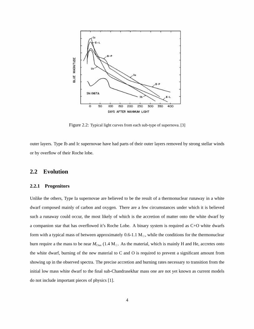
Figure 2.2:Typical light curves from each sub-type of supernova. [3]
outer layers. Type Ib and Ic supernovae have had parts of their outer layers removed by strong stellar winds
or by overflow of their Roche lobe.
2.2 Evolution
2.2.1 Progenitors
Unlike the others, Type Ia supernovae are believed to be the result of a thermonuclear runaway in a white
dwarf composed mainly of carbon and oxygen. There are a few circumstances under which it is believed
such a runaway could occur, the most likely of which is the accretion of matter onto the white dwarf by
a companion star that has overflowed it’s Roche Lobe. A binarysystem is required as C+O white dwarfs
form with a typical mass of between approximately 0.6-1.1 M⊙, while the conditions for the thermonuclear
burn require a the mass to be nearMChan (1.4 M⊙. As the material, which is mainly H and He, accretes onto
the white dwarf, burning of the new material to C and O is required to prevent a significant amount from
showing up in the observed spectra. The precise accretion and burning rates necessary to transition from the
initial low mass white dwarf to the final sub-Chandrasekhar mass one are not yet known as current models
do not include important pieces of physics [1].
4

2.2.2 Pre-Ignition
As the mass approaches the Chandrasekhar limit, the increased pressure will cause the carbon in the core
to begin to smolder. Since the matter in the white dwarf is degenerate, the energy release will not go into
expanding the star and will instead cause the temperature inthe core to increase. During the smoldering
phase, convection sets up in the white dwarf involving the majority of the star and leads to a near uniform
composition [15]. This lasts until the star reaches a temperatures of approximately 1×10⁹ K, at which point
the energy production by carbon burning exceeds the rate at which the convection can remove it [15]. This
is the start of the thermonuclear runaway.
2.2.3 Explosion
The specifics of how the explosion progresses are still underdebate, but the general mechanism seems to
be understood. After reaching the critical temperature, a point near the core will ignite and begin to burn
outward. This burning will raise the degeneracy of the matter slightly causing it to expand, after which
buoyancy will cause the newly formed bubble to rise and expand (Fig. 2.3). The burn front as represented
by the edge of the bubble continues to expand as it rises. The velocity of the burn tends to increase linearly
with its area. As seen in the figure, the surface of the bubble tends to get more convoluted over time as a
result of the development of instabilities such as Rayleigh-Taylor. So far, the burn has been in what is known
as a deflagration phase: the burn front has been moving at lessthan the speed of sound. From observations
of the relative amounts and energies of various isotopes, particularly 56Ni and 28Si, we know that at some
point during the explosion the burn has to transition to a detonation where the burn front moves faster than
the speed of sound in the material. There are various theories as to how this might happen, but this paper will
assume that it is by gravitationally confined detonation (GCD). In the GCD case, the bubble will continue
to expand until it eventually reaches the surface of the white dwarf. It will then break free, but the material
will lack the velocity needed to escape the stars gravity andas such will proceed to expand outward above
and around the surface in a wave. Eventually, the material will collide with itself at a point almost directly
opposite that at which it originally broke out (Fig. 2.4). This collision will drive the material into the surface
and spark the detonation that will consume the rest of the star [47].
5

Figure 2.3:Development of a bubble. [47]
Asymmetric
bubble
breakout
Gravity-confined
burn front
Gravity-confined
burn front
Supersonic collision
drives shock into
white dwarf
Detonation
wave
White
dwarf
Figure 2.4:The Gravitationally Confined Detonation Mechanism [50]
6
2.3 Type Ia and Cosmology
As observational techniques have improved over the years, the ability to accurately gauge the distance an
object is from Earth has become increasingly important. This is normally done by using what are called
standard candles, classes of objects that have well defined luminosities that show little deviation between
the members. Type Ia’s show too much variation to be considered standard candles, however all Type Ia’s
display remarkably similar shapes in their light curves, absolute magnitudes, and spectra. The differences
that are observed can be corrected for with a single parameter that describes the strength of the explosion [1].
They are therefore considered to be standardizable candles.
As measuring devices, the Type Ia supernova have served astronomers and cosmologists well, but there
is still a significant amount of uncertainty inherent in their distance calculations. This is, of course, partially
caused by imperfections in the observational data itself, but a significant amount of the uncertainty comes
from a lack of understanding about the mechanism behind the supernova. With a better understanding of
the explosion, the accuracy of Type Ia Supernova measurement should improve. This has become especially
important in the last few decades as evidence has accumulated which indicates that the expansion of the
universe is increasing. An accurate measurement of the rateof expansion is vital to understanding many
fundamental questions currently faced, such as the nature of dark energy.
7
Chapter 3
Computational Modeling of Type Ia
Supernova
3.1 Computational Difficulties
When modeling any astrophysical process, one of the most common difficulties that must be overcome is
range of physical scales that must be considered, and the Type Ia supernova is no different (Fig. 3.1). The
white dwarf itself is on the order of ten thousand kilometersin diameter while the flame itself is a centimeter
or less in thickness [19] [20]. Fully resolving these disparate scales is out of the realm of possibility for
modern computational resources, the size of a typical comutational cell is one kilometer, so simpler models
that approximate the correct results by statistical or other means must be employed. In addition to problems
of scale, there is also the issue of stiffness. A stiff problem is one in which the timestep (∆t) needed to
fully resolve the problem is limited by stability rather than accuracy considerations. An example of a stiff
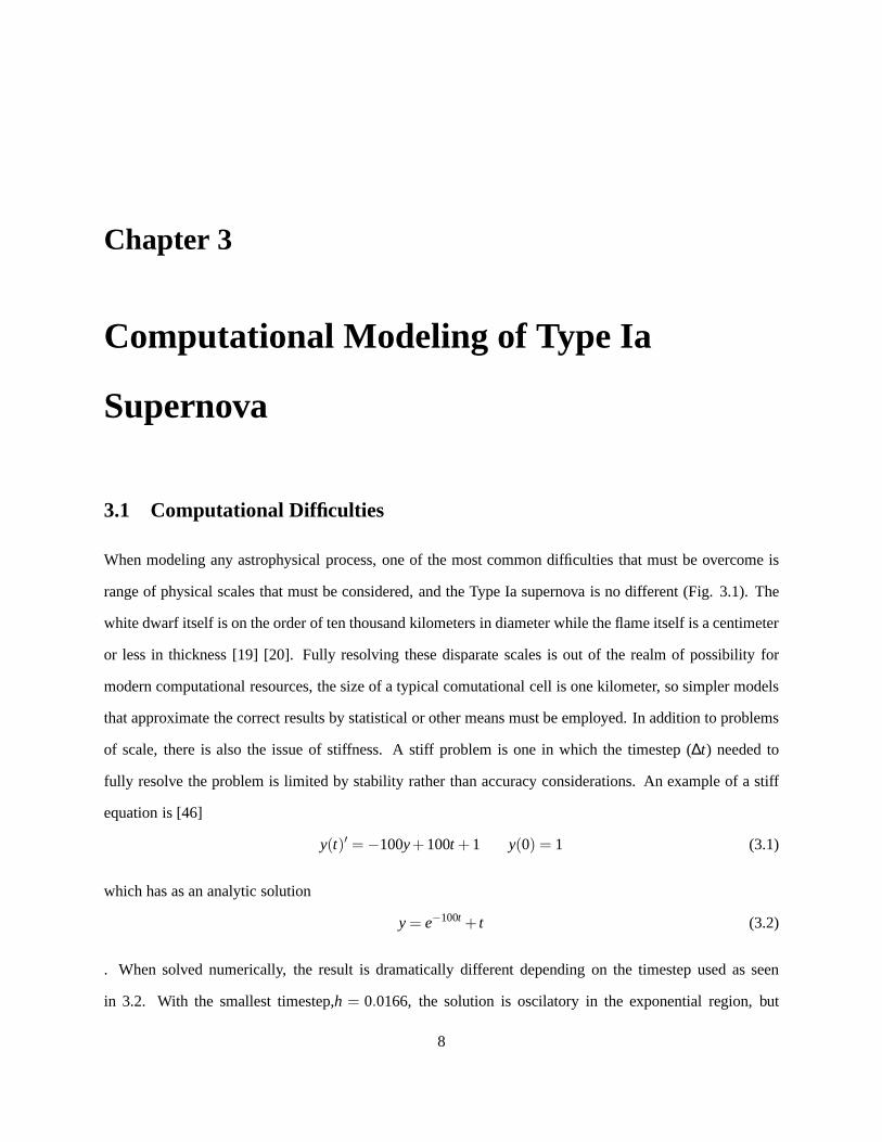
equation is [46]
y(t)′ = −100y+100t +1 y(0) = 1 (3.1)
which has as an analytic solution
y = e−100t + t (3.2)
. When solved numerically, the result is dramatically different depending on the timestep used as seen
in 3.2. With the smallest timestep,h = 0.0166, the solution is oscilatory in the exponential region,but
8

White Dwarf
~10,000 km
A typical
computational cell:
~1 km diameter
Characteristic
flame width:
0.001 - 10 cm
Figure 3.1:Difference in the scales that must be considered in a Type Ia.[45]
quickly approches the analytic solution after the functionbecoes linear. The intermediate timestep,h = 0.02,
oscilates about the solution throughout the entire extent.For the largest timestep,h = 0.03 the numerical
solution is completely unstable and eventually goes to infinity [46].
3.2 FLASH Code
The FLASH code, developed by the Center for Astrophysical Thermonuclear Flashes at the University of
Chicago, is a multi-dimensional hydrodynamics code using Adaptive Mesh Refinement (AMR) designed
to solve problems involving thermonuclear burning. It is written mainly in Fortran 90 using the Message-
Passing Interface (MPI) for parallelism and portability. FLASH is written in a modular form to allow for
quick swapping of physics solvers. The software package comes with many modules already included
which can be combined to solve a large selection of problems.The modular nature of the software allows
for the implementation of new physics without a substantialrewriting of the entirety of the code. FLASH
also utilizes a shared datastructure that all modules can access to store any variables that may be needed
by multiple parts of the code without the need to pass variables explicitly. Due to the modular nature, our
changes were able to be implemented through two modules: Composition and Burn (submodules of the
Equation of State and Source Terms respectively) [45].
9
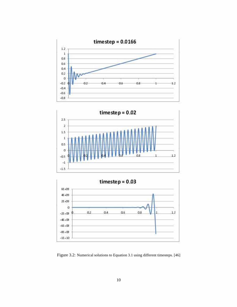
Figure 3.2:Numerical solutions to Equation 3.1 using different timesteps. [46]
10

3.2.1 Hydrodynamics
As mentioned earlier, the FLASH code allows for the linking of the multi-dimensional hydrodynamics with
the nuclear burning. On the hydrodynamics end, FLASH employs an AMR routine, which can increase the
resolution of the grid by, in 2D, creating 4 smaller blocks toreplace a larger one when a given condition is
met, such as a gradient becoming too steep, and decrease the resolution by merging the four blocks back
into one when the flux goes back below a threshold. This allowsFLASH to scale the current resolution
between a given maximum and minimum as needed as the problem progresses. This is highly desirable
in a supernova problem as in the majority of the star, FLASH would only need to be able to resolve the
hydrodynamics of the problem and the nuclear burning would only be resolved in the regions where burning
is taking place, leading to a substantial decrease in the computational resources required. Another necessary
component is the equation of state, which determines the thermodynamic properties of the fluids. In our
case, the Helmholtz equation of state was used [24]. This EOSuses an interpolated table to solve the
differential equations for an electron-positron plasma. This still yields correct results with other materials
since a simple multiplication of the result byYe, the number of electrons per baryon, will give the answer for
the desired fluid. The Helmholtz EOS is desirable primarily because it is valid for a degenerate gas, unlike
the other EOSs that are available in FLASH.
3.3 Explicit Asymptotic Method
The thermonuclear burning module used in this paper is an implementation of an explicit asymptotic method
[46]. The algorithm used in the Flux Limited Forward Differencing (FLFD) method was originally devel-
oped by M.W. Guidry [49] and added to the FLASH software by V. Chupryna [45]. It is an explicit stochastic
method for modeling systems with large numbers of particles. It uses Forward Euler differencing to solve
for the abundance at the next time given the current abundance, the number of test particles changing from
one isotope to another (the flux), and the the timestep. An additional restriction must be put on the values
of the fluxes to prevent the propagation of a negative population. To ensure that this does not occur, the
fluxes are constrained such thatFi j ≥ 0, whereFi j is the flux of particles from isotope i into isotope j. This
allows the algorithm to take much larger timesteps than it would normally as the slight negative populations
introduced by numerical errors are a major limiter on the size of the timestep in many explicit methods.
11

log flu
x
log time
-12
-15
-10
-5
0
5
10
-10 -8 -6 -4 -2 0 2 4 6 -12 -10 -8 -6 -4 -2 0 2 4 6 -12 -10 -8 -6 -4 -2 0 2 4 6
F+
F-
F
kdt4He
F
kdt
20Ne
F
kdt
28Si
F+
F+F
-
F-
Figure 3.3:Fluxes and the asymptotic approximation. Three isotopes are shown from analpha network run under constant conditions T= 3×10⁹K andρ = 1×10⁷gcm−3 [49]
The FLFD method works well as long as the fluxes are not in the asymptotic region. In this region
the incoming and outgoing fluxes are both very large, and the differences between them are many orders
of magnitude less than the fluxes themselves. Once the calculation enters the asymptotic region, a small
numerical error in the flux can lead to a large error in the actual rate, and therefore the timesteps tend to
crash. The rates for some isotopes can become asymptotic very early in the calculation, while some may
never, as shown in Fig 3.3. An explicit asymptotic method wasthen developed to deal with this situation as
detailed in [45]. The derivation discussed eventually yields the new equation for for the population
y(2)n ≃
F+n
kn−
1kn∆t
(
F+n
kn−
F+n−1
kn−1
)
(3.3)
ki≡
F−i
yi(3.4)
Whereyn is the abundance of isotope n,F− is the sum of the rates that deplete isotope n,F+ is the sum of
the rates that increase n, andF/eqF+ +F−. The method that is used in a given situation is decided for each
isotope as follows
1. If ki∆t<1, use the flux-limiting explicit algorithm.
2. Otherwise, update the population using the approximation given in Equation 3.3.
12

dt
1/(max rate)
log tim
e (
s)
log time (s)
-12
-12
-10
-8
-6
-4
-2
-9 -6 -3 0 3 6
Figure 3.4: Network timestepsdt and maximum explicit timestep 1/(maxrate) for thecalculation illustrated in Fig. 3.3 [49]
Through the use of the asymptotic approximation, we are ableto take increasing larger timesteps as
more and more of the rates become asymptotic. The speed increase over an explicit method limited by
the maximum rate is clearly shown in Fig. 3.4 for a simple integration of the CNO cycle. Also, it should
be noted that the region in which the timestep for the asymptotic method is greater than that for a normal
explicit method is also the region that takes most of the calculation time due to the plot being log/log in time.
An extreme example of this is given in figure 3.5 for the CNO cycle where a calculation that would take the
explicit asymptotic method one second would take a standardmethod longer than the ago of the universe.
3.3.1 Recent Progress
There have been several changes that have been incorporatedinto the FLASH code since the publication
of [45]. They are mainly corrections to the way the code had been implemented at the time, along with a
few slight improvements in performance, the most importantof which is the change to a realistic equation of
state which is better suited to the conditions encountered during a Type Ia simulation than the polytropic EOs
used in earlier tests. The changes lead to the calculation yielding qualitatively different results as can be seen
by comparing Fig. 3.6 and Fig. 3.7. Both calculations were made using an 150-isotope nuclear network and
only calculated a single computational zone. The initial conditions were a composition of 50/50 carbon and
oxygen with a temperature of T9=3K andρ = 1×10⁷ g cm−3. Most notably the oxygen burn occurs much
13

1020
1016
1012
108
104
Tim
este
p (
s)
1018
109
100
Ra
tio
106 109 1012 1015 1018 1021
Time (s)
dt
1/(max rate)
Figure 3.5:Integration timesteps in the CNO cycle for the explicit asymptotic integrator.The upper plot shows the ratio of the actual timestep to the maximum expected to be stablefor a normal explicit method, estimated as 1/(max rate). [49]
14
Figure 3.6:Results: 150-Isotope Network as of December, 2008. [45]
later than the carbon in the current results, rather than immediately following it. Also while the carbon flash
still occurs in a narrow region, it no longer resembles a delta function. While the speed has also increased by
a factor on the order of 100 since December (the original calculation took approximately 9hrs to run, while
the newer case ran in 35min, both on a single processor), there are still many improvements to be made to
the code in the way of optimization, both through improvements of the algorithm and standard numerical
optimization.
15

-7.96910 -6.77523 -5.58136 -4.38749 -3.19362 -1.99976
-14.0
-13.0
-12.0
-11.0
-10.0
-9.0
-8.0
-7.0
-6.0
-5.0
-4.0
-3.0
-2.0
-1.0
0.0
20:10:24 Jul 6, 2009|avalon|FLASHAsy
t=0.0s|SF=0.2|dX=1.0E-7|Ymin=0.0|Iso=150/150/150|sumX=0.9900|E/A=3.0714E-85|normX=false
Hydro=FLASH|Net=FLASH|Rates=all|InitY=FLASH
Log Time (seconds)
Log X (150 isotopes; legends 101 largest) Z=8 N=8
Z=14 N=14
Z=6 N=6
Z=16 N=16
Z=10 N=10
Z=12 N=12
Z=26 N=28
Z=18 N=18
Z=20 N=20
Z=28 N=28
Z=27 N=28
Z=28 N=30
Z=28 N=29
Z=26 N=27
Z=26 N=26
Z=2 N=2
Z=24 N=26
Z=19 N=20
Z=1 N=0
Z=17 N=18
Z=16 N=17
Z=25 N=26
Z=15 N=16
Z=14 N=16
Z=13 N=14
Z=18 N=20
Z=14 N=15
Z=16 N=18
Z=26 N=29
Z=27 N=29
Z=24 N=24
Z=18 N=19
Z=25 N=28
Z=27 N=30
Z=24 N=25
Z=20 N=21
Z=11 N=12
Z=25 N=27
Z=22 N=22
Z=12 N=14
Z=13 N=13
Z=15 N=15
Z=7 N=7
Z=12 N=13
Z=20 N=22
Z=22 N=24
Z=26 N=30
Z=15 N=14
Z=24 N=27
Z=28 N=31
Z=12 N=11
Z=24 N=28
Z=17 N=16
Z=19 N=19
Z=29 N=30
Z=23 N=24
Z=22 N=23
Z=11 N=10
Z=10 N=11
Z=17 N=17
Z=13 N=12
Z=21 N=22
Z=8 N=7
Z=6 N=7
Z=28 N=32
Z=7 N=6
Z=8 N=9
Z=27 N=27
Z=23 N=26
Z=23 N=25
Z=17 N=19
Z=19 N=18
Z=11 N=11
Z=9 N=9
Z=22 N=25
Z=19 N=21
Z=29 N=32
Z=25 N=25
Z=10 N=12
Z=29 N=29
Z=25 N=29
Z=29 N=31
Z=15 N=17
Z=30 N=32
Z=17 N=20
Z=30 N=30
Z=9 N=8
Z=21 N=24
Z=27 N=26
Z=20 N=23
Z=22 N=26
Z=21 N=23
Z=27 N=31
Z=8 N=6
Z=29 N=28
Z=23 N=23
Z=15 N=18
Z=16 N=19
Z=6 N=8
Z=18 N=21
Z=14 N=17
Figure 3.7:Results: 150-Isotope Network as of July, 2009.
16

Chapter 4
Results
As a test of the explicit asymptotic method, a comparison will be made of results from this burner and
the results obtained in the paper by Maier and Neimeyer [48].Their paper reported on the ability of a
detonation shock within a Type Ia supernova to survive crossing an area of previously burned material. Due
to constraints on time and computational resources, it was only possible to recreate one of the cases that
they examined. A variation of the problem is also looked at inwhich the ash has been replaced by reflecting
boundaries as define in the FLASH code. The final calculation was a repeat of the first, but with a larger
nuclear network consisting of 150 isotopes instead of 13. The initial conditions for all of the calculations
were taken directly from Reference [48], and are summarizedin Table 4.1. The columns Fuel, Ash, and
Burn refer to the regions of the initial setup. The experimental region is a 2D area that extends 1024 cm in
thex direction and 128 cm in they. In my calculations, I started th burn at 400cm in an effort tocut down
on the computational time required. This was deemed acceptable as the burn front is unchanged during the
propagation through the removed region. The Ash region consists of two hemispheres of radii 56 cm that
are centered at the top and bottom,y = 0 cm andy = 128 cm respectively, of the region atx = 500 cm. This
yields a gap between the two regions of ash that is 16 cm wide. The Burn conditions are defined in the first
20 cm in thex direction, and describe the detonation that will be propagating through the material. The Fuel
is everything else. The boundary conditions of the problem were set so that the leftx boundary is reflective
while the rightx boundary is outflow. They boundaries are both set to be periodic.
17

Table 4.1: Initial Conditions, Approx13Fuel Ash Burn
C12 0.5 0.0 0.5O16 0.5 0.0 0.5Ni56 0.0 1.0 0.0
T/109 K 0.1 4.823 10ρ /107 g cm−3 5.0 1.103 5.0dxdt /109 cm s−1 0.0 0.0 1.0
4.1 Results Using an Explicit 13 Isotope Alpha Network
4.1.1 Hard Barriers in FLASH
The first test that was done used the reflecting barriers defined with FLASH rather than ash as the obstruction.
The computational grid consisted of three regions which from left to right were a square region consisting
of 9 blocks, a horizontal line of 3 blocks that lies in the middle of they domain, and a rectangular region
measuring 3 blocks in they direction and 6 blocks in thex. The size of the domain is such that each block
is 8 cm on a side giving a resolution of 1 cm. The entire region has a if filled with Fuel as described in the
above table, except for the region ofx ≤ 2 cm, which is initialized to Burn (Fig. 4.2). All the boundaries
except the rightx edge are set to be reflecting. Thex+ boundary is set as outflow.
4.1.2 Ash hemispheres
In this test, the setup from the Maier paper was recreated as closely as possible with the time and compu-
tational resources available. The initial conditions are listed in Table 4.1. The left edge of the region was
placed at 420 cm and the initial thickness of the Burn region was 20 cm. This was done so that the properties
of the burn front would be as similar to that of the Maier paperas possible when the flame encounters the
ash. A test was made in which the flame was started atx = 0−20 cm. By the time the flame had reached
the ash, it had cooled to temperature of approximately T= 7× 10⁹K. Also, the temperature of the fuel
was raised fromT = 1× 10⁷K in the Maier paper toT = 1× 10⁸K here. This was done as an attempt to
alleviate an as yet unresolved error. FLASH was allowed to refine a total of 3 times in this case, giving a
final resolution of 3.8 cm.
18
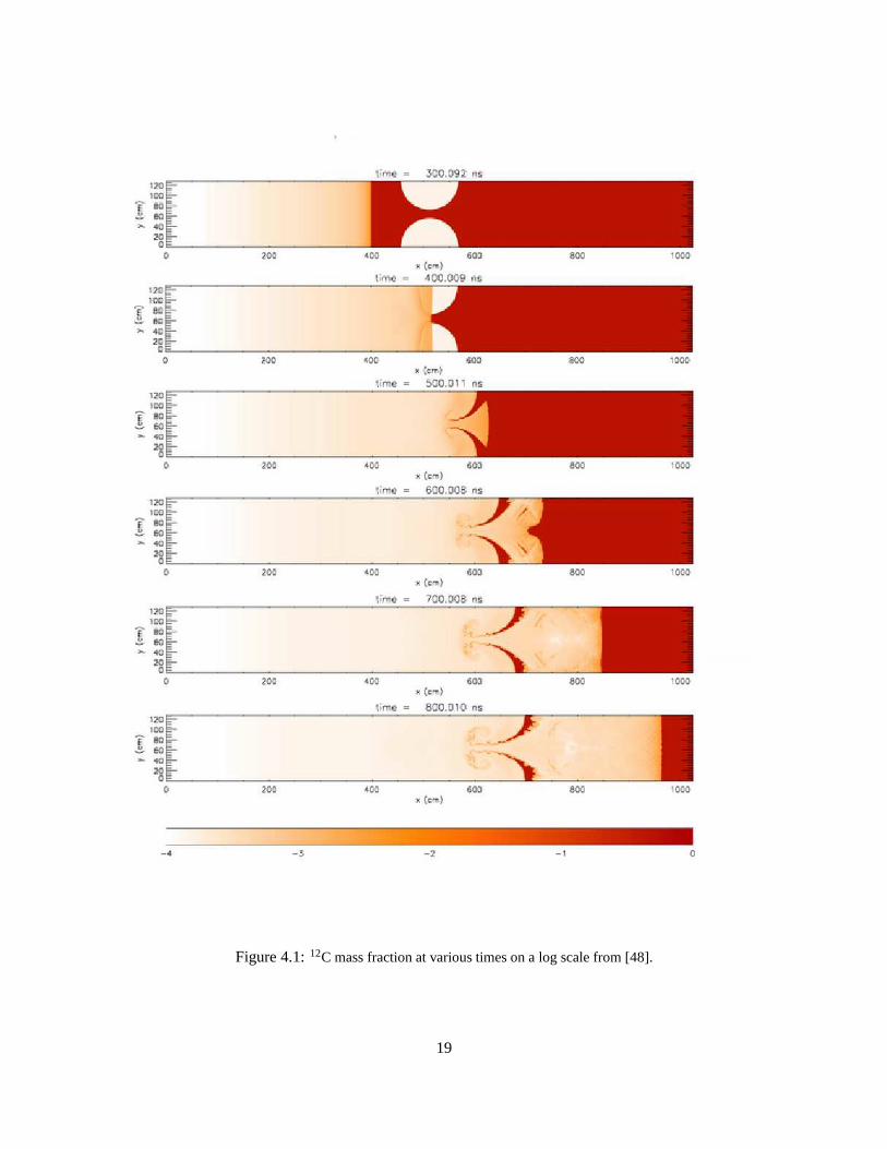
Figure 4.1:12C mass fraction at various times on a log scale from [48].
19

Figure 4.2: Initial temperature distribution using a logarithmic scale for the case withbarriers.
In this case, the instability forms as the burn front is passing through the constriction (Fig. 4.3-4.5)..
There are pockets of unburned material present well behind the burnfront which appears to be mixing with
the ash. Also, the shape of burn front appears to be somewhat different from what was seen in the Maier
paper, though this could be an effect of the lower resolutionwhich was used, in the present study. In the later
plots, the burn front has begun to reform into a plane wave. This is still well within the timeframe of the
Maier results, though the spatial region that is covered during this time is somewhat larger. Most likely this
is a result of starting the flame closer to the ash. Early testsshowed that when started from zero, the flame
had slowed significantly relative to the initial value, though it was still moving at a velocity well above the
speed of sound in the fuel (Fig. 4.6).
In a slightly different test, this one done with the same conditions on the Ash and Burn, but with the Fuel
at aT = 3×10⁹ K andρ = 1×10⁷gcm−3, the effects of interacting with ash that is slightly denserthan the
fuel is observed. This run was also started slightly furtherfrom the ash than the previous one. The left edge
here was defined as being at 300 cm with the Burn region again being 20 cm thick. The resolution of the
run was 7.5 cm. As can be seen from Fig. 4.8, the detonation front is compressed somewhat by the ash, but
not nearly to the extent seen in Fig. 4.1. The turbulence thatis seen in the Maier paper is almost completely
absent in these results, though that is to be expected: the Richtmeyer-Meshcov instability forms when the
detonation shock encounters a discontinuity in density [48]. The presence of the previously burned material
seems to have very little effect on the burn front. This is partially the result of the low resolution at which
the computation was run artificially smoothing out the system.
20

Figure 4.3:12C mass fraction at various times on a log scale.
21

Figure 4.4:12C mass fraction at various times on a log scale.
22
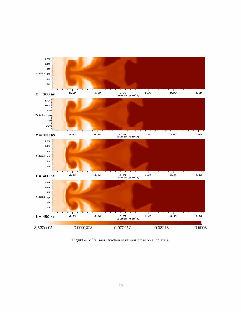
Figure 4.5:12C mass fraction at various times on a log scale.
23

Figure 4.6:Velocity in the x direction in units of cm s−1
Figure 4.7: Initial temperature distribution using a logarithmic scale for the case withhemispheres of ash.
24

Figure 4.8:12C mass fraction at various times on a log scale.
25

Table 4.2: Initial Conditions, 150 Isotope NetworkFuel Ash Burn
C12 0.5 0.0 0.5O16 0.5 0.0 0.5Ni56 0.0 1.0 0.0
T/109 K 0.01 5.505 10ρ /107 g cm−3 5.0 1.919 5.0dxdt /109 cm s−1 0.0 0.0 1.0
4.2 Results using 150-Isotope Network
After completing the low resolution test with the alpha network, we repeated the calculation with a larger
network. The run was done with the same resolution, but with slightly different parameters given in Table
4.2. The left edge was again set to be 420 cm and the width of theburn area 20 cm. It was originally
intended that the results of this run would be included in this thesis. Unfortunately, those computations have
not yet been completed.
In preparation for running the 150-isotope network for a situation more complicated than a single com-
putational cell, the FLASH code needed to be able to run on a massively parallel system. In this case,
the target machine was Eugene at the Oak Ridge National Laboratory (ORNL), an IBM BG/P. The basic
FLASH framework was able to run with only a few slight modifications that mainly involved finding the
correct compiler flags for the architecture. The additions which had been made by our group required more
work, as the code had to be updated to the Fortran 2003 standard which is used by the IBM XL compilers
on Eugene. After these corrections were made, FLASH was ableto run on Eugene. However, it was soon
discovered that the nuclear network which was being used wasbehaving incorrectly due to a fundamental
problem with the I/O routine. In our code, the nuclear network is read in from a text file that contains the
name, atomic mass, proton number, and neutron number for allthe isotopes to be used in a white space
delimited list. Due to an unresolved I/O bug on Eugene, the C-code that reads this file correctly stores the
proton and neutron number, but stores the wrong atomic mass.As one would expect, this results in serious
errors later on in the calculation, especially with the isotopes that are assigned a mass of zero. Because of the
problems that were encountered, it was decided to defer further work on the Eugene I/O problem until after
the completion of this thesis and, for the time being, to instead run on the multiple processor workstation
26

that was available. This lack of processing power was also the reason to run at a much lower resolution in
all of our cases.
The problem was setup and a run was started on the smaller machine (dual 3GHz processors). It was
at this point that the problem with the EOS that was mentionedduring the discussion of the approx13 runs
began to manifest itself. This problem results in the EOS routine being unable to correctly calculate the
internal energy for a zone. In the runs using the 150-isotopenetwork, there were no obvious indications
in the data that was output that a problem existed. The approx13 data did show that in certain zones on
the boundary between the ash and fuel the temperature would suddenly fall by several orders of magnitude.
This error did not occur when the initial temperature of the fuel was raised toT = 1×10⁹ K in the approx13
runs, but was still present in the 150-isotope calculations. Output from the code that deals with the nuclear
burning in bad zones indicates that the nuclear network is behaving in such a way that no obvious problem
could be found. This led to the conclusion that the error is with the equation of state itself, and is caused
by sharp discontinuities in the composition, since the temperature and densities present in the problem are
within the stated limits. Further tests have indicated thatthe error only occurs when a sharp discontinuity
in the composition occurs along with low temperatures. It ispossible that the problem is in fact related to
the resolution, and that the gradient in the composition is too large across those blocks. If higher levels of
refinement are allowed, the gradient would be less steep and the problem may be solved. This should be
possible once the I/O problem present on Eugene is resolved.Tests have been done on a single block that
is divided into two halves of the with the parameters for the fuel and ash as in the actual problem, but they
have been inconclusive (See Fig. 4.9).
27

Figure 4.9:Temperature plot from single block EOS test using the 150-isotope network.The left half is fuel and the right ash.
28

Chapter 5
Conclusions
At the end of any endeavor it is vital to take stock in what has been accomplished and what is still left to be
done.
5.1 Current Progress
• The calculations made with the approx13 network and ash hemispheres show that the behavior of
the detonation wave is qualitatively the same whether the algorithm used is the explicit asymptotic
method or the prescription used in the Maier & Niemeyer paper. This suggests that, the energies
being provided to the hydrodynamics code by our nuclear burning algorithm are similar to those in
the Maier and Niemeyer paper.
• Many of the changes necessary for running on larger computers such as the Eugene machine at Oak
Ridge National Labs have already been completed.
• While the calculation using the 150-isotope network has failed to run far enough to make any reason-
able conclusions as of the time this thesis was written, the problem has been defined and set up in
such as way that it could be easily run as soon as the problem with the EOS is resolved.
29

5.2 Future Work
• Currently, there has been little done in the way of optimizing the code. As much as a factor of ten
improvement may still be possible through numerical optimization and reorganization of the code.
Some preliminary tests suggest that larger increases in speed may be possible by the implementation
of newer explicit algorithms that are being developed to exploit the simplification that is implied by
the approach to equilibrium.
• It should be possible to have FLASH running with the explicit asymptotic burner on the Eugene
computer in a short amount of time. The only known problem currently preventing this is the error
with the code that reads in the nuclear network which is surely solvable.
• The EOS issue which was mentioned in the results section still needs to be resolved. More testing
should be done on small systems. So far the tests have all beendone with the ash being 100%
56Ni. The tests should be repeated with the ash at a compositionthat approximates nuclear statistical
equilibrium (NSE). Also, different boundary shapes need tobe tested, as well as the effect, if any, that
a change in resolution will have on the error.
• After FLASH coupled to the explicit asymptotic burner is working on Eugene, larger scale computa-
tions can then be carried out, an example being a run using theinitial conditions from the Maier paper
at full resolution (.4 cm) using the 150-isotope network. The ultimate goal is to be able to run the
simulation of a full star using a large network.
• Though many improvements remain to be made, current tests indicate that it should be possible to run
full scale simulations using a realistic network with the current version of the code in a reasonable
amount of time. The current barrier preventing this being the I/O problems that have been encoun-
tered.
30

Bibliography

Bibliography
[1] W. Hillebrandt and J.C. Niemeyer, Annu. Rev. Astron. Astrophys. 2000.38: 191–230
[2] B. Leibundgut, Annu. Rev. Astron. Astrophys. 2001.39: 67–90
[3] A.V. Fillipenko, Annu. Rev. Astron. Astrophys. 1997.35: 309–355
[4] W.D. Arnett. 1996. Supernovae and Nucleosynthesis. Princeton Univ. Press
[5] J.C. Niemeyer, J.W. Truran, eds. 1999. Type Ia Supernovae: Theory and Cosmology. Cambridge, UK:Cambridge Univ. Press
[6] M. Livio, N. Panagia, K. Sahu, eds. 2000. Supernovae and Gamma-Ray Bursts. Cambridge, UK:Cambridge Univ. Press
[7] P. Ruiz-Lapuente, R. Canal, J. Isern, eds. 1997. Thermonuclear Supernovae. Dordtecht, Ger.: Kluwer
[8] B. Leibundgut, Nuclear Physics,A688: 1c–8c, 2001
[9] B. Leibundgut, Computer Physics Communication147459–464, 2002
[10] J.L. Torny. et al., The Astrophysical Journal,594: 1–24, 2003 September 1
[11] B. Leibundgut, Astrophysics and Space Science290: 29–41, 2004
[12] S. Blinnikov, E. Sorokina, Astrophysics and Space Science290: 13–28, 2004
[13] A.G. Riess, et al., The Astronomical Journal,607: 665–687, 2004 June 1
[14] P.A. Pinto, R.G. Eastman, The Astrophysical Journal,530: 744-756, 2000, February 20
[15] L. Iapichino, M. Bruggen, W. Hillebrandt, and J.C. Niemeyer, Astronomy and Astrophysics,450:655–665, 2006
[16] T. Plewa, A.C. Calder, and D.Q. Lamb, The AstrophysicalJournal,612: L37-L40, 2004, Septermber1
[17] M.M. Phillips, The Astrophysical Journal Letters,413: L105–108, 1993
[18] B. Fryxell, et. al., The Astrophysical Journal Supplement Series,131: 273–334, 2000 November
[19] W. Hillebrandt, New Astronomy Reviews48: 615–621, 2004
32

[20] Vadim N. Gamezo, Alexei M. Khokhlov, and Elaine S. Oran,The Astrophysical Journal,623: 337–346, 2005, April 10
[21] E. Hairer, G. Wanner, Solving Ordinary Differential Equations II, (Stiff and Differential-AlgebraicProblems), 1991, Springer-Verlag, Berlin Heidelberg
[22] F.X. Timmes, The Astrophysical Journal Supplement Series,124: 241–263, 1999 September
[23] P. Colella, P.R. Woodward, J. Comp. Phys.,54: 172–201, 1984, September
[24] F.X. Timmes, and F.D Swesty, The Astrophysical JournalSupplement Series,126: 501–516, 2000February
[25] Mike Guidry, Kenneth J. Roche, Erin McMahon, and ReubenBudiardja, unpublished manuscript
[26] M.W. Guidry, O.E.B. Messer, and . Hix, and K.J. Roche, unpublished manuscript
[27] M.W. Guidry, R. Budiardja, E.Feger, W.R. Hix, O.E.B. Messer, and K.J. Roche, unpublishedmanuscript
[28] C. W. Gear,Numerical Initial Value Problems in Ordinary Differential Equations, Prentice Hall (1971)
[29] J. D. Lambert,Numerical Methods for Ordinary Differential Equations, Wiley (1991)
[30] W. H. Press, S. A. Teukolsky, W. T. Vettering, and B. P Flannery, Numerical Recipes in Fortran,Cambridge University Press (1992)
[31] E. S. Oran and J. P. Boris,Numerical Simulation of Reactive Flow, Cambridge University Press (2005)
[32] W. R. Hix and B. S. Meyer, to appear in special issue of Nuc. Phys. A; astro-ph/0509698
[33] T. Rauscher and F.-K. Thielemann, At. Data Nuclear DataTables75, 1 (2000)
[34] R. Hix and F.-K. Thielemann, J. Comp. Appl. Math.109, 321 (1999)
[35] M. Ruffert and H.-Th. Janka, Astrophysics and Astronomy, 380: 544–577, 2001
[36] A.M. Khokhlov, Journal of Computational Physics,143(2): 519–543, 1998
[37] F.K. Ropke, W.Hillebrandt, J.C Niemeyer, and S.E. Woosley, Astronomy and Astrophysics,448: 1–14,2006
[38] P.A. Mazzali, F.K. Ropke, S. Benetti, W. Hillenbrandt,Science,315: 825-828, 9 February 2007
[39] F.K. Ropke, and W.Hillebrandt, arXiv:astro-ph/0409286 v1 13 Sep 2004
[40] A.C. Calder, D.M. Townsley, I.R. Seitenzahl, F. Pang, O.E.B. Messer, N.Vladimirova, E.F. Brown,J.W. Truran, and D.Q. Lamb, The Astrophysical Journal,656: 313–332, 2007 February 10
[41] M. Zingale, S.E. Woosley, C.A. Rendleman, M.S. Day, andJ.B. Bell, The Astrophysical Journal,632:1021-1034, 2005, October 20
33

[42] L.D. Landau, E.M. Lifshitz (1959):Fluid Mechanics. vol. 6 of Course of Theoretical Physics, Perga-mon Press, Oxford
[43] M. Zingale, L.J. Dursi, The Astrophysical Journal,656: 333-346, 2007, February 10
[44] S.E. Woosley, S. Wunsch, M. Kuhlen. The Astrophysical Journal,607: 921-930, 2004, June 1
[45] V. Chupryna, ‘Explicit Methods in the Nuclear Burning Problem for Supernova Ia Models’(PhD Dis-sertation, University of Tennessee, Knoxville 2008)
[46] E. Feger, ’Evaluating a Flux=Limited Forward Differencing Method for Solving Large Physical Prob-lems’(PhD Proposal, University of Tennessee, Knoxville 2007)
[47] D.M. Townsley, A.C. Calder, S.M. Asida, I.R. Seitenzahl, F. Peng, N. Vladimirova, D.Q. Lamb, andJ.W. Truran, The Astrophysical Journal,668: 1118-1131, 2007 October 20
[48] A. Maier and J.C. Niemeyer, Astronomy and Astrophysics, 1-6, 1006
[49] M. Guidry, “Explicit Methods for Solutions of Large Thermonuclear Networks Coupled to Multidi-mensional Hydrodynamics Simulation”, unpublished manuscript
[50] G.C. Jordan IV, R.T. Fisher, D.M. Townsley, A.C. Calder, C. Graziani, S. Asida, D.Q. Lamb, J.W.Truran, The Astrophysical Journal, 2008
34
Vita
Christopher Ryan Smith was born in Shelbyville, Tennessee on October 22, 1985. He joined the Departmentof Physics and Astronomy as the University of Tennessee, Knoxville in 2002 as an undergraduate. He com-pleted his Bachelors of Science degree in May 2006, and stayed on to comtinue work towards a Masters.During his stay as a graduate student, he has worked as a Graduate Teaching Assistant teaching undergrad-uate physics and astronomy labs. He has done reasearch in thefield of astrophysics. He has completed hisMasters Degree in August 2009.
35


![Asymptotic behavior of singularly perturbed control …€¦ · Asymptotic behavior of singularly perturbed control ... [Lions, Papanicolau, Varadhan 1986]; ... Asymptotic behavior](https://static.fdocuments.in/doc/165x107/5b7c19bc7f8b9a9d078b9b98/asymptotic-behavior-of-singularly-perturbed-control-asymptotic-behavior-of-singularly.jpg)