WRLES: Wave Resolving Large-Eddy Simulation Code, Theory ...
Liu et al. / J Zhejiang Univ-Sci A (Appl Phys & Eng) 2018 19(12):904-925 904
Application of scale-resolving simulation to a hydraulic coupling,
a hydraulic retarder, and a hydraulic torque converter*
Chun-bao LIU†1,2, Jing LI1, Wei-yang BU1, Zhi-xuan XU1, Dong XU1, Wen-xing MA1,2 1School of Mechanical and Aerospace Engineering, Jilin University, Changchun 130022, China
2State Key Laboratory of Automotive Simulation and Control, Jilin University, Changchun 130022, China †E-mail: [email protected]
Received Sept. 21, 2017; Revision accepted Sept. 23, 2018; Crosschecked Nov. 10, 2018
Abstract: The paper describes the qualification and validation of large eddy simulation (LES) and hybrid Reynolds-averaged Navier–Stokes (RANS)/LES, the so-called scale-resolving simulation (SRS) approaches, which are currently employed in tran-sient simulations of internal flow for fluid machineries. Firstly, the application of various turbulence models in ANSYS FLUENT is briefly introduced to acquire the external performance of three hydrokinetic devices and to compare it with experimental data. It was found that a remarkable improvement in external performance was achieved. The best results could be as low as 4% for the absolute error in hydraulic coupling, 2%–5% for the error for the hydraulic retarder, and 2%–4% for the hydraulic torque con-verter. Basically, all models had better error levels than that of around 10%–15% obtained by RANS. Then four typical SRS simulations were applied to conduct numerical simulations of the internal flow fields for hydraulic coupling, the hydraulic re-tarder, and the hydraulic torque converter. The results provided two indisputable facts, firstly, that SRS models are more accurate in certain flow situations than RANS models and, secondly, that SRS models can give additional information compared with RANS simulations. Finally, the BSL SBES DSL model, a dynamic hybrid RANS/LES (DHRL) turbulence model, was applied to simulate and analyze the flow mechanism of the hydraulic coupling to deepen our understanding of it. The detailed flow structure in hydraulic coupling was determined and was used to understand the flow mechanism.
Key words: Scale-resolving simulation (SRS); Hybrid Reynolds-averaged Navier–Stokes (RANS)/large eddy simulation (LES);
Hydraulic coupling; Hydraulic retarder; Hydraulic torque converter https://doi.org/10.1631/jzus.A1700508 CLC number: TH137
1 Introduction
Hydraulic coupling, the hydraulic retarder, and
the hydraulic torque converter all belong to a set of
fluid machineries called hydrokinetic devices, using fluid kinetic energy to transmit power. They are widely applied in powertrain transmission systems, such as the use of hydraulic coupling in industrial energy saving, the hydraulic retarder in heavy trucks, and the torque converter in road or off-road vehicles and wheel loaders (Whitfield et al., 1978; Andersson, 1986; Hedman, 1992; Hampel et al., 2005). A hy-draulic coupling consists of a pump and a turbine, forming a mechanical device for transmitting rotary power. When the turbine is permanently braked, it functions as a hydraulic retarder, achieving retarda-tion by using the viscous drag forces between the pump and the turbine in a fluid-filled chamber. The-oretically, the torques of pump and turbine are always
Journal of Zhejiang University-SCIENCE A (Applied Physics & Engineering)
ISSN 1673-565X (Print); ISSN 1862-1775 (Online)
www.jzus.zju.edu.cn; www.springerlink.com
E-mail: [email protected]
* Project supported by the Key Scientific and Technological Project of Jilin Province (No. 20170204066GX), the Green Design Platform Construction Project for High-end Earthwork Machinery, Ministry of Industry and Information Technology, China (No. [2017]327), theOpen Foundation of Key Laboratory of Road Construction Technol-ogy and Equipment (Chang’an University), Ministry of Education ofChina (No. 310825171104), and the Advanced Manufacturing Pro-jects of Government and University Co-construction Program of JilinProvince, China (No. SXGJSF2017-2)
ORCID: Chun-bao LIU, https://orcid.org/0000-0002-8265-2875 © Zhejiang University and Springer-Verlag GmbH Germany, part of Springer Nature 2018

Liu et al. / J Zhejiang Univ-Sci A (Appl Phys & Eng) 2018 19(12):904-925 905
the same in hydraulic coupling. However, for the hydraulic torque converter, it is more of a fixed stator and can enlarge the input torque, which is the reason it is called a “torque converter”. The detailed division and relationship of the three hydraulic devices in the structure are shown in Fig. 1.
These three hydrokinetic devices possess ex-traordinarily complex 3D turbulent flows, which are unsteady, erratic, and composed of eddies. It is well known that the internal flows of fluid machines have a great influence on their overall performance. Although experimental methods, such as laser Doppler veloci-metry (LDV) or particle image velocimetry (PIV), can obtain information on the internal flows, there are still many difficulties in carrying out such studies because of the limitations of experimental conditions and cost considerations. Computational fluid dynamics (CFD) has been proposed to overcome the weakness of tra-ditional experimental methods (Zhang et al., 2016; Hu et al., 2017; Ji et al., 2017). In recent years, it has attracted increasing attention because of the possibil-ity of carrying out larger-scale research.
The CFD simulations in hydrokinetic devices were focused on not only performance prediction, but also on visually displaying the rotor-stator interaction and eddy viscosity structures. When the performance prediction was within the accuracy achievable in the analysis, it could reach a level permitting design solely based on computational results. Thus, a series of numerical simulation models were proposed based on different solving methods for resolving governing equations. The Reynolds-averaged Navier–Stokes
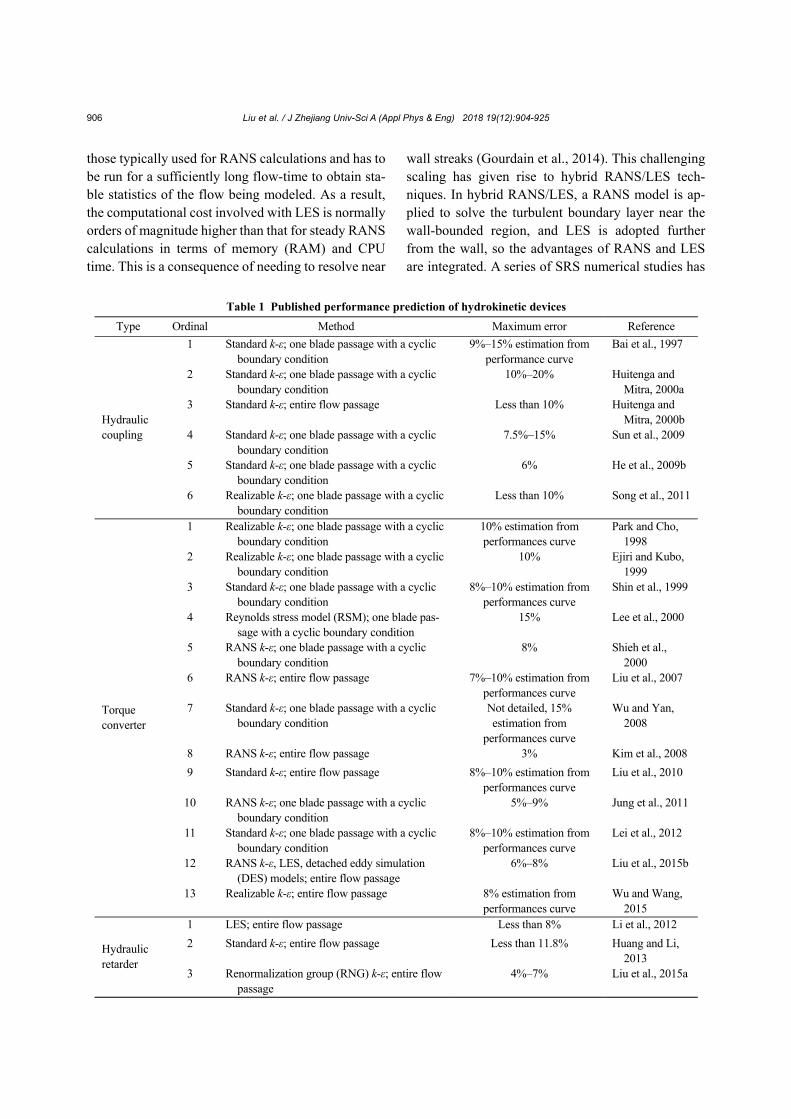
(RANS) equations were most widely used in indus-trial flows. The large eddy simulation (LES) and hybrid LES/RANS methods, the so-called scale- resolving simulation (SRS), which could partially resolve the flow field, have been applied in industrial flows successfully (Gritskevich et al., 2014). The numerical simulation of the flow field for a hydraulic torque converter started with the studies of Laksh-minarayana (1991) and Schulz et al. (1996). Inspired by the study of Denton (1986), the whole 3D, in-compressible, unsteady flow was calculated via the mixing plane, which was used to interact between adjacent impellers. Flack and Brun (2003) simulated the unsteady flow in a torque converter with the LES method. Kim et al. (2008) made a performance esti-mation model for a torque converter using the corre-lation between the internal flow field and the energy loss coefficient. Jung et al. (2011) performed a com-parative study to investigate the effect of different methods (the frozen rotor, sliding mesh, and mixing plane methods) for handling the interaction of im-pellers. The CFD simulation had showed the potential to improve performance prediction (Li et al., 2012; Liu et al., 2015b) and gradually became an effective tool integrated into the converter’s design process. A review of the CFD applications in hydraulic coupling, hydraulic retarder, and hydraulic torque converter is shown in Table 1.
It was obvious that CFD simulations for the three hydrokinetic devices were mainly based on the RANS turbulence models. However, there are two main disadvantages in using RANS models. The first is the additional information that cannot be obtained from the RANS simulation and the second is related to simulation accuracy. It is well known that RANS models have limitations in accuracy in certain flow situations. The idea behind the RANS equations was Reynolds decomposition, whereby an instantaneous quantity was decomposed into time-averaged and fluctuating quantities, so unsteady flow information would be eliminated during calculation. Certain classes of turbulence models, termed SRS, including LES and hybrid RANS/LES, cover all or a part of the turbulence spectrum in at least a portion of the nu-merical domain. In LES, large eddies are resolved directly, while small eddies are modeled. However, LES still requires substantially finer meshes than
Fig. 1 Classification and relationship of three hydrokinetic devices
Rot
ated
Fix
ed
Fix
ed
Rot
ated
Rot
ated
Ro
tate
d
Ro
tate
d
Liu et al. / J Zhejiang Univ-Sci A (Appl Phys & Eng) 2018 19(12):904-925 906
those typically used for RANS calculations and has to be run for a sufficiently long flow-time to obtain sta-ble statistics of the flow being modeled. As a result, the computational cost involved with LES is normally orders of magnitude higher than that for steady RANS calculations in terms of memory (RAM) and CPU time. This is a consequence of needing to resolve near
wall streaks (Gourdain et al., 2014). This challenging scaling has given rise to hybrid RANS/LES tech-niques. In hybrid RANS/LES, a RANS model is ap-plied to solve the turbulent boundary layer near the wall-bounded region, and LES is adopted further from the wall, so the advantages of RANS and LES are integrated. A series of SRS numerical studies has
Table 1 Published performance prediction of hydrokinetic devices
Type Ordinal Method Maximum error Reference
Hydraulic coupling
1 Standard k-ε; one blade passage with a cyclic boundary condition
9%–15% estimation from performance curve
Bai et al., 1997
2 Standard k-ε; one blade passage with a cyclic boundary condition
10%–20% Huitenga and Mitra, 2000a
3 Standard k-ε; entire flow passage Less than 10% Huitenga and Mitra, 2000b
4 Standard k-ε; one blade passage with a cyclic boundary condition
7.5%–15% Sun et al., 2009
5 Standard k-ε; one blade passage with a cyclic boundary condition
6% He et al., 2009b
6 Realizable k-ε; one blade passage with a cyclic boundary condition
Less than 10% Song et al., 2011
Torque converter
1 Realizable k-ε; one blade passage with a cyclic boundary condition
10% estimation from performances curve
Park and Cho, 1998
2 Realizable k-ε; one blade passage with a cyclic boundary condition
10% Ejiri and Kubo, 1999
3 Standard k-ε; one blade passage with a cyclic boundary condition
8%–10% estimation from performances curve
Shin et al., 1999
4 Reynolds stress model (RSM); one blade pas-sage with a cyclic boundary condition
15% Lee et al., 2000
5 RANS k-ε; one blade passage with a cyclic boundary condition
8% Shieh et al., 2000
6 RANS k-ε; entire flow passage 7%–10% estimation from performances curve
Liu et al., 2007
7 Standard k-ε; one blade passage with a cyclic boundary condition
Not detailed, 15% estimation from
performances curve
Wu and Yan, 2008
8 RANS k-ε; entire flow passage 3% Kim et al., 2008
9 Standard k-ε; entire flow passage 8%–10% estimation from performances curve
Liu et al., 2010
10 RANS k-ε; one blade passage with a cyclic boundary condition
5%–9% Jung et al., 2011
11 Standard k-ε; one blade passage with a cyclic boundary condition
8%–10% estimation from performances curve
Lei et al., 2012
12 RANS k-ε, LES, detached eddy simulation (DES) models; entire flow passage
6%–8% Liu et al., 2015b
13 Realizable k-ε; entire flow passage 8% estimation from performances curve
Wu and Wang, 2015
Hydraulic retarder
1 LES; entire flow passage Less than 8% Li et al., 2012
2 Standard k-ε; entire flow passage Less than 11.8% Huang and Li, 2013
3 Renormalization group (RNG) k-ε; entire flow passage
4%–7% Liu et al., 2015a

Liu et al. / J Zhejiang Univ-Sci A (Appl Phys & Eng) 2018 19(12):904-925 907
been conducted by Tucker (2011a, 2011b, 2013) to investigate turbomachinery flows. Reviews of LES and related approaches in turbomachinery are also given by Menzies (2009), Denton (2010), Duchaine et al. (2013), Tyacke et al. (2014), and Yang (2015). Tucker et al. (2012a, 2012b) pointed out that hybrid RANS/LES and LES seem to have an equal but subservient frequency of use in turbomachinery applications. It became increasingly clear that many researchers have recognized the potential advantages of SRS simulations and have conducted studies on industrial flows.
The development and application of SRS simu-lations, including LES and hybrid RANS/LES, should therefore be the trend in flow simulation for these hydrokinetic devices. However, it was apparent that application of turbulence models did not match the rapid development of turbulence models themselves. Recognizing that fact, a series of comprehensive SRS calculations for the three hydrokinetic devices was carried out and is described in this paper. Our objec-tives were very clear. Firstly, we did meticulous work in summarizing and classifying the turbulence models in a commercial software, ANSYS FLUENT, which was significant for better understanding the applica-tion of turbulence models. Then we undertook the second, most important, stage and the three hydroki-netic devices, hydraulic coupling, hydraulic retarder, and hydraulic torque converter, were used to respec-tively conduct the numerical simulations in a series of SRS models, which were synthetically assessed by quantitative and qualitative analysis. Hence, the po-tential strength of SRS simulations compared with RANS simulations, was demonstrated and the choice of the turbulence models to be applied to industrial flow is made considerably easier than before. 2 Numerical simulation
Basically, fluid flow is governed by the laws of
physical conservation, including mass conservation, momentum conservation, and energy conservation. The conservation laws are mathematically described by the governing equations, which can be expressed as follows.
Continuity equation is
0.i
i
u
t x
(1)
Momentum equation is
.
i ji ii
j j j
u uu uS
t x x x
(2)
Energy equation is
.
ij
j j j ij hjj
Eu E p
t x
Th J u S
x x
(3)
In Eqs. (1)–(3), ρ is the fluid density, t is the
time, ui is the velocity component, Si is the source item, μ is the dynamic viscosity, E is the unit mass energy, p is the pressure, λ is the thermal conductivity, T is the temperature, hj is the enthalpy component, Jj is the diffusion flux component, τij is the viscous stress tensor, and Sh is the viscous dissipation term.
It is not very realistic to directly solve turbulent pulsation characteristics through governing equa-tions. There are more stringent requirements for spa-tial and temporal solutions to obtain the flow infor-mation at all scales which require a lot of computation which is time-consuming and has strong dependence on computer memory. To deal with this problem, it is recognized that some approximation and simplifica-tion for turbulence must be made by introducing a different turbulence method. This method of numer-ical simulation of turbulence is described as non- direct numerical simulation.
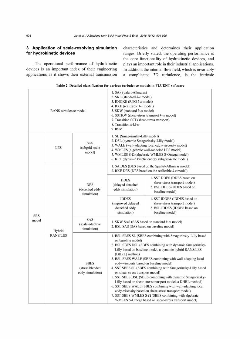
The non-direct numerical simulation consists of LES, statistical average simulation, and RANS. The statistical average simulation is based on the statisti-cal theory of correlation function mainly by applying the correlation function and spectral analysis to study the turbulent structure. The statistical theory is mainly concerned with the application of small scale eddies, so it is not widely used in engineering. In the study, FLUENT software is applied to carry out the numer-ical simulation, and the detailed classification for various turbulence models is shown in Table 2.
Liu et al. / J Zhejiang Univ-Sci A (Appl Phys & Eng) 2018 19(12):904-925 908
3 Application of scale-resolving simulation for hydrokinetic devices
The operational performance of hydrokinetic
devices is an important index of their engineering applications as it shows their external transmission
characteristics and determines their application ranges. Briefly stated, the operating performance is the core functionality of hydrokinetic devices, and plays an important role in their industrial applications. In addition, the internal flow field, which is invariably a complicated 3D turbulence, is the intrinsic
Table 2 Detailed classification for various turbulence models in FLUENT software
RANS turbulence model
1. SA (Spalart-Allmaras) 2. SKE (standard k-ε model) 3. RNGKE (RNG k-ε model) 4. RKE (realizable k-ε model) 5. SKW (standard k-ɷ model) 6. SSTKW (shear-stress transport k-ɷ model) 7. Transition SST (shear-stress transport) 8. Transition k-kl-ɷ 9. RSM
SRS model
LES SGS
(subgrid-scale model)
1. SL (Smagorinsky-Lilly model) 2. DSL (dynamic Smagorinsky-Lilly model) 3. WALE (wall-adapting local eddy-viscosity model) 4. WMLES (algebraic wall-modeled LES model) 5. WMLES S-Ω (algebraic WMLES S-Omega model) 6. KET (dynamic kinetic energy subgrid-scale model)
Hybrid RANS/LES
DES (detached eddy
simulation)
1. SA DES (DES based on the Spalart-Allmaras model) 2. RKE DES (DES based on the realizable k-ε model)
DDES (delayed detached eddy simulation)
1. SST DDES (DDES based on shear-stress transport model)
2. BSL DDES (DDES based on baseline model)
IDDES (improved delayed
detached eddy simulation)
1. SST IDDES (IDDES based on shear-stress transport model)
2. BSL IDDES (IDDES based on baseline model)
SAS (scale-adaptive
simulation)
1. SKW SAS (SAS based on standard k-ɷ model) 2. BSL SAS (SAS based on baseline model)
SBES (stress blended
eddy simulation)
1. BSL SBES SL (SBES combining with Smagorinsky-Lilly based on baseline model)
2. BSL SBES DSL (SBES combining with dynamic Smagorinsky- Lilly based on baseline model, a dynamic hybrid RANS/LES (DHRL) method)
3. BSL SBES WALE (SBES combining with wall-adapting local eddy-viscosity based on baseline model)
4. SST SBES SL (SBES combining with Smagorinsky-Lilly based on shear-stress transport model)
5. SST SBES DSL (SBES combining with dynamic Smagorinsky- Lilly based on shear-stress transport model, a DHRL method)
6. SST SBES WALE (SBES combining with wall-adapting local eddy-viscosity based on shear-stress transport model)
7. SST SBES WMLES S-Ω (SBES combining with algebraic WMLES S-Omega based on shear-stress transport model)

Liu et al. / J Zhejiang Univ-Sci A (Appl Phys & Eng) 2018 19(12):904-925 909
embodiment of hydrokinetic devices. Nowadays, CFD technology combined with experimental meas-urements is widely applied in the design of hydroki-netic devices and has proved an effective method. In this study, three typical hydrokinetic devices, hy-draulic coupling, hydraulic retarder, and hydraulic torque converter, are selected as study objects for performing theoretical analysis including perfor-mance prediction and flow visualization by CFD numerical simulation.
3.1 Experiment and equipment
3.1.1 Measurement of 3D geometry
The 3D laser scanner is the one of the best scanning systems for measuring speed and accuracy, possessing unique advantages of high efficiency and high precision, especially for complex surfaces. Here, a typical 3D scanner is applied to accurately perform the structural measurement and reconstruction of hydrokinetic devices as shown in Fig. 2.
Before measurement, it is necessary to uni-
formly spray the imaging agent on the surface of the hydrokinetic devices, and then to place a small black circle as reference point. When this step is completed, the next is to place the processed devices on the worktable and adjust the position and angle of the scanner. Finally, the 3D geometric files of the hy-drokinetic devices can be obtained through software processing.
3.1.2 Test rig for external performance
For stator-rotor machines, quantitative external characteristics are mostly determined by the average effect of internal flow field on the impellers. Theo-
retically, consistency of external characteristics in-volving numerical simulation and bench tests can prove the validity of the numerical simulation method indirectly so as to analyze the flow field in hydroki-netic devices.
On the basis of test requirements, a hydraulic transmission test rig was built to test the hydrokinetic devices for external performance. The hydraulic transmission test rig consists of three parts: the main test part, the oil supply system, and the control and data acquisition systems. The main test part of the rig includes a drive dynamometer, the hydraulic device, a torque-speed transducer, and an absorption dyna-mometer. The drive dynamometer is the power device and the absorption dynamometer is the loading device of the test rig, and they determine the parameters required for the test. The hydraulic transmission test rig and its schematic diagram are shown in Fig. 3.
For the three hydrokinetic devices, the test rig is able to be operated to obtain the different external data by simply changing the hydrokinetic device without any other structural adjustment. Therefore, all quantitative external performance data involved in the following are specially obtained from bench tests.
Fig. 2 Three-dimensional laser scanner (a) Scanner; (b) Measuring module; (c) Orientation module
Fig. 3 Test rig of hydraulic transmission (a) and its sche-matic diagram (b) 1: drive dynamometer; 2: hydraulic device; 3: torque-speedtransducer; 4: absorption dynamometer; 5: computer; 6: signalconversion card; 7: control cubicle; 8: oil circuit controller; 9:pump station; 10: heat exchanger
(a)
(b)

Liu et al. / J Zhejiang Univ-Sci A (Appl Phys & Eng) 2018 19(12):904-925 910
3.2 Hydraulic coupling
3.2.1 Computational model and grid partition
Hydraulic coupling consists of a pump and a turbine, for which detailed geometrical parameters can be accurately obtained by the 3D scanning tech-nique. Based on the measured results, the structural data are shown in Table 3.
Then, the 3D model of hydraulic coupling can be constructed accurately by modeling software based on measurement data, as shown in Fig. 4a. As the basis for grid partition, the computational domain was also established, which indicated the region of fluid motion, as shown in Fig. 4b.
Theoretically, a structured grid has many ad-vantages, such as simple structure, fast generation, and good grid quality. It is strongly recommended when the computation model is relatively simple. In addition, the hydraulic coupling, namely YH380 with simple flat torus and blades, is fairly suitable for generating high quality meshes for performing a re-liable numerical simulation. Thus, in order to guar-antee computational accuracy and to reduce the cal-culation time, the structured hexahedral grid for the entire computational domain was generated pro-grammatically by ANSYS ICEM, and the cluster points were placed at the boundary layer to refine the mesh by specifying the node number and distribution principle for the near wall region. The grid model of hydraulic coupling is shown in Fig. 4c.
3.2.2 Numerical simulation and verification of grid independence
Reasonable solution setting is the premise for obtaining reliable simulation results, and special at-tention should be paid to avoid irrational procedural errors during the numerical simulation process. Recognizing their importance, some non-negligible computational conditions are listed in Table 4.
For the transient solution, the time step Δt must
be small enough to resolve time-dependent charac-teristics, and can be estimated roughly by
,x
tv
(4)
where Δx is the local grid size, and v is the charac-teristic flow velocity.
Considering the grid sizes of different partitions and the characteristic velocity of the flow field, the time step was defined as 0.0002 s and the number of steps was 750, so the total computation time was 0.15 s. In order to ensure the accuracy of the calcula-tion results, the torque and residual curves were monitored. The calculation results were considered to have converged when the change rate for torque values in two consecutive iterations was less than 10−4, and all normalized residual values in Navier– Stokes (N-S) equations were less than 10−6.
The verification of grid dependence was also essential to eliminate the influence of grid density on the calculation results, and thereby to increase the accuracy and reliability of the calculation results. Thus, before the CFD calculation, the LES model was applied to conduct a numerical simulation for the grid
Table 3 Geometrical parameters of hydraulic coupling
Parameter Description
Pump Turbine
Effective diameter of circle (mm) 380 380
Number of blades 12 10
Thickness of blades (mm) 5 5
Type of blades Straight Straight
Table 4 Boundary settings during numerical simulation
Analysis type Transient state Solver type Pressure-based
Momentum Bounded central differencing
Transient formulation Second-order implicit
Interaction Sliding mesh
Pressure-velocity coupling SIMPLEC
Pump status Rotate
Turbine status Static
Viscosity (Pas) 0.0258
Density (kg/m3) 860
SIMPLEC: semi-implicit method for pressure-linked equations consistent
Fig. 4 Establishment of the 3D model and division of gridmodel of hydraulic coupling (a) Physical model; (b) Computational domain; (c) Grid layout

Liu et al. / J Zhejiang Univ-Sci A (Appl Phys & Eng) 2018 19(12):904-925 911
dependence involving absolute braking error and computation time, and the results are shown in Fig. 5. Considering the prediction accuracy and computation time, the grid cell number for the entire flow passage was chosen to be 6 million.
3.2.3 Results and analysis
Here, a full range of turbulence models, includ-ing RANS, LES, and hybrid RANS/LES, were ap-plied to calculate the unsteady flow field to assess the effectiveness of flow structure description and per-formance prediction. On this basis, we can gain a clearer understanding of the potential strengths of SRS models by comprehensive comparison with RANS models. 3.2.3.1 External performance
The absolute errors of braking torque were the typical operating performance in hydraulic coupling. Here, the typical results in full charging ratio and different rotation speeds obtained by experimental test and CFD simulation are shown in Fig. 6. There were four categories. One was RANS and the others were SRS approaches. Generally, there was a similar error distribution trend for these turbulence models, as detailed below.
At low speeds, the experimental results were very sensitive to the operating environment and ex-perimental conditions. In addition, due to the influ-ence of other factors such as weak centrifugal force and insufficient flow, the predicted errors had a rela-tively large fluctuation. However, with the increase in rotation speeds, the proportion of the centrifugal force increased and the flow developed fully. Therefore, other factors can be ignored and the simulation con-
ditions were approaching the ideal situation (John-ston, 1998), which was not affected by the external environment, resulting in the absolute errors between numerical simulation and experimental data gradually decreasing. The overall tendency was in accordance with the theoretical basis.
Based on detailed analysis, the different abilities of prediction for various turbulence models were demonstrated clearly at a rotating speed of 600 r/min. The errors for RANS methods were in a larger range, about 7.5%–11%, which was consistent with the theory that the limitations of RANS models would not allow them to achieve higher accuracy in certain flow situations. For the SRS simulations, accuracy was sig-nificantly improved: the maximum error was less than 9%, and the minimum error was as low as 4%. Based on the above analysis, it can be seen that, on the one hand, the SRS simulations have some advantages in prediction accuracy and, on the other, they were strong performers in numerical simulation of the hydraulic coupling. Thus, the internal flow field of the hydraulic coupling was conducted and analyzed in detail. 3.2.3.2 y+ distribution
The dimensionless term y+ was mainly applied to partition the boundary layer of turbulence, which could qualitatively identify the ability of various turbulence models to solve the near-wall region. The near-wall treatments consisted of two approaches: applying wall functions and resolving the viscous sublayer. Usually a high-density mesh is a mandatory condition for the near-wall region to be able to resolve the viscous sublayer on which additional information is indispensable for some wall-bounded flows. On the other hand, if a coarse mesh was used, the wall pro-vides an approximate treatment method that can be employed for an alternative solution. Fig. 7 shows the y+ distribution in the pressure sides of the pump and turbine. It was clear that the distribution trends for all turbulence models were similar in general. Never-theless, it was undeniable that the y+ magnitude of RANS models was relatively large, especially the k-ε models, indicating that the RANS models have their limitations in resolving wall-bounded flow despite of the use of the wall functions. By comparison, it was obvious that the SRS models were stronger. There-fore, they are increasingly recommended for applica-tion in cases where the wall-bounded flows have an important influence on the simulation results.
Fig. 5 Verification of grid independence

Liu et al. / J Zhejiang Univ-Sci A (Appl Phys & Eng) 2018 19(12):904-925 912
Fig. 6 Absolute error of braking torque under different turbulence models
Fig. 7 y+ distribution in pressure sides of pump and turbine
Liu et al. / J Zhejiang Univ-Sci A (Appl Phys & Eng) 2018 19(12):904-925 913
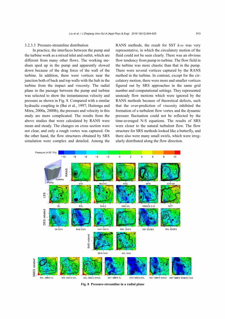
3.2.3.3 Pressure-streamline distribution In practice, the interfaces between the pump and
the turbine work as a mixed inlet and outlet, which are different from many other flows. The working me-dium sped up in the pump and apparently slowed down because of the drag force of the wall of the turbine. In addition, there were vortices near the junction both of back and top walls with the hub in the turbine from the impact and viscosity. The radial plane in the passage between the pump and turbine was selected to show the instantaneous velocity and pressure as shown in Fig. 8. Compared with a similar hydraulic coupling in (Bai et al., 1997; Huitenga and Mitra, 2000a, 2000b), the pressure and velocity in this study are more complicated. The results from the above studies that were calculated by RANS were mean and steady. The changes on cross section were not clear, and only a rough vortex was captured. On the other hand, the flow structures obtained by SRS simulation were complex and detailed. Among the
RANS methods, the result for SST k-ω was very representative, in which the circulatory motion of the fluid could not be seen clearly. There was an obvious flow tendency from pump to turbine. The flow field in the turbine was more chaotic than that in the pump. There were several vortices captured by the RANS method in the turbine. In contrast, except for the cir-culatory motion, there were more and smaller vortices figured out by SRS approaches in the same grid number and computational settings. They represented unsteady flow motions which were ignored by the RANS methods because of theoretical defects, such that the over-prediction of viscosity inhibited the formation of a turbulent flow vortex and the dynamic pressure fluctuation could not be reflected by the time-averaged N-S equations. The results of SRS were closer to the natural turbulent flow. The flow structure for SRS methods looked like a butterfly, and there also were many small swirls, which were irreg-ularly distributed along the flow direction.
Fig. 8 Pressure-streamline in a radial plane
−10 −8 −6 −4 −2 0 2 4 6 8 10

Liu et al. / J Zhejiang Univ-Sci A (Appl Phys & Eng) 2018 19(12):904-925 914
In addition, there was a very interesting flow phenomenon, which was that low pressure appeared in some methods. It should be realized that this was a 3D flow. The local pressure regions were the core of 3D vortex structures and the magnitudes of the vorti-city in these regions were lower. They were important for understanding the evolution of the vortex and the structural features during energy transmission be-tween pump and turbine. This transient flow phe-nomenon could only be captured by SRS approaches. 3.2.3.4 Vortex structure
Further analysis is required to reveal the detailed processes of energy transmission between pump and turbine. Therefore, several typical SRS methods, KET, SST DDES, BSL SAS, and BSL SBES DSL, were applied to conduct further analysis for the three hydrokinetic devices.
In the flow field, the essential characteristics for turbulence were the formation of the vortex, and its diffusion and dissipation. Therefore, the key to ana-lyzing the flow field by the turbulence model was to describe the vortex structures (Wu et al., 2011). Q-criterion was introduced to capture the vortex structure under 600 r/min in the flow field. Fig. 9 shows the vortex structures as a whole from a front view of the pump. The vortices were concentrated in the region from the hub to one-third blade height, where the kinetic energy of fluid transmission took place. If the engineer wants to improve the perfor-mance by controlling the flow field and boundary, as in (Huitenga and Mitra, 2000a, 2000b), some signif-icant places needed to focus on, which inspired di-rectly and avoided the attempts. The models all gave rich vortices and could hardly be differentiated by qualitative analysis.
Following from the above, we focused on this region and made a serious effort to analyze the vortex flow patterns and processes as shown in Fig. 10. The target region is shown in the lower left corner of the picture. It includes two blade passages. The pump was located outside and the turbine was inside. The left and right red arrows show the theoretical flow direc-tions in the pump and turbine, respectively, and the blue ones show the circulating flow track between the pump and turbine. A black arrow revolving around Z axis represents the direction of rotation. As seen from the figure, each model has a main picture and four subsidiary enlarged ones. Among them, the upper left
shows the vortex along the turbine blade and the lower left shows the flow from turbine to pump, the lower right shows the main vortices from pump to turbine and the upper right shows the vortex forming in the turbine blade by instantaneous shocks.
3.2.3.5 Quantitative analysis
Some control points placed in a section of the turbine channel were then qualitatively monitored for data statistics including velocity, pressure, and tur-bulent kinetic energy (TKE) to further elaborate the flow mechanism. Fig. 11 shows the positions of the control points, which were equidistant 5 mm.
It is well known that the distribution character-istics of velocity and pressure are the typical mani-festation of the internal flow fields of rotating ma-chinery. Thus, it was very necessary to conduct the data statistics for internal flow fields so as to quantify the complex 3D turbulence as shown in Fig. 12. Through the quantitative analysis of velocity and pressure, it can be clearly seen that the loss in the middle length of the chord is obviously because of the impact of the fluid on the wall. The TKE is a measure of the development or decline of turbulence. The KET did not model the TKE, so the TKE is not shown for this model. Obviously, BSL SAS overestimated the
Fig. 9 Vortex structure in pump
Fig. 10 Vortex structures in channel of pump and turbineFor interpretation of the references to color in this figure, thereader is referred to the web version of this article

Liu et al. / J Zhejiang Univ-Sci A (Appl Phys & Eng) 2018 19(12):904-925 915
turbulence in the flow region, which resulted in errors in performance prediction. However, SST DDES and BSL SBES DSL behaved consistently in predicting TKE. The fluid was attached to the near wall due to viscosity and thus energy was consumed. Compre-hensively, BSL SBES DSL had a strong predictive advantage in the prediction of turbulence.
3.3 Hydraulic retarder
3.3.1 Computational model and grid partition
A hydraulic retarder can be regarded as the spe-cific hydraulic coupling playing a role in braking. Similarly, the geometric parameters of the hydraulic retarder are listed in Table 5, which can be obtained by advanced measurement technology. The ho-lonomic 3D model of the hydraulic retarder is shown in Fig. 13a.
Mesh generation is a crucial step in numerical simulation by the finite volume method, and directly affects the accuracy of subsequent numerical analy-sis. Therefore, hexahedral structured grids for the whole passage were generated for performing the numerical calculation for the N-S equations. Both the computational domain model and structured grid model are shown in Figs. 13b and 13c.
Table 5 Geometrical parameters of hydraulic retarder
Parameter Description
Rotor Stator Effective diameter of circle (mm) 296 293
Number of blades 38 36
Type of blades Straight Straight
Anteversion angle of blades (°) 40 40
Wedge angle of blades (°) 30 30
Number of inlets 0 12
Number of outlets 0 6
Fig. 13 Establishment of the 3D model and division of gridmodel of hydraulic retarder (a) Physical model; (b) Computational domain; (c) Grid layout
Fig. 11 Placement of control points (H and h are theheights of the blade and control points, respectively)
Fig. 12 Statistical results of four turbulence models (a) Velocity; (b) Pressure; (c) TKE
Z position (mm)
Z position (mm)
Z position (mm)

Liu et al. / J Zhejiang Univ-Sci A (Appl Phys & Eng) 2018 19(12):904-925 916
3.3.2 Numerical simulation and verification of grid independence
ANASYS FLUENT, as a professional CFD software, was employed to conduct the numerical simulation for solving the physical quantities in tur-bulent flow. The specific boundary conditions were set according to Table 6.
During the calculation, the outlet pressure and
braking torque were monitored. The solution was assumed to have converged when all residuals of mass and momentum were less than 10−6, and the results of outlet pressure and braking torque in two circulatory iterations were consistent.
Before the formal numerical simulation, a mesh sensitivity test had been carried out to minimize the effect of grid number. Based on the analysis results as shown in Fig. 14, and considering the calculation precision and computation time, the grid cell numbers of the rotor and the stator were set at 1.44 million and 1.61 million, respectively.
3.3.3 Results and analysis
3.3.3.1 External performance The rig test was carried out to acquire the brak-
ing torques at different filling rates and different speeds, and the simulated braking torque values were extracted and compared with the experimental values. Comparison between the experimental and predicted results is shown in Fig. 15. Overall, the predicted results for four turbulence models were in good agreement with the experimental data. The maximum and minimum errors were 9.66% and 2.24%, respec-tively. These four turbulence models are therefore
reliable for numerical simulation of the hydraulic retarder.
3.3.3.2 Velocity distribution
It was clear that the internal flow in a hydraulic retarder was a complex 3D movement of revolving turbulence. The section of a torus was selected as reference surface to further analyze the velocity dis-tribution under different turbulence models, as shown in Fig. 16.
The observations in the figure indicate that the transient velocity distribution at the section is basi-cally consistent during the same time period under four turbulence models. The transmission oil in the rotor was accelerated under the action of centrifugal force, achieving maximum velocity at the exit of the outer loop region. The arrest of the stationary blades
Fig. 15 Comparison between experimental and predictedresults for braking torque (a) Liquid filling rate q=100%; (b) Liquid filling rate q=50%
Table 6 Boundary settings during numerical simulation
Analysis type Transient state Solver type Pressure-based
Inlet Velocity-inlet
Outlet Outflow
Interaction Sliding mesh
Pressure discretization PRESTO
Pressure-velocity coupling PISO
Transient formulation Second order implicit
Time step size 0.0005 s
Number of time steps 1200
PRESTO: pressure staggering option; PISO: pressure implicit with splitting operators
Fig. 14 Verification of grid independence

Liu et al. / J Zhejiang Univ-Sci A (Appl Phys & Eng) 2018 19(12):904-925 917
impeded the directional flow in the stator, resulting in a deceleration. There was a special phenomenon: the velocity was somewhat modified at the exit of the stator passage because of the agitation of the rotor. In addition, the blocking action when a high-speed fluid impacted the blades and the outer ring of the stator, led to a large velocity gradient and the formation of a low-speed vortex at the center of the torus (He et al., 2009a). In spite of the consistency of the overall ve-locity distribution in the four models, there were still some differences in the details. It was obvious that the velocity gradient was relatively large at half a circle for the KET model indicating energy loss was rela-tively large, but the prediction results of other models were basically consistent. Briefly, the four turbulence models had better prediction results for velocity distribution.
3.3.3.3 Pressure distribution The pressure distribution in the blades of the
hydraulic retarder is reflected in Fig. 17. On the whole, the pressure contour lines are distributed along the posterior wall. There were three main factors influencing the change of pressure (Wang et al., 2012): centrifugal force, relative velocity, and vis-cosity. When the speed of the rotor is constant, the effect of centrifugal force remains unchanged. At high speed, the effect of relative velocity and viscos-ity on the change of pressure is lower than that of the centrifugal force. Therefore, the role of centrifugal force becomes more and more significant, and shows a distribution trend along the radial direction.
For the rotor, the centrifugal force of the fluid flow makes the high pressure appear at the root of blade. For the stator, the high pressure area is rela-tively large because of the blocking effect of the blades, and the low pressure area is caused by the generation of a wake when the fluid flow directly
impacts the pressure surface. The inlet was in the low pressure area of the stator, which ensured that the fluid entered the working chamber at high speed. The location of the maximum value is close to the position where the transmission oil directly impacts the stator blades.
3.3.3.4 Rothalpy distribution In the hydraulic retarder, the hydraulic loss is
mainly composed of the friction loss caused by the liquid viscosity and the impact loss caused by the oil impingement. Here rothalpy was applied to represent the hydraulic loss of the pressure surface of the stator as shown in Fig. 18. In the figure, points a and d represent the front and trailing edges of the blade, respectively. In general, the rothalpy decreased along the line of the string, which indicated that the fluid impinged on the stator to produce a hydraulic loss. It could be seen from the figure that the decrease of the rothalpy was caused by the blockage of the leading edge when the fluid flowed from the non-vane region to the leading edge of the blade, i.e. point a. After point b, that is, after the fluid left the blades, the rothalpy changed due to diffusion when the fluid flowed from the blade region to the non-vane region. In addition, the figure showed that the maximum local change of the rothalpy was in the area between point c and point d which accounted for 20% of the chord length.
3.4 Hydraulic torque converter
3.4.1 Computational model and grid partition
A hydraulic torque converter is composed of a pump, a turbine, and a stator, and can achieve torque
Fig. 17 Pressure distribution in pressure surface
Fig. 16 Velocity distribution under different turbulencemodels

Liu et al. / J Zhejiang Univ-Sci A (Appl Phys & Eng) 2018 19(12):904-925 918
transmission, variable torque, variable speed, separa-tion, and reunion without an additional mechanical auxiliary. Here, a typical hydraulic torque converter, namely YJ345, was selected as the research object for this study. The effective diameter of the model is 345 mm, and other structural parameters are listed in Table 7.
The 3D model of the hydraulic torque converter was simplified to be more suitable for simulation calculation, and there was no inlet and outlet, so a cavity was formed and thus there were no boundary conditions for inlet and outlet. Then, the full passage model of the computational domain was created in Unigraphics (UG) to extract the contours of the blade surface, shell, and core surface, as shown in Fig. 19a. Similarly, a structural grid model was modelled by extracting the minimum periodic unit to minimize the
deviation of mesh shape among the components with the same shape. The hexahedral structured grid model is shown in Fig. 19b.
3.4.2 Computational model and grid partition
The detailed properties of CFD simulation are shown in Table 8.
Other settings are roughly similar to the bound-ary settings of the two other kinds of hydraulic de-vices. A grid independence study was also carried out as shown in Fig. 20. After consideration, the grid cell number was 9 million taking the calculation precision into account.
3.4.3 Results and analysis
3.4.3.1 External performance The computational domain of the torque con-
verter was more complicated than that for the hy-draulic coupling and hydraulic retarder, so high den-sity meshes were applied to calculate the overall performance to evaluate the performance accuracy. There were three performance evaluation indexes based on the variable speed ration for the torque
Table 8 Boundary settings during numerical simulation
Analysis type Transient state Solver type Pressure-based Interaction Sliding mesh Pump status 2000 r/min Turbine status 0–1600 r/min Stator status Static Momentum Bounded central differencingPressure-velocity coupling SIMPLEC Transient formulation Second order implicit Time step size 0.0005 s Number of time steps 400
Table 7 Geometrical parameters of hydraulic torque converter
Element Inlet angle Outlet angle Number of blades Pump 108° 123° 28
Turbine 35° 150° 27
Stator 96° 20° 17
Fig. 19 Establishment of the 3D model and the division of the grid model of hydraulic torque converter (a) Physical model; (b) Grid layout
Fig. 18 Rothalpy distribution in pressure surface of a stator
Fig. 20 Verification of grid independence
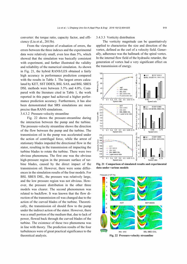
Liu et al. / J Zhejiang Univ-Sci A (Appl Phys & Eng) 2018 19(12):904-925 919
converter: the torque ratio, capacity factor, and effi-ciency (Liu et al., 2015b).
From the viewpoint of evaluation of errors, the errors between the three indexes and the experimental data were relatively small, even less than 5%, which showed that the simulation was basically consistent with experiment, and further illustrated the validity and reliability of the numerical simulation. As shown in Fig. 21, the hybrid RANS/LES obtained a fairly high accuracy in performance prediction compared with the results in Table 1. The largest errors calcu-lated by KET, SST DDES, BSL SAS, and BSL SBES DSL methods were between 3.5% and 4.0%. Com-pared with the literature cited in Table 1, the work reported in this paper had achieved a higher perfor-mance prediction accuracy. Furthermore, it has also been demonstrated that SRS simulations are more precise than RANS simulations. 3.4.3.2 Pressure-velocity streamline
Fig. 22 shows the pressure-streamline during the interaction between the pump and the turbine. The pressure-velocity streamline shows the direction of the flow between the pump and the turbine. The transmission oil in the pump was accelerated under the action of centrifugal force, while the arrest of stationary blades impeded the directional flow in the stator, resulting in the transmission oil impacting the turbine blades to rotate the turbine. There were two obvious phenomena. The first one was the obvious high-pressure region in the pressure surface of tur-bine blades, caused by the direct impact of the transmission oil. However, there were some differ-ences in the simulation results of the four models. For BSL SBES DSL, the pressure was relatively large, and the low pressure region was not obvious. How-ever, the pressure distribution in the other three models was clearer. The second phenomenon was related to backflow. It was known that the flow di-rection of the transmission oil was changed due to the action of the curved blades of the turbine. Theoreti-cally, the transmission oil should flow to the pump under the indirect action of the stator. However, there was a small portion of the medium that, due to lack of power, flowed back through the curved blades of the turbine. The existence of these two phenomena was in line with theory. The prediction results of the four turbulences were of great practical significance to the theoretical analysis.
3.4.3.3 Vorticity distribution The vorticity magnitude can be quantitatively
applied to characterize the size and direction of the vortex, defined as the curl of a velocity field. Gener-ally, adherence was the hallmark of the spiral vortex. In the internal flow field of the hydraulic retarder, the generation of vortex had a very significant effect on the transmission of energy.
Fig. 22 Pressure-velocity streamline
Fig. 21 Comparison of simulated results and experimentaldata under various models

Liu et al. / J Zhejiang Univ-Sci A (Appl Phys & Eng) 2018 19(12):904-925 920
Fig. 23 demonstrates the transient evolutionary process of vorticity on the section. As shown, the vorticity at the blade edges of the pump and the tur-bine was significantly higher than in other regions considered. At the suction surfaces of turbine blades, the vorticity magnitude was slightly higher. Gener-ally, the low pressure region always corresponded to a high vorticity area. Therefore, the flow separation near the suction surfaces of the turbine, resulting from the wake flow of the pump corresponds to the area with low pressure and high vorticity. From the vorti-city as shown in the figure, KET obviously overes-timated the vorticity distribution, while the SST DDES was relatively low in its prediction of vorticity distribution. On balance, the capture ability for the flow structure of hybrid RANS/LES was advanced, especially in the BSL SBES DSL model. 3.4.3.4 Wall shear stress
The fluid near the wall adheres to the wall sur-face because of its viscosity. The viscous effect hin-ders the relative slip between the fluid and the wall, resulting in the generation of wall shear stress. Fig. 24 shows the distribution trend of the wall shear stress on the turbine blade, which represented the energy dis-sipation. The fluid was attached in the near-wall by this stress, and thus energy was consumed. The higher wall shear stress was located in the inlet because of the large velocity gradient, whereas the lower regions were located at one-third of the chord just before the curvature mutation.
3.4.3.5 Quantitative analysis Through the quantitative analysis of pressure
coefficient and skin friction coefficient, as shown in Fig. 25, it can be clearly seen that the energy loss in blade inlet was the maximum. The negative value of Fig. 25 Distributions of pressure coefficient (a) and skinfriction coefficient (b) in blades
Fig. 24 Distribution trend of wall shear stress on turbineblade: (a) pressure surface; (b) suction surface
Fig. 23 Vorticity distribution under the four turbulencemodels
Vorticity (×103 s−1)
Liu et al. / J Zhejiang Univ-Sci A (Appl Phys & Eng) 2018 19(12):904-925 921
pressure coefficient represented the minus differential pressure Δp, which always indicates complicated unsteady flow phenomena. The pressure coefficient was smooth from 0.1 to 0.7, while the pressure loss became larger between 0.7 and 1, which showed that the energy loss in outlet was more serious. Figs. 24 and 25 together indicate that the blade inlet and outlet are the larger flow loss regions, and the inlet espe-cially should be considered in blade design. They prove that SRS simulations can qualitatively and quantitatively analyze the flow loss. 4 Discussion
4.1 Prediction accuracy analysis
SRS simulations are more accurate than RANS modes, mainly because of their capacity for resolving the turbulence spectrum and near-wall treatment with a fine grid. The near-wall treatments consisted of applying wall functions and resolving the viscous sublayer. There is no uniform performance for free shear flows ranging from simple self-similar flows to impinging flows. It is, however, a fact that the RANS models typically only covered the most basic self- similar free shear flows with a set of constants. For that reason, RANS models, even the most advanced Reynolds stress model (RSM), did not have enough capacity to provide a reliable solution for all free shear flows. For free shear flows, LES can resolve large turbulence scales easily, while severe limita-tions for small scale vortex are posed in wall bound-ary layers. Then, hybrid models are developed com-bining the advantages of LES models and RANS models, where large eddies can be resolved by LES models and the wall boundary layers are covered by the RANS models. The hybrid RANS/LES models were very stable and had higher accuracy in the pre-diction of performance.
4.2 Additional information analysis
There are a few simulations that cannot be ex-tracted with accuracy from RANS simulations, such as acoustics simulations and unsteady heat loading. For the turbulent flows in this paper, much important turbulence information was ignored by RANS simu-lations because of the solving method of time average for Reynolds equations, which will have influence on
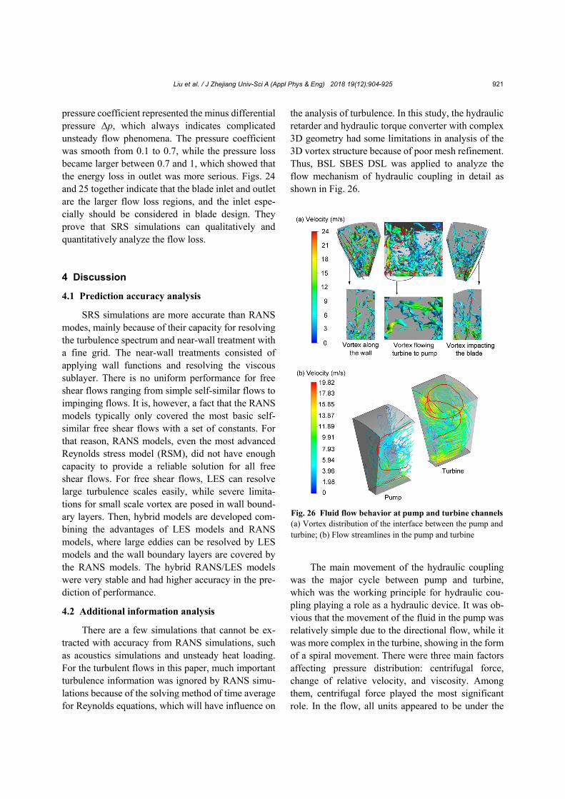
the analysis of turbulence. In this study, the hydraulic retarder and hydraulic torque converter with complex 3D geometry had some limitations in analysis of the 3D vortex structure because of poor mesh refinement. Thus, BSL SBES DSL was applied to analyze the flow mechanism of hydraulic coupling in detail as shown in Fig. 26.
The main movement of the hydraulic coupling was the major cycle between pump and turbine, which was the working principle for hydraulic cou-pling playing a role as a hydraulic device. It was ob-vious that the movement of the fluid in the pump was relatively simple due to the directional flow, while it was more complex in the turbine, showing in the form of a spiral movement. There were three main factors affecting pressure distribution: centrifugal force, change of relative velocity, and viscosity. Among them, centrifugal force played the most significant role. In the flow, all units appeared to be under the
Fig. 26 Fluid flow behavior at pump and turbine channels(a) Vortex distribution of the interface between the pump andturbine; (b) Flow streamlines in the pump and turbine

Liu et al. / J Zhejiang Univ-Sci A (Appl Phys & Eng) 2018 19(12):904-925 922
influence of a centrifugal force proportional to its mass, distance from the axis of rotation, and the square of the angular velocity. It meant that the flow structures behaved differently due to the change of the rotational speed of the pump, for example the position in the interface where the fluid mainly flowed into the turbine varied with the change of speed.
We could also see the movement direction and position of fluid in the field in the figure, which was located between one-third and two-thirds of the blade height. It was a centrifugal movement in the pump for the fluid, and a centripetal movement in the turbine, namely, flowing out at the outer ring and flowing in at the inner ring. The fluid was thrown out along the tangential direction of the outlet surface in the pump as seen in the picture. Due to the pump driving the internal fluid, the fluid was gathered in the central area of the interface with fully developed turbulence (Yan et al., 2009; Li et al., 2012). The vortex structure in the turbine could be seen in the turbine at upper middle and upper left. It was slightly richer at the outer ring, and was very obviously more abundant and complex than that in the pump which was richer at the inner ring. The reason was that the fluid, im-pacting the blade of turbine at a certain speed, flowed into the turbine, developing a turbulent flow. Thus, the fluid, flowing into the pump from the turbine at the inner ring, stirred by the pump developed full turbulence with the energy consumption and velocity change. There was still individual circulation in each channel of the pump and turbine, and a very clear vortex cycle existed in the turbine. It was, therefore, not just a circular movement for the circulation flow between pump and turbine, but a closed spiral movement. The SRS simulation gave the detailed flow structure and was useful in understanding the flow mechanism. 5 Conclusions
In this paper, we focused on CFD applications in hydraulic fluid machineries, such as hydraulic cou-pling, hydraulic retarder, and hydraulic torque con-verter. They employed an incompressible liquid to transfer fluid kinetic energy. SRS approaches, in-cluding LES with various SGS models and hybrid RANS/LES, were employed to improve the predic-
tion of performance and to provide understanding of the flow structures. We assessed them based on al-ready available experimental data and also analyzed the flow field. It was found that those models achieved tasks, which can be shown as follows.
1. Performance prediction. We reviewed the previous RANS simulations and found the prediction errors were mainly 10%–15%. By SRS approaches, the maximum errors were reduced below 10%. Even better results of less than 4% were achieved for the hydraulic coupling and hydraulic torque converter. The results were consistent with the theory that the RANS simulations have limitations in accuracy in certain flow situations.
2. Flow structure description. The improvement of performance prediction was based on capturing the flow field. We conducted many quantitative and qualitative analyses to demonstrate and assess the abilities of those models, involving y+ distribution, pressure-streamline, wall shear stress, pressure coef-ficient, skin friction coefficient, and vortex. The SRS approaches could clearly describe the circulatory motion in hydraulic coupling. The details of fluid transmission between pump and turbine, and flow motion were both demonstrated directly. Hence the flow mechanism in hydraulic coupling was better understood than in previous studies, which inspired and encouraged the researchers in other fluid ma-chineries. For the hydraulic retarder and hydraulic torque converter, although we could not obtain the similar detailed flow structure due to the limitation of computing power in our group, we still captured the unsteady flow field and had a deeper insight into the flow mechanism. In addition, the flow structure demonstrated that the instantaneous flow status of each blade’s passage was not identical, which indi-cated that a simulation based on periodic boundaries of a single blade passage has certain limitations for those devices.
3. Assessment of SRS approaches. It was found that almost all SRS approaches, including LES and hybrid RANS/LES, could obtain reasonable predic-tion results. Therefore, SRS simulation could allevi-ate and avoid the difficulty of choosing appropriate turbulence models as in RANS simulation. Compared with LES model, the hybrid RANS/LES model was more computationally efficient, as shown by the performance prediction. A new developed hybrid

Liu et al. / J Zhejiang Univ-Sci A (Appl Phys & Eng) 2018 19(12):904-925 923
RANS/LES method was preferred for use because of its good prediction accuracy, flow structure descrip-tion, and computational cost. The suggestion based on the work in this study was that, for unsteady flow field simulations of hydrokinetic devices, the BSL SBES DSL model safely achieved good results, and is strongly recommended.
Our work primarily verified that SRS ap-proaches were advanced and practical in hydrokinetic devices. Many further studies should be carried out. The simulations used commercial code, so the ap-proaches can be developed and adapted. The com-putational setup and grid should also be well inves-tigated to give full play to the advantages of SRS approaches. During simulation, the density and vis-cosity of the working medium should be considered fully. The calculation of two-phase flow and bound-ary layer flow also needs to be elaborated. Further-more, it was necessary to employ volume of fluid to track gas-liquid distribution within the passage of hydraulic retarder for improving its performance. The grid employed in this study will be improved, espe-cially in the hydraulic torque converter and hydraulic retarder, to eventually capture the flow motion during fluid kinetic energy transmission.
References Andersson S, 1986. Analysis of multi-element torque con-
verter transmissions. International Journal of Mechanical Sciences, 28(7):431-441. https://doi.org/10.1016/0020-7403(86)90063-9
Bai L, Fiebig M, Mitra NK, 1997. Numerical analysis of tur-bulent flow in fluid couplings. Journal of Fluids Engi-neering, 119(3):569-576. https://doi.org/10.1115/1.2819282
Denton JD, 1986. The use of a distributed body force to sim-ulate viscous effects in 3D flow calculations. Proceedings of ASME 1986 International Gas Turbine Conference and Exhibit, p.V001T01A058. https://doi.org/10.1115/86-GT-144
Denton JD, 2010. Some limitations of turbomachinery CFD. Proceedings of ASME Turbo Expo 2010: Power for Land, Sea, and Air, p.735-745. https://doi.org/10.1115/GT2010-22540
Duchaine F, Maheu N, Moureau V, et al., 2013. Large-eddy simulation and conjugate heat transfer around a low-Mach turbine blade. Proceedings of ASME Turbo Expo 2013: Turbine Technical Conference and Exposi-tion, p.V03BT11A004. https://doi.org/10.1115/GT2013-94257
Ejiri E, Kubo M, 1999. Influence of the flatness ratio of an automotive torque converter on hydrodynamic perfor-
mance. Journal of Fluids Engineering, 121(3):614-620. https://doi.org/10.1115/1.2823513
Flack R, Brun K, 2003. Fundamental analysis of the secondary flows and jet-wake in a torque converter pump: part 2— flow in a curved stationary passage and combined flows. ASME/JSME 2003 4th Joint Fluids Summer Engineering Conference, p.1193-1201. https://doi.org/10.1115/FEDSM2003-45402
Gourdain N, Sicot F, Duchaine F, et al., 2014. Large eddy simulation of flows in industrial compressors: a path from 2015 to 2035. Philosophical Transactions of the Royal Society A: Mathematical, Physical and Engineering Sci-ences, 372(2022):20130323. https://doi.org/10.1098/rsta.2013.0323
Gritskevich MS, Garbaruk AV, Menter FR, 2014. Computa-tion of wall bounded flows with heat transfer in the framework of SRS approaches. Journal of Physics: Conference Series, 572(1):012057. https://doi.org/10.1088/1742-6596/572/1/012057
Hampel U, Hoppe D, Diele KH, et al., 2005. Application of gamma tomography to the measurement of fluid distri-butions in a hydrodynamic coupling. Flow Measurement and Instrumentation, 16(2-3):85-90. https://doi.org/10.1016/j.flowmeasinst.2004.10.001
He YD, Ma WX, Liu CB, 2009a. Numerical simulation on CFD of flow field in hydrodynamic coupling and char-acteristics prediction. Proceedings of Asia-Pacific Power and Energy Engineering Conference, p.1-4. https://doi.org/10.1109/APPEEC.2009.4918546
He YD, Ma WX, Liu CB, 2009b. Numerical simulation and characteristic calculation of hydrodynamic coupling. Transactions of the Chinese Society for Agricultural Machinery, 40(5):24-28 (in Chinese).
Hedman A, 1992. Analysis of transmissions with multi-turbine hydrodynamic torque converters. Mechanism and Ma-chine Theory, 27(5):543-554. https://doi.org/10.1016/0094-114X(92)90043-H
Hu DF, Huang ZL, Sun JY, et al., 2017. Numerical simulation of gas-liquid flow through a 90° duct bend with a gradual contraction pipe. Journal of Zhejiang University- SCIENCE A (Applied Physics & Engineering), 18(5): 212-224. https://doi.org/10.1631/jzus.A1600016
Huang JG, Li CY, 2013. Whole-flow-passage numerical sim-ulation and experimental validation on idling loss of hy-drodynamic retarder. Transactions of the Chinese Society of Agricultural Engineering, 29(24):56-62 (in Chinese). https://doi.org/10.3969/j.issn.1002-6819.2013.24.008
Huitenga H, Mitra NK, 2000a. Improving startup behavior of fluid couplings through modification of runner geometry: part I–fluid flow analysis and proposed improvement. Journal of Fluids Engineering, 122(4):683-688. https://doi.org/10.1115/1.1319501
Huitenga H, Mitra NK, 2000b. Improving startup behavior of fluid couplings through modification of runner geometry: part II–modification of runner geometry and its effects on

Liu et al. / J Zhejiang Univ-Sci A (Appl Phys & Eng) 2018 19(12):904-925 924
the operation characteristics. Journal of Fluids Engi-neering, 122(4):689-693. https://doi.org/10.1115/1.1319502
Ji SM, Ge JQ, Tan DP, 2017. Wall contact effects of particle- wall collision process in a two-phase particle fluid. Journal of Zhejiang University-SCIENCE A (Applied Physics & Engineering), 18(3):958-973. https://doi.org/10.1631/jzus.A1700039
Johnston JP, 1998. Effects of system rotation on turbulence structure: a review relevant to turbomachinery flows. In-ternational Journal of Rotating Machinery, 4(2):97-112. https://doi.org/10.1155/S1023621X98000098
Jung JH, Kang S, Hur N, 2011. A numerical study of a torque converter with various methods for the accuracy im-provement of performance prediction. Progress in Computational Fluid Dynamics, An International Jour-nal, 11(3-4):261-268. https://doi.org/10.1504/PCFD.2011.041027
Kim BS, Ha SB, Lim WS, et al., 2008. Performance estimation model of a torque converter part I: correlation between the internal flow field and energy loss coefficient. Inter-national Journal of Automotive Technology, 9(2):141- 148. https://doi.org/10.1007/s12239-008-0018-5
Lakshminarayana B, 1991. An assessment of computational fluid dynamic techniques in the analysis and design of turbomachinery—the 1990 freeman scholar lecture. Journal of Fluids Engineering, 113(3):315-352. https://doi.org/10.1115/1.2909503
Lee C, Jang W, Lee JM, et al., 2000. Three Dimensional Flow Field Simulation to Estimate Performance of a Torque Converter. SAE Technical Paper 2000-01-1146, SAE International. https://doi.org/10.4271/2000-01-1146
Lei YL, Wang C, Liu ZJ, et al., 2012. Analysis of the full flow field of torque converter. Advanced Materials Research, 468-471:674-677. https://doi.org/10.4028/www.scientific.net/amr.468-471.674
Li XS, Yu XM, Cheng XS, et al., 2012. Large eddy simulation and characteristic prediction of transient two-phase flow for hydraulic retarder. Journal of Jiangsu University (Natural Science Edition), 33(4):385-389 (in Chinese). https://doi.org/10.3969/j.issn.1671-7775.2012.04.003
Liu CB, Ma WX, Zhu XL, 2010. 3D transient calculation of internal flow field for hydrodynamic torque converter. Journal of Mechanical Engineering, 46(14):161-166 (in Chinese). https://doi.org/10.3901/JME.2010.14.161
Liu CB, Xu D, Ma WX, et al., 2015a. Analysis of unsteady rotor-stator flow with variable viscosity based on ex-periments and CFD simulations. Numerical Heat Trans-fer, Part A: Applications, 68(12):1351-1368. https://doi.org/10.1080/10407782.2015.1052298
Liu CB, Liu CS, Ma WX, 2015b. RANS, detached eddy sim-ulation and large eddy simulation of internal torque converters flows: a comparative study. Engineering Ap-
plications of Computational Fluid Mechanics, 9(1):114- 125. https://doi.org/10.1080/19942060.2015.1004814
Liu Y, Pan YX, Liu CB, 2007. Numerical analysis on three-dimensional flow field of turbine in torque con-verter. Chinese Journal of Mechanical Engineering, 20(2):94-96.
Menzies K, 2009. Large eddy simulation applications in gas turbines. Philosophical Transactions of the Royal Society A: Mathematical, Physical and Engineering Sciences, 367(1899):2827-2838. https://doi.org/10.1098/rsta.2009.0064
Park JI, Cho KR, 1998. Numerical flow analysis of torque converter using interrow mixing model. JSME Interna-tional Journal Series B, 41(4):847-854. https://doi.org/10.1299/jsmeb.41.847
Schulz H, Greim R, Volgmann W, 1996. Calculation of three-dimensional viscous flow in hydrodynamic torque converters. Journal of Turbomachinery, 118(3):578-589. https://doi.org/10.1115/1.2836705
Shieh T, Perng C, Chu D, et al., 2000. Torque Converter An-alytical Program for Blade Design Process. SAE Tech-nical Paper 2000-01-1145, SAE International. https://doi.org/10.4271/2000-01-1145
Shin S, Chang H, Athavale M, 1999. Numerical Investigation of the Pump Flow in an Automotive Torque Converter. SAE Technical Paper 1999-01-1056, SAE International. https://doi.org/10.4271/1999-01-1056
Song B, Lü JG, Guo SY, et al., 2011. Simulation and charac-teristic analysis on flow field of fluid couplings during braking. Machine Design and Research, 27(1):26-30 (in Chinese).
Sun Z, Chew J, Fomison N, et al., 2009. Analysis of fluid flow and heat transfer in industrial fluid couplings. Proceed-ings of the Institution of Mechanical Engineers, Part C: Journal of Mechanical Engineering Science, 223(9): 2049-2062. https://doi.org/10.1243/09544062JMES1478
Tucker P, Eastwood S, Klostermeier C, et al., 2012a. Hybrid LES approach for practical turbomachinery flows–part I: hierarchy and example simulations. Journal of Tur-bomachinery, 134(2):021023. https://doi.org/10.1115/1.4003061
Tucker P, Eastwood S, Klostermeier C, et al., 2012b. Hybrid LES approach for practical turbomachinery flows–part II: further applications. Journal of Turbomachinery, 134(2): 021024. https://doi.org/10.1115/1.4003062
Tucker PG, 2011a. Computation of unsteady turbomachinery flows: part 1—progress and challenges. Progress in Aerospace Sciences, 47(7):522-545. https://doi.org/10.1016/j.paerosci.2011.06.004
Tucker PG, 2011b. Computation of unsteady turbomachinery flows: part 2—LES and hybrids. Progress in Aerospace Sciences, 47(7):546-569. https://doi.org/10.1016/j.paerosci.2011.07.002

Liu et al. / J Zhejiang Univ-Sci A (Appl Phys & Eng) 2018 19(12):904-925 925
Tucker PG, 2013. Trends in turbomachinery turbulence treatments. Progress in Aerospace Sciences, 63(6):1-32. https://doi.org/10.1016/j.paerosci.2013.06.001
Tyacke J, Tucker P, Jefferson-Loveday R, et al., 2014. Large eddy simulation for turbines: methodologies, cost and future outlooks. Journal of Turbomachinery, 136(6): 061009. https://doi.org/10.1115/1.4025589
Wang XB, Liu Y, Cui HQ, et al., 2012. Experimental study on the fluid flow characteristics in the hydrocyclone on the PIV. Fluid Machinery, 40(2):5-9 (in Chinese). https://doi.org/10.3969/j.issn.1005-0329.2012.02.002
Whitfield A, Wallace FJ, Sivalingam R, 1978. A performance prediction procedure for three element torque converters. International Journal of Mechanical Sciences, 20(12): 801-814. https://doi.org/10.1016/0020-7403(78)90006-1
Wu GQ, Yan P, 2008. System for torque converter design and analysis based on CAD/CFD integrated platform. Chinese Journal of Mechanical Engineering, 21(4):35-39. https://doi.org/10.3901/CJME.2008.04.035
Wu GQ, Wang LJ, 2015. Multi-objective Optimization em-ploying genetic algorithm for the torque converter with dual-blade stator. SAE Technical Paper 2015-01-1119, SAE International. https://doi.org/10.4271/2015-01-1119
Wu HX, Tan D, Miorini RL, et al., 2011. Three-dimensional flow structures and associated turbulence in the tip region of a waterjet pump rotor blade. Experiments in Fluids, 51(6):1721-1737. https://doi.org/10.1007/s00348-011-1189-9
Yan J, He R, Lu M, 2009. Numerical simulation of hydraulic retarder with different blade number. Journal of Jiangsu University (Natural Science Edition), 30(1):27-31 (in Chinese).
Yang ZY, 2015. Large-eddy simulation: past, present and the future. Chinese Journal of Aeronautics, 28(1):11-24. https://doi.org/10.1016/j.cja.2014.12.007
Zhang TT, Huang W, Wang ZG, et al., 2016. A study of airfoil parameterization, modeling, and optimization based on the computational fluid dynamics method. Journal of Zhejiang University-SCIENCE A (Applied Physics & Engineering), 17(3):632-645. https://doi.org/10.1631/jzus.A1500308
中文概要
题 目:尺度解析模拟在液力偶合器、液力缓速器和液力
变矩器中的应用
目 的:针对流体机械数值模拟过程中雷诺时均应力
(RANS)方法占据主导地位但预测精度较低且
缺乏对流场信息准确描述的现状,提出应用尺度
解析模拟(SRS)方法来改进性能的预测精度以
及加深对流动结构的理解。
创新点:1. 利用 SRS 方法,降低 RANS 湍流模型的选择困
难,实现性能精准预测;2. 建立全流道网格计算
模型,充分展现单流道间瞬时流动信息的差异。
方 法:1. 通过较少的网格划分及周期计算,对具有简单
循环圆和平面叶片的液力偶合器进行计算,并与
试验数据进行对比,初步筛选出较为适合的湍流
模型(图 6),进而在模型更为复杂、流动更加多
变的液力缓速器和液力变矩器性能预测中进行
验证(图 15 和 21);2. 通过对复杂的瞬态流动现
象的清晰捕捉,深入展示 3 种液力元件的内部流
动机理(图 9、10、16、17、22 和 23),并评估
SRS方法相较RANS方法在流动结构描述方面的
先进性(图 7 和 8)。
结 论:1. 在液力偶合器、液力缓速器和液力变矩器等液
力流体机械的计算流体动力学(CFD)模拟中,
SRS方法可以提高性能预测精度并提供更为细致
的流场信息;2. SRS 方法中的混合 RANS/LES(大
涡模拟)模型在液力元件流场计算中的预测准确
度、流场结构描述及计算成本等方面表现出色,
尤其是 BSL SBES DSL 模型值得重点关注和发
展;3. 为了进一步验证 SRS 方法的实用性,可以
在模拟中考虑工作介质物理属性的影响,细化网
格并对气液两相流动及边界层流动进行详细计
算。
关键词:尺度解析模拟;混合 RANS/LES;液力偶合器;
液力缓速器;液力变矩器