Application of Malliavin calculus to a class of stochastic differential equations

Probab. Th. Rel. Fields 84, 549-571 (1990) Probability Theory M, Related Fields

�9 Springer-Verlag 1990

Application of Malliavin Calculus to a Class of Stochastic Differential Equations

Nguyen Minh Duc 1'*, D. Nualar t 2'**, and M. Sanz 2'**

1 Institute of Computer Science and Cybernetics, Nghia Do-Tu Liem, Hanoi, R.S. Vietnam 2 Facultat de Matem/ttiques, Universitat de Barcelona, Gran Via 585, E-08007 Barcelona, Spain

Summary. In this article we deal with stochastic differential equations driven by an infinite dimensional Brownian motion. Under some non-degeneracy conditions, the existence and smoothness of the density for the law of the solution is proved.

Introduction

In this paper we study the existence and smoothness of the density for the law of the d-dimensional random vector Xt(t > O) given by the stochastic differential system

k = l 0 0

Here x o ~ IR d, {B k, t ~ [0, 1], k > 1} is a sequence of independent standard Brownian motions, and the coefficients are given by a map F: IRd-*IRe | N, F={F~, k > 1, P ~ ; i = 1 .. . . . d} satisfying some Lipschitz condition. Our aim is to prove a version of HSrmander ' s theorem in this situation.

Equation (0.1) can be viewed as a particular case of stochastic integral equations driven by nonlinear integrators. That means, equations of the type

t

x, =Xo +~ z(x~, ds), (0.2) 0

where Z(x, t) is a d-dimensional semimartingale depending on the parameter x e IR d. The integral in (0.2) is a nonlinear stochastic integral. It is defined in such a way that if Z(x, t)=xZt, then it coincides with the usual I t6 's integral. We refer the reader to [12, 5, 4] and finally to [2] for an extensive treatment of this subject.

* The work of Nguyen Minh Duc was done during a stay at the University of Barcelona (Spain) ** The work of D. Nualart and M. Sanz has been supported by the Grant of the C.Y.C.I.T. number PB86-0238

550 M.D. Nguyen et al.

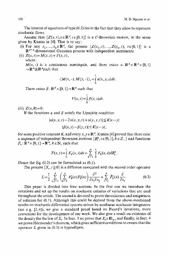
The interest of equations of type (0.2) lies in the fact that they allow to represent stochastic flows.

Assume that {Z(x, t),xeiR d, te [0, 1]} is a C-Brownian motion, in the sense given by Kunita in [4]. That is to say:

(i) For any x~ ..... x ,~ iR e, the process {Z(xl,t) , . . . ,Z(x,, t) , te[0,1]} is a IR e • Gaussian process with independent increments.

(ii) Z(x, t)=M(x, t)+ V(x, t), where: M(x, .) is a continuous martingale, and there exists c~:iRdx~'..ex [0, 1] ~iRe| that

t (M(x, .), M(y, "))t = I e(x, y, s)ds.

0

There exists/~ : IR a x [0, 1]~IR e such that

t V(x, 0 B(x, s)ds.

0

(iii) Z(x, 0) = 0 . If the functions c~ and/~ satisfy the Lipschitz condition

I~(x, x, t) - 2 c~(x, y, t) + ~(y, y, t)l < Klx-y[

[/~(x, t) - /~(y, t)l < KIx-yl ,

for some positive constant K, and every x, y e IRe Kunita [4] proved that there exist a sequence of independent Brownian motions {B~, t ~ [0, 1 ], k e Z+ } and functions Fk : ] R e • [0, I]---~IR d, k e N , such that

0 k= l 0

Hence the Eq. (0.2) can be formulated as (0.1). The process {Xt, t > 0} is a diffusion associated with the second order operator

1 i ~ (0 .3)

This paper is divided into four sections. In the first one we introduce the notations and set up the results on stochastic calculus of variations that are used throughout the article. The second is devoted to prove the existence and uniqueness of solution for (0.1). Although this could be derived from the above-mentioned results on stochastic differential systems driven by nonlinear stochastic integrators (see e.g. [2,4]), we give a standard proof based on Picard's iterations, more convenient for the development of our work. We also give a result on existence of the density for the law ofXt. In Sect. 3 we prove that X t e ~)~, and finally, in Sect. 4 we prove H6rmander 's theorem, which gives sufficient conditions to ensure that the operator L given in (0.3) is hypoelliptic.

Application of Malliavin Calculus to a Class of S.D.E. 551

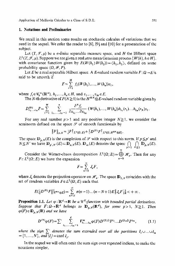
1. Notations and Preliminaries

We recall in this section some results on stochastic calculus of variations that we need in the sequel. We refer the reader to [8], [9] and [10] for a presentation of the subject.

Let (T, 3--,/~) be a a-finite separable measure space, and H the Hilbert space L 2 (T, ~-, p). Suppose we are given a real zero mean Gaussian process { W(h), h ~ I-I}, with covariance function given by E(W(hl)W(h2))=<hl , ha), defined on some probability space (0, ~ , P ).

Let E be a real separable Hilbert space. A E-valued random variable F: ~ E is said to be smooth if

M

F= ~ f i (W(hO, . . . , W(h,))v,, i=1

where f i e c ~ ( l R ' ) , h 1 .. . . . hnEH , and v 1 .... ,vMEE. The N-th derivative o f F ( N > 1) is the H | | random variable given by

M ~ ~Nf~ D(N)rx...,NF-- i=a • i,,...,i~,=x Oxii:~.Oxi,, (W(h l ) ' " " W(h"))hi~(rl)"'hi~'(rNlVi"

For any real number p > l and any positive integer N__>I, we consider the seminorm defined on the space 5 r of smooth functionals by

I[V[Ip, N = []FIIL"(O;E)+ liD (u'F[IL,(o;H|174 .

The space K)p, N ( E ) is the completion of 6 p with respect to this norm. Ifp__<p' and N_~N' we have Dp,,N,(E)cDp, N(E ). lDoo(E ) denotes the space /") (~ IDp, N(E ).

p > l N>=I C / 5

Consider the Wiener-chaos decomposition L2(O; E)= ~) ~t~ Then for any F~L2(O;E) we have the expansion ,=o

F = ~ J , r , n=O

where J, denotes the projection operator on W.. The space Da, N coincides with the set of random variables F~ L 2 (Q; E) such that

E(IIDtN)FIIZn*~| ~ n(n- -1 ) . . . (n - -N+ l)EllJ.FII2 < + o o . n = N

Proposition 1.1. Let ~o : lR d ~ be a cgU-funetion with bounded partial derivatives. Suppose that F : O - ~ R a belongs to IDp, N(IRa), for some p > l , N > I . Then q~(F) e ID v, N(IR ) and we have

d

D(N)q~(F)=~ ' ~ V. m �9 ,o(F~Dtlhl)F h D(I/'~I)F ~" (1.1) i a , - . . , i m = l

where the sign ~ ' denotes the sum extended over all the partitions I t w . . . u I m = {1 ..... , N}, and IIjl =ca rd l j .

In the sequel we will often omit the sum sign over repeated indices, to make the notations simpler.


The proof of (1.1) follows easily by approximating F by smooth functionals. By 6 (s) we denote the dual of the operator D (m defined o n L2(O • TN; E). The

domain of c5 (N), denoted by Dora 6 (m (E), is the set of processes u ~ L 2 (~ • T N; E) = L 2 ( ~ ; H|174 such that there exists a constant C with

[E( (u, D~m F) ~|174 <= C f]FI[L2(O;E~, for any FeSP.

Then, if F~ D2,N(E), and u e Dom 6r we have the duality relation

E ( (u, D(N) F) H,N| = E( ( fCm(u), F)~) . (1.2)

We point out that 6 (N) coincides with the multiple Ramer-Skorohod integral (see [9]).

The next result shows how to compute the N-th derivative ofa Ramer-Skorohod integral.

Proposition 1.2. Let u~)Z,N(H@E ) be such that D~U)r, ...~,~ u belongs to Dom 6(E), VM<N, for any (r~ . . . . . rM), l~M--a.e., and suppose that ~ g(l~(O~,~!.,,,u)l z)

T M

# (dr 1)... # (dr M) < oe, for any M <= N. Then 6 (u) ~ I1)2, N (E) and

N

O~m .,~,(6 (u)) ----(N) (1.3) =0tL ' ... . . . ~,U)+ ~ D (N-~) l ' l �9 , r l , . , r v - I P r I - �9 , r N U r ~ "

Proof. For N = 1, this is Proposition 3.3 of [10]. Assume that the assertion is true for N - l , i.e.

N - - 1

( N - I ) _ " D ( N - ~ ) D N - 2 r, . . . . Z . . . . . .

e = l

Then, using formula (1.3) for N = 1 we have

N - 1

D,(N. ) . . . . (6 (u)) = 6 (DCf.)..,N u) + D})~.7.1,)~_, u,~ + E D (s-l) ?1 . , , r ~ - 1 }'~+ 1 . �9 . I ' N - l r l V U I ' ~ "

e = l

Hence the proposition is proved. []

In this article we will use the above mentioned results in the following situation. T= [0, 1] x Z+, endowed with the product measure # = 2 x v, where 2 denotes the Lebesgue measure and v the counting measure. The Hilbert space H is the set of

functions h ' [0 , 1]--,IR z§ such that i ~ Ihk (s)12ds< + go with the inner product 0 k = l

-i (h, h' ) ,u- ~ (hk(s)h/,(s))ds. For any h e H, the Gaussian random variable W(h) 0 k = l

is given by 1

W(h) = ~ ~ hk(s)dB~, k = l 0

where {Bk, s~[O, 1],k~Z+} is a sequence of independent standard Brownian motions. The Hilbert space E will be IR d. I f F ~ IDp, N (IR d) the N-th derivative D(mF is the process /~,~...~rntmJ~"'J"F, (s t .... ,SN)E [0, 1] N, (Jl, .... jN) eZU+}. I t c a n also be viewed as a random variable taking values on [0, 1]Nx Z+ N x IR d such that

A p p l i c a t i o n o f M a l l i a v i n C a l c u l u s to a C l a s s o f S. D . E, 553

~ S l . �9 .SN x t~o 1 [0,1] N j l . . . . . j N = I i = 1

Last remarks. We will not distinguish between constants. All of them will be denoted by C, although they are not necessarily the same. From now on T will denote the time parameter space [0, 1].

2. Existence and Some Properties of the Solution

B k Let { , , tE T , k > l } be a sequence of independent standard Brownian motions. We consider on the space of matrices IRd| N the norm given by

/ / d m x~1/2

I [x l l= [2 2 Ix}12/ �9 Assume we are given a map F'IRe-~IRe| N, \ i = 1 j = o /

F= {F k, k > 1, Po} satisfying the Lipschitz condition

(L) [IF(x)-F(y)[I <-K[x-yl, for any x, yeiRa.

Consider the stochastic differential equation

X~=xo+ ~ i Fk(Xs)dBk+i Fo(Xs)ds, (2.1) k = l 0 0

where Xo~iR a, and t~[0, 1]. The Eq. (2.1) is well-defined for processes Xbelonging to L=(O • T; IRa), due to

property (L). Our first purpose is to prove the existence and uniqueness of solution for (2.1).

Theorem 2.1. Assume that condition (L) is satisfied. Then there exists a unique stochastic process {Xt, t~ T) which satisfies (2.1). Moreover, {Xt, t6 T} has a.s.

f paths, and E{ sup IXtIP~< +oo,for any p>2. continuous

~.o<t<l J

Proof. We can construct the solution as the limit of Picard's iterations. Indeed, we define Xt(0 ) = Xo,

t

Xt(n+l)=xo+ ~ i Fk(X~(n))dBk+~ Fo(Xs(n)) ds, for n>__0. (2.2) k = l 0 0

We first prove, by induction on n, that for anyp _> 2, E (sup IX,(n)[@ < + ~ , so that - - ~ t ~ T ]

(2.2) makes sense. In fact, Burkholder's and H61der's inequalities imply

E~sup[Xt(n+l)lV}.<C{lxof+E(! ~ ,p12 l 'Fk(Xs(n))[2ds)+E}[Fo(Xs(n)l l 'ds} ~teT k = l ' 0

<C,+C2E{sup,Xt(n)IP}. (2.3)

554 M . D . N g u y e n et al.

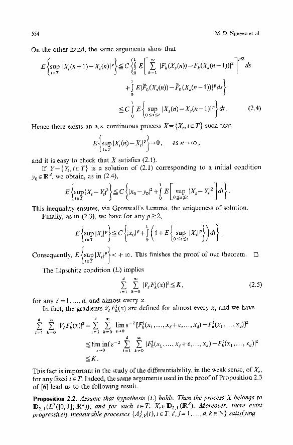
On the other hand, the same arguments show that

E t s u p [Xt(n+l)-Xt(n)[P}<-C{iEIk~__ ~ [Fk(Xs(n))--Fk(Xs(n-1))[2] p/2 _ ds ~t~T

+S ElPo(X~(n))-Po(X~(n- O)l~ds 0

0 [0_<s-<t

Hence there exists an a.s. continuous process X = {X t, t e T} such that

E tsuplX,(n)-Xt, v}~O, as n-~oo, ~ t s r

and it is easy to check that X satisfies (2.1). If Y={Yt, t eT} is a solution of (2.1) corresponding to a initial condition

Yo e IR d, we obtain, as in (2.4),

This inequality ensures, via Gronwall's Lemma, the uniqueness of solution. Finally, as in (2.3), we have for any p >2,

E(suplXt[Pt<--C{lxolP+i(I+E~sup [X~[P})dt} �9 ( t~T . )-- [O<-s<-t

E~sup IX, lP~< + o0. This finishes the proof of our theorem. [] Consequently, ~t~T )

The Lipschitz condition (L) implies d

Z ~ IVeF~(x)[ 2NK, (2.5) i=1 k = 0

for any Y = 1 ..... d, and almost every x. In fact, the gradients VeF~(x) are defined for almost every x, and we have

d

i=1 k = 0

= - F f ( x l . . . . , x d ) ] 2 [VeF~(x)[ 2 ~, lim ~-2 [~s .... ,xe+e ..... xe) ; i = i k = 0 e--*0

=<lim infe -2 ~ [F~(x t .... , xe+e .... , xa) -F~(xl ..... xd)[ z e--~O i=1 k = 0

< K .

This fact is important in the study of the differentiability, in the weak sense, of Xt, for any fixed t ~ T. Indeed, the same arguments used in the proof of Proposition 2.3 of [6] lead us to the following result.

Proposition 2.2. Assume that hypothesis (L) holds. Then the process X belongs to D2,1(LZ([O, 1];IRa)), and for each teT, XteD2,~(lRa). Moreover, there exist progressively measurable processes {A], k (t), t e T, E, j = 1 ..... d, k ~ N} satisfying


d

sup Z ~ IA],k(t)] z<K, (2.6) t e T j,~-I k = 0

for any E = 1,..., d, such that the derivath~e of Xt is the solution of the stochastic differential system

rx~ t

, Ae, o(s)D,X~ds, i f r<t k = l r r

i j D,X~ = 0 , / j ' r > t ,

with i >= l, and j = l ..... d.

Remark. If the coefficients Fk, k ~ l and ~'o are cg~-functions, then the processes A],k(s) coincide with VtF~(Z~), for k > l , and A},o(S)= VeP~(X~).

Consider the process { Y] (t, r), t > r, (r, t)~ T2;j, Y = 1 ..... d} solution of

Y](t,r)=6]+ ~ i A~,~(s)yeh(s,r)dB:+i AJh,o(s)Ye%~,r) dy. (2.7) k = l r r

Due to (2,6)such a process exists and satisfies E~ sup Iu +~ , for any (o_<s_<l

p >= 2. Moreover, each component Y~(t, r) has a version a. s. continuous in r for any fixed t. Indeed, we have for r_< r' _< t

E[ 'YJ(t'r)-YJ(t'r')'41<=l'+I2+I3+l"

with

21 = e ALk(s) ~ ( s , r laB ~, , k=l r

I 2 - e Z ~,o(S)V(s,r)ds , U=I r

h---e A~,~(s)(V(s, r ) - V(s, r'))dB~ , j r '

I4--E ~=1 AJh'~ V(s'r'))ds " .i

Let us analyze each one of these terms. By Burkholder's and H61der's inequalities

II <=CE Z ]AJh,~ (s)Yeh(s,r)lz \ j = l k = l

< c g sup ]A~,k(s)l ~ IYeh(s,r)l'ds \ j = l h = l r h k = l

<-CK2E~(o~s~lsup IY~(s,r)J4}lr'-rl2<=Clr'-r] 2.

Analogously, I z <_ Clr'-r[ 2.

556 M, D. Nguyen et al.

On the other hand

t i <cE y. V(s,r')l ds L j = l k = l

<=CE Y. sup rA/.k(s)l 2 I V ( s , r ) - V(s,r')l 2 ds ds [ . j = l 0 h k = l h= l

<-_CK 2 E [Yeh(s,r)-- ~h(s,r')l 4 ds, 0 h

and the same bound holds for I 2. Consequently, by Gronwall 's Lemma we obtain

E[I Yj(t, r) - Y/(t, r')l 4] =< C l r ' - r l 2 ,

and Kolmogorov 's continuity criterium allow us to conclude. We notice that D~,X] = F((Xr) ~ ( t , r). Therefore the process {D~X/, 0 < r < t}, for

any fixed i> 1, j = 1 ... . . d and t~ T possess an a.s.-continuous version. The next result provides a sufficient condition for the existence of a density for

the law of Xt.

Proposition 2.3. Assume that condition (L) holds and that the vector space generated by the vector fields F 1 (x), F 2 (x) .... has dimension d, for any x ~ IR d. Then,for any t > O, the law o f X t has a density.

Proof By the results of Bouleau and Hirsch (see [1]) it suffices to prove that det F( t ) > 0 a.s. where

F( t ) = ( ( D X ] , DXtt >H,j, #= 1 . . . . . d) .

Let A={co, de tF ( t )= O} , and assume that P ( A ) > 0 . Then, if co~A, there exists v ~ IR n, [v[ = 1, such that v*F(t )v =0. That means

0 k = l j = l

d

Consequently, for any k__>l and r~[0, t], ~ D,kX~vj=O. In particular j = l

d

F~(Xt)vj=O, for any k > l , and this leads to a contradiction. [] j = l

3. Differentiability of the Solution

The purpose of this section is to prove that, for any t E T, the random vector X t belongs to the space D~(IRd). To accomplish our aim we need much more regularity on the coefficients of (2.1) than in the preceding section. More precisely we need the following condition

(B) For any multi-index (nl . . . . . n j) with n = n 1 +. . . + n j, n >->_ 1,

Application of Malliavin Calculus to a Class of S. D.E. 557

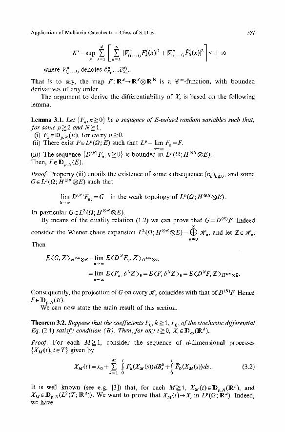
1 K' = sup . i 2 n - i 2 IVil...ifl,(x)[ +ll7,,...,f~(x)l +oo x i = 1 k = l

where ViT...ij denotes 3x~... ~{.

That is to say, the map F:IRa~IRd| N is a cg~~ with bounded derivatives of any order.

The argument to derive the differentiability of X z is based on the following lemma.

Lemma 3.1. Let {F,, n >0} be a sequence of E-valued random variables such that, for some p >2 and N> I,

(i) F,~Dv, N(E), for every n>0. (ii) There exist F~LP(f2; E) such that L v - lira F , = F .

n---~ tx3

(iii) The sequence {D~N)Fn, n >0} is bounded in LP(f2; H|174 Then, F~ Dv, N(E).

Proof. Property (iii) entails the existence of some subsequence (nk)k>=0, and some G ~ LV(O; H | | such that

lira D~mF, k= G in the weak topology of LP(f2; H|174 k - * o 0

In particular G~LZ(Y2; H|174 By means of the duality relation (1.2) we can prove that G=D(N)F. Indeed

consider the Wiener-chaos expansion L2(O; H|174 ~ ~ff,, and let Z~ ovg n. n = 0

Then

E(G, Z)H~| tim E(DNF., Z)H~| n ~ o o

= lim E(F., 6NZ)e=E(F, 6NZ)~ =E(DNF, Z)H~"| n . . ~ oo

Consequently, the projection of G on every ~'~, coincides with that of D(N)F. Hence F~ Dp, N (E).

We can now state the main result of this section.

Theorem 3.2. Suppose that the coefficients Fk, k > 1, Fo, of the stochastic differential Eq. (2.1) satisfy condition ( B ) . Then, for any t>0 , Xt 6 lD oo (IR d).

Proof For each M > I , consider the sequence of d-dimensional processes {XM(t), t~ T} given by

M t t

XM(t)=Xo+ ~ S Fk(XM(s))dB~ + S Fo(XM(S)) ds" (3.2) k = l 0 0

It is well known (see e.g. [3]) that, for each M > I , XM(t)eDV, N(IRd), and XM~Dp, N(L2(T; IRd)). We want to prove that XM(t)~X t in LV(O; IRa). Indeed, we have


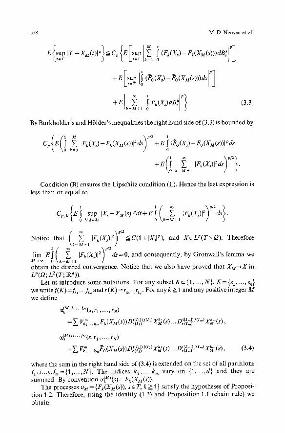
E stup[Xt-Xu(t)[P <=C, E sup 2 i(Fk(X,)--Fk(XM(S)))de: k kt~r Ik=l 0

Fk(X,)dB, . (3.3) + E k= +1 0

By Burkholder's and H61der's inequalities the right hand side of (3.3) is bounded by

{ ( i 1

Condition (B) ensures the Lipschitz condition (L). Hence the last expression is less than or equal to

f 1 Cp, r E ~ sup 00<-s<-t

iXs_ XM(S)[Pdt + E i (k=~+ a \ p/2 o

Notice that (k=M+l ~ IFk(Xs)[2t p/2~C(J-t-IXsIp)~ and X~LP(Txf2). Therefore

l i m E i ( ~, IFk(Xs)12)P/2ds=O, andconsequently, byGronwall 'slemmawe M~oo 0 k=M+l obtain the desired convergence. Notice that we also have proved that XM-*X in LP(Q; L2(T; IRa)).

Let us introduce some notations. For any subset K c {1 ..... N}, K = {e 1 ... . . %} we writej(K) =j,~...j~, and r(K) = r, .... r~. For any k_>_ 1 and any positive integer M we define

r l . . . . .

m Ig ( Y (~X~l ' l ( l l l l ) j ( I1)ykxl 'o~ I '~(lI~l)J(Im)~kmgc~ ---~'2 Vkl...km" kk '~ tMl '~ "eXMk~ . . . . r(Im) M \ ~

O~(o M)j . . . . J~(s, r 1 ..... rN)

= 2 17m P ( V [o ' th l '~( l lx l ) j ( IDxkxdch D( l lmDj( lm)xk ,~(S '~ rkl. . .km~Ok"~XMk~ M \ ~ "'" r(Im) M \ 1~ (3.4)

where the sum in the right hand side of (3.4) is extended on the set of all partitions Ilu.. .wI,,={1 . . . . . N}. The indices k 1 ..... k,, vary on {1,...,d} and they are summed. By convention C~M)(S)=Fk(XM(S)).

The processes ug = {Fk(XM(s)), s e T, k > 1 } satisfy the hypotheses of Proposi- tion 1.2. Therefore, using the identity (1.3) and Proposition 1.1 (chain rule) we obtain


N

. . . o ~ ( M ) J I " " A - I A + I " " J N @ r D}~)J~'L'J"XM(t)= ~ j, , ~ , 1 . . . . . r,-l,r.+l .... ,rN)

We next prove that

~ = 1

M

+Z k = l

i e~k M)j .... JN( s, rl ..... rN) dBk ( r l v . . . v r N ) A t

+ i a(o M)J~'" J~'(s, r I ..... rN)ds. (3.5) (r 1 V . . . V r N ) A t

sup sup E sup [D XM(t)[ 2 < ~ , (3.6) M r a . . . r N t r l v . . . v r z ~ < t < l j l . . . j • = l

for any N~Z+ a n d p > 2 . Condition (3.6) imply that the sequence {D~N)XM(t), M > 0 } is bounded in

LP(Q, H | | for any NE Z+ a n d p > 2. Thus, by Lemma 3.1, we conclude that x, ~ ~Do~ (Igd).

We check (3.6) using induction on N. For N = 1 we have

D]XM(t)=Fj(XM(r))+ ~ i VeFk(XM(s))D]Xe(s)dB~ k = l r

t

+ ~ V, Po(X~(s))D/X~(s)ds r

Hence, by Burkholder's and H61der's inequalities

and (3.6) follows easily. Assume that (3.6) hold for derivatives up to the order N - 1. Then, from (3.5) we

obtain

E { sup ( ~ ,p/z) D(u)JI ...JN X ( r 2 1 k . . . . . . . . N < t < l j . . . . . . j N = I r l . . . . . M \ ~1 J

<= CK,,p,a 1 + ! E sup 2 ID~(~.).J.~;)" J'XM(u) 2 ds~, [.rl v . . . v r ~ r < u < s j l . . . . . J ~ r = l

and as in the previous step (3.6) follows from Gronwall's lemma. Consequently the proof of the theorem is complete. []

4. Smoothness of the Density

Along this section we assume that the coefficients of the stochastic differential system (2.1) satisfy hypothesis (B) (see Sect. 3). Our aim is to establish that, under


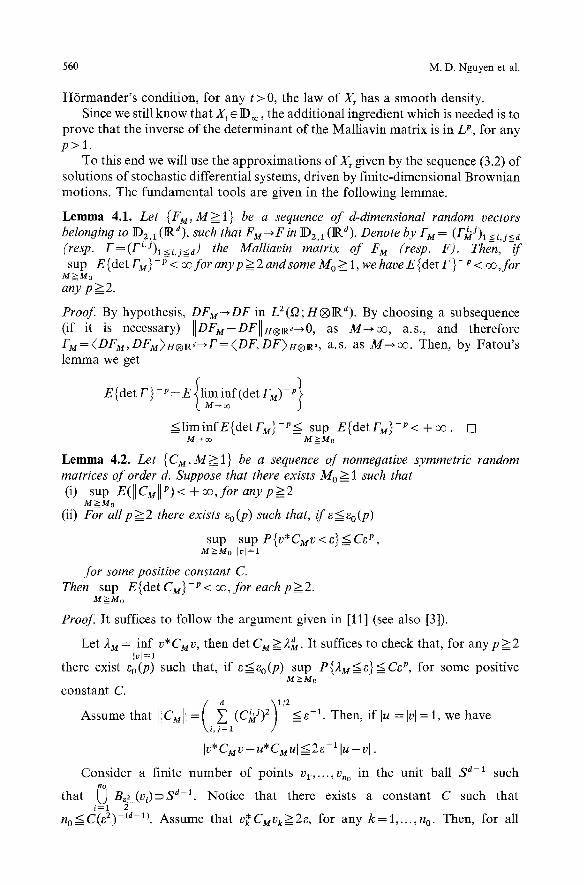
H6rmander's condition, for any t > 0, the law of Jft has a smooth density. Since we still know that X t ~ D~ , the additional ingredient which is needed is to

prove that the inverse of the determinant of the Malliavin matrix is in L p, for any p > l .

To this end we will use the approximations of X, given by the sequence (3.2) of solutions of stochastic differential systems, driven by finite-dimensional Brownian motions. The fundamental tools are given in the following lemmae.

Lemma 4.1. Let { F u , M > I } be a sequence of d-dimensional random vectors belonging to ID2,1 (IRd), such that FM~F in ID2,1 (IRd). Denote by F M = (F~J)I <=i,j<=d (resp. F=(Fi'J)l<=i,j<=d ) the Malliavin matrix of F M (resp. F). Then, if sup E { det Fu}-v < oe for any p > Zandsome Mo> 1, wehave E { det F }-P < o% for

M > M o

any p >2.

Proof. By hypothesis, DFM~DF in Lz(f2;H@IRd). By choosing a subsequence (if it is necessary) [[DF~t-DFI[~I| as M ~ o e , a.s., and therefore FM=(DFu,DFM)H| DF)I4| a.s. as M ~ o o . Then, by Fatou's lemma we get

E { det F }- V = E { lim inf ( det FM) - p}

<=liminfE{detFM}-P<= sup E{detFM}-P<+oe. [] M~oo M > M o

Lemma 4.2. Let {CM,M>I} be a sequence of nonnegative symmetric random matrices of order d. Suppose that there exists M o > 1 such that (i) sup E(IlcMIIP)< +oe,for anyp>2

M>-Mo

(ii) For all p >2 there exists eo(p) such that, if e<eo(p)

sup sup P{v*C~tv<e}<=Ce p, M > M o I v l = l

for some positive constant C. Then sup E{det CM}-P < oe, for each p > 2.

M>=Mo

Proof. It suffices to follow the argument given in [11] (see also [3]).

Let 2 u = inf V'Cur, then det CM=>2}. It suffices to check that, for a n y p > 2 Ivl =1

there exist COCO) such that, if e<eo@) sup P{2~<e}<=Ce p, for some positive M>=Mo

constant C. / / d x~l/2

Assume tha Z T en, tul=H=' , we ave i,

Iv*CMV--U*CMul<2~ llu--vl.

Consider a finite number of points v~ ..... v,o in the unit ball S ~-1 such no

that ~J B~ (v~)~S d-1. Notice that there exists a constant C such that i = 1 2

no<=C(e2) -~d-1). Assume that v~C~tvk>--_2e, for any k = l ..... n o. Then, for all


82 y e s a-1 with 7v-v~l<-f it holds that

v*CMv >=v* CMV~--IV*CMV --V* C~vkl >= e.

Consequently

P { 2 M < e } = P ~ inf v*CMv<e} {Ivl=l

=<P ~ inf v*CMv<e, IIcMll =< -l +p{iicMil > ~-1)

Uvl =1 3

n0 < Y, P{v*CMv~<2e}+e'E(llC~l[~),

k=l

and the result follows. []

In the sequel we denote by F o the vector field Fo - �89 f FVFk �9 Notice that due

f k=l to condition (B) the series F~Fk(X ) is absolutely convergent.

k=l We introduce H6rmander 's condition as follows

(H): The vector space spanned by the vector fields

F k , k > l ; [Fk,,Fk2l, kx,k2>O .... ; [...[Fk,_,,fk, l . . .],k 1 ..... k~>O ....

evaluated at x o has dimension d. We can now state the main result.

Theorem 4.3. Assume that the coefficients of the stochastic differential system satisfy hypotheses (B) and (H). Then, for any t > O, the taw of the d-dimensional random vector X t possess a (goo density with respect to the Lebesgue measure on IR d.

Before giving the proof of this theorem we will establish a modification of the crucial result of Norris (see Lemma 4.1 [7]).

Lemma 4.4. Let ~, y ~ IR. Let fl(t), 7(t) = (71 (t) . . . . . yd(t)), andu(t) = (u 1 (t) ..... ud(t)) be predictable processes. Let

t t

a(t)=~+~/~(s)ds+~ 7~(s)dB~, 0 0

and t t

r,=y+~ a(~)ds+~ ~(s)dB~s. 0 0

Assume that there exist t o ~ T and p > 2 such that

c=E{o<t<t==oSUp (lfl(t)l+[y(t)l+[a(t)l+lu(t)l)p}< + oo. (4.1)


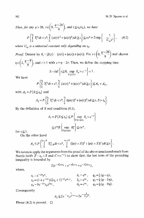
Then, for any q> 26, v6(O, @ ) , and e<%(to), we have

P{ i yt2dt<eq'! ('a(t)'2+'u(t)'2)dt~e}<=cgP+2exp{-+} ' (4.2)

where Cto is a universal constant only dependin 9 on t o.

Proof. Denote by Ot=,fi(t)l+lT(t)l+la(t)l+[u(t),. Fix r e ( 0 , q-~926-) and choose \ /

q e ( 2 , ~ ) , and r > l with v = t / - 2 r . Then, we define the stopping time

We have

P{t i yt2dt<eq,! (,a(t),2+[u(t),2)dt>@<Aa+A2,

with A l =P{S<= to} and

A2=P yt2dt<e q, ~ ([a(t)[2 +lu(t)12)dt>e,S>to . 0

By the definition of S and condition (4.1),

A~=P{S<to}<P ~ sup 0~>e-~t _ _ to__<s__<t ~ )

<erpE{o<-_~<-_toSUp OPt<ceP,) for 5<1.

On the other hand

(toAS tOAS t A2<PI ! YtZsdt<eq' 0 ~ (Ic~(tAg)12+[u(tAS)lN)dt>e "

We can now apply the arguments from the proof of the above mentioned result from Norris (with T = t o/x S and C = e -r) to show that, the last term of the preceding inequality is bounded by

2 (e - 021/2 e t ~_ e - a~/2 ~2 + e- al/2 ~3),

where,

e 1 =e--2req, 51 =eql, ql = � 8 9 e2=( l +e-2r)(2to+l)~/z~ql/2, 62=e q2, qz=~(q - -5 t l ) ,

e3 =9e-Zrto ezqz , 63----eq3 , q3 =~ (q--9t/).

Consequently 1 1

A2<2e c,S-2r=2e c,S.

Hence (4.2) is proved. []


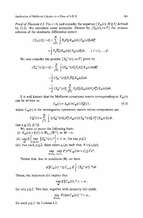
Proof of Theorem 4.3. Fix t > 0, and consider the sequence {XM(t), M> 1} defined by (3.2). We introduce some notations. Denote by {YM(t),tsT} the process solution of the stochastic differential system

M

(YM(t))~=6~ + ~ i VhF~(XM(S))(YM(S)) hdBk k = l 0

t

+I VhPiO(XM(S))(YM(s))~ ds, i, E= 1 ..... d. 0

We also consider the process { y~l ( t ) , t e T} given by

M t

(r~ 1 (t))~ = 6~- Z ~ (r~ 1 (s))} VeF~(XM(s))dB ~ k = l 0

t

-S l(s))} V Pg(XM(s))ds 0

t M

+S Z 0 k = l

It is well known that the Malliavin covariance matrix corresponding to XM(t ) can be written as

rM(t) = YM(t)CM(t) Y*(t), (4.3)

where CM(t ) is the nonnegative, symmetric matrix whose components are

M

C~t(t) = ~, i {(YM~(r))~Fk(XM(r))(YM~(r))tk'Fk'(XM(r))} dr" j = l 0

(see e.g.[3], [11]). We want to prove the following facts:

(i) XM(t)~X(t) in ID2,1(IRd), as M ~ o o . c

(ii) supE~ sup IIYMI(t)]IP~< +o0, for any p__>2. M ( 0 - < t - < l )

(iii) For each p >__ 2, there exists eo (P) such that, if e =< ~o (P),

sup sup P{v*CM(t)v<e} <=Ce p. M>-ko ] v [ = l

Notice that, due to condition (B), we have

EllcM(t)II <=C ,,,,E i llY~X(r)ll2~dr. 0

Hence, the statement (ii) implies that

sup EIIcM(t)II" < + oo, M

for any p > 2. This fact, together with property (iii) yields

sup E{det CM(t)}-P < co, M>ko

for each p > 2 , by Lemma 4.2.


Therefore, using again condition (ii) and the identity (4.3), we obtain

sup E{det Fu(t)}-P < oo, M > _ k o

for every p__> 2. Consequently, by Lemma 4.1 and property (i) we conclude that E{det F(t)} -P < 0% for anyp __> 2, where F(t) is the Malliavin matrix of the random vector X,.

Since it has been proved in Theorem 3.2 that XtelDoo(iRe), this is enough to ensure the conclusion of the Theorem.

Proof of (i). In the proof of Theorem 3.2 we have established that XM(t)-~X t in LP((2; IRa), as M--+ oo, and Xe Doo (L 2 (T; IRa)). Furthermore, for each fixed M_>_ 1

M t

D~X~(t)=F/(XM(r))+ Z ~ J ' < k VcF~(XM(s))DrX~t(s)dBs k = l r

t

+ I V<~o(XM(~))D~X~(~)ds, r

if t>=r, i=1 .. . . . M,j=I .... ,d, and D~XJM(t)=O if either r>t or i>M. On the other hand, by Proposition 2.2 we have

D~xJ(t)=FZ(X(r))+ ~ i V<F~(X(s))D~X<(s)dB~ k = l r

t

+ ~ V<P~o(X(s))D~X<(s)ds. r

We next prove that

lira ]IDXM(t)--DX(t)HL2(O;H| (4.4)

where H=LE(T• Z+ ; IR). Indeed,

where 1

A~t=E ~ 0

A~,=E} 0

A~t=E } 0

A~=E} 0

A~t=E } 0

E~ ~, [D~X~(t)--D~,XJ(t)lEdr~ C Z A~t, 0 i = l j = l a = l

M d

Z Z i = 1 j = l

i = 1 j = l

i = l j = l

i=1 j=t

i = 1 j = l

IFi(X~(r))- Fi(X(~))I ~ dr,

j i ~ j i ~ k (V<F/~(XM(s))D,X~t(s) - V<F/,(X(s))DrX (s))dB s dr, / = 1 r

} VeF~(X(s))D~Xr k = M + l r

~' } (v<Pg(x.( '~x~( v<Pg( '~ 2 ~, s))O s)- X(s))D Xe(s))ds dr, k = l r

k = M + l r

A p p l i c a t i o n o f M a l l i a v i n C a l c u l u s to a C l a s s o f S. D . E . 565

and

1 d

A 6 = E ~ ~ 2 IF/(X(r))I zdr. 0 I = M + I j = l

Condition (L) implies that

1

A~t < KE ~ IXg(r) -X(r)lZ dr 0

_<KE~ sup [XM(r)--X(r)[ 2} - - {O_<r_< 1

and this last expression tends to zero as M ~ o% as has been established in the proof of Theorem 3.2.

2 < 1 2 For A~ we have AM= C{BM+BM}, with

1 ~ ~ [ M i VeF~(X(s)))DiX~(s)dB 2dr B~t =E ! 2 (VeF/(XM(S))- i = 1 j = l k = l r

and

B2=E ~ j i ~ i e k I

0 i = 1 j = l k = l r

Burkholder's inequality yields

0 i = 1 j = l k = l r

On the other hand, using condition (B), the second term of this inequality can be bounded by

1 t d

CK, E I I IXM(S)--X(s)I z ~ Z [D~Xfu(s)[ 2dsdr, 0 r i = 1 d = l

and by Schwarz inequality this is less or equal than

sup sup sup sup f f \ (O--<s--<l M r [.r<s<-_l i = 1 d = l

The second factor of this expression is bounded [see (3.6)]. Consequently lim B~=0.

M ~ o o

Wenow take care of B~. By Burkholder's inequality and condition (B) we obtain

<=CK, E i e -D~Xe(s)lZdr ds 0 i=1 t = l

t

= c~, I IIDXM(~) -- DX(~)[I~(~;, , | 0


Using the same arguments we get

A~<=CE ~ 2 IVeF;k(X(s))l 2 ID~X~(s)12ds dr 0 i = 1 j = l k = M + l

<sup sup ~ IWeF~(x)12supE sup IDjX*(s)l 2 (4.5) x l < d < d j = l k = M + l r ~r<s<l i = 1 d = l

The second factor of (4.5) is bounded because of (3.6), while the first one tends to zero as M ~ ~ , due to condition (B).

For A~ (resp. A~), we have analogous results than for A~ (resp. A~). Finally, it is clear that condition (B) ensures lim A 6 = 0.

M--* oo

Therefore, we have proved that

<= C~, {C~,+ i llDXM(s)-DX(s)ll%2(~;~om,~ds } with lim CM = 0, and consequently, using Gronwall's lemma we obtain (4.4). This

M--* a|

finishes the proof of statement (i).

Proof of (ii). Burkholder and H61der's inequalities, together with condition (B) imply

{ ( 1 "~p/2 i , d = l k = l 0 j = l j = l

\p/2 i,t=l j=l ~=1 [VtFd(XM(s))12ds/ !

+ Z E [(YM~(S))~] 2 Z 2 [VhF~(XM(s))[ 2 i,d=l j=l j,h=l k=l

�9 ~, IV~Fg(XM(S))I2ds ~p/2) h = l k = l

=<Cp,,, K, 1 + ! E sup IIr~;~(~)ll d s . I O_<s-<l

Thus (ii) follows easily from Gronwall's 1emma.

Proof of (iii). Let us introduce the sets

Z;={Fk, k>=l},

12;= {[F,, V],k>O, Ve12,_1}, for n____l,

I 2 ' = 0 1 2 ' /1' n = 0


By H6rmander ' s condi t ion (H), the linear span of 2;' at the point x o is B~ d. Consider now a new family of vector fields, as follows,

Define

Then

Zo = 1;g

2; ={[Fk, V],k>=I, Ve2;,_~;[Fo, V]+�89 ~ [Fj,[Fj, V]],Ve1;._I}, n>l j = l

2 ; = 0 2;,. n=0

Notice that, using condi t ion (B), it can be checked recursively that the vector fields

~, [Fj, [Fj, V]] are well-defined. j = l

We want to show that the linear span of 2; at point x o is N d. To this end we will check that i fv e IR e is or thogonal to any vector in 1; (xo) , then v is also or thogonal to I;'(Xo), and hence v = 0.

Let V62;[,, V=[Fk.,[Fk.-1,...,[Fk2,Fkl]...]], with k a > l and k 2 . . . . . k , > 0 . Assume that the indices k jl . . . . . k jr are zero (r < n). For the sake of simplicity we will only consider the case r = 2. Then

V=[Fk.,[...[Fo,[FG-I,[ .... [F0, H2I...], ] ] . . . l ]

with Hz= [FG_I, [ .... [Fk2,F,,]...]] El;. We write V= Vt - V2, where

V~ = [Fk,, [... [F o, [Fk, l - 1, [ .... [Fo, H 2 ] + �89 ~ [Fj, [ r j , / /21 ]-.-1, ] 1... ] ] j = l

V2 = [Fk, , [... [ro, [FG_I , [ .... �89 ~ [r j , [Fj, H2]]...]. j= l

H I = [ F G _ I , [ .... [Fo,Hz]+�89 [Fj,[Fj, Ha]]...]]. Notice that H l e Z . j=l

v~ = [rk., [ . . . [ r 0 , H d + k ~ [Fh, [ G , H d ] . . . ] ] h = l

- [rk., [ .... } ~ [G, [G, HI]]...]]. h : l

On the other hand, by putt ing

we have

~;=[F~,_,,[ .... } Z [Fj,[rj,/-6]]...]], j = l

V:=[F~,,[...[Fo, Hfl+k ~ [F~,[F~,H;]]...]] h= l

-[F,~,,[.:.,�89 ~ [F,,,[Fh,H~]]...]]. h = l


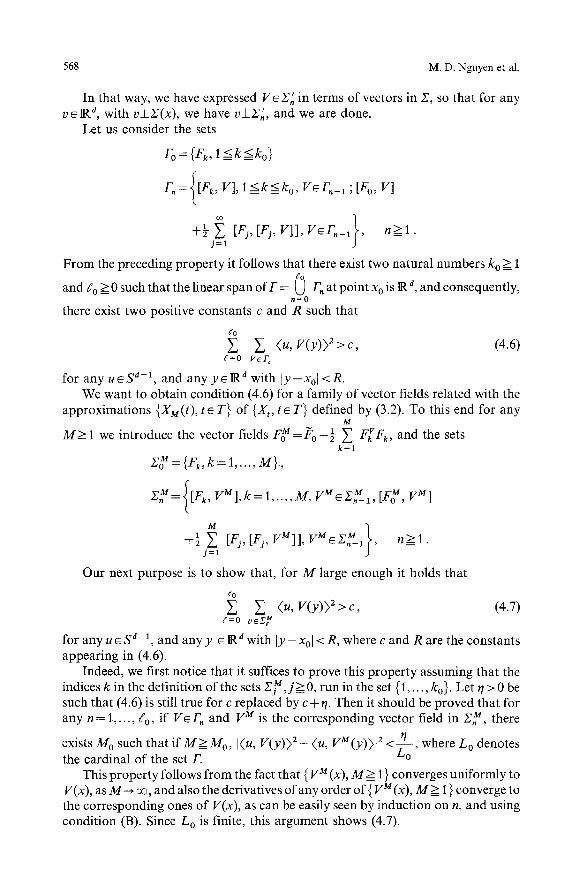
In that way, we have expressed Ve X~ in terms of vectors in Z, so that for any v~lR d, with v_LX(x), we have v_l_X[,, and we are done.

Let us consider the sets

ro= {rk, l <__k <=ko}

F n={[F k, V], 1 <=k<k o, V~Fn_ 1 ; [F o, V]

+2 t- ~ [Fj, [Fj, V]], V~F~_I}, n>=l. j = l

From the preceding property it follows that there exist two natural numbers k o > 1 go

and fo => 0 such that the linear span of F = U Fn at point x o is IRa, and consequently, n=0

there exist two positive constants c and R such that

r ~ (u, V(y)) 2 > c , (4.6)

d=o VEG

for any u~S a-l, and any yEIR d with ]y-xol <R. We want to obtain condition (4.6) for a family of vector fields related with the

approximations {XM(t), t~ T} of {Xt, t~T} defined by (3.2). To this end for any M

M_->I we introduce the vector fields F ~ - - P 0 - � 8 9 ~, F~Fk, and the sets k=l

X ~ = {F k, k = 1 . . . . . M } ,

Xy={[F k, V~t], k = 1 ..... M, vME~-,nM_I, [Fg, V M ]

+21 .#=1 ~ [Fj'[Fj'VM]]'VM~X~-'} ' n>=l.

Our next purpose is to show that, for M large enough it holds that

~'o 2 2 (U, V(y ) ) 2 > c , (4.7)

t=0 v~2;e ~

for any u ~ S d-l , and any y ~ IR d with [y -Xo[ < R, where c and R are the constants appearing in (4.6).

Indeed, we first notice that it suffices to prove this property assuming that the indices k in the definition of the sets Zfft,j>O, run in the set {1 ... . . ko}. Let r/> 0 be such that (4.6) is still true for c replaced by c + t/. Then it should be proved that for any n = l .... , Eo, if V~F, and V u is the corresponding vector field in Z y , there

exists M o such that if M > M o , [(u, V(y)) 2 - (u, VM(y))[ 2 <q----, where L o denotes the cardinal of the set F. ~ o

This property follows f rom the fact that { VM(x), M > 1 } converges uniformly to V(x), as M ~ 0% and also the derivatives of any order of { V M (x), M > 1 } converge to the corresponding ones of V(x), as can be easily seen by induction on n, and using condition (B). Since L o is finite, this argument shows (4.7).


From (4.7) it follows that there exists a vector field Vjo s sjMo, withjo < fo such that

(v* Vjo (y)) 2 =>~o = c ' , (4.8)

for any yeS d-l, and every y e l R d, with ]y-Xo]<=R. Consider the decreasing sequence of real numbers defined by ~ (j) = 2-5 j. First

we prove that, for any p >_ 2, there exists e o (p) such that, if e =< e o (p),

P{i (v*YTtl(s)Vj~176 <=Cpep' (4.9)

for any yeS d-a, where Cp do not depend on M. Indeed, let us introduce the stopping time given by

SM=inf { a>O' o~=s~=~sup [XM(s)-xol> R, or o~s_~sup l]Y~l(s)-l][>�89

Fix Be(0, ~(eo)), and write Gjo= (v*Y~l(s)Vjo(XM(S)))2ds<e "~(i~ . Then

P(G2o) <-_P(GjoC~{SM >= eP}) + P {SM < er For e small enough, the set GjoC~{SM>e p} is empty. In fact, on Fjo we have

i (v* Y~ 1 (s) Vjo (X M (s))) 2 ds < e ~ (Jo) __< e'*(e~ (4.10) 0

On the other hand, on {SM>__e~},

SM

i (v, 0 0

C'~/~ - - - - - (4.11) - - 4 '

due to condit ion (4.8) and the definition of S M. Choosing ~ and fl in an appropriate way, we see that (4.10) and (4.11) are

contradictory. M o r e o v e r ,

P{SM<e~} <P(( ~ [X~(s)--Xo[>R, or o_<~_<~.sup IIYffl(s)-I[[>�89

=~<1 E~(o_<~sup IXM(s)--Xo[P~+2PEt) (0-<~-<~sup I[Y~a(s)--I]I v}

<- C v e p~/2. This last estimation is obtained by standard arguments. We notice that, due to condit ion (B) the constant Cv does not depend on M. Consequently (4.9) is proved.

The vector field Vjo M" 2:jo IS either of the form [Fk, Vjo_ a ], for some k -- 1 . . . . . M o r M

[Fo M, Vfo_~]-t- �89 ~ [Fj, [Fj, Vj'o_l]], with Vjo_ ] . . . . M , Vjo_ ~ e Z, jo_ 1, and so on. j = l

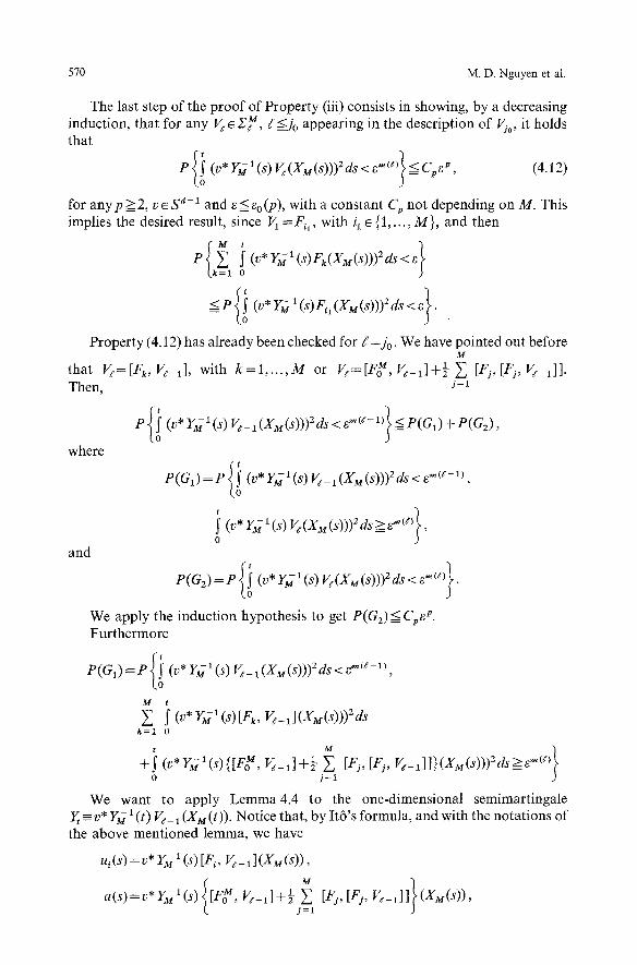
570 M . D . N g u y e n et al.

The last step of the proof of Property (iii) consists in showing, by a decreasing induction, that for any V t e 2;~, #<Jo appearing in the description of V~o, it holds that

P { i (v* YFt~(s) V~(XM(s)))2 ds < e~t)} <=Cp~p' (4.12)

for any p > 2, v e S d- ~ and e < ~0 (P), with a constant C v not depending on M. This implies the desired result, since V 1 =F~, with i~ E {1 ..... M}, and then

P (v*Y~l(s)fk(XM(s)))2ds<e k 0

<P{i (v*yffl(s)Fil(Xm(S)))2ds<~}" ,

Property (4.12) has already been checked for ~ =Jo. We have pointed out before M

that V~=[Fg, Ve_~], with k = l ..... M or V~=[F~, Ve_~]+ ~ ~ [Fj, [Fj, Ve_l]]. Then, j = 1

P{i (V*YM~(S)V~-~(XM(s)))2ds<e'~(~-~)} <=P(G1)+P(G2)' where

and

P(G~)=P{i (T)*yMI(s)Vd-I(XM(S))) 2dS'~e~(~-l) ,

i (v* Y~ ~ (s) Vt(XM(s)))2 ds > e~(t)} ,

P(G2)=P{i (v*YMI(s) V~(XM(S)))2ds<e'~(e)} �9

We apply the induction hypothesis to get P(G2)_< Cpe p. Furthermore

M

Y, i (v* ry,'(s)[f~, V~_l](X~(s)))2ds k = l 0

} +~ (v*Y~(s){[FY, b-~]+~ ~ [Fj, [F~, ~_~]]}(XM(s)))2ds_-->~ ~'~ 0 j = l

We want to apply Lemma4.4 to the one-dimensional semimartingale -v* Y~2 ~ (t) V t_ ~ (XM(t)). Notice that, by It6's formula, and with the notations of

the above mentioned lemma, we have

u i (s) = v* YM 1 (S) [Fi, V t_ t ] (XM (S)),

a(s)=v* yMI(s){ [F~ V~-a]+�89 ~j=l [Fj'[Fj' V~-a]]} (Xg(s))'


and

7i(s)=v* y~tl(s){ [Fi' [Fg' Ve-1]]-}-�89 ~j=l [Fi' [Fj' [Fj' Ve-1]]]} (XM(S))'

f M [Fg, [Fg, V _d]+�89 Z [Fj, [Fj, j = l

h = l j = l

Straightforward computations show that the inequality (4.1) is satisfied for any p > 2 and t o e T. Moreover, due to condition (B) the constant c of (4.1) does not depend on M. Therefore, using (4.2), we obtain that, for anyp >2 there exists co(p) such that, for any ~ < co(p), P(G1)< Cpe p. This finishes the proof of the inductive step and of the theorem. []

References

1. Bouleau, N., Hirsch, F. : Propri6t6s d'absolue continuit6 dans les espaces de Dirichlet et application aux 6quations diff~rentielles stochastiques. S~minaire de Probabilit~s XX. (Lect. Notes Math., vol. 1204, pp. 131-161) Berlin Heidelberg New York: Springer 1980

2. Carmona, R., Nualart, D. : Nonlinear stochastic integrators, equations and flows. Stochastics monographs. London New York: Gordon and Breach (to appear)

3. Ikeda, N., Watanabe, S. : Stochastic differential equations and diffusion processes. Amsterdam Oxford New York: North Holland/Kodansha 1981

4. Kunita, H. : Lectures on Stochastic flows and applications. Lect. Math. Phys., Math., Tata Inst. Fundam. Res. Berlin Heidelberg New York: Springer 1983

5. Le Jan, Y., Watanabe, S. : Stochastic flows of diffeomorphisms. Stochastic Analysis. Proceedings of the Taniguchi Conference, Kyoto 1982. Amsterdam New York Oxford: North Holland 1984

6. Millet, A., Nualart, D , Sanz, M. : Time reversal for infinite-dimensional diffusions. Probab. Th. Rel. Fields 82, 315-347 (1989)

7. Norris, J. : Simplified Malliavin calculus. S~minaire de Probahilit6s XX. (Lect. Notes Math., vol. 1204, pp. 101-130) Berlin Heidelberg New York: Springer 1986

8. Nualart, D., Zakai, M. : Generalized stochastic integrals and the Malliavin calculus. Probab. Th. Rel. Fields 73, 255-280 (1986)

9. Nualart, D., Zakai, M. : Generalized multiple stochastic integrals and the representation of Wiener functionals. Stochastics 23, 311-330 (1988)

10. Nualart, D., Pardoux, E. : Stochastic calculus with anticipating integrands. Probab. Th. Rel. Fields 78, 535-581 (1988)

11. Stroock, D.W. : Some applications of stochastic calculus to partial differential equations. Ecole d'6t~ de Probabilit~s de Saint-Flour XI, 1981. (Lect. Notes Math., vol. 976, pp. 268-382) Berlin Heidelberg New York: Springer 1983

12. Sznitman, A.S. : Martingales d~pendant d'un param6tre: une formule d'It6. Z. Wahrscheinlich- keitstheor. Verw. Geb. 68, 41-70 (1982)

Received March 21, 1989; in revised form September 19, 1989

Application of Malliavin calculus to a class of stochastic differential equations

Documents

Transcript of Application of Malliavin calculus to a class of stochastic differential equations