Application of Machine Learning Techniques for Heart...
7
Abstract—Ultrasound and electrocardiogram (ECG) are standard, reputable methods for heart disease diagnosis, but due to expensive and limited accessibility, typical preliminary diagnosis are performed by highly trained physicians with stethoscope hearings. Due to global shortage of healthcare providers, there is growing interest for a cheaper, more ubiquitous alternative. The envisioned goal is to determine, from a single short 5 - 120 sec precordial heart sound recording, whether the patient should be referred to expert diagnosis. Such heart sound recordings can come from various clinical or nonclinical environments, including at-home recordings with a smartphone to in-hospital recordings by a nurse. For diagnosis to be successfully automated, heart sound waveforms must be segmented into appropriate S1, systole, S2, and diastole phases of the heart cycle. In this paper, logistic regression hidden semi-Markov model is used for waveform segmentation. Features are then extracted from the segmented waveforms and used in conjunction with physician-provided classification labels, to train supervised machine learning models to identify heart abnormality in patient test data. Various supervised machine learning models are explored, implemented, and compared for performance. Index Terms—Heart sound segmentation, hidden Markov models, (HMMs), logistic regression (LR), phonocardiography (PCG), feature extraction, heartbeat time series, heart rate variability (HRV), support vector machine (SVM). I. INTRODUCTION HEART sound recording can be an inexpensive way to acquire patients' heart rate variability (HRV) information, compared with more involved techniques such as electrocardiogram (ECG) at the hospital. Audio recording with a smartphone or a voice recorder can readily be achieved at home, providing an affordable way to collect valuable patient information. Prior research has shown HRV can be used to classify patients’ physiological condition, age, autonomic nervous balance, level of stress and activity [1]. We used publicly available heart sound recordings [2, 3] to classify whether a patient has normal or abnormal heart condition, e.g. heart murmur or extrasystole heartbeat. Our approach applies techniques discussed in [1] to phonocardiograms (PCG), instead of ECG waveforms. We will use datasets available in [2, 3] to create a model for classifying PCG into two different classes: normal or abnormal. We conducted pre-processing of audio samples into PCG features, which are then used in heart sound classification. In particular, segmentation of time series data into four distinctive phases of a heartbeat cycle, the S1 (lub) and S2 (dub) sounds and the systole and diastole periods between them, is required to extract HRV features for PCG classification. S1 and S2 respectively mark the beginning of systole and diastole phases of a heartbeat, as shown in Figure 1 below. We use logistic regression hidden semi-Markov model [4, 5] to segment heartbeat waveforms into four states, as this algorithm is currently state-of-the-art. Figure 1: Illustration of simultaneously recorded PCG and ECG waveforms with labels of S1, systole, S2, and diastole states of the heart cycle. Note the R- peak and T-wave end markers in ECG correspond to approximate S1 and S2 positions. ECG is used as the reference and considered more accurate than PCG. Figure is taken from reference [5] for illustration purposes. Once data is segmented, we extract statistical HRV features and use several supervised learning methods to classify waveforms into two classes as described above. Support vector machines (SVM) is shown as a robust and efficient technique for classifying ECG signals based on HRV analysis [1]. Moreover, SVMs remained robust even with white Gaussian noise added to the waveforms. Other classifiers considered are logistic regression, neural network, and K-means clustering. The flowcharts in Figure 2 and Figure 3 respectively illustrate the steps for LR-HSMM creation and its application in the overall classification scheme. This paper is organized as follows: Section II describes dataset preparation and preprocessing necessary for correct waveform segmentation. Section III describes HRV features extraction for classification. Section IV presents classification algorithms. Section V discusses classification model performance and error analysis. Section VI concludes the paper. II. DATASET PREPARATION AND PREPROCESSING Our heart sound dataset consists of five databases labeled A through E, containing a total of 3,541 heart sound recordings in .wav format, each lasting between 5 to over 120 seconds. Sound recordings are provided by Physionet [3], come from a variety of environments and patients, and are recorded from various locations on the body. The recordings are labeled as either Anatoly Yakovlev, SUNet ID: yakovlev, Student ID: 05536959 Vincent Lee, SUNet ID: vclee, Student ID: 05372645 Application of Machine Learning Techniques for Heart Sound Recording Classification
Transcript of Application of Machine Learning Techniques for Heart...

Abstract—Ultrasound and electrocardiogram (ECG) are
standard, reputable methods for heart disease diagnosis, but due
to expensive and limited accessibility, typical preliminary
diagnosis are performed by highly trained physicians with
stethoscope hearings. Due to global shortage of healthcare
providers, there is growing interest for a cheaper, more ubiquitous
alternative. The envisioned goal is to determine, from a single
short 5 - 120 sec precordial heart sound recording, whether the
patient should be referred to expert diagnosis. Such heart sound
recordings can come from various clinical or nonclinical
environments, including at-home recordings with a smartphone to
in-hospital recordings by a nurse. For diagnosis to be successfully
automated, heart sound waveforms must be segmented into
appropriate S1, systole, S2, and diastole phases of the heart cycle.
In this paper, logistic regression hidden semi-Markov model is
used for waveform segmentation. Features are then extracted
from the segmented waveforms and used in conjunction with
physician-provided classification labels, to train supervised
machine learning models to identify heart abnormality in patient
test data. Various supervised machine learning models are
explored, implemented, and compared for performance.
Index Terms—Heart sound segmentation, hidden Markov models,
(HMMs), logistic regression (LR), phonocardiography (PCG),
feature extraction, heartbeat time series, heart rate variability
(HRV), support vector machine (SVM).
I. INTRODUCTION
HEART sound recording can be an inexpensive way to
acquire patients' heart rate variability (HRV) information,
compared with more involved techniques such as
electrocardiogram (ECG) at the hospital. Audio recording with
a smartphone or a voice recorder can readily be achieved at
home, providing an affordable way to collect valuable patient
information. Prior research has shown HRV can be used to
classify patients’ physiological condition, age, autonomic
nervous balance, level of stress and activity [1]. We used
publicly available heart sound recordings [2, 3] to classify
whether a patient has normal or abnormal heart condition, e.g.
heart murmur or extrasystole heartbeat.
Our approach applies techniques discussed in [1] to
phonocardiograms (PCG), instead of ECG waveforms. We will
use datasets available in [2, 3] to create a model for classifying
PCG into two different classes: normal or abnormal. We
conducted pre-processing of audio samples into PCG features,
which are then used in heart sound classification. In particular,
segmentation of time series data into four distinctive phases of
a heartbeat cycle, the S1 (lub) and S2 (dub) sounds and the
systole and diastole periods between them, is required to extract
HRV features for PCG classification. S1 and S2 respectively
mark the beginning of systole and diastole phases of a heartbeat,
as shown in Figure 1 below. We use logistic regression hidden
semi-Markov model [4, 5] to segment heartbeat waveforms into
four states, as this algorithm is currently state-of-the-art.
Figure 1: Illustration of simultaneously recorded PCG and ECG waveforms
with labels of S1, systole, S2, and diastole states of the heart cycle. Note the R-
peak and T-wave end markers in ECG correspond to approximate S1 and S2 positions. ECG is used as the reference and considered more accurate than
PCG. Figure is taken from reference [5] for illustration purposes.
Once data is segmented, we extract statistical HRV features
and use several supervised learning methods to classify
waveforms into two classes as described above. Support vector
machines (SVM) is shown as a robust and efficient technique
for classifying ECG signals based on HRV analysis [1].
Moreover, SVMs remained robust even with white Gaussian
noise added to the waveforms. Other classifiers considered are
logistic regression, neural network, and K-means clustering.
The flowcharts in Figure 2 and Figure 3 respectively illustrate
the steps for LR-HSMM creation and its application in the
overall classification scheme.
This paper is organized as follows: Section II describes
dataset preparation and preprocessing necessary for correct
waveform segmentation. Section III describes HRV features
extraction for classification. Section IV presents classification
algorithms. Section V discusses classification model
performance and error analysis. Section VI concludes the paper.
II. DATASET PREPARATION AND PREPROCESSING
Our heart sound dataset consists of five databases labeled A
through E, containing a total of 3,541 heart sound recordings in
.wav format, each lasting between 5 to over 120 seconds. Sound
recordings are provided by Physionet [3], come from a variety
of environments and patients, and are recorded from various
locations on the body. The recordings are labeled as either
Anatoly Yakovlev, SUNet ID: yakovlev, Student ID: 05536959
Vincent Lee, SUNet ID: vclee, Student ID: 05372645
Application of Machine Learning Techniques
for Heart Sound Recording Classification
normal or abnormal, with no distinction among the various
heart diseases. There are 2,725 normal and 816 abnormal
recordings which are shuffled into training and test datasets.
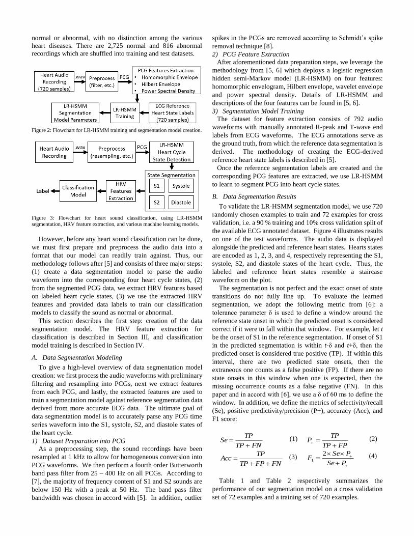
Figure 2: Flowchart for LR-HSMM training and segmentation model creation.
Figure 3: Flowchart for heart sound classification, using LR-HSMM segmentation, HRV feature extraction, and various machine learning models.
However, before any heart sound classification can be done,
we must first prepare and preprocess the audio data into a
format that our model can readily train against. Thus, our
methodology follows after [5] and consists of three major steps:
(1) create a data segmentation model to parse the audio
waveform into the corresponding four heart cycle states, (2)
from the segmented PCG data, we extract HRV features based
on labeled heart cycle states, (3) we use the extracted HRV
features and provided data labels to train our classification
models to classify the sound as normal or abnormal.
This section describes the first step: creation of the data
segmentation model. The HRV feature extraction for
classification is described in Section III, and classification
model training is described in Section IV.
A. Data Segmentation Modeling
To give a high-level overview of data segmentation model
creation: we first process the audio waveforms with preliminary
filtering and resampling into PCGs, next we extract features
from each PCG, and lastly, the extracted features are used to
train a segmentation model against reference segmentation data
derived from more accurate ECG data. The ultimate goal of
data segmentation model is to accurately parse any PCG time
series waveform into the S1, systole, S2, and diastole states of
the heart cycle.
1) Dataset Preparation into PCG
As a preprocessing step, the sound recordings have been
resampled at 1 kHz to allow for homogeneous conversion into
PCG waveforms. We then perform a fourth order Butterworth
band pass filter from 25 – 400 Hz on all PCGs. According to
[7], the majority of frequency content of S1 and S2 sounds are
below 150 Hz with a peak at 50 Hz. The band pass filter
bandwidth was chosen in accord with [5]. In addition, outlier
spikes in the PCGs are removed according to Schmidt’s spike
removal technique [8].
2) PCG Feature Extraction
After aforementioned data preparation steps, we leverage the
methodology from [5, 6] which deploys a logistic regression
hidden semi-Markov model (LR-HSMM) on four features:
homomorphic envelogram, Hilbert envelope, wavelet envelope
and power spectral density. Details of LR-HSMM and
descriptions of the four features can be found in [5, 6].
3) Segmentation Model Training
The dataset for feature extraction consists of 792 audio
waveforms with manually annotated R-peak and T-wave end
labels from ECG waveforms. The ECG annotations serve as
the ground truth, from which the reference data segmentation is
derived. The methodology of creating the ECG-derived
reference heart state labels is described in [5].
Once the reference segmentation labels are created and the
corresponding PCG features are extracted, we use LR-HSMM
to learn to segment PCG into heart cycle states.
B. Data Segmentation Results
To validate the LR-HSMM segmentation model, we use 720
randomly chosen examples to train and 72 examples for cross
validation, i.e. a 90 % training and 10% cross validation split of
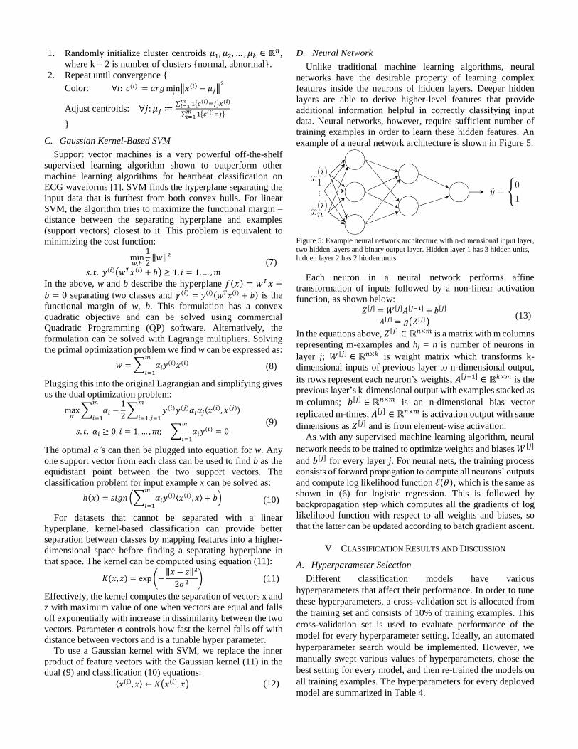
the available ECG annotated dataset. Figure 4 illustrates results
on one of the test waveforms. The audio data is displayed
alongside the predicted and reference heart states. Hearts states
are encoded as 1, 2, 3, and 4, respectively representing the S1,
systole, S2, and diastole states of the heart cycle. Thus, the
labeled and reference heart states resemble a staircase
waveform on the plot.
The segmentation is not perfect and the exact onset of state
transitions do not fully line up. To evaluate the learned
segmentation, we adopt the following metric from [6]: a
tolerance parameter δ is used to define a window around the
reference state onset in which the predicted onset is considered
correct if it were to fall within that window. For example, let t
be the onset of S1 in the reference segmentation. If onset of S1
in the predicted segmentation is within t-δ and t+δ, then the
predicted onset is considered true positive (TP). If within this
interval, there are two predicted state onsets, then the
extraneous one counts as a false positive (FP). If there are no
state onsets in this window when one is expected, then the
missing occurrence counts as a false negative (FN). In this
paper and in accord with [6], we use a δ of 60 ms to define the
window. In addition, we define the metrics of selectivity/recall
(Se), positive predictivity/precision (P+), accuracy (Acc), and
F1 score:
FNTP
TPSe
(1)
FPTP
TPP
(2)
FNFPTP
TPAcc
(3)
PSe
PSeF
21
(4)
Table 1 and Table 2 respectively summarizes the
performance of our segmentation model on a cross validation
set of 72 examples and a training set of 720 examples.
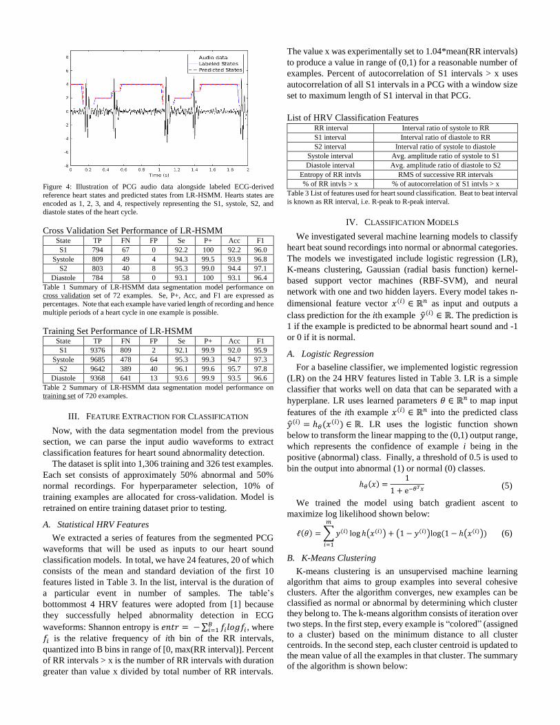
Figure 4: Illustration of PCG audio data alongside labeled ECG-derived
reference heart states and predicted states from LR-HSMM. Hearts states are
encoded as 1, 2, 3, and 4, respectively representing the S1, systole, S2, and diastole states of the heart cycle.
Cross Validation Set Performance of LR-HSMM
State TP FN FP Se P+ Acc F1
S1 794 67 0 92.2 100 92.2 96.0
Systole 809 49 4 94.3 99.5 93.9 96.8
S2 803 40 8 95.3 99.0 94.4 97.1
Diastole 784 58 0 93.1 100 93.1 96.4
Table 1 Summary of LR-HSMM data segmentation model performance on cross validation set of 72 examples. Se, P+, Acc, and F1 are expressed as
percentages. Note that each example have varied length of recording and hence
multiple periods of a heart cycle in one example is possible.
Training Set Performance of LR-HSMM State TP FN FP Se P+ Acc F1
S1 9376 809 2 92.1 99.9 92.0 95.9
Systole 9685 478 64 95.3 99.3 94.7 97.3
S2 9642 389 40 96.1 99.6 95.7 97.8
Diastole 9368 641 13 93.6 99.9 93.5 96.6
Table 2 Summary of LR-HSMM data segmentation model performance on
training set of 720 examples.
III. FEATURE EXTRACTION FOR CLASSIFICATION
Now, with the data segmentation model from the previous
section, we can parse the input audio waveforms to extract
classification features for heart sound abnormality detection.
The dataset is split into 1,306 training and 326 test examples.
Each set consists of approximately 50% abnormal and 50%
normal recordings. For hyperparameter selection, 10% of
training examples are allocated for cross-validation. Model is
retrained on entire training dataset prior to testing.
A. Statistical HRV Features
We extracted a series of features from the segmented PCG
waveforms that will be used as inputs to our heart sound
classification models. In total, we have 24 features, 20 of which
consists of the mean and standard deviation of the first 10
features listed in Table 3. In the list, interval is the duration of
a particular event in number of samples. The table’s
bottommost 4 HRV features were adopted from [1] because
they successfully helped abnormality detection in ECG
waveforms: Shannon entropy is 𝑒𝑛𝑡𝑟 = −∑ 𝑓𝑖𝑙𝑜𝑔𝑓𝑖𝐵𝑖=1 , where
𝑓𝑖 is the relative frequency of ith bin of the RR intervals,
quantized into B bins in range of [0, max(RR interval)]. Percent
of RR intervals > x is the number of RR intervals with duration
greater than value x divided by total number of RR intervals.
The value x was experimentally set to 1.04*mean(RR intervals)
to produce a value in range of (0,1) for a reasonable number of
examples. Percent of autocorrelation of S1 intervals > x uses
autocorrelation of all S1 intervals in a PCG with a window size
set to maximum length of S1 interval in that PCG.
List of HRV Classification Features RR interval Interval ratio of systole to RR
S1 interval Interval ratio of diastole to RR
S2 interval Interval ratio of systole to diastole
Systole interval Avg. amplitude ratio of systole to S1
Diastole interval Avg. amplitude ratio of diastole to S2
Entropy of RR intvls RMS of successive RR intervals
% of RR intvls > x % of autocorrelation of S1 intvls > x
Table 3 List of features used for heart sound classification. Beat to beat interval
is known as RR interval, i.e. R-peak to R-peak interval.
IV. CLASSIFICATION MODELS
We investigated several machine learning models to classify
heart beat sound recordings into normal or abnormal categories.
The models we investigated include logistic regression (LR),
K-means clustering, Gaussian (radial basis function) kernel-
based support vector machines (RBF-SVM), and neural
network with one and two hidden layers. Every model takes n-
dimensional feature vector 𝑥(𝑖) ∈ ℝ𝑛 as input and outputs a
class prediction for the ith example �̂�(𝑖) ∈ ℝ. The prediction is
1 if the example is predicted to be abnormal heart sound and -1
or 0 if it is normal.
A. Logistic Regression
For a baseline classifier, we implemented logistic regression
(LR) on the 24 HRV features listed in Table 3. LR is a simple
classifier that works well on data that can be separated with a
hyperplane. LR uses learned parameters 𝜃 ∈ ℝ𝑛 to map input
features of the ith example 𝑥(𝑖) ∈ ℝ𝑛 into the predicted class
�̂�(𝑖) = ℎ𝜃(𝑥(𝑖)) ∈ ℝ. LR uses the logistic function shown
below to transform the linear mapping to the (0,1) output range,
which represents the confidence of example i being in the
positive (abnormal) class. Finally, a threshold of 0.5 is used to
bin the output into abnormal (1) or normal (0) classes.
ℎ𝜃(𝑥) =1
1 + e−𝜃𝑇𝑥 (5)
We trained the model using batch gradient ascent to
maximize log likelihood shown below:
ℓ(𝜃) = ∑𝑦(𝑖) log ℎ(𝑥(𝑖)) + (1 − 𝑦(𝑖))log (1 − ℎ(𝑥(𝑖)))
𝑚
𝑖=1
(6)
B. K-Means Clustering
K-means clustering is an unsupervised machine learning
algorithm that aims to group examples into several cohesive
clusters. After the algorithm converges, new examples can be
classified as normal or abnormal by determining which cluster
they belong to. The k-means algorithm consists of iteration over
two steps. In the first step, every example is “colored” (assigned
to a cluster) based on the minimum distance to all cluster
centroids. In the second step, each cluster centroid is updated to
the mean value of all the examples in that cluster. The summary
of the algorithm is shown below:
1. Randomly initialize cluster centroids 𝜇1, 𝜇2, … , 𝜇𝑘 ∈ ℝ𝑛,
where k = 2 is number of clusters {normal, abnormal}.
2. Repeat until convergence {
Color: ∀𝑖: 𝑐(𝑖) ≔ 𝑎𝑟𝑔min𝑗
‖𝑥(𝑖) − 𝜇𝑗‖2
Adjust centroids: ∀𝑗: 𝜇𝑗 ≔∑ 1{𝑐(𝑖)=𝑗}𝑥(𝑖)𝑚
𝑖=1
∑ 1{𝑐(𝑖)=𝑗}𝑚𝑖=1
}
C. Gaussian Kernel-Based SVM
Support vector machines is a very powerful off-the-shelf
supervised learning algorithm shown to outperform other
machine learning algorithms for heartbeat classification on
ECG waveforms [1]. SVM finds the hyperplane separating the
input data that is furthest from both convex hulls. For linear
SVM, the algorithm tries to maximize the functional margin –
distance between the separating hyperplane and examples
(support vectors) closest to it. This problem is equivalent to
minimizing the cost function:
min𝑤,𝑏
1
2‖𝑤‖2
𝑠. 𝑡. 𝑦(𝑖)(𝑤𝑇𝑥(𝑖) + 𝑏) ≥ 1, 𝑖 = 1,… ,𝑚
(7)
In the above, w and b describe the hyperplane 𝑓(𝑥) = 𝑤𝑇𝑥 +𝑏 = 0 separating two classes and 𝛾(𝑖) = 𝑦(𝑖)(𝑤𝑇𝑥(𝑖) + 𝑏) is the
functional margin of w, b. This formulation has a convex
quadratic objective and can be solved using commercial
Quadratic Programming (QP) software. Alternatively, the
formulation can be solved with Lagrange multipliers. Solving
the primal optimization problem we find w can be expressed as:
𝑤 = ∑ 𝛼𝑖𝑦(𝑖)𝑥(𝑖)
𝑚
𝑖=1 (8)
Plugging this into the original Lagrangian and simplifying gives
us the dual optimization problem:
max𝛼
∑ 𝛼𝑖
𝑚
𝑖=1−
1
2∑ 𝑦(𝑖)𝑦(𝑗)𝛼𝑖𝛼𝑗⟨𝑥
(𝑖), 𝑥(𝑗)⟩𝑚
𝑖=1,𝑗=1
𝑠. 𝑡. 𝛼𝑖 ≥ 0, 𝑖 = 1,… ,𝑚; ∑ 𝛼𝑖𝑦(𝑖) = 0
𝑚
𝑖=1
(9)
The optimal α’s can then be plugged into equation for w. Any
one support vector from each class can be used to find b as the
equidistant point between the two support vectors. The
classification problem for input example x can be solved as:
ℎ(𝑥) = 𝑠𝑖𝑔𝑛 (∑ 𝛼𝑖𝑦(𝑖)⟨𝑥(𝑖), 𝑥⟩ + 𝑏
𝑚
𝑖=1) (10)
For datasets that cannot be separated with a linear
hyperplane, kernel-based classification can provide better
separation between classes by mapping features into a higher-
dimensional space before finding a separating hyperplane in
that space. The kernel can be computed using equation (11):
𝐾(𝑥, 𝑧) = exp(−‖𝑥 − 𝑧‖2
2𝜎2 ) (11)
Effectively, the kernel computes the separation of vectors x and
z with maximum value of one when vectors are equal and falls
off exponentially with increase in dissimilarity between the two
vectors. Parameter σ controls how fast the kernel falls off with
distance between vectors and is a tunable hyper parameter.
To use a Gaussian kernel with SVM, we replace the inner
product of feature vectors with the Gaussian kernel (11) in the
dual (9) and classification (10) equations:
⟨𝑥(𝑖), 𝑥⟩ ← 𝐾(𝑥(𝑖), 𝑥) (12)
D. Neural Network
Unlike traditional machine learning algorithms, neural
networks have the desirable property of learning complex
features inside the neurons of hidden layers. Deeper hidden
layers are able to derive higher-level features that provide
additional information helpful in correctly classifying input
data. Neural networks, however, require sufficient number of
training examples in order to learn these hidden features. An
example of a neural network architecture is shown in Figure 5.
Figure 5: Example neural network architecture with n-dimensional input layer,
two hidden layers and binary output layer. Hidden layer 1 has 3 hidden units,
hidden layer 2 has 2 hidden units.
Each neuron in a neural network performs affine
transformation of inputs followed by a non-linear activation
function, as shown below:
𝑍[𝑗] = 𝑊[𝑗]𝐴[𝑗−1] + 𝑏[𝑗]
𝐴[𝑗] = 𝑔(𝑍[𝑗]) (13)
In the equations above, 𝑍[𝑗] ∈ ℝ𝑛×𝑚 is a matrix with m columns
representing m-examples and hj = n is number of neurons in
layer j; 𝑊[𝑗] ∈ ℝ𝑛×𝑘 is weight matrix which transforms k-
dimensional inputs of previous layer to n-dimensional output,
its rows represent each neuron’s weights; 𝐴[𝑗−1] ∈ ℝ𝑘×𝑚 is the
previous layer’s k-dimensional output with examples stacked as
m-columns; 𝑏[𝑗] ∈ ℝ𝑛×𝑚 is an n-dimensional bias vector
replicated m-times; 𝐴[𝑗] ∈ ℝ𝑛×𝑚 is activation output with same
dimensions as 𝑍[𝑗] and is from element-wise activation.
As with any supervised machine learning algorithm, neural
network needs to be trained to optimize weights and biases 𝑊[𝑗]
and 𝑏[𝑗] for every layer j. For neural nets, the training process
consists of forward propagation to compute all neurons’ outputs
and compute log likelihood function ℓ(𝜃), which is the same as
shown in (6) for logistic regression. This is followed by
backpropagation step which computes all the gradients of log
likelihood function with respect to all weights and biases, so
that the latter can be updated according to batch gradient ascent.
V. CLASSIFICATION RESULTS AND DISCUSSION
A. Hyperparameter Selection
Different classification models have various
hyperparameters that affect their performance. In order to tune
these hyperparameters, a cross-validation set is allocated from
the training set and consists of 10% of training examples. This
cross-validation set is used to evaluate performance of the
model for every hyperparameter setting. Ideally, an automated
hyperparameter search would be implemented. However, we
manually swept various values of hyperparameters, chose the
best setting for every model, and then re-trained the models on
all training examples. The hyperparameters for every deployed
model are summarized in Table 4.

Model Hyperparameters
LR Learning rate = 0.1, Batch size = 1306, Threshold = 0.5
RBF-SVM σ = 3
K-Means k = 2 clusters {normal, abnormal}
Neural Net. 1 3 layers, h1 = 20 units, sigmoid activation for all layers
learning rate = 5, Batch size = 50
L2 regularized w/ λ= 0.001
Neural Net. 2 4 layers, h1 = 15 units, h2 = 15 units, sigmoid for all layers
learning rate = 5, Batch size = 50
L2 regularized w/ λ= 0.001
Table 4:Hyperparameter settings for classification models.
B. Evaluation Metrics
We used the following metrics to evaluate the performance
of each classification model: selectivity/recall (Se), positive
predictivity/precision (P+), accuracy (Acc), and F1 score.
These equations are the same as described in Section II.B with
the exception of Acc, defined in (14). Recall is the measure of
how many positive examples were correctly predicted as
positive, precision is how many of those which are predicted as
positive were actually positive, accuracy is how many
predictions are correct, and F1 is the harmonic mean between
recall and precision, which accounts for any imbalances of
abnormal and normal examples in the datasets. We would like
to note the training dataset needs to be balanced; otherwise,
model prediction will be biased towards the dominating class
within the dataset.
FNFPTNTP
TNTPAcc
(14)
C. Results
The dataset was split into 1,306 training and 326 test
examples. Each set consists of approximately 50% abnormal
and 50% normal recordings to have balanced classes. All the
deployed models were evaluated using the criteria described
above. The performance of all models is listed in Table 5.
Model Sensitivity Precision Accuracy F1-score
Train Test Train Test Train Test Train Test
LR 53.9 52.8 61.2 63.2 59.9 61.0 57.3 57.5
K-Means 41.5 46.3 70.7 55.3 62.2 58.2 52.3 50.4
NN 1 80.1 77.3 77.7 71.2 78.6 73.0 78.9 74.1
NN 2 80.6 82.8 70.8 68.5 73.6 72.4 75.4 75.0
RBF-SVM
88.8
88.3
88.5
88.5
Table 5: Classification performance of all deployed models.
D. Error Analysis
To understand classification performance of the various
deployed models, error analysis was carried out.
1) Segmentation Ground Truth
Classification flow consists of three parts: data segmentation,
HRV feature extraction, and model classification. ECG-based
ground truth data segmentation was used to check whether LR-
HSMM improvements were required for higher classification
accuracy. However, for each model, classification with and
without ground truth segmentation performed within 1% of
each other in all considered metrics. Thus, we conclude further
improvements in LR-HSMM are not needed.
2) Non-Linear Features
We observe NN and Gaussian kernel-based SVM perform
much better than the other models, noting these models do
better with non-linearly separable data. To test our hypothesis
that linear HRV features are the bottleneck to better
classification, we took the logistic regression model and added
a Gaussian kernel to implement a locally weighted logistic
model. The kernel creates non-linearity in the effective feature
set, derived from linear HRV features. The model is non-
parametric and described by locally weighted diagonal matrix
W and corresponding equations below, where X is the training
set matrix and 𝑦 ⃑⃑⃑ is the training column vector of observed
outputs. 𝜏 is chosen to be 3, in accord with the Gaussian kernel
SVM model. The model prediction is denoted hθ(x).
𝑤(𝑖) = exp (−(𝑥(𝑖) − 𝑥)
𝑇(𝑥(𝑖) − 𝑥)
2𝜏2 )
𝑊 = [𝑤(1) ⋯ 0
⋮ ⋱ ⋮0 ⋯ 𝑤(𝑚)
] , 𝑋 = [−𝑥(1)𝑇 −
…
−𝑥(𝑚)𝑇 −
]
𝜃 = (𝑋𝑇𝑊𝑋)−1𝑋𝑇𝑊𝑦 , ℎ𝜃(𝑥) =1
1+𝑒𝑥𝑝(−𝜃𝑇𝑥)
(15)
Applied on a test set, the modified logistic regression model
outperformed the original one, which had only linear HRV
features. Results are shown in Table 6. Thus, this is supporting
evidence that linear features do not perform well for
classification. Model TP TN FN FP Se P+ Acc F1
LW-LR 118 130 45 33 72.4 78.1 76.0 75.1
LR 86 113 77 50 52.8 63.2 61.0 57.5
Table 6 Summary of locally-weighted logistic regression (LW-LR) model performance on cross validation set of 326 examples compared to original
logistic regression (LR) model.
VI. CONCLUSION
In summary, we performed heart sound classification using a
variety of machine learning algorithms. We first filtered and
pre-processed the data using logistic regression HSMM to
segment time series heart sound into the four heart cycle states.
Then, we derived statistical HRV features from the segmented
states to train logistic regression, Gaussian kernel-based SVM,
k-means, and two neural network models to classify the heart
sound recording. RBF-SVM and NN models outperformed
linear models significantly. Using error analysis to investigate
reasons for poor performance of linear models we determined
that most likely cause is the current set of HRV features does
not form linearly separable classes. Finally, RBF-SVM
achieved highest performance of all models with all four
performance metrics over 88%.
This work can be extended by collecting more data by
incorporating Kaggle Heartbeat Sounds dataset to add abnormal
examples to improve training. This is especially critical for
neural network models. NN models can further be tuned by
changing activation functions to ReLU or tanh. Additionally,
more features can be added to the existing HRV features in an
attempt to improve classification performance. Automatic
hyperparameter selection scripts can be added to tune the
models. Lastly, RNNs can be used on PCG segments time series
directly without manual HRV feature selection as an additional
model.

REFERENCES
[1] A. Kampouraki, G. Manis and C. Nikou, "Heartbeat Time Series
Classification With Support Vector Machines," in IEEE Transactions on Information Technology in Biomedicine, vol. 13, no. 4, pp. 512-518, July
2009.
URL: http://ieeexplore.ieee.org/stamp/stamp.jsp?arnumber=4588343
[2] P. Bentley, G. Nordehn, M. Coimbra, and S. Mannor, “The PASCAL
Classifying Heart Sounds Challenge 2011 (CHSC2011)”. Dataset URL:
http://www.peterjbentley.com/heartchallenge/index.html
https://www.kaggle.com/kinguistics/heartbeat-sounds
[3] G. D. Clifford et al., "Classification of normal/abnormal heart sound
recordings: The PhysioNet/Computing in Cardiology Challenge 2016," 2016 Computing in Cardiology Conference (CinC), Vancouver, BC,
2016, pp. 609-612.
Challenge Description URL: http://ieeexplore.ieee.org/document/7868816/
Dataset URL: https://physionet.org/challenge/2016/
[4] J. Rubin, R. Abreu, A. Ganguli, S. Nelaturi, I. Matei and K. Sricharan,
“Recognizing Abnormal Heart Sounds Using Deep Learning,” in IJCAI
2017 Knowledge Discovery in Healthcare Workshop, ArXiv e-prints, July 2017. URL: https://arxiv.org/abs/1707.04642#
[5] D. B. Springer, L. Tarassenko and G. D. Clifford, "Logistic Regression-
HSMM-Based Heart Sound Segmentation," in IEEE Transactions on Biomedical Engineering, vol. 63, no. 4, pp. 822-832, April 2016. URL:
http://ieeexplore.ieee.org/stamp/stamp.jsp?arnumber=7234876
[6] C. Liu, D. Springer, and G. D. Clifford, “Performance of an open-source
heart sound segmentation algorithm on eight independent databases,”
Physiological Measurements, 2017 August; 38(8): 1730-1745.
[7] P. J. Arnott et al., “Spectral analysis of heart sounds: Relations between
some physical characteristics and frequency spectra of first and second heart sounds in normal and hypertensives,” J. Biomed, Eng., vol. 6. Pp.
121-128, 1984.
[8] Schmidt, S. E., Holst-Hansen, C., Graff, C., Toft, E., and Struijk, J. J.
Segmentation of heart sound recordings by a duration-dependent hidden
Markov model. Physiological Measurement, 31(4), 513-29. 2010.
Application of Supervised Machine Learning
Techniques to Classify Heart Sound Recordings Anatoly Yakovlev, SUNet ID: yakovlev, Student ID: 05536959
Vincent Lee, SUNet ID: vclee, Student ID: 05372645
Project Contributions
Anatoly Yakovlev: • Literature survey on heart rate variability (HRV) based heartbeat classification algorithms.
• Some initial investigation of LR-HSMM segmentation algorithm on a small set of training examples
to establish the flow of segmentation, feature extraction, and classification.
• Added more HRV features that showed successful performance in literature.
• Added classification models to train and classify data. The models added are: logistic regression
model, k-means clustering, Gaussian kernel-based SVM, 3-layer neural network, and 4-layer
neural network.
• Performed hyperparameter optimization for the above classification models using parameter
sweeps and cross-validation datasets.
• Tried normal equations for learning but the resulting model does not generalize as well as batch
gradient descent.
• Added data normalization for several models – neural nets, k-means.
• Added principal component analysis (PCA) to reduce data dimensionality.
• Performed some error analysis on initial unbalanced training dataset and re-balanced the training
set to achieve better model performance.
• Contributed to poster preparation and writing of paper.
Vincent Lee: • Performed literature search for state-of-the-art heart sound segmentation algorithm.
• Searched and acquired heart sound recording dataset.
• Adapted open-source LR-HSMM segmentation model for project use.
• Trained LR-HSMM on entire ECG-annotated training set and cross-validated on dev set.
• Implemented and performed segmentation and classification performance metrics.
• Created figures and tables and contributed to writing of paper and poster creation.
• Performed error analysis and ground truth data segmentation analysis.
• Implemented locally weighted logistic regression to show linearity of features is bottleneck to
better classification performance, i.e. non-linear classifiers are needed.


![CS229 - Project Reportcs229.stanford.edu/proj2017/final-reports/5220081.pdf · the recently released Unity3D game engine RL experimental ... [5] and [8] which ... Training with the](https://static.fdocuments.in/doc/165x107/5b074dc87f8b9a5c308e2c58/cs229-project-recently-released-unity3d-game-engine-rl-experimental-5-and.jpg)