Application of digital image cross-correlation and...

Available online at www.sciencedirect.com

journal homepage: www.elsevier.com/locate/jmbbm

j o u r n a l o f t h e m e c h a n i c a l b e h a v i o r o f b i o m e d i c a l m a t e r i a l s 1 4 ( 2 0 1 2 ) 7 – 1 8

1751-6161/$ - see frohttp://dx.doi.org/10

nCorresponding autE-mail addresse

Research Paper

Application of digital image cross-correlation andsmoothing function to the diagnosis of breast cancer

Yougun Han, Dong-Woo Kim, Hyock-Ju Kwonn

Department of Mechanical and Mechatronics Engineering, University of Waterloo, 200 University Ave. W., Waterloo, ON, Canada N2L 3G1

a r t i c l e i n f o

Article history:

Received 25 February 2012

Received in revised form

7 May 2012

Accepted 8 May 2012

Available online 23 May 2012

Keywords:

Elastogram

DIC

DVC

Smoothing function

nt matter & 2012 Elsevie.1016/j.jmbbm.2012.05.00

hor. Tel.: þ1 519 888 4567s: [email protected]

a b s t r a c t

Digital image correlation (DIC) algorithm was applied to 2D and 3D B-mode ultrasound (US)

images to create 2D and 3D elastograms based on displacement-gradient. The roughness

of elastograms caused by signal noises and sub-pixel errors could be greatly improved by

employing the smoothing function based on the penalized least square regression method.

Using the smoothed elastogram, the size and the relative modulus of the inclusion could

be estimated with a reasonable accuracy. The study suggests that the 2D and 3D

displacement-gradient elastograms acquired by the combination of DIC and smoothing

function have the potential to diagnose pathological tissues in-vivo, and to provide new

information that is related to tissue structure and/or pathology.

& 2012 Elsevier Ltd. All rights reserved.

1. Introduction

Cancer is the top leading cause of death in North America

(Jemal et al., 2011; Milan, 2011). Among the various cancers,

breast cancer is the most common malignancy in women and

the second most common cause of cancer-related mortality

(Jemal et al., 2011). In the past several years, early detection

and treatment of breast carcinoma has received increased

attention and has contributed significantly to the decrease of

mortality rate (Smith et al., 2003). Currently, mammography,

ultrasound (US) imaging and MRI (magnetic resonance ima-

ging) are all used in congruence with each other for non-

invasive diagnosis of breast cancer. Although each has its

own effective purpose, no single screening method or combi-

nation stands out for every individual female. Among them,

mammography has been commonly used for the early

detection of breast cancer (Lee et al., 2010a). However,

regardless of its contribution to the early detection and the

r Ltd. All rights reserved.7

x33427; fax: þ1 519 885 58(Y. Han), [email protected]

reduction of mortality, high false positive rate causing addi-

tional testing or biopsy, and the possibility of overdiagnosis and

overtreatment arguably outweigh the benefits (Skrabanek,

1989). It is also known that mammography is not effective for

Asian women having small, dense breasts (Zhi et al., 2007). On

the other hand, the addition of MRI to the screening algorithm

adds considerable cost of over $50,000 per cancer (Lee et al.,

2010b). US imaging is relatively affordable and accessible; thus

it has been given interests as a modality to supplement or

replace mammography, especially for the women with dense

breasts (Zhi et al., 2007). However, in many cases, the pathologic

lesion may not possess sufficient echographic properties and

therefore it is difficult to detect the lesion by only using B-mode

US images.

The breast comprises a complex group of tissues, including

fat, glandular, and fibrous tissues, each of which has different

stiffness. Pathological changes, such as carcinoma in situ

(CIS) and invasive carcinoma, are also known to affect the

62.om (D.-W. Kim), [email protected] (H.-J. Kwon).

dx.doi.org/10.1016/j.jmbbm.2012.05.007

dx.doi.org/10.1016/j.jmbbm.2012.05.007

dx.doi.org/10.1016/j.jmbbm.2012.05.007

mailto:[email protected]



dx.doi.org/10.1016/j.jmbbm.2012.05.007


tissue stiffness. Using the difference in stiffness, the oldest

(but still widely in use) standard medical practice of detection

involved palpation. Malignant tumors feel harder than benign

ones which is related to the pathological changes in their

elastic and visco-elastic mechanical properties (Ophir et al.,

1996). It is also reported that average moduli of normal breast

tissue was approximately four times softer than fibroade-

noma, while breast cancer showed a wide range of moduli,

up to seven times higher than those of normal tissue

(Krouskop et al., 1998; Sarvazyan, 1993). While palpation is

simple, it is just a qualitative assessment and can only be

applied to superficial organs. The results are also widely open

to user interpretation (Doyley, 2001).

Recently, elastography has emerged as a method to detect

or classify pathological tissues (Hall, 2003; Lanza di Scalea

et al., 1998; Ophir et al., 2002, 1999, 1996). This imaging

modality intends to detect the difference of the stiffness by

applying the principle of palpation to US signals. Elastograms

are obtained by estimating the strain variations using the

time-gradient of US echo signal, obtained before and after a

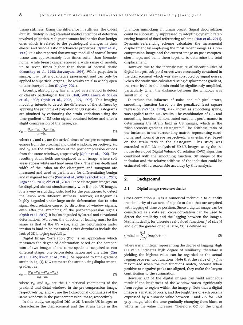
slight compression of the tissue, i.e.

e11 ¼ðt1b�t1aÞ�ðt2b�t2aÞ

t1b�t1að1Þ

where t1a and t1b are the arrival times of the pre-compression

echoes from the proximal and distal windows, respectively; t2a

and t2b are the arrival times of the post-compression echoes

from the same windows, respectively (Ophir et al., 1996). The

resulting strain fields are displayed as an image, where soft

areas appear white and hard areas black. The mean depth and

width of the lesion on the elastogram and sonogram are

measured and used as parameters for differentiating benign

and malignant lesions (Kumar et al., 2009; Lyshchik et al., 2005;

Rago et al., 2007; Zhi et al., 2007). Since elastogram images can

be displayed almost simultaneously with B-mode US images,

it is a very useful diagnostic tool for the practitioner to detect

the lesion with different stiffness. However, elastogram is

highly degraded under large strain deformation due to echo

signal decorrelation caused by distortion of window signals,

even after the stretching of the post-compression signals

(Ophir et al., 2002). It is also degraded by lateral and elevational

deformations. Moreover, the direction of loading must be the

same as that of the US wave, and the deformation under

tension is hard to be measured. Other drawbacks include the

lack of 3D imaging capability.

Digital Image Correlation (DIC) is an application which

measures the degree of deformation based on the compar-

ison of two images of the same specimen acquired at two

different stages: one before deformation and one after (Chu

et al., 1985; Kwon et al., 2010). As opposed to time-gradient

strain in Eq. (1), DIC estimates the strain using displacement-

gradient as

e11 ¼ðx1b�x1aÞ�ðx2b�x2aÞ

x1b�x1að2Þ

where x1a and x1b are the 1-directional coordinates of the

proximal and distal windows in the pre-compression image,

respectively; x2a and x2b are the 1-directional coordinates of the

same windows in the post-compression image, respectively.

In this study, we applied DIC to 2D B-mode US images to

characterize the displacement and the strain fields in the

phantom mimicking a human breast. Signal decorrelation

could be successfully suppressed by adopting dynamic refer-

encing instead of fixed referencing scheme (Han et al., 2011).

Dynamic referencing scheme calculates the incremental

displacement by employing the most recent image as a pre-

compression image and the current image as post-compres-

sion image, and sums them together to determine the total

displacement.

However, due to the intrinsic nature of discontinuities of

digital images, sub-pixel errors were necessarily contained in

the displacement which was also corrupted by signal noises.

When the strain was calculated using displacement gradient,

the error level in the strain could be significantly amplified,

particularly when the distance between the windows was

small in Eq. (2).

To reduce the influence of noise and sub-pixel errors,

smoothing function based on the penalized least square

regression (Wahba, 1990), also known as smoothing spline,

was applied to the DIC results. The combination of DIC and

smoothing function demonstrated excellent performance in

determining the strain field in US images, which is the

‘‘displacement-gradient elastogram.’’ The stiffness ratio of

the inclusion to the surrounding matrix, representing carci-

noma and normal tissue respectively, was estimated based

on the strain ratio in the elastogram. This study was

extended to full 3D analysis of 3D US images using the in-

house developed Digital Volume Correlation (DVC) algorithm

combined with the smoothing function. 3D shape of the

inclusion and the relative stiffness of the inclusion could be

estimated with a reasonable accuracy by this analysis.

2. Background

2.1. Digital image cross-correlation

Cross-correlation (CC) is a numerical technique to quantify

the similarity of two sets of signals or data that are acquired

with lagging of time or position. Since a digital image can be

considered as a data set, cross-correlation can be used to

detect the similarity and the lagging between the images.

Mathematically, for discrete real-valued functions f of size N

and g of the greater or equal size, CC is defined as:

ðfUgÞðnÞ �XN�1

m ¼ 0

f ðmÞgðnþmÞ ð3Þ

where n is an integer representing the degree of lagging. High

CC value indicates high degree of similarity; therefore n

yielding the highest value can be regarded as the actual

lagging between two functions. Note that the value of (f . g) is

maximized when the two functions match, because when

positive or negative peaks are aligned, they make the largest

contribution to the summation.

However, CC of the digital images can yield erroneous

result if the brightness of the window varies significantly

from region to region within the image g. Note that a digital

image is a matrix of pixels, and the brightness of each pixel is

expressed by a numeric value between 0 and 255 for 8-bit

gray image, with the tone gradually changing from black to

white as the value increases. Therefore, CC for the bright

j o u r n a l o f t h e m e c h a n i c a l b e h a v i o r o f b i o m e d i c a l m a t e r i a l s 1 4 ( 2 0 1 2 ) 7 – 1 8 9

region in the image g can be higher than that for the exactly

matching location with f in dark region. For the balanced

consideration of bright and dark regions, Eq. (3) can be

modified by subtracting the average value from each function

before performing correlation, and normalized to have the

value between 0 and 1 as:PN�1m ¼ 0ðf ðmÞ�f aveÞðgðnþmÞ�gavenÞPN�1

m ¼ 0 ðf ðmÞ�f aveÞ2

n o PN�1m ¼ 0 ðgðnþmÞ�gavenÞ

2n i0:5

� ð4Þ

This is called the normalized cross correlation (NCC) which

yields a value of 1 when two data sets are exactly matched

and values close to 0 when no match is made.

However, computation load for NCC is much heavier than

that for CC, since convolution theorem that allows the use of

Fast Fourier Transforms (FFTs) in Eq. (3) cannot be employed

for Eq. (4). The load can be relieved by adopting the sum table

suggested by Lewis (1995). Sum table is the pre-calculated

look-up table over the whole region of function g, and is

referred to whenever a local sum is calculated. NCC adopting

the sum-table method is called the fast normalized cross-

correlation (FNCC).

FNCC algorithm can be extended to multidimensional data

such as 2D and 3D digital images. When the deformation of

the material is small enough to ignore the local distortion of

the visual pattern of the material, one can assign sub-images

of the material before and after deformation around a point

of interest to functions f and g, respectively, and find the 2D

or 3D dimensional lagging which corresponds to 2D or 3D

displacement of the point (Han et al., 2011). By repeating this

procedure to uniformly distributed grid points, displacement

field can be generated. Furthermore, infinitesimal strain

tensor fields can also be determined by taking the gradient

of the displacement field as

eij ¼12

@ui

@xjþ@uj

@xi

!ð5Þ

where xi, ui, and eij refer to coordinate system vector, dis-

placement vector, and strain tensor, respectively.

DIC algorithms have been mainly developed for 2D images

with 2D matrix data sets. For example, in-plane strains in soft

bio-gel were measured by DIC as a non-contact optical sensor

(Kwon et al., 2010). Zhang and Arola (2004) applied DIC to

biological tissues and biomaterials such as arterial tissues,

bovine hoof horn and total hip replacement. DIC has also

been applied to 3D images such as MRI or CT. Lee et al. (2010b)

created 3D finite element model (FEM) of the breast and

employed 3D NCC to compare localized mismatches between

FEM and clinical MR images. Verhulp et al. (2004) applied 3D

DIC to computed tomography (CT) images to measure the

strain in trabecular bone. However, to the best of our knowl-

edge, the application of DIC to 3D US image has not been

reported to date.

For 3D US image analysis, we developed digital volume

correlation (DVC) algorithm by extending FNCC to 3D to

correlate 3D images composed of multiple 2D image stacks.

In both DIC and DVC algorithms, predetermined multiple

material points were tracked to estimate the variations of

displacement and strain fields with the progress of

deformation.

2.2. Data smoothing

Since digital images are composed of pixels, the accuracy of

cross-correlation is limited to the size of a pixel; thus the

estimated displacements necessarily contain sub-pixel scale

errors. On the other hand, US images are usually corrupted by

signal noises in its acquisition and transmission. The major

source of the noise is the speckle noise generated by small

particles in the solution or liquid which reflect ultrasonic

waves (Bilgen and Insana, 1997). Various approaches for noise

reduction have been proposed (Sanches et al., 2008; Sudha

et al., 2009), but none of them can completely remove the

noise. When DIC is applied to noised US images, the sub-pixel

errors are amplified by signal noise and as a consequence the

displacement field yielded by DIC frequently contains sig-

nificant amount of errors. Since displacement gradients are

used to calculate strains, strains are very sensitive to the

displacement errors particularly when the distances between

the grid points are small. Tracking multiple points usually

involves highly dense grid arrays, and rough strains are

frequently generated even from a reasonably smooth displa-

cement dataset in US images.

To resolve this problem, we adopted a smoothing function

that can significantly reduce the small scale errors (Garcia,

2010). In data analysis, smoothing function intends to reduce

experimental noises while preserving the most important

imprints of a dataset, by eliminating random error ei from

noised dataset yi

yi ¼ yi þ ei ð6Þ

to find a smooth true dataset yi.

The smoothing function employed in this study is based on

the penalized least square regression method (Wahba, 1990)

that minimizes criterion function F as:

minfFðyÞg ¼minXn

i ¼ 1

ðyi�yiÞ2þ sPðyÞ

( )ð7Þ

where the first term in the right-hand side is the data

measured by the residual sum of squares (RSS) and s is a

real positive smoothing parameter that controls the degree of

smoothing. A penalty term P(y) is the roughness of smooth

data and can be expressed as a second-order divided differ-

ence (Weinert, 2007) as

PðyÞ ¼ :Dy:2ð8Þ

where J J denotes the Euclidean norm and D is a tri-diagonal

square matrix, which for the equally spaced data is given as

D¼

�1 1

1 �2 1

& & &

1 �2 1

1 �1

0BBBBBB@

1CCCCCCA

ð9Þ

Minimizing FðyÞ using Eqs. (7) and (8) yields the following

linear system that allows the determination of smoothed

data

y¼ ðIn þ sDTDÞ�1y ð10Þ

where In is n by n identity matrix and DT the transpose of D. In

Eq. (10), it is important to choose an appropriate smoothing

Fig. 1 – Schematics of phantom fabrication procedure and

2D US test setup: (a) Solution containing 5% gelatin was

poured into the mold in half; (b) Once the temperature

dropped to 35 1C the prepared inclusion containing 20%

gelatin was placed on top of it; (c) The solution was poured

to fill the rest of the mold; (d) In 2D US test, the phantom

was uniaxially compressed while the US probe acquired US


parameter s to avoid over- or under- smoothing. It can be

optimally estimated by the method of generalized cross

validation (GCV) introduced by Wahba (1990). When D is

given as in Eq. (9), the GCV method selects the parameters

that minimizes the GCV score given by

GCVðsÞ �nPn

i ¼ 11

1þsl2i

�1� �2

DCT2i ðyÞ

n�Pn

i ¼ 11

1þsl2i

� �2ð11Þ

where (l2i )i¼1,2yn are the eigenvalues of DTD and DCT denotes

n-by-n type-2 discrete cosine transform (Strang, 1999). Using

an s value that minimizes the GCV score of Eq. (11), smoothed

data y can be determined. This method allows fast automatic

smoothing of data in multiple dimensions. We adopted this

method to generate smooth displacement and strain fields

without subjective intervention from users.
images of the deformed phantom.
3. Materials and methods

3.1. Numerical validation of DIC smoothing

To validate the performance of the smoothing function in

reducing the roughness of DIC results caused by sub-pixel

errors and signal noises, a digital image of 2000 by 2000 pixels

with random gray values was generated. While the image

was numerically stretched to 10% by 1% increment, evenly

distributed 39�39 grid points across the image were tracked

by the DIC to determine the displacement field at each strain

increment. Strain field was generated from displacement

field by employing the following smoothing schemes: (i) no

smoothing, (ii) strain smoothing, (iii) displacement smooth-

ing, and (iv) combined smoothing. In (ii), smoothing was

applied to the strain field which was generated from the

unsmoothed displacement field, while in (iii) displacement

field was smoothed first, and then strain field was generated

from the smoothed displacement. In (iv), smoothing was

applied to the strain field determined by (iii).

3.2. Phantom preparation

Gelatin based phantoms were designed to contain an inclu-

sion with higher stiffness than the surrounding matrix,

mimicking a carcinoma in a normal tissue. Following the

protocol in Madsen et al. (1982), the inclusion and the matrix

were made with the same constituents to have the similar

echogenicity, i.e., 1 wt% agarose (J.T. Baker, NJ, USA), 2 wt%

glutaraldehide (Sigma-Aldrich, MO, USA), 5 wt% n-propanol

(Fisher-Scientific, NJ, USA), gelatin (Fluka, Germany) (20 wt%

and 5 wt% for inclusion and matrix, respectively), and dis-

tilled water (the remaining wt%). Glutaraldehide acted as a

cross-linker resulting in a melting point of the materials in

the phantom in excess of 68 1C and n-propanol promoted

dissolving of materials. In addition, n-propanol and glutar-

aldehide served as preservatives.

To fabricate the phantom, an inclusion was made first.

After water was heated up to 85 1C, agarose, gelatin, and n-

propanol were added in order. After 3 min of solution time,

glutaraldehide was added, and the solution was kept at an

elevated temperature for 4 more minutes. The resulting

solution was suctioned into a 3 ml syringe (inner diameter

of 8.6 mm) and kept at room temperature for 48 h for gela-

tion. Then, the resulting gel was taken out and stored in

water to prevent shrinkage and dehydration.

Following the same procedure, the solution with 5 wt%

gelatin content was prepared and poured into a long cylind-

rical mold (diameter of 4 cm and height of 8 cm) in half

(Fig. 1(a)). When temperature decreased to 35 1C, the prepared

inclusion was placed on top of the solution and gelled for

5 min (Fig. 1(b)). Then, the solution with 5 wt% gelatin was

added up to the top of the mold and kept 48 more hours

(Fig. 1(c)).

To measure the mechanical properties of the inclusion and

the matrix, cylindrical samples with aspect ratio of 1 (height

and diameter 4 cm each) were additionally made at each

formula following the same procedures.

3.3. Simple compression test

Simple compression tests were conducted using a TA mate-

rial testing machine (TA.xt Plus, Stable Micro Systems, UK)

with a 50 N load cell. Each sample was loaded up to the

engineering strain of 10% at the speed of 10 mm/s. Five tests

were performed at each concentration using different sam-

ples and the results were averaged.

3.4. 2-Dimensional test

The phantom was uniaxially compressed to reach 10%

nominal strain. At each 1% strain step, US image was

recorded using the commercial medical US image machine

(Accuvix XQ, Medison, Korea). US probe was placed in the

direction perpendicular to the axis of cylindrical inclusion so

that circular cross-section of the inclusion was imaged

(Fig. 1(d)). The obtained image has the size of 470�440 pixels

with space resolution of 81 mm/pixel. From the undeformed

image, multiple points were selected at every 20 pixels in

both x and y directions and FNCC algorithm implemented

with sub-pixel algorithm was applied to track these points

through the deformed images. To avoid the decorrelation

errors, dynamic referencing was employed (Han et al., 2011).


Based on the acquired relative movements of grid points,

displacement and strain fields were estimated.

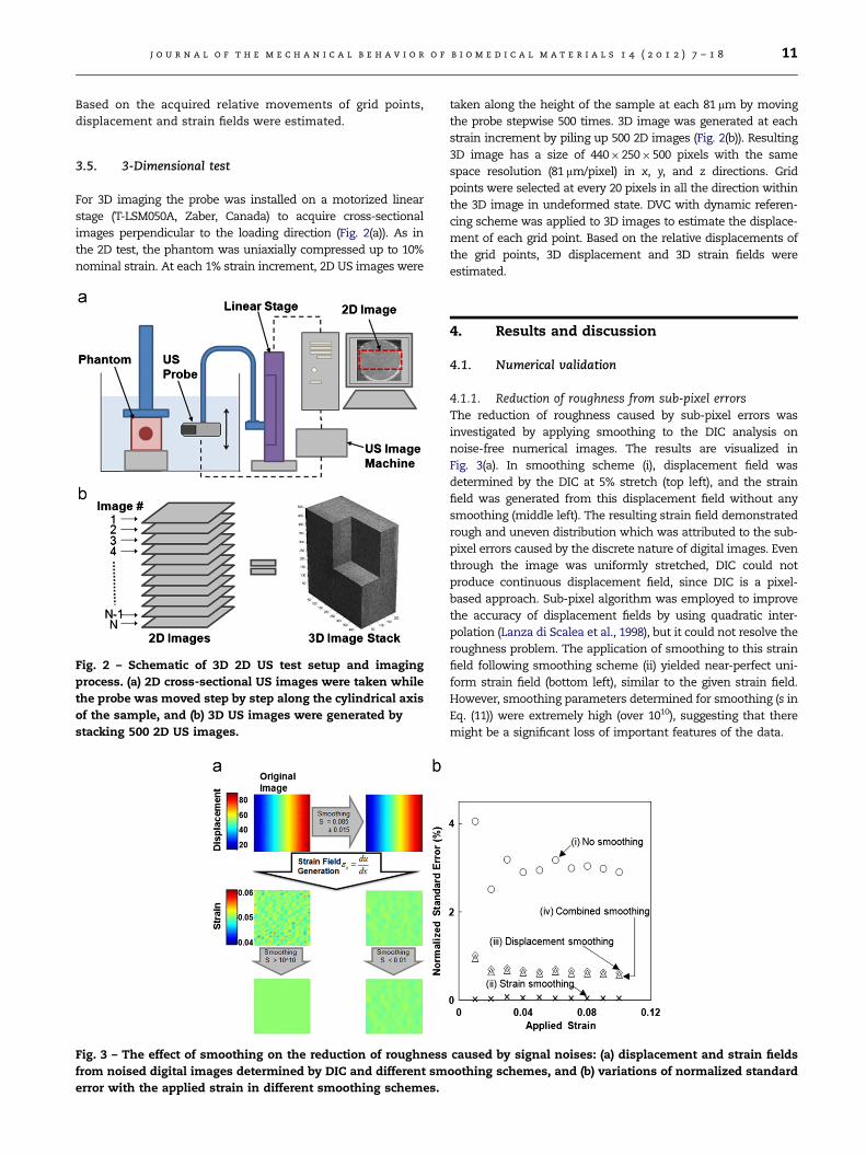
3.5. 3-Dimensional test

For 3D imaging the probe was installed on a motorized linear

stage (T-LSM050A, Zaber, Canada) to acquire cross-sectional

images perpendicular to the loading direction (Fig. 2(a)). As in

the 2D test, the phantom was uniaxially compressed up to 10%

nominal strain. At each 1% strain increment, 2D US images were

Fig. 2 – Schematic of 3D 2D US test setup and imaging

process. (a) 2D cross-sectional US images were taken while

the probe was moved step by step along the cylindrical axis

of the sample, and (b) 3D US images were generated by

stacking 500 2D US images.

Fig. 3 – The effect of smoothing on the reduction of roughness

from noised digital images determined by DIC and different sm

error with the applied strain in different smoothing schemes.

taken along the height of the sample at each 81 mm by moving

the probe stepwise 500 times. 3D image was generated at each

strain increment by piling up 500 2D images (Fig. 2(b)). Resulting

3D image has a size of 440�250�500 pixels with the same

space resolution (81 mm/pixel) in x, y, and z directions. Grid

points were selected at every 20 pixels in all the direction within

the 3D image in undeformed state. DVC with dynamic referen-

cing scheme was applied to 3D images to estimate the displace-

ment of each grid point. Based on the relative displacements of

the grid points, 3D displacement and 3D strain fields were

estimated.

4. Results and discussion

4.1. Numerical validation

4.1.1. Reduction of roughness from sub-pixel errorsThe reduction of roughness caused by sub-pixel errors was

investigated by applying smoothing to the DIC analysis on

noise-free numerical images. The results are visualized in

Fig. 3(a). In smoothing scheme (i), displacement field was

determined by the DIC at 5% stretch (top left), and the strain

field was generated from this displacement field without any

smoothing (middle left). The resulting strain field demonstrated

rough and uneven distribution which was attributed to the sub-

pixel errors caused by the discrete nature of digital images. Even

through the image was uniformly stretched, DIC could not

produce continuous displacement field, since DIC is a pixel-

based approach. Sub-pixel algorithm was employed to improve

the accuracy of displacement fields by using quadratic inter-

polation (Lanza di Scalea et al., 1998), but it could not resolve the

roughness problem. The application of smoothing to this strain

field following smoothing scheme (ii) yielded near-perfect uni-

form strain field (bottom left), similar to the given strain field.

However, smoothing parameters determined for smoothing (s in

Eq. (11)) were extremely high (over 1010), suggesting that there

might be a significant loss of important features of the data.

caused by signal noises: (a) displacement and strain fields

oothing schemes, and (b) variations of normalized standard


In smoothing scheme (iii), displacement field was

smoothed first (top right in Fig. 3(a)), then the strain field

was generated from this displacement field (middle right).

Even though the effect of smoothing was almost invisible in

displacement field and the smoothing parameter s used for

displacement smoothing was very small (0.08570.015), the

strain field determined from this displacement field was

much more uniform than that from scheme (i). This suggests

that this smoothing scheme could effectively reduce the

small level of sub-pixel errors within the displacement field,

which greatly improved the roughness of strains while pre-

serving the main imprint of the original displacement data.

Application of smoothing to this strain field following

scheme (iv) slightly improved the quality of the strain field

with very small smoothing parameter of less than 0.01.

For the quantitative comparison of smoothing schemes,

standard error was normalized by the applied strain as

Errorð%Þ ¼

ffiffiffiffiffiffiffiffiffiffiffiffiffiffiffiffiffiffiffiffiffiffiffiffiffiffiffiffiffiffiffiffiffiffiffiffiffiffiffiPni ¼ 1 ðei�eappliedÞ

2

n

s�

100eapplied

ð12Þ

where n is the number of grid point, ei the measured strain at

i-th grid point, and eapplied the applied strain at each strain

increment.

The variation of normalized standard error with the increase

of strain was plotted for each smoothing scheme in Fig. 3(b). As

visualized in Fig. 3(a), scheme (iii) could decrease the error level

considerably compared to unsmoothed strain field. Scheme (iv)

reduced the error level even further, although the amount of

reduction was not significant. The error level from scheme (ii)

showed the lowest value; however, extremely high degree of

smoothing might have caused the loss of important feature and

the distortion of data. Therefore, considering both error level

and degree of smoothing, scheme (iv) (combined smoothing)

should be the most appropriate smoothing method to reduce

the roughness caused by sub-pixel errors.

4.1.2. Reduction of roughness from signal noisesTo investigate the effect of smoothing on the roughness

caused by signal noises, noises were manually introduced

to the numerical image. It was assumed that two kinds of

Fig. 4 – Schematic of the numerical imagi

noises exist: static and dynamic noises. Static noise repre-

sented noises that might originate from the reflection of

signal from some static components and did not change with

the degree of deformation. Dynamic noise was due to the

floating speckles in the liquid and varied randomly. As an

extreme case, noised images were formed by adding static

and dynamic noises to the original image, with ratio of 25%,

25% and 50% respectively. This image production process is

illustrated in Fig. 4. DIC was performed to the resulting

noised images and the results were smoothed following the

smoothing schemes in the previous section.

The results from the four smoothing schemes are shown in

Fig. 5(a) and (b). Apparently, noises disturbed the tracking

process of DIC and increased the roughness and the error level

in strain field. Compared to the standard errors in the strain

field without smoothing from noise-free images in Fig. 3(b),

those from noised images in Fig. 5(b) were much higher,

indicating that sub-pixel errors were amplified by signal

noises. This was particularly notable in small strain range

where standard errors were extremely high for unsmoothed

data. Since the displacement difference (DL) between adjacent

grid points was very small in this range (e.g. DL was less than

one pixel at 1% strain), strain was highly sensitive to noises.

On the other hand, the standard errors for noised image

after smoothing scheme (iii) did not show much variation

with the strain. Moreover, they were almost in the same

range as those for non-noised image in Fig. 3(b). This

indicates that by applying smoothing to the displacement

field, strain roughness caused by noises could be successfully

suppressed and the quality of strain fields could be signifi-

cantly improved. The result was further enhanced by

smoothing the strain fields from smoothed displacement

field (smoothing scheme (iv)) as illustrated by the insert in

Fig. 5(b). Again, the degree of smoothing in (ii) was extremely

high that the important information of data could be missed

or distorted; thus this scheme should not be suitable, parti-

cularly for the images with nonuniform strain field.

From the above simulation results, it was concluded that

(iv) combined smoothing should be the optimal smoothing

method that can be applied to DIC analysis to reduce the

roughness from both sub-pixel errors and signal noises.

ng process to produce noised images.

Fig. 5 – Effect of smoothing on the reduction of roughness caused by sub-pixel errors: (a) displacement and strain fields in

noise-free images determined by DIC and different smoothing schemes, and (b) variations of normalized standard error with

the applied strain in different smoothing schemes.

Fig. 6 – Engineering stress–strain curves for 20% (solid line)

and 5% (dotted) gelatin samples from simple compression

tests.


4.2. Loading modulus

Representative engineering stress–strain curves from the

simple compression tests were shown in Fig. 6. Viscoelastic

behavior was demonstrated by the significant hysteresis

loops formed by loading and unloading curves in Fig. 6,

especially for 20% gelatin sample. Viscoelasticity is common

to many biological materials; thus, particular attention is

required in investigating the mechanical properties. In this

study, however, only loading curve was considered to avoid

complexity, since unloading did not occur in any of the tests

performed in this study. Note that loading curve might be

varied by the

Loading curves were regarded as linear with R squared

value of 0.9971 and 0.9849, for 20% and 5% gelatin content

samples, respectively. Loading modulus was determined to be

4772 kPa and 971 kPa for each content.

4.3. Displacement-gradient elastogram

2D displacement field and displacement-gradient elastogram

estimated by DIC at 1%, 5%, and 10% compressive strains are

presented with B-mode US image in Fig. 7. The existence of

inclusion can be recognized from both the displacement field

and the elastogram at each strain. Note that the displace-

ment fields are relatively smooth across the images at all

strains; however, elastograms derived from displacement

fields show highly rough and discontinuous strain distribu-

tions. This is because of the intrinsic sensitivity of strain

(displacement gradient) to noises and sub-pixel errors. The

roughness of strain field does not allow the accurate estima-

tion of the size and the stiffness of the inclusion.

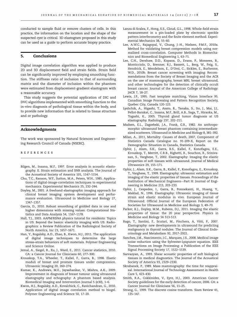
Qualities of the elastograms could be improved by applying

smoothing algorithm to the DIC results, following the three

schemes in Section 3.1, i.e., strain smoothing, displacement

smoothing, and combined smoothing. The resulting elasto-

grams are shown in Fig. 8 with those without smoothing in

the first column. Roughness of strain field was significantly

reduced by all three schemes. Smoothed elastograms show

reasonably smooth strain fields and the circular-shaped low

strain region in the center can be clearly identified. Qualita-

tive comparison with the original shape of the inclusion

indicates that combined smoothing yielded the most satis-

factory result, as suggested by the numerical simulation in

Section 4.1.

By applying DVC to 3D US images, 3D displacement field

and 3D elastograms were produced. The results at 5% com-

pressive strain are presented in Fig. 9 3D images were

sectioned to better illustrate the internal state.

3D displacement field in Fig. 9(a) seems to be smoother

than 2D displacement field in Fig. 7. This is because DVC

considers all three directional displacements, while DIC

ignores the out-of-plane displacement; thus continuity of

the displacement field could be better maintained in 3D

displacement field. Slight distortion of the displacement field

in the central region suggests the existence of the inclusion;

however, the size or the modulus could not be estimated

from this image. The inclusion can be clearly recognized in

3D elastograms that were derived using 3D displacement

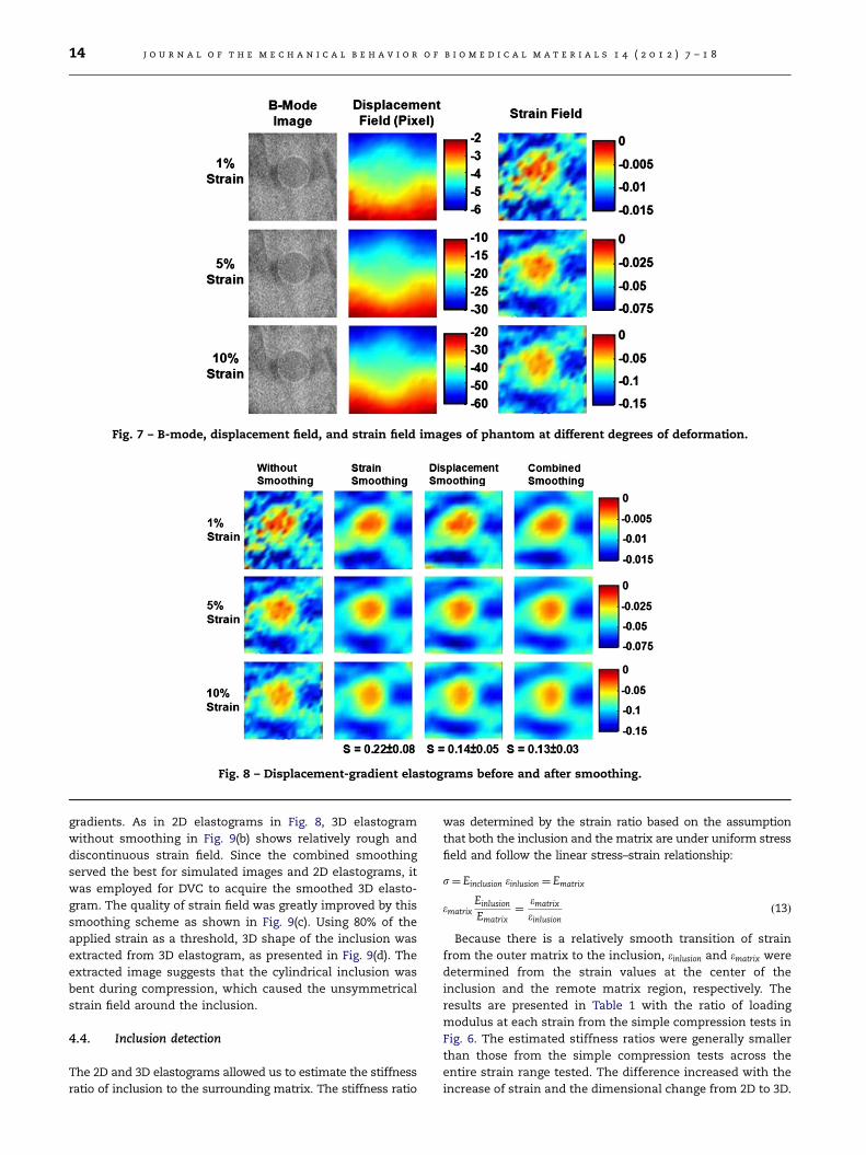
Fig. 7 – B-mode, displacement field, and strain field images of phantom at different degrees of deformation.

Fig. 8 – Displacement-gradient elastograms before and after smoothing.


gradients. As in 2D elastograms in Fig. 8, 3D elastogram

without smoothing in Fig. 9(b) shows relatively rough and

discontinuous strain field. Since the combined smoothing

served the best for simulated images and 2D elastograms, it

was employed for DVC to acquire the smoothed 3D elasto-

gram. The quality of strain field was greatly improved by this

smoothing scheme as shown in Fig. 9(c). Using 80% of the

applied strain as a threshold, 3D shape of the inclusion was

extracted from 3D elastogram, as presented in Fig. 9(d). The

extracted image suggests that the cylindrical inclusion was

bent during compression, which caused the unsymmetrical

strain field around the inclusion.

4.4. Inclusion detection

The 2D and 3D elastograms allowed us to estimate the stiffness

ratio of inclusion to the surrounding matrix. The stiffness ratio

was determined by the strain ratio based on the assumption

that both the inclusion and the matrix are under uniform stress

field and follow the linear stress–strain relationship:

s¼ Einclusion einlusion ¼ Ematrix

ematrixEinlusion

Ematrix¼

ematrix

einlusionð13Þ

Because there is a relatively smooth transition of strain

from the outer matrix to the inclusion, einlusion and ematrix were

determined from the strain values at the center of the

inclusion and the remote matrix region, respectively. The

results are presented in Table 1 with the ratio of loading

modulus at each strain from the simple compression tests in

Fig. 6. The estimated stiffness ratios were generally smaller

than those from the simple compression tests across the

entire strain range tested. The difference increased with the

increase of strain and the dimensional change from 2D to 3D.

Fig. 9 – (a) 3D displacement field, (b) 3D strain field without smoothing, (c) 3D strain field after combined smoothing, and

(d) extracted inclusion shape.

Table 1 – Relative stiffness of inclusion to the matrixestimated from elastograms.

Stiffness ratio (Einclusion/Ematrix)

Strain (%) 2D 3D Simple compression

1 3.4 2.4 5.0

5 3.1 2.2 4.8

10 2.7 2.0 4.7

Table 2 – Diameter of inclusion estimated fromelastograms.

Inclusion diameter (mm)

Threshold 80% 50% Actual

Strain (%) 2D 3D 2D 3D

1 8.8 6.8 9.2 8.2 8.6

5 7.2 5.3 8.8 7.5

10 7.2 5.2 8.8 7.4


The difference may be caused by multiple factors such as

pulling boundary condition on the inclusion, over-smoothing,

and gelatin diffusion. To estimate the stiffness ratio, the strain

at the center of the inclusion and that of the matrix in the

remote region were compared, based on the assumption they

were the under same stress state. However, since the boundary

of the inclusion was bonded to the matrix which was much

more compliant, larger deformation in the matrix developed

the downward pulling force exerted on the boundaries of the

inclusion. As a result, the deformation in the inclusion was

larger than that in free boundary condition; thus the measured

modulus was smaller than that from simple compression test.

This is the opposite stress state to the plane strain condition

with fixed boundaries which yields higher apparent modulus

than that of plane stress condition with free boundaries.

The difference of gelatin content in the inclusion and the

matrix might have caused gelatin diffusion during fabrication

and the ensuing storage process. When the phantom was

fabricated, the gelled inclusion containing 20 wt% gelatin was

placed into matrix solution with 5 wt% gelatin content. Due

to the difference in the contents, gelatin diffusion might

happen during the gelation of the matrix, from the inclusion

to the matrix, resulting in the decrease of inclusion stiffness.

Also, smoothing of strain fields might lessen the contrast

between hard and soft materials, in addition to the intended

reduction of the roughness in the strain fields.

Diameters of the inclusion estimated by using 80% and 50%

of the applied strain as thresholds were presented in Table 2.

Note that inclusion size was varied by the threshold value,

with larger diameter by lower threshold value. When 50% of

the applied strain was employed as a threshold, most

accurate inclusion size was obtained. Similar to stiffness

ratios, estimated inclusion size in 3D was generally smaller

than that in 2D at all strains.

4.5. Inclusion size overestimation

Ophir et al. (1996) reported that the size of the tumor

determined by elastogram was significantly larger than that

by sonogram, only when the tumors are carcinomas. They

hypothesized that since carcinomas elicited a desmoplastic

reaction in the surrounding normal tissue, the size


overestimation might be due to the desmoplasia, which

causes hardening of the normal tissues around the cancer.

Size overestimation due to desmoplasia was mimicked by

varying the boundary layer formed by gelatin diffusion during

phantom fabrication process in Fig. 1(c). Gelatin diffusion was

promoted by increasing the surface-to-volume ratio, which

could be achieved by decreasing the inclusion size and

changing the inclusion shape from circular to non-circular.

For this, cylindrical inclusion prepared by the protocols

described in Section 3.2 was cut into a half-cylindrical and

a quarter-cylindrical shape. Surface-to-volume ratio of a full-,

a half-, and a quarter-cylindrical inclusion was 2/r, and (2þ4/

p)/r and (2þ8/p)/r, i.e., 0.23 mm�1, 0.38 mm�1 and 0.53 mm�1,

respectively. Phantoms were made using these inclusions

and their 2D elastograms were created by applying combined

smoothing. Post-destructive investigation qualitatively con-

firmed that the ratio of boundary layer to entire volume was

relatively proportional to surface-to-volume ratio.

B-mode US and elastogram images of the phantoms con-

taining different inclusions are illustrated in Fig. 10. The

position of the inclusion obtained from B-mode images is

indicated in the elastogram by solid black lines. Comparisons

between the elastograms with different inclusions suggest

that as the size of inclusion was decreased, the contrast

between the inclusion and the matrix became indistinct. This

is quantified in Table 3 which presents the decrease of

stiffness ratio with the decrease of size of inclusion. In a

quarter-cylindrical inclusion, almost the entire volume was

affected by diffusion; therefore, strain difference between the

inclusion and the matrix was much smaller than that in an

inclusion with a lower surface-to-volume ratio. The shape of

the inclusion was also blurred, resulting in the over-estimation

Fig. 10 – B-mode images and elastograms of a fu

Table 3 – Relative stiffness of various inclusions to the matrix

Stiffness ratio (Einclusion/Ematrix)

Inclusion (%) Full cylinder Half cylinder

1 3.4 2.8

5 3.1 2.5

10 2.7 2.4

of inclusion size in the elastogram. These results suggest that

as the bonding between the inclusion and the matrix such as

boundary layer or desmoplasia increases, the shape of the

inclusion becomes less vivid and the size of the inclusion tends

to be overestimated in the elstogram, which is consistent with

the report by Ophir et al. (1996).

4.6. Applications

Usually, malignant tumors are harder than benign tissues

(Ophir et al., 1999) and therefore time-gradient elastograms

have been frequently used to detect carcinomas (Krouskop

et al., 1998; Parker et al., 2011). However, because of relatively

poor resolution of conventional time-gradient elastograms,

the application has been limited to qualitative diagnosis of

diseased lesion, even though it has the advantage of real time

imaging capability. The displacement-gradient elastogram

proposed in this study has more flexibility in employing

reference schemes (dynamic or fixed referencing) and

smoothing function; thus it can have better resolution and

can detect the size and the relative modulus of the stiff lesion

with a better accuracy. They can also be applied to acquire 3D

elastograms that can provide information on 3D shape and

3D stiffness variation of the stiff lesion. Currently, the

computation required to acquire displacement-gradient elas-

togram is too intensive to be performed in real-time, but the

rapid growth of computing power may soon make the real-

time processing available. Real-time 3D displacement-gradi-

ent elastogram can be used congruently with other medical

practices such as biopsy. When a suspected cyst is found by

modalities such as mammogram or MRI, biopsy is frequently

ll, a half and a quarter cylindrical inclusions.

from 2D elastograms.

Quarter cylinder Simple compression

2.3 5.0

2.2 4.8

2.1 4.7


conducted to sample fluid or remove clusters of cells. In this

practice, the information on the location and the shape of the

suspected cyst is critical. 3D elastogram proposed in this study

can be used as a guide to perform accurate biopsy practice.

5. Conclusions

Digital image correlation algorithm was applied to produce

2D and 3D displacement field and strain fields. Strain field

can be significantly improved by employing smoothing func-

tion. The stiffness ratio of inclusion to that of surrounding

matrix and the diameter of inclusion within the phantom

were estimated from displacement-gradient elastogram with

a reasonable accuracy.

This study suggests the potential application of DIC and

DVC algorithms implemented with smoothing function to the

in-vivo diagnosis of pathological tissue within the body, and

to provide new information that is related to tissue structure

and or pathology.

Acknowledgments

The work was sponsored by Natural Sciences and Engineer-

ing Research Council of Canada (NSERC).

r e f e r e n c e s

Bilgen, M., Insana, M.F., 1997. Error analysis in acoustic elasto-graphy. II. Strain estimation and SNR analysis. The Journal ofthe Acoustical Society of America 101, 1147–1154.

Chu, T.C., Ranson, W.F., Sutton, M.A., Peters, W.H., 1985. Applica-tions of digital-image-correlation techniques to experimentalmechanics. Experimental Mechanics 25, 232–244.

Doyley, M., 2001. A freehand elastographic imaging approach forclinical breast imaging: system development and perfor-mance evaluation. Ultrasound in Medicine and Biology 27,1347–1357.

Garcia, D., 2010. Robust smoothing of gridded data in one andhigher dimensions with missing values. Computational Sta-tistics and Data Analysis 54, 1167–1178.

Hall, T.J., 2003. AAPM/RSNA physics tutorial for residents: Topicsin US. Beyond the basics: elasticity imaging with US. Radio-graphics: a Review Publication of the Radiological Society ofNorth America, Inc 23, 1657–1671.

Han, Y., Rogalsky, A.D., Zhao, B., Kwon, H.J., 2011. The applicationof digital image techniques to determine the largestress–strain behaviors of soft materials. Polymer Engineeringand Science Online.

Jemal, A., Siegel, R., Xu, J., Ward, E., 2011. Cancer statistics, 2010.CA: a Cancer Journal for Clinicians 60, 277–300.

Krouskop, T.A., Wheeler, T., Kallel, F., Garra, B., 1998. Elasticmoduli of breast and prostate tissues under compression.Ultrasonic Imaging 20, 260–274.

Kumar, K., Andrews, M.E., Jayashankar, V., Mishra, A.K., 2009.Improvement in diagnosis of breast tumour using ultrasoundelastography and echography: A phantom based analysis.Biomedical Imaging and Intervention Journal 5 (e30), 1–6.

Kwon, H.J., Rogalsky, A.D., Kovalchick, C., Ravichandran, G., 2010.Application of digital image correlation method to biogel.Polymer Engineering and Science 50, 17–20.

Lanza di Scalea, F., Hong, S.S., Cloud, G.L., 1998. Whole-field strainmeasurement in a pin-loaded plate by electronic specklepattern interferometry and the finite element method. Experi-mental Mechanics 38, 55–60.

Lee, A.W.C., Rajagopal, V., Chung, J.-H., Nielsen, P.M.F., 2010a.Method for validating breast compression models using nor-malised cross-correlation. Computer Methods in Biomecha-nics and Biomedical Engineering 1, 63–71.

Lee, C.H., Dershaw, D.D., Kopans, D., Evans, P., Monsees, B.,Monticciolo, D., Brenner, R.J., Bassett, L., Berg, W., Feig, S.,Hendrick, E., Mendelson, E., D’Orsi, C., Sickles, E., Burhenne,W.D., 2010b. Breast cancer screening with imaging: Recom-mendations from the Society of Breast Imaging and the ACRon the use of mammography, breast MRI, breast ultrasound,and other technologies for the detection of clinically occultbreast cancer. Journal of the American College of Radiology:JACR 7, 18–27.

Lewis, J.P., 1995. Fast template matching, Vision Interface 95.Canadian Image Processing and Pattern Recognition Society,Quebec City, Canada 120-123.

Lyshchik, A., Higashi, T., Asato, R., Tanaka, S., Ito, J., Mai, J.J.,Pellot-Barakat, C., Insana, M.F., Brill, A.B., Saga, T., Hiraoka, M.,Togashi, K., 2005. Thyroid gland tumor diagnosis at USelastography. Radiology 237, 202–211.

Madsen, E.L., Zagzebski, J.A., Frank, G.R., 1982. An anthropo-morphic ultrasound breast phantom containing intermediate-sized scatterers. Ultrasound in Medicine and Biology 8, 381–392.

Milan, A., 2011, Mortality: Causes of death, 2007, Component ofStatistics Canada Catalogue no. 91-209-X, Report on theDemographic Situation in Canada, Statistics Canada.

Ophir, J., Alam, S.K., Garra, B.S., Kallel, F., Konofagou, E.E.,Krouskop, T., Merritt, C.R.B., Righetti, R., Souchon, R., Sriniva-san, S., Varghese, T., 2002. Elastography: Imaging the elasticproperties of soft tissues with ultrasound. Journal of MedicalUltrasonics 29, 155–171.

Ophir, J., Alam, S.K., Garra, B., Kallel, F., Konofagou, E., Krouskop,T., Varghese, T., 1999. Elastography: ultrasonic estimation andimaging of the elastic properties of tissues. Proceedings of theInstitution of Mechanical Engineers—Part H: Journal of Engi-neering in Medicine 213, 203–233.

Ophir, J., Cespedes, I., Garra, B., Ponnekanti, H., Huang, Y.,Maklad, N., 1996. Elastography: Ultrasonic imaging of tissuestrain and elastic modulus in vivo. European Journal ofUltrasound: Official Journal of the European Federation ofSocieties for Ultrasound in Medicine and Biology 3, 49–70.

Parker, K.J., Doyley, M.M., Rubens, D.J., 2011. Imaging the elasticproperties of tissue: the 20 year perspective. Physics inMedicine and Biology 56 513-513.

Rago, T., Santini, F., Scutari, M., Pinchera, A, Vitti, P., 2007.Elastography: new developments in ultrasound for predictingmalignancy in thyroid nodules. The Journal of Clinical Endo-crinology and Metabolism 92, 2917–2922.

Sanches, J.M., Nascimento, J.C., Marques, J.S., 2008. Medical imagenoise reduction using the Sylvester-Lyapunov equation. IEEETransactions on Image Processing: a Publication of the IEEESignal Processing Society 17, 1522–1539.

Sarvazyan, A., 1993. Shear acoustic properties of soft biologicaltissues in medical diagnostics. The Journal of the AcousticalSociety of America 93, 2329–2330.

Skrabanek, P., 1989. Mass mammography: the time for reapprai-sal. International Journal of Technology Assessment in HealthCare 5, 423–430.

Smith, R.A., Cokkinides, V., Eyre, H.J., 2003. American CancerSociety guidelines for the early detection of cancer, 2006. CA: aCancer Journal for Clinicians 56, 11–25.

Strang, G., 1999. The discrete cosine transform. Siam Review 41,135–147.


Sudha, S., Suresh, G.R., Sukanesh, R., 2009. Speckle Noise reduc-tion in ultrasound images by wavelet thresholding based onweighted variance. International Journal of Computer Theoryand. Engineering 1, 7–12.

Verhulp, E., van Rietbergen, B., Huiskes, R., 2004. A three-dimensionaldigital image correlation technique for strain measurements inmicrostructures. Journal of Biomechanics 37, 1313–1320.

Wahba, G., 1990. Spline Models for Observational Data, CBMS-NSFRegional Conference Series in Applied Mathematics 59, Phila-delphia: SIAM: Society for Industrial and Applied Mathe-matics, pp. 45–65.

Weinert, H.L., 2007. Efficient computation for Whittaker–Henderson smoothing. Computational Statistics and DataAnalysis 52, 959–974.

Zhang, D., Arola, D.D., 2004. Applications of digital image correla-tion to biological tissues. Journal of Biomedical Optics 9,691–699.

Zhi, H., Ou, B., Luo, B.-M., Feng, X., Wen, Y.-L., Yang, H.-Y., 2007.Comparison of ultrasound elastography, mammography, andsonography in the diagnosis of solid breast lesions. Journal ofUltrasound in Medicine: Official Journal of the AmericanInstitute of Ultrasound in Medicine 26, 807–815.

Application of digital image cross-correlation and...

Documents

Transcript of Application of digital image cross-correlation and...