Application of Deep Learning Algorithms for Automated ... · Automated Detection of Arrhythmias...
91
Application of Deep Learning Algorithms for Automated Detection of Arrhythmias with ECG Beats OH SHU LIH SCHOOL OF MECHANICAL AND AEROSPACE ENGINEERING 2019 Deep Learning For Arrhythmias Detection OH SHU LIH 2019
Transcript of Application of Deep Learning Algorithms for Automated ... · Automated Detection of Arrhythmias...

Application of Deep Learning Algorithms for
Automated Detection of Arrhythmias with ECG Beats
OH SHU LIH
SCHOOL OF MECHANICAL AND AEROSPACE ENGINEERING
2019
Deep
Learn
ing
Fo
r Arrh
yth
mias D
etection
O
H S
HU
LIH
2
01
9

Application of Deep Learning Algorithms for
Automated Detection of Arrhythmias with ECG Beats
By
OH SHU LIH
School of Mechanical and Aerospace Engineering
A thesis submitted to the Nanyang Technological University
in partial fulfilment of the requirement for the degree of
Master in Engineering
2019

Statement of Originality
I hereby certify that the work embodied in this thesis is the result of original
research, is free of plagiarised materials, and has not been submitted for a
higher degree to any other University or Institution.
12/03/2019
. . . . . . . . . . . . . . . . . . . . . . . . . . . . . . . . . . . . . . . . . . . .
Date Oh Shu Lih

Supervisor Declaration Statement
I have reviewed the content and presentation style of this thesis and declare
it is free of plagiarism and of sufficient grammatical clarity to be examined.
To the best of my knowledge, the research and writing are those of the
candidate except as acknowledged in the Author Attribution Statement. I
confirm that the investigations were conducted in accord with the ethics
policies and integrity standards of Nanyang Technological University and
that the research data are presented honestly and without prejudice.
12/03/2019
. . . . . . . . . . . . . . . . . . . . . . . . . . . . . . . . . . . . . . . . . . . .
Date Eddie Ng Yin-Kwee, PhD

Authorship Attribution Statement
This thesis contains material from 2 paper(s) published in the following peer-
reviewed journal(s) in which I am listed as an author.
Chapter 6.1.1 is published as Oh, S. L., Ng, E. Y., San Tan, R., & Acharya, U. R.
(2018). Automated diagnosis of arrhythmia using combination of CNN and LSTM
techniques with variable length heart beats. Computers in biology and medicine,
102, 278-287. https://doi.org/10.1016/j.compbiomed.2018.06.002
The contributions of the co-authors are as follows:
• I wrote the drafts of the manuscript. The manuscript was revised together
with A/Prof Ng Yin Kwee, Dr. Rajendra Acharya and Dr. Tan Ru San.
• I co-designed the study with A/Prof Ng Yin Kwee and Dr. Rajendra
Acharya and performed the experimental work at Ngee Ann Polytechnic.
• Dr Tan Ru San assisted in the interpretations of clinical write-up and
discussions.
Chapter 6.1.2 is published as Oh, S. L., Ng, E. Y., San Tan, R., & Acharya, U. R.
(2019). Automated beat-wise arrhythmia diagnosis using modified U-net on
extended electrocardiographic recordings with heterogeneous arrhythmia types.
Computers in biology and medicine, 105, 92-101.
https://doi.org/10.1016/j.compbiomed.2018.12.012
The contributions of the co-authors are as follows:
• I wrote the drafts of the manuscript. The manuscript was revised together
with A/Prof Ng Yin Kwee, Dr. Rajendra Acharya and Dr. Tan Ru San.
• I co-designed the study with A/Prof Ng Yin Kwee and Dr. Rajendra
Acharya and performed the experimental work at Ngee Ann Polytechnic.
• Dr Tan Ru San assisted in the interpretations of clinical write-up and
discussions.

12/03/2019
. . . . . . . . . . . . . . . . . . . . . . . . . . . . . . . . . . . . . . . . . . . .
Date Oh Shu Lih

I
ABSTRACT
Arrhythmia is the anomalies of cardiac conduction system that is characterized by abnormal
heart rythms. Prolong arrhythmias are life threatening and can often lead to other cardiac
diseases. Abnormalities in the conduction system is reflected upon the morphology of the
electrocardiographic (ECG) signal and the assessment of these signal can be extremely
challenging and time-consuming. Morphological features of arrythmias ECG signals are
low in amplitudes and the changes within can sometimes be very subtle. Therefore, the
main aim of this study is to develop an automated computer aided diagnostic (CAD) system
that can potentially expedite the process of arrhythmia diagnosis, which will allow the
clinicians to provide better care and timely intervention for the patient.
In machine learning, the performance of classification largely depends on the quality of
features extracted. Therefore, the process of obtaining useful information which effectively
differentiate the specific classes into groups is crucial. Generally, there are two types of
features used in machine learning, handcrafted features and learned features. Many of the
techniques developed in earlier literature involved the use of handcrafted features. In order
to engineer a handcrafted feature it typically requires one to have extensive domain
knowledge and the latter experimentation cost in selecting the optimal features for a specific
classification model can be costly as well. Learned features on the other hand is obtained
though self-discovery by the artificial intelligence system, it obviates the process of manual
engineering and the current state of the art technique used in obtaining learned feature is
through deep learning.

II
In this research, two different deep learning architectures are tested for diagnosing
arrhythmic ECG signals. The first proposed deep learning architecture is a hybrid neural
network of convolutional layers and long short-term memory (LSTM) units capable of
providing single class prediction for each variable-length data ECG segments. The second
proposed model is U-net ,a fully convolutional auto encoder with skip connections, which
provides a much detailed analysis for the ECGs as each of the detected beats can be marked
with a specific heart conditions.
Both models are trained and tested against the MIT-BIT arrhythmia database. 5 cardiac
conditions, normal sinus rhythm, atrial premature beats (APB), premature ventricular
contraction (PVC), left bundle branch block (LBBB) and right bundle branch block (RBBB)
are segmented from the recordings for evaluation. Additionally, the ten-fold cross
validation strategy has been employed in the project to confirm the robustness of the
proposed models.
Findings of this research will redound in benefiting the ECG screening procedures,
considering that deep learning models are capable of achieving considerable accuracy and
details in categorizing the individual arrhythmias beats with minimal preprocessing applied.
The future work intends to acquire more ECG records to increase the variance of the current
dataset, implementation of generative adversarial network (GAN) for ECG augmentation
and to explore on other cardiac diseases.

III
Keywords: arrhythmias, convolutional neural network, deep learning, electrocardiogram,
long short-term memory, U-net, autoencoder

IV
ACKNOWLEDGEMENT
First and foremost, I would like to express my sincere gratitude to my supervisor Dr. Eddie
Ng Yin Kwee for his guidance and encouragement throughout the course of this project.
Secondly, I am thankful to my boss, Dr. Rajendra Udyavara Acharya, without his
encouragement and understanding, this project would never have been possible.
I would also like to thank my friends and colleagues. Especially, Mr. Muhammad Adam
Bin Abdul Rahim and Mr. Joel Koh En Wei whom have encourage me and made my
learning in Nanyang Technological University (NTU) an enjoyable one.
Last but not least, I wish to express my greatest indebtedness to my family, whom have
given me constant support, love and encouragement throughout the entire course of this
work.

I
Table of Contents
Abstract ................................................................................................................................. I
Acknowledgement ............................................................................................................. IV
List of Figures .................................................................................................................... IV
List of Tables ....................................................................................................................... V
1 Chapter One – Introduction ...........................................................................................1
1.1 Motivations & Scope of Research ......................................................................... 1
1.2 Arrhythmias........................................................................................................... 2
1.3 Aims of Research .................................................................................................. 5
2 Chapter Two – Literature Review .................................................................................6
3 Chapter Three – Cardiac System & Electrocardiogram ..............................................20
3.1 Anatomy & Physiology of Human Heart ............................................................ 20
3.2 Conduction System of the Heart ......................................................................... 21
3.3 Electrocardiogram & Characteristics of Arrhythmic Signals ............................. 23
3.3.1 Bundle Branch Block ............................................................................................... 24
3.3.2 Atrial Premature Beats ............................................................................................ 25
3.3.3 Premature Ventricular Contraction ........................................................................ 26
4 Chapter Four – Deep Neural Network .........................................................................27
4.1 Artificial Neural Network & Deep Network ....................................................... 27
4.1.1 Convolutional Neural Network (CNN) ..................................................................... 29
4.1.2 Recurrent Neural Networks (RNN) and Long short-term memory (LSTM) ............. 31
4.1.3 U-Net ....................................................................................................................... 32

II
5 Chapter Five – Materials & Methodology ...................................................................34
5.1 Data Description .................................................................................................. 34
5.2 Preprocessing ...................................................................................................... 35
5.2.1 Homogeneous segmentation (CNN-LSTM network) .............................................. 35
5.2.2 Heterogeneous segmentation (U-net) .................................................................... 36
5.3 Data normalization and the designs of training target ........................................ 38
5.4 Proposed Network Architectures ........................................................................ 41
5.4.1 CNN-LSTM model .................................................................................................... 41
5.4.2 Modified U-net model ............................................................................................ 43
5.4.3 Convolution layer .................................................................................................... 46
5.4.4 Max pooling ............................................................................................................ 47
5.4.5 Global pooling ......................................................................................................... 47
5.4.6 Long short term memory (LSTM) ............................................................................ 48
5.4.7 Fully connected layer .............................................................................................. 49
5.4.8 Activation function .................................................................................................. 50
5.4.9 Dropout regularization ............................................................................................ 51
5.4.10 Training and evaluation .......................................................................................... 51
6 Chapter Six – Results & Discussion ............................................................................55
6.1 Results ................................................................................................................. 55
6.1.1 CNN-LSTM ............................................................................................................... 55
6.1.2 Modified U-net ........................................................................................................ 58
6.2 Discussion ........................................................................................................... 63
7 Chapter Seven – Conclusion & Future Work ..............................................................66
7.1 Conclusion........................................................................................................... 66

III
7.2 Future Work ........................................................................................................ 68
References ...........................................................................................................................70
Appendix A: Published Papers ...........................................................................................75

IV
LIST OF FIGURES
Figure 1: Cardiovascular system of the human body with two circulatory system:(i)
pulmonary circuit and (ii) systemic circuit. ....................................................................... 20
Figure 2: Heart conduction system (yellow) and distribution of contractile stimulus at
different cardiac cycle phases. ........................................................................................... 22
Figure 3: Typical normal ECG waveform. ........................................................................ 23
Figure 4: Typical characteristics of LBBB ECG beats ..................................................... 24
Figure 5: Typical characteristics of RBBB ECG beats ..................................................... 25
Figure 6: Typical characteristic of APB ECG beats .......................................................... 26
Figure 7: Typical characteristics of PVC ECG beats ........................................................ 26
Figure 8: An analogous representation of biological neuron (A) and artificial neuron (B).
........................................................................................................................................... 27
Figure 9: A schematic representation of a typical U-net structure .................................... 32
Figure 10: Homogeneous ECG arrhythmia segments. ...................................................... 39
Figure 11: Normalized ECG signals that are heterogeneously segmented with annotated R
peaks (N = Normal, L = LBBB, R = RBBB, A = APB, P = PVC) ................................... 40
Figure 12: An illustration of the proposed CNN-LSTM architecture. .............................. 42
Figure 13: An illustration of the modified U-net architecture ........................................... 44
Figure 14: Data distribution of the ECG segments used for training and testing the proposed
networks. ............................................................................................................................ 52
Figure 15: Accuracy plots for the various schemes during CNN-LSTM model training. . 56

V
Figure 16: Scheme A - Confusion matrix of the classified ECG segments (N = Normal, L
= LBBB, R = RBBB, A = APB, P = PVC). ....................................................................... 58
Figure 17: Scheme B - Confusion matrix of the classified ECG segments (N = Normal, L =
LBBB, R = RBBB, A = APB, P = PVC). .......................................................................... 58
Figure 18: Accuracy plots form the multiple classification heads of the U-net model. .... 59
Figure 19: Confusion matrix of the classified ECG beats (N = Normal, L = LBBB, R =
RBBB, A = APB, P = PVC). ............................................................................................. 61
Figure 20: Confusion matrix for R peak prediction ........................................................... 61
Figure 21: Annotated ECG segments (blue) along with the predicted R peaks (red vertical
dotted lines). Below each ECG segment is the corresponding class activation maps
produced by the modified U-net model. The highly activated areas are depicted in red color.
........................................................................................................................................... 62
LIST OF TABLES
Table 1: Automated detection of the arrhythmias using conventional techniques. ............. 7
Table 2: Automated detection of the arrhythmias using deep learning approach. ............ 15
Table 3: Extracted ECG segments and the corresponding sample length ranges. ............. 35
Table 4: Number of ECG segments and their corresponding conditions .......................... 37
Table 5: Total number of ECG beats available for training and testing the U-net ............ 37
Table 6: Detailed overview of the proposed CNN-LSTM model. .................................... 43
Table 7: Detailed overview of the proposed U-net model. ................................................ 45

VI
Table 8: Average performance for the different schemes tested against CNN-LSTM model.
........................................................................................................................................... 57
Table 9: Average performance of the best U-net model across all 10 folds. ..................... 60

1
1 CHAPTER ONE – INTRODUCTION
1.1 MOTIVATIONS & SCOPE OF RESEARCH
Timely and accurate diagnosis of abnormal arrhythmias is crucial in cardiac health
monitoring. Only expert clinicians are however able to provide the necessary guidance and
treatment for the patients, thereby reducing the risk of cardiovascular events and death.
The current medical routine for arrhythmia screening requires careful study of ECGs by
experienced clinicians. This process is mundane and laborious. Additionally, short-term
ECGs taken in clinical settings are insufficient for the doctors to diagnose the activity of
heart comprehensively. Therefore, diagnosis of suspected arrhythmias typically requires
patients to wear a small recorder over their chest for continuous monitoring of heart’s
functioning during the daily activities [1]. Data collected from such devices often last over
a day or two. Hence, it is mentally taxing and visually strenuous for the clinicians to
manually read these long sequence of ECG data. Moreover, there is a high possibility that
small changes in the ECG signal may be left undetected by the human eye. Hence, the
proposed computer-aided diagnosis (CAD) system can be utilized as a tool to help in
eliminating the above said problems of observer variability and reduce the time taken for
ECG diagnosis.

2
1.2 ARRHYTHMIAS
In a 2017 global report, there are 962 million people of age 60 years and above. The United
Nations has projected that the number of elderly is going to be double by 2050 and the
estimated population would be around 2.1 billion. People with 80 years of age and over is
also expected to triple from 2017 to 2050, rising from 137 million to 425 million [2]. Aging
reduces physiological reserve as such the cardiovascular system may start to deteriorate and
lose its function [3]. As a result, elderlies are more prone to develop cardiovascular diseases
[4].
The cardiovascular system undergoes structural and functional changes as one ages. The
blood vessels lose their elasticity and the heart muscle thickens due to excessive loads.
These changes are mainly brought about by the increased apoptosis of the surrounding cells
and the buildup of fibro-lipid plaque on the heart muscles due to myocyte enlargement [5].
Accumulation of fibro fatty tissue impacts the heart function negatively, it causes the
cardiac conduction system to be disrupted leading to arrhythmias along with other cardiac
diseases. Less commonly, arrhythmia can be life threatening due to compromise of
mechanical cardiac output causing sudden deaths. [6-11]. The most common types of
arrhythmias found in older adults are premature beats (APB), premature ventricular
contraction (PVC), left bundle branch block (LBBB) and right bundle branch block (RBBB)
[3].
According to epidemiologic studies conducted over the past three decades, the prevalence
of LBBB generally ranges from 0.1–0.8% and the prognosis of LBBB is commonly

3
associated to the coronary artery disease, hypertension, and cardiomyopathy [12]. In
Framingham [6], according to their 18-years of study, 1.1% of the observed population are
newly diagnosed with LBBB, 27% of which are formerly free from any cardiovascular
abnormalities. In addition, 33% of these healthy with LBBB cases eventually developed the
coronary heart disease. Among the studied population, in less than 10 years upon the onset
of LBBB, 50% died from cardiovascular diseases [6]. In another study, the incidence and
prevalence of LBBB are found to be increasing with age for both men and women and
almost twice in patients with LBBB developed cardiovascular disease as compared to the
controls [7]. All these evidence suggests that LBBB is a strong precursor to cardiovascular
diseases.
Similar to LBBB, the prevalence of RBBB increases with age. In Framingham study, 1.3%
of the studied population developed RBBB over 18-years of follow-up. It is identified that,
the incidence of coronary artery disease in RBBB patients is 2.5 times greater and the
incidence of congestive heart failure is approximately 4 times greater in RBBB patients
compared to the perfectly healthy subjects [13]. In another study, the prevalence of RBBB
is found to increase from 0% to 4.1% for men and 1.6% for women over the age group 30–
39 to 75–79 years old. Higher mortality rate due to heart disease is found in men with RBBB
while women younger than 60 years of age with RBBB is often associated with
hypertension [8].
Premature atrial contractions or APB is frequently seen among elderly. It is observed that
99% of individuals aged 50 years or more have at least one episode of premature atrial

4
contractions during the 24-hour Holter monitoring [14]. The APB plays a critical role in the
pathogenesis of atrial fibrillation (AF). Over the years, several studies have shown strong
association between APB and the increased risk of AF [9, 15, 16]. Subclinical atrial
arrhythmias which include APB have relation to the increased risk of stroke and death [9,
10, 15-17]. Furthermore, a study by Inoue et al [18] reported that the ablation of APB in
contrast to pulmonary vein is responsible for the high recurrence-free survival rate among
patients with chronic AF. This suggests that the causation of AF is likely linked to the
abnormal electrical firings in the atria [18].
According to the various 24-hour ambulatory electrocardiogram (ECG) studies, the
prevalence of PVC were significantly higher among the asymptomatic elderly groups
compared to the younger age groups ranging from approximately 69% to 96% [11, 19, 20].
PVCs are often associated with cardiac diseases with increased risk of sudden death,
however it can also be observed in the absence of identifiable heart disease [21, 22].
Although the resting ECG or exercise stress testing often indicates correct prognosis in
healthy individuals [23]. In patients over 62 years of age with coronary disease having PVC
is indicates the adverse health condition [24]. Furthermore, it was found in Framingham
Heart study that men without any identifiable coronary heart disease and had frequent
ventricular premature beats were in correlation with increased risk of mortality [25].

5
1.3 AIMS OF RESEARCH
The aim of this study is to develop a CAD system for arrhythmias using ECG signals. This
methodology serves as a stepping stone for arrhythmias research in deep learning diagnosis.
The detection of arrhythmias using ECG morphology and rhythm are vital for the
development of CAD system. In the past, preprocessing and extraction of meaningful
features are accomplished through hand coded operations. It typically requires one to have
extensive knowledge to select the appropriate features for the specific classification task.
This research aims to overcome and the reliance on hand-crafted features and applied
preprocessing techniques for ECG diagnosis. Deep learning models are end-to-end system
capable of self-learning and discovery. Additionally, with the appropriate design such
system has the ability to handle variable length data which is suitable for ECG classification.
Potentially, the proposed system is capable of providing rapid and precise diagnosis that
are extremely beneficial in hospitals, polyclinics and community care units. The hypothesis
of this research is that the deep learning algorithms can recognize ECG morphological
differences between arrhythmias accurately.

6
2 CHAPTER TWO – LITERATURE REVIEW
Over the years many automated diagnostic systems have been developed for the arrhythmia
detection using ECG signals from MIT-BIH arrhythmia dataset [26]. Table 1 shows
the summary of published studies on automated detection of arrhythmia using conventional
machine learning techniques. Table 2 shows the summary of published studies using
deep learning techniques. It should be noted that not all arrhythmias used in the studies are
identical.
Conventional machine algorithms often require complex feature engineering and extensive
knowledge of the domain, features need to be carefully selected before it can be the used
for classification. More often than not, dimensionality reduction techniques are applied to
the features for easier processing. It is noticeable that few of these machine learning studies
have used linear features [27-29], nonlinear features [30-36], and wavelet transformed
coefficients [34] for classification.
Yeh et al. [27] applied linear discriminant analysis for classification using only
morphological features extracted from the ECG signals. Difference operation method
(DOM) that comprises of few threshold filters are used in identifying the PQRST
components. Upon identifying the PQRST waves, the morphological features are extracted.
The study obtained an accuracy of 96.23% using just four features. In another
morphological based study, Karimifard et al. [30] have extracted the cumulants from the
ECG beats based on the Hermite model. The method has proved its effectiveness in

7
suppressing the morphological differences whitin classses reducing the effects of time,
amplitude shift and noise.
Martis et al. [37] implemented principal component analysis (PCA) on ECG beats and
achieved an accuracy of 98% for classification. Only a dozen of PCA components are
selected and used for training the least square-support vector machine classifier. Martis et
al. [35] used PCA with higher order statistics (HOS) features to identify the morphological
differences in arrhythmia ECG beats. The same reduction is used by Li et al. [33] to extract
the components from the discrete wavelet transformed (DWT) signals. Their study also
attained 97.3% classification accuracy using various reducion methods employed on the
wavelet transformed ECG. All these conventional machine studies confirm that arrhythmias
are caused by the abnormalies in the cardiac conduction system and are clearly expressed
upon ECG signals. It is therefore evident that the use of CAD system can help in identifying
the transient changes in the ECG and improve the efficacy of arrhythmia detection.
Author,
Year
Extracted
features
Database Analyzed data Classifier Performance
Sahoo et
al., 2017
[29]
ECG
morphology
and heart
rate features
MITDB Normal
LBBB
RBBB
Paced
Total
(109494)
Square-Support
Vector Machine
(SVM)
ACC:
98.39%
SEN:
99.87%
PPV:
99.69%

8
Li et al.,
2016 [28]
beat to beat
interval and
entropies
extracted
from
Wavelet
Packet
Decomposit
ion (WPD)
MITDB Normal
(90082)
Ventricular ectopic
(7009)
Supra-ventricular
ectopic
(2779)
Fusion
(803)
Unknown
(15)
Total
(100688)
Random forest ACC:
94.61%
Elhaj et al.,
2016 [32]
Reduction
of Discrete
Wavelet
coefficients
using
Principal
Components
Analysis
(PCA) and
reduction of
Higher-
Order
MITDB Normal
(90580)
Ventricular ectopic
(7707)
Supra-ventricular
ectopic
(2973)
Unknown
(7050)
Fusion
(1784)
Square-Support
Vector Machine
(SVM with Radial
Basis Function)
ACC:
98.91%
SEN:
98.91%
SPEC:
97.85%

9
Statistics
(HOS)
cumulants
using
Independent
component
analysis
(ICA)
Total
(110094)
Li et al.,
2016 [33]
Reduction
of
Discrete
Wavelet
using
Principal
Components
Analysis
(PCA) and
kernel-
independent
component
analysis
(kernel ICA)
MITDB
Normal
(400)
APB
(200)
PVC
(400)
LBBB
(400)
RBBB
(400)
Total
(1800)
Support Vector
Machine (SVM)
ACC:
98.8%
SEN:
98.50%
SPEC:
99.69%
PPV:
98.91%
Martis et
al ., 2013
[34]
Reduction
of Discrete
wavelet
transform
(DWT) sub
bands using
MITDB Normal
(90580)
Ventricular ectopic
(7707)
Supra-ventricular
ectopic
Probabilistic
Neural Network
(PNN)
ACC:
99.28%
SEN:
97.97%,
SPEC:
99.83%

10
Independent
Component
Analysis
(ICA)
(2973)
Unknown
(7050)
Fusion
(1784)
Total
(110094)
PPV:
99.21%
Martis et
al ., 2013
[35]
Higher-
Order
Bispectrum
and
Principal
Components
Analysis
(PCA)
MITDB
Normal
(10000)
APB
(2544)
PVC
(7126)
LBBB
(8069)
RBBB
(7250)
Total
(34989)
Least Square-
Support Vector
Machine (LS-
SVM with Radial
Basis Function)
ACC:
93.48%,
SEN:
99.27%
SPEC:
98.31%
Martis et
al ., 2012
[37]
Principal
Components
Analysis
(PCA) of
MITDB
Normal
(10000)
APB
(2544)
Least Square-
Support Vector
Machine (LS-
ACC:
98.11%
SEN:
99.90%

11
ECG beat
segments
PVC
(7126)
LBBB
(8069)
RBBB
(7250)
Total
(34989)
SVM with Radial
Basis Function)
SPEC:
99.10%
PPV:
99.61%
Karimifard
et al., 2011
[30]
Hermite
model of the
Higher-
Order
Statistics
(HOS)
MITDB Normal
(2000)
APB
(722)
PVC
(2938)
LBBB
(1456)
RBBB
(2251)
Total
(9367)
1-Nearest
Neighborhood
SPEC:
99.67%
SEN:
98.66%
Martis et
al., 2011
[36]
Higher order
spectra
(HOS)
cumulants
MITDB Normal
(641)
APB and PVC (606)
Support Vector
Machine (SVM
with Radial Basis
Function)
ACC:
98.48%
SEN:
98.90%

12
of Wavelet
packet
decompositi
on (WPD)
Total
(1247)
SPEC:
98.04%
PPV:
98.13%
Yeh et al.,
2009 [27]
Morphologi
cal and heart
rate based
features
MITDB
Normal
(75054)
APB
(2544)
PVC
(7129)
LBBB
(8074)
RBBB
(9259)
Total
(102060)
Linear
Discriminant
Analysis
Accuracy:
96.23%
SENS:
Normal
98.97%
LBBB
91.07%,
RBBB
95.09%
PVC
92.63%
APB
84.68%
Yu et al.,
2008 [38]
time elapse
between R
peaks and
Independent
component
analysis
(ICA)
MITDB Normal
(800)
APB
(364)
PVC
(1060)
LBBB
(200)
RBBB
(200)
Probabilistic
Neural Network
(PNN)
ACC:
98.71%

13
Paced
(200)
Ventricular flutter
wave (472)
Ventricular escape
(104)
Total
(3400)
Osowski et
al., 2008
[31]
Higher-
Order
cumulants
and Hermite
coefficients
extracted
from the
QRS wave
MITDB Normal and 12 other
arrhythmias types
Total
(12785)
Support Vector
Machine (SVM)
ACC:
98.71%
In the recent years, deep learning has overshadowed the classical machine learning
techniques. Many scientists in the healthcare sector have made use of deep learning
algorithms to handle challenging tasks like segmentation brain images [39] and provide the
intervention opinions for the patients [40]. Several studies have been developed using deep
learning models and have achieved promising results [41-45].

14
The CNN is robust to noise, has the capability to extract useful predictors even when the
data is noisy [46]. This quality is realized in the deep hierarchical structure. In CNN the
learns features and tend to be more abstract as the network gets deeper. Acharya et al. [47]
have explored the effect of using CNN to detect noisy myocardial infraction and normal
ECG signals. Their study showed good results with marginal accuracy drop in the
classification of noisy ECG signals.
Apart from CNN, the long short-term memory (LSTM) is another algorithm frequently used
method in deep learning for ECG analysis. Many applications like the translation of natural
language [48], speech analysis [49-52] as well as handwriting recognition for text [52-54]
have used LSTM networks.
LSTM network has the ability to learn complex temporal dynamics within the data and it
understands the concept of time. LSTM units have recurring connections which allow
information to pass on through an internal state of feedback loop across adjacent time
intervals and have the ability to either retain or forget the information by maintaning a
memory vector. Information which are of high significance will be processed while the
irrelevant ones will be ignored by the LSTM unit.
Recently, LSTM network is employed to diagnose the coronary artery disease using ECG
signals [55]. The process involves splitting the 5-second ECG signals into shorter segments
and then performing convolution operations on the short segments. After which the LSTM

15
is used in mapping the convolved segments into temporal features for classifcaiton. The
model is able to diagnosis with an accuracy of 99.85%.
Yildirim et al. [42] explored the use long short-term memory (LSTM) on decomposed ECG
beats for arrhythmia diagnosis. It involved the application discrete wavelet transformed on
the arrhythmia ECG cycle and uses the feature mapped by the bidirectional LSTM for
classification. Their study managed to obtain 99.39% classification accuracy.
Author, Year Acquired
features
Database Analyzed data Deep learning
structure
Performance
Yildirim et
al., 2018 [45]
Discrete
wavelet
transform
(DWT)
MITDB Normal
(2190)
LBBB
(1870)
RBBB
(1356 )
PVC
(510)
Paced
(1450)
Total
(7376)
Bidirectional long
short-term memory
(Bi-LSTM) networks
ACC: 99.39%

16
Acharya et al.,
2017 [41]
- MITDB
AFDB
CUDB
Normal
Atrial fibrillation
Atrial flutter
Ventricular
Fibrillation
Two seconds
(21709)
Five seconds
(8683)
Convolutional neural
networks (CNNs)
Two seconds
ACC:
92.50%,
SENS:
98.09%
SPEC:
93.13%
Five seconds
ACC:
94.90%,
SENS:
99.13%
SPEC:
81.44%
Acharya et al.,
2017 [42]
- MITDB
Normal
(90592)
Supra-ventricular
ectopic
(2781)
Ventricular ectopic
(7235)
Fusion
(802)
Unknown
(8039)
Total
Convolutional neural
networks (CNNs)
ACC:
94.03%,
SENS:
96.71%
SPEC:
91.54%

17
(109449)
Zubair et al.,
2016
[43]
- MITDB Normal
Supra-ventricular
ectopic
Ventricular ectopic
Fusion
Unknown
Total (100389)
Convolutional neural
networks (CNNs)
ACC:
92.70%
Kiranyaz et
al., 2016
[44]
- MITDB Normal
Supra-ventricular
ectopic
Ventricular ectopic
Fusion
Unknown
Total
(83648)
Convolutional neural
networks (CNNs)
ACC:
99.00%,
SENS:
93.90%
SPEC:
98.90%
Preliminary
Work [56]
- MITDB Normal
(8245)
APB
(1004)
PVC
(6246)
LBBB
Convolutional neural
network with long
short-term memory
(CNN-LSTM)
ACC:
98.10%
SENS:
97.50%,
SPEC:
98.70%

18
(344)
RBBB
(660)
Total 1000
samples sequence
(16499)
It can be seen from the above table that, CNN and LSTM networks are the two commonly
used algorithms in ECG classification. They both have performed well in picking up the
morphological differences in the ECG, therefore, during the current preliminary studies a
hybrid CNN-LSTM model is proposed here for evaluation. The network has shown great
ability in handling variable length ECG segments, however it has limitations in providing
fine scale information. The subsequent part of this project thus focuses on the exploration
of autoencoder, a network which is capable of performing beat wise classification.
Deep autoencoder operates by encoding the original data into a lower dimension through a
series of compressions. The model then learns to decode and express the data as the output.
Since locality information of the data is preserved during compression, restoring the
compressed data back to its original forms is easily achievable [57]. In the domain of ECG
studies, Yildirim et al. [58] have exploited this property and modeled a compression system
for the ECG signals. Other related studies on autoencoder includes utilizing the model for
signal preprocessing and noise reduction purposes [59, 60]. Autoencoder is most frequently
used in image segmentation, for pixel wise classification [61-64], however, to the author’s

19
knowledge at present no one has explored the application of autoencoder on ECG for
temporal and beat wise classification.

20
3 Chapter Three – Cardiac System &
Electrocardiogram
3.1 ANATOMY & PHYSIOLOGY OF HUMAN HEART
Apart from the brain, heart is one of the most important organs of the human body. It is a
muscular organ located behind the sternum and in-between the lungs. The main function of
the heart is to propel blood throughout the body. Due to the age, physique, and underlying
diseases of the heart, the size of the heart can vary among individuals. In general, a human
heart can be divided into two longitudinal halves, each consisting of two chambers, atrium
and ventricle. The right half of the heart deals with the deoxygenated blood in the
circulatory system and the left half oxygenated blood in the circulatory system [65].

21
Pulmonary circulatory system governs the pumping of blood from right ventricle to the
lungs and returning of blood to the left atrium. During which, the inhalation of oxygen
passes from lungs through the blood vessels and into the blood, while the carbon dioxide is
passed from the blood through the blood vessels into the lungs before expelling out from
the body during exhalation. On the other hand, the systemic circulatory system which is the
larger of the two systems takes the blood pumped by left ventricle to all other parts of body
and returns the blood to right atrium. It delivers oxygen and nutrients rich blood to all the
cells within the body while removing the carbon dioxide and metabolic wastes generated
by the cells [66].
3.2 CONDUCTION SYSTEM OF THE HEART
For contraction to occur, the heart muscles need to be triggered by electrical impulse and
the electrical system which regulates the cardiac events is called the cardiac conduction
system. In the normal functioning of heart, the cardiac conduction system is capable of
generating its own electrical impulse and rhythmically contracts the heart chambers in an
orderly fashion [67]. Exhibiting the automaticity and rhythmicity behavior are intrinsic to
the myocardial tissue. Sinoatrial (SA) node, atrioventricular (AV) node, Bachmann bundle,
bundle of His, right and left bundle branches, and Purkinje cells [67-69] are the six basic
components which involve in the different contraction phases of the heart. Details of five
cardiac contraction phases are illustrated in Figure 2.

22
The initiation of cardiac cycle occurs when an electrical impulse is generated at the SA
node. The generated cardiac impulse is then radially propagated throughout the right atrium
chamber. Concurrently, the impulse is passed on to the left atrium through a specialized
pathway called the Bachmann’s bundle, causing both atria to contract. Upon reaching the
AV node, the impulse is delayed about 100 milliseconds. This will allow the atria to contract
completely, ensuring all the blood is pumped into the ventricles before the impulse is
relayed into the ventricles. As atrial contraction is completed, the impulse is transmitted
down interventricular septum within the divided left and right bundle branches. Finally, the
Purkinje fibers within the ventricles are depolarized spreading the impulse to the myocardial
contractile cells, causing the ventricles to contract [67-69].

23
3.3 ELECTROCARDIOGRAM & CHARACTERISTICS OF ARRHYTHMIC
SIGNALS
The electrocardiogram (ECG) is a commonly used tool in clinical practice to assess the
cardiac activity. It is a non-invasive procedure that uses surface electrodes positioned on
the skin around the heart to measure the regularity of heartbeats. It is mentioned in the
previous section that when an action potential is created at the SA node and is propagated
to the rest of the heart in each cardiac cycle (Figure 2). The flow of ion particles between
depolarized and polarized cells causes the potential differences along the conduction
pathway. It is the detection of this current flow that forms the basis for the
electrocardiogram. Figure 3 shows the typical normal ECG waveform with the
corresponding durations within a normal cardiac cycle [70].

24
Each interval and segment within a cardiac cycle is unique and has certain characteristics
that describes the heart activity. Any variation from this normalcy is faithfully reflected in
the ECG signal and can be treated as the abnormal ECG.
3.3.1 Bundle Branch Block
The bundle branch block (BBB) happens when any of the bundle branches cease to conduct
impulses appropriately. This results in an altered conductive pathways for ventricular
depolarization. Therefore the electrical impulse may instead move in a way that retards the
electrical movement and changes the propagation direction of the impulses. The basic
hallmark for BBB is the identification of broad QRS complex (>=120 msec). In most cases,
the abnormal depolarization of ventricles result in the discordance of ST segment. The
LBBB has broad or notched R waves and absence of Q waves in leads I and V6 (Figure 4)
[70].

25
The RBBB has slurred S wave (>= 40 msec) in leads I and V6. Distinctive M-shaped QRS
complex pattern is also found in V1 and VII leads of the RBBB waveform (Figure 5) [70].
3.3.2 Atrial Premature Beats
The premature contraction of atria (APB) arises from the ectopic pacemakers which is
located outside the normal functioning of SA node. In an APB tracing, the ectopic P waves
will appear sooner than the next expected SA firing and the shape of the generated ectopic
wave is different from the normal P wave (Figure 6). During the absolute refractory period,
no conduction will occur when the ectopic P wave reaches the AV node. However, during
the relative refractory period, the conduction is delayed resulting in the extension of P-R
interval [69].

26
3.3.3 Premature Ventricular Contraction
Premature ventricular contraction (PVC) arises when the impulse spread of premature
excitation is aberrant in the ventricles. The ECG with PVC displays unusually large
premature QRS complex with no preceding P wave and the subsequent T wave is seen
deflected in the opposite direction to that of QRS (Figure 7). The PVCs generally do not
affect the SA node discharge and thus it will trigger the following impulse after the
refractory period [67, 69].

27
4 CHAPTER FOUR – DEEP NEURAL NETWORK
4.1 ARTIFICIAL NEURAL NETWORK & DEEP NETWORK
The concept of deep learning is based closely on artificial neural network (ANN). The ANN
is a special type of computational model developed in the 1950s to mimic the complex
human cognition system [71]. Similar to a biological brain, ANN is made up of simple
building blocks named artificial neurons. Each artificial neuron implements a computable
unit that evaluates decisions based on the presented inputs. The ANN is defined when
multiple of these units are connected together and according to artificial intelligence (AI)
discipline such approach of modeling the brain is known as connectionism [72]. The
connections between neurons normally bear weights which reflect on how strong the
interlinked units are, in which the inputs will be multiplied by these weights and the
corresponding output value is calculated based on the sum of these products.

28
The above Figure 8 shows the structural similarities between a biological neuron and a
derived artificial neuron. Figure 8A is a schematic representation of biological neurons
consisting of dendrites, axon, cell body, and synapse. Figure 8B shows the simple artificial
neuron unit function and relay information to other units.
Layers within a neural network can structurally be defined as the input layer, hidden layer,
and output layer. The input layer is usually the first layer of neural network where the
observed values are presented, the output layer is the last layer of neural network where the
classification or predictions are obtained. Hidden layers are the layers in between the input
and output layers whose states do not correspond to any observable data.
In general, the weights of neural network and deep learning model are trained with iterative
learning rules, specifically backpropagation with gradient decent, where the inputs and
desired predictions are presented to the system while corrections of the weights are made
based on the calculated gradient of error. This process of iterative learning is similar to the
learning process of our brain which relies on external sensory stimuli to learn and master a
specific task over a period of time [73]. The general equations used in vanilla
backpropagation are shown below.
∆𝑤𝑗 = −𝜂
𝜕𝐶
𝜕𝑤𝑗
(1)
= −𝜂∑(𝑡𝑎𝑟𝑔𝑒𝑡 − 𝑜𝑢𝑡𝑝𝑢𝑡)(−𝑥𝑗)
(2)

29
= 𝜂∑(𝑡𝑎𝑟𝑔𝑒𝑡 − 𝑜𝑢𝑡𝑝𝑢𝑡)(𝑥𝑗) (3)
where w is the weight in which the magnitude and direction for updating the weight is
computed by taking steps that are opposite to the cost gradient. C denotes the cost function,
x the input variable. η is the learning rate defined by the user. The network weights are
updated after each pass using the following rule.
𝑤𝑗: → 𝑤𝑗 + ∆𝑤𝑗 (4)
Simple shallow artificial neural networks are ideal for simple tasks, however presently more
research studies have ended up building deeper network architectures to solve the complex
engineering problems [74]. In contrast to shallow networks, the use of multi-tiered deep
structure allows more complex features to be learned by the system. Since the deep
architectures consist of many more layers of neurons, it is able to engage in better and more
advanced decision making, as the increasingly higher order decisions can be computed by
subsequent neurons from the following layers within the neural network.
4.1.1 Convolutional Neural Network (CNN)
CNN is currently the most widely used deep network for 2D image processing tasks [53,
75-77]. It has achieved great success in the field of computer vision research over the past
dacade largely due to its translation invariant property. Recently, CNN has also been
applied to 1D data such as bio signals [47, 55, 78, 79] for time series morphological analysis.
A standard CNN architecture comprises of convolutional, pooling and fully connected
layers. The key mechanism of CNN lies in the convolutional layer that is originally inspired

30
by the biological study of the visual cortex [80]. This layer is designed in such a way that it
mimics the response of the individual cortical neurons within the visual cortex when a
stimuli is applied across the corresponding receptive fields. In mathematical context it
describes, is the multiplication of local neighbors at given point by an array of learnable
parameters called kernel. Through learning, the kernels in convolutional layers is able to
pick up meaningful visual features such as edges and abstract patterns, which are very much
similar to the functioning of biological visual cortex [81]. The output of the convolution
layers are referred to as feature map, or activation map. Pooling layer is introduced
progressively after the convolution layer to spatially reduce the dimensions of the feature
maps. Through pooling, only the maximum or average values within the filters are retained,
as a result the features that are extracted in subsequent layers become less sensitive to small
shifts and noisy distortions [82, 83].
The last part of the CNN is usually ends with a dense structure that is similar to a classical
artificial network. Feature maps from the convolution and pooling layer must first be flatten
in order to be fed into the fully-connected layers for classification. The flattening process
is nothing but to transform the multiple-dimensional feature maps into a single-dimensional
array features. In order to extract nonlinear representations from the flattened features a
stack of 3 to 4 dense layers are commonly used. For class prediction, the final dense layer
of CNN will contain same number of nodes as the targeted class. A softmax activation
function is applied to the final layer to return the class probability.

31
4.1.2 Recurrent Neural Networks (RNN) and Long short-term memory (LSTM)
Recurrent neural network (RNN) is made up of connected neurons that form a directed
graph along a sequence. The connections between these recurrent units, span across
adjacent time-steps, forming a one way recurrent cycle. This creates an internal state of
chain which allows the network to understand the concept of time and learn the temporal
dynamics exist within the presented data [84].
Traditional RNNs units are great at handling short sequenced contexts, however the
performance tend to drop when the sequence becomes too long. This is due to vanishing
gradient caused by small values of derivatives which gets multiplied and become smaller
each time while moving toward the starting sequences [85].
The long short-term memory (LSTM) unit was developed by Sepp Hochreiter and Jürgen
Schmidhuber in 1997 to suppress the vanishing gradient problem [86]. The LSTM unit
maintains a memory state across a period of time which is different from the traditional
recurrent unit. The LSTM unit possesses the ability to remember or forget information
selectively. The information which are of high importance are retained and back propagated
while the irrelevant ones are forgotten and thrown away. This helps to improve the
effectiveness of LSTM in capturing temporal features even when sequences are long. In
summary, LSTM is very suitable for deep model training and analyzing time dependent
data that contains long sequences of events of different time scales, at various time lags.

32
4.1.3 U-Net
U-net architecture was developed in 2015 to perform high precision cellular segmentation
on microscopic image [62]. The idea of using deep learning for images segmentation is not
new. In 2012, Ciresan et al. [87] proposed the sliding window strategy which uses CNN to
predict image pixels based on regional patches. Although the technique is good at localizing
the features, the computational time taken for the model to evaluate through all the
overlapping patches is expensive. Furthermore, using a large patch size consumes
unnecessary processing power while a small patch size will reduce the underlying
discriminative information. In order to resolve these problems, the Scientist from the
Computer Science Department of the University of Freiburg has developed the U-net [62].

33
Fundamentally, U-net is a fully convolutional autoencoder. It works by compressing the
input data into latent variables and then reconstructing it as the output. In the case of image
segmentation the output of each pixels is predicted with a class label. A simple illustration
of a 2-stage compression U-net structure is depicted in Figure 9. U-net can be divided into
two parts, both parts are a mirrored version of each other. The contracting path (encoder)
of the network uses max pooling operators to down sample the data followed by a series of
convolutions whereas the expansive path (decoder) uses bilinear interpolation operators to
up-sample [88] the feature maps. Skipped connection is being applied between the networks
to recover the spatial information that is lost during each compression. As a result U-net is
capable of producing better localized outputs with high resolution.

34
5 CHAPTER FIVE – MATERIALS & METHODOLOGY
5.1 DATA DESCRIPTION
At present, there are two well established public arrhythmia ambulatory ECG datasets
available for medical research: (i) American Heart Association (AHA) [89] database and
(ii) MIT-BIH database [90]. Although these two databases are similar, and acquired for a
duration of thirty minutes Holter recordings from each patients and were annotated by
experienced cardiologists. The MIT-BIH Arrhythmia database consists of most of the
arrhythmia beats and hence it is used in this work. The AHA dataset hardly contains any
conduction abnormality beats and complex rhythms. Hence, it is not used in this study.
Moreover, the use of well diversified rhythms and morphological variant data are important
for the deep learning framework to generalize well.
The MIT-BIH arrhythmia dataset used in this work is available for public to download from
PhysioNet [26]. In total, forty eight ECG recording were taken from forty seven subjects
and the sampling rate for these recordings is 360 hertz. Out of the forty eight ECG, twenty
three recordings were 24-hour ambulatory ECG recordings collected at Boston's Beth Israel
Hospital, the remaining were handpicked to include rare arrhythmias which are of high
clinical significance. Each record is carefully annotated by the cardiologists through mutual
consensus and the conditions were rendered at the R peaks of the ECG. In this study, we
have used only the modified limb lead II for the detection of arrhythmias. Modified limb
lead II is acquired though the torso electrodes of the Holter recording. It is a bipolar lead
and the potential measured is similar to the Einthoven limb lead (standard lead) II [91].

35
5.2 PREPROCESSING
5.2.1 Homogeneous segmentation (CNN-LSTM network)
In the preliminary work, the data for the CNN-LSTM network is preprocessed by
segmenting the signals into uninterrupted sequences of arrhythmia beats. Each segment is
determined by taking 99 samples before the first R peak as the starting point and 160
samples after the last corresponding R peak as the ending point. Total number of ECG
segments obtained through the homogeneous segmentation is 16499. An overview of the
extracted segments along with the corresponding sample length is shown in Table 3.
No of Segments Sample Length (range) Average sample length ± SD
Normal 8245 260-512780 7551.74±15126.83
LBBB 344 260-364825 6764.85±26725.71
RBBB 660 260- 103072 3400.35±10515.51
APB 1004 260-18639 617.77±980.78
PVC 6246 260-14012 285.71±276.4
Total 16499
*SD: standard deviation.
Upon segmenting the signals into uninterrupted sequences the length variations between
the segments are found to be very large at times. From Table 3, it is noticeable that the
computed standard deviation values of the data length are large, indicating that the lengths
are spread out over a wide range of values. The maximum length of the segmented data is
512780 and the minimum is 260, in order to reduce the training time for the model, we have
arbitrarily truncated down the segments to 1000 samples each. For the standardization
purpose, those segments with less than 1000 samples were padded with zeros. The reduction

36
of sample length will allow the LSTM layer to be trained at a faster rate. Also, the masked
value of the LSTM is set to zero in which the padded sequence will be excluded for
computation.
5.2.2 Heterogeneous segmentation (U-net)
In contrast to the data used in training the CNN-LSTM model, the data for the newly
proposed U-net is preprocessed into segments with mixed arrhythmia beats. For uniformity,
each segment is standardized to 1000 length samples. The ECG signals were segmented 99
samples before the first annotated R peak and 160 samples after the last identified R peak.
When the subsequent beat is not of interest or when the length of segment exceeds 1000
samples, the preceding R peak is identified as the last R peak of the segment instead.
Segments with less than 1000 samples were padded with zeros. Table 4 shows the number
of segmented ECG signals and the corresponding conditions within.

37
Condition(s) presence in the segment No of Segments
Normal 21253
Normal, APB 445
Normal, APB, PVC 25
Normal, PVC 4156
Normal, RBBB 27
APB 411
APB, PVC 1
APB, PVC, RBBB 2
APB, LBBB 2
APB, RBBB 340
PVC 342
PVC, LBBB 267
PVC, LBBB, RBBB 2
PVC, RBBB 87
LBBB 2444
LBBB, RBBB 1
RBBB 2327
Total 32132
Since we are not restricting the beats within the individual segments to a particular
arrhythmia groups, each segment can now contain multiple arrhythmia conditions.
Heterogeneous segmentation of the ECG records not only allows more data to be analyzed,
but also makes the training data much more diversified and complex. Table 5 depicts the
total number of the beats and its corresponding conditions found in all the 32132 segmented
signals.
Types No of ECG beats
Normal 71337
APB 2123
PVC 6194
LBBB 7890
RBBB 7123
Total 94667

38
5.3 DATA NORMALIZATION AND THE DESIGNS OF TRAINING TARGET
Deep learning models often takes a lot of time to train. In order to accelerate the learning
process data normalization technique is used. By nature, the values within the data vary at
large. Normalization helps to squash the values of the original data down by scaling the
values to a smaller range. This not only helps to standardize the values but also improves
the backpropagation process whereby speeding up the convergence rate. In this research,
the Z-score normalization is used in the amplitude scaling of the ECGs [92]. The formula
for Z-score normalization is shown in equation (5).
𝑍𝑖 =
𝑥𝑖 − �̅�
𝑠
(5)
where xi denotes the input ECG signal at point i, x̄ the sample mean, s the sample standard
deviation and Z the normalized ECG signal.
Examples of the normalized homogeneous ECG segments used for training and evaluating
the CNN-LSTM network are shown in Figure 10.

39
Training targets for homogeneous ECG data are generated using the one-hot encoding
method. Each segment is assigned with a numerical variable based on their condition (1:
Normal, 2: LBBB, 3: RBBB, 4: APB and 5: PVC). One-hot encoded target is then obtained
by setting the corresponding class column of the vector to 1 and others to 0.

40
The following normalized plots presented in Figure 11 are the few examples of
heterogeneous ECG segments used to train the U-net model.
In this thesis, the proposed U-net requires three types of training targets. The first training
target is for peak prediction. The peak prediction training targets are generated by
converting the segment annotations to a binary vector whereby the annotated R peaks are
set to 1, while the other samples of the segments are set to 0. The second training targets is
used for the localizing the conditions. 5 x 1000 array is created for each segment, depending
on the annotated conditions, the corresponding class row of the R peak is set to 1, while the
41
other rows are set to 0. Columns with no annotated conditions are set to -1. These columns
are ignored during training period and no loss will be back propagated, this helps the outputs
to converge to a condition without any restriction. At last, the training targets for class
presence is acquired to prevent the confidence map from converging into a class that is non-
existing. The class presence targets is a binary encoded class vector whereby the conditions
found within the entire segment is set to 1 and classes that are not present in the segment
will be set to 0.
5.4 PROPOSED NETWORK ARCHITECTURES
Two different deep learning models are proposed and evaluated in this project to
differentiate the five arrhythmias classes of ECGs. The first model is a hybrid (CNN- LSTM)
model and the second model is a modified U-net with multiple classification heads. Details
of these models and the corresponding functional layers are presented in the following
sections of the dissertation.
5.4.1 CNN-LSTM model
Arrhythmias are irregular and they usually come in single or multiple beats. In order to
investigate the deep learning capabilities of handling variable length signals, a hybrid model
of CNN-LSTM is proposed at the preliminary phase to classify the ECG segments with
homogenous beats. Figure 12 illustrates the architecture and Table 6 gives the detail
overview of the structure.

42
The first half of the CNN-LSTM structure are constructed mainly by convolution and max
pooling operations. The convolution operations are effective in extracting spatial features
maps. In this model, full convolution with no bias is employed to retain the values of the
zero padded regions. Outputs from the convolution and pooling layers are first being broken
down into sequential components and then sequentially inputted to the recurring LSTM unit
at every time step for temporal analysis. As this is not a sequence to sequence problem, the
outputs from previous time steps are discarded and only the final output from the last time
step are used for classification as features. Additionally, masking is done in LSTM layer 7,
so that sequential components of zero values will be explicitly excluded from the
calculations. The LSTM layer is used to capture the temporal dynamics [86] of the features
maps produced by the convolution process. Finally, the network ends with a cascade of
fully-connected layers followed by the output for diagnosis.

43
Layers Types Activation
function
Output
Shapes
Kernel
Size
No. of
Filters Stride
No. of
trainable
paramete
rs
Scheme
A
Scheme
B
0 Input - 1000 x
1
- - - 0 - -
1 1D
Full
convolutio
n without
bias
ReLU 1019 x
3
20 x 1 3 1 60 - -
2 1D Max-
pooling
- 509 x 3 2 x 1 3 2 0 - -
3 1D Full
convolutio
n without
bias
ReLU 518 x 6 10 x 1 6 1 180 - -
4 1D Max-
pooling
- 259 x 6 2 x 1 6 2 0 - -
5 1D Full
convolutio
n without
bias
ReLU 263 x 6 5 x 1 6 1 180 - -
6 1D Max-
pooling
- 131 x 6 2 x 1 6 2 0 - -
7 LSTM 20 - - - 2160 Recurre
nt
dropout
(20%)
Dropout
(20%)
Recurre
nt
dropout
(20%)
8 Fully-
connected
ReLU 20 - - - 420 - Dropout
(20%)
9 Fully-
connected
ReLU 10 - - - 210 - Dropout
(20%)
10 Fully-
connected
Softmax 5 - - - 55 - -
Total 3265
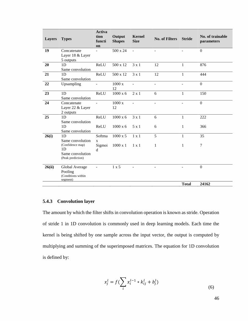
5.4.2 Modified U-net model
Intrinsically ECG contains mixtures of beats, conditions and sequence patterns. The
purpose of developing a U-net model is to extract localized information from the
heterogeneous ECG signal for beat wise analysis. In this project, the U-net is modified with
multiple classification heads, one head is used for R peak detection, while the others are

44
used for mapping out the conditions. Illustration of the modified U-net architecture is shown
in Figure 13 and Table 7 shows a sequential workflow of the newly proposed model.
Bulk of the proposed U-net is 1D convolution operations of kernel size 3 x 1. Unlike
conventional U-net model which uses valid convolution [62], we have applied same
convolution operation to obtain the output feature maps of the same size. Cropping is
therefore not required for the concatenation of feature maps. In total, this model has three
compression stages. During each compression, the features maps are halved and the number
of feature maps are doubled. In the expansive path, the high resolution features are being
copied from the contracting path directly and combined together with the up-sampled
features for subsequent convolutions, allowing the encoded context information to be
passed down to the subsequent layer effectively. At layer 25, 5 x 1 kernels are used for
convolving the R peak prediction branch, and 3 x 1 kernels are used in the confidence map
branch. Finally, 1 x 1 convolution is used in the last layer to reduce the number feature

45
maps to the corresponding training targets [93]. Since the model allows samples other than
those located at the R peaks to converge freely to any classes, a global average pooling layer
is added to the model during training time to prevent the confidence maps from converging
into any undesirable class that is not present in the segment.
Layers Types
Activa
tion
functi
on
Output
Shapes
Kernel
Size No. of Filters Stride
No. of trainable
parameters
0 Input - 1000 x 1 - - - 0
1 1D
Same convolution
ReLU 1000 x 6 3 x 1 6 1 24
2 1D
Same convolution
ReLU 1000 x 6 3 x 1 6 1 114
3 1D Max-pooling - 500 x 6 2 x 1 6 2 0
4 1D
Same convolution
ReLU 500 x 12 3 x 1 12 1 228
5 1D
Same convolution
ReLU 500 x 12 3 x 1 12 1 444
6 1D Max-pooling - 250 x 12 2 x 1 12 2 0
7 1D
Same convolution
ReLU 250 x 24 3 x 1 24 1 888
8 1D
Same convolution
ReLU 250 x 24 3 x 1 24 1 1752
9 1D Max-pooling - 125 x 24 2 x 1 24 2 0
10 1D
Same convolution
ReLU 125 x 48 3 x 1 48 1 3504
11 1D
Same convolution
ReLU 125 x 48 3 x 1 48 1 6960
12 Upsampling
- 250 x 48 - - - 0
13 1D
Same convolution
ReLU 250 x 24 2 x 1 24 1 2328
14 Concatenate
Layer 13 & Layer
8 outputs
- 250 x 48 - - - 0
15 1D
Same convolution
ReLU 250 x 24 3 x 1 24 1 3480
16 1D
Same convolution
ReLU 250 x 24 3 x 1 24 1 1752
17 Upsampling
- 500 x 24 - - - 0
18 1D
Same convolution
ReLU 500 x 12 2 x 1 12 1 588
46
Layers Types
Activa
tion
functi
on
Output
Shapes
Kernel
Size No. of Filters Stride
No. of trainable
parameters
19 Concatenate
Layer 18 & Layer
5 outputs
- 500 x 24 - - - 0
20 1D
Same convolution
ReLU 500 x 12 3 x 1 12 1 876
21 1D
Same convolution
ReLU 500 x 12 3 x 1 12 1 444
22 Upsampling
- 1000 x
12
- - - 0
23 1D
Same convolution
ReLU 1000 x 6 2 x 1 6 1 150
24 Concatenate
Layer 22 & Layer
2 outputs
- 1000 x
12
- - - 0
25 1D
Same convolution
1D
Same convolution
ReLU
ReLU
1000 x 6
1000 x 6
3 x 1
5 x 1
6
6
1
1
222
366
26(i) 1D
Same convolution (Confidence map)
1D
Same convolution (Peak prediction)
Softma
x
Sigmoi
d
1000 x 5
1000 x 1
1 x 1
1 x 1
5
1
1
1
35
7
26(ii) Global Average
Pooling (Conditions within segment)
- 1 x 5 -
- - 0
Total 24162
5.4.3 Convolution layer
The amount by which the filter shifts in convolution operation is known as stride. Operation
of stride 1 in 1D convolution is commonly used in deep learning models. Each time the
kernel is being shifted by one sample across the input vector, the output is computed by
multiplying and summing of the superimposed matrices. The equation for 1D convolution
is defined by:
𝑥𝑗𝑙 = 𝑓(∑𝑥𝑖
𝑙−1 ∗ 𝑘𝑖𝑗𝑙 + 𝑏𝑗
𝑙
𝑖
) (6)

47
where the * operator denotes convolution, xl-1 the output maps of the previous layer and xl
the output maps of the current layer. i is the corresponding kernel or feature map number
for the input while j is the corresponding kernel or feature map number for the output. b is
the bias added to the feature map and f is the activation function. During training, the
weights of the kernels are adjusted to pick up spatial patterns in the data.
5.4.4 Max pooling
In deep CNN structure, a convolution layer is usually followed by an immediate pooling
operation. Pooling is a type of quantization process, whereby the objective is to reduce the
size of the input representation by half or even lower. There are three commonly used
pooling operations, sum, average and max. Conventionally, max pooling has shown to
perform better in deep learning and is relatively easy to compute as compared to other
operations [74]. The output of the max-pooling layer is defined by the maximum value
within the non-overlapping predetermined filter size. In this case, the max pooling filter
size is set to 2 and the non-overlapping stride will eventually be 2.
5.4.5 Global pooling
Unlike conventional pooling operations, the filter size for global pooling operations is
defined the same as size of input. Thus the feature dimensionality of global pooled feature
map is vastly reduced by outputting only a single element.

48
In this project, global average pooling is used in the final layer of the U-net model for the
generation of class activation maps (CAM). Global average pooling was first described by
Lin et al. in [93]. The application was done by replacing the dense network structure with
global average pooling operations to generate a single class corresponding feature element
for classification. Instead of directly vectorizing the feature maps and feeding them into
fully connected layers for class prediction, each feature map is averaged and softmaxed.
This confirms the final layer of model to learn the correspondences between feature maps
and their respective categories. As a result, the visualization of class specific confidence
maps is easily achievable by plotting the feature maps from the final convolution layer.
Since global average pooling operation does not utilize any learnable parameters, the model
is forced to optimize through the learnable parameters from other layers. As a result, the
benefit of using such a layer is that it is less likely to overfit when compared to a fully
connected structure. Additionally, it averages the spatial information making the model to
be more invariant to spatial translations.
5.4.6 Long short term memory (LSTM)
The LSTM is a recurrent neural unit that has an input, memory state, and an output [86]. It
is useful for extracting temporal information from data. To calculate the memory state and
output of a LSTM unit, the below equations are used.
𝑖𝑡 = 𝜎(𝑊𝑖𝑥𝑡 + 𝑈𝑖ℎ𝑡−1 + 𝑏𝑖) (7)
𝑓𝑡 = 𝜎(𝑊𝑓𝑥𝑡 + 𝑈𝑓ℎ𝑡−1 + 𝑏𝑓) (8)

49
𝑜𝑡 = 𝜎(𝑊𝑜𝑥𝑡 + 𝑈𝑜ℎ𝑡−1 + 𝑏𝑜) (9)
𝑔𝑡 = 𝑡𝑎𝑛ℎ(𝑊𝑔𝑥𝑡 + 𝑈𝑔ℎ𝑡−1 + 𝑏𝑔) (10)
𝑐𝑡 = ⨀𝑐𝑡−1 + 𝑖𝑡⨀𝑔𝑡 (11)
ℎ𝑡 = 𝑜𝑡⨀𝑡𝑎𝑛ℎ(𝑐𝑡) (12)
where xt is the input, ht and ct are the outputs. The training parameters of LSTM are W, U
and b. σ represents the sigmoid function and tanh refers to the hyperbolic tangent function.
The ⊙ operator denotes Hadamard element-wise product while the input, forget and output
gates are defined as i, f and o respectively. At time, t = 0, ht and ct parameters are initialized
to 0.
5.4.7 Fully connected layer
Fully connected layer is commonly used in the final stage of the deep network for single
element prediction. The multi-tier dense structure is similar to the classical artificial neural
network and the computation for the fully connected layers is as follows.
𝑥𝑗𝑙 = 𝑓(∑𝑥𝑖
𝑙−1𝑤𝑖𝑗𝑙 + 𝑏𝑗
𝑙
𝑖
) (13)
where xl-1 denotes the outputs from the previous layer and xl the output for the current layer.
i is the corresponding neuron in the layer l -1 while j is corresponding neuron in the layer l.
b is the bias added to the multiplied inputs and f is the activation function used in layer l.

50
5.4.8 Activation function
The choice of activation functions is very important for deep network training. It can
directly affect the training dynamics of the model and the performance outcome. Currently,
the most successful and widely used activation function for deep network is the rectified
linear unit (ReLU). As compared to many other activation functions, deep networks with
many ReLU activated layers typically learns much faster. As such, it allows the deep
supervised network to be trained effectively without having the need to conduct any
unsupervised pre-training on the network itself [74]. The equation for the ReLU activation
function is defined as:
𝑓(𝑥) = max(0, 𝑥) (14)
Another common type of activation function used is the softmax function. It is applied in
the final layer of the fully connected structure to calculate the probability of distribution
across the multiple classes. The scores of each prediction is calculated by the softmax
function as follows:
𝑃𝑖 =
exp(𝑥𝑖)
∑ exp(𝑥𝑗)𝑁𝑜.𝑜𝑓𝐶𝑙𝑎𝑠𝑠𝑒𝑠𝑗=1
(15)
Pi is the probability score of a particular class while x is the input vector.

51
For binary problems, the sigmoid activation function is used. Sigmoid calculates the
probability of the output in the range of 0 to 1. Typically, the threshold value for binary
classifier is set to 0.5, if the output value of sigmoid function is over the threshold value it
is appointed as class 1, else the class is 0. The equation for sigmoid function is as follows.
𝜎(𝑥) =
1
1 + 𝑒−𝑥
(16)
5.4.9 Dropout regularization
Overfitting occurs when the variances between data are less. The model tend to picks up
unnecessary information such as noise artifacts during training, as a result the model fails
to generalize well.
In this project, two dropout regularization schemes (Scheme A and Scheme B) are employed
to prevent the CNN-LSTM network from overfitting. Dropout regularization is easy to
implement, during the training process part of the neurons in the network are randomly
removed. At each iteration, the neurons are removed and the loss will not be back
propagated, it is like creating a new model every time during training. This method allows
the model to learn from imperfection and thus prevents the model from adapting very well
to the training data [94].
5.4.10 Training and evaluation
In order to have a robust model, the networks are evaluated using ten-fold cross-validation
strategy. Stratified sampling method is used to divide the ECG dataset into 10 equal portions.

52
For the U-net dataset, the stratified sampling is carried out in accordance to the conditions
present in the segment such that each fold will have approximately the same number of
segments and conditions combination. Training of the network model uses 9 portions of the
ECG segments while testing uses the remaining portion. The procedure is repeated 10 times.
Each time the model is reinitialized and tested with a different data subset. In order to further
monitor the training progression of the models, 20% of the training set is isolated for
validation. Details for the ten-fold cross-validation is shown in Figure 14.
For each training fold, weights of the networks were initialized using the Xavier algorithm
[95]. All the models were trained end-to-end and the process was accelerated using
backpropagation algorithm with Adam optimizer [96]. The CNN-LSTM model is trained
with a batch size of 10 and the learning rate is 0.001. The modified U-net model is trained
with batch size of 20 and the learning rate is 0.0005. For batch training, the steps which
involved in the backpropagation are very much similar to equations (1-4). Gradients
calculated from multiple samples are cumulated and then averaged for batch updating. In

53
order to combat the class imbalance problem, a weighted class variable α is introduced to
the loss calculation. The calculation of weighted variable for each class is accomplished by
the scikit-learn library [97]. The formula for yielding the class weight is given by
𝛼𝑖 =
𝑡𝑜𝑡𝑎𝑙𝑛𝑜. 𝑜𝑓𝑠𝑎𝑚𝑝𝑙𝑒𝑠
(𝑡𝑜𝑡𝑎𝑙𝑛𝑜. 𝑜𝑓𝑐𝑙𝑎𝑠𝑠𝑒𝑠 ∗ 𝑛𝑜. 𝑜𝑓𝑠𝑎𝑚𝑝𝑙𝑒𝑠𝑓𝑜𝑟𝑚𝑐𝑙𝑎𝑠𝑠𝑖)
(17)
αi is the weighted variable for class i and the ith class is represented as classi .
There are two types of losses (cross entropy and binary cross entropy) used in this project.
The prediction for the ECG conditions is done using softmax classification and the loss is
calculated using the cross entropy formula given below
𝐶𝑟𝑜𝑠𝑠𝐸𝑛𝑡𝑟𝑜𝑝𝑦𝐿𝑜𝑠𝑠 = − ∑ 𝛼𝑖𝑇𝑖𝑙𝑜𝑔𝑃𝑖
𝑁𝑜.𝑜𝑓𝐶𝑙𝑎𝑠𝑠𝑒𝑠
𝑖=1
(18)
α is the weighted class variable, T is the one hot encoded class label and P is the class
probabilities that is calculated from equation (15).
R peak prediction is in binary form. Therefore binary cross entropy loss is used:
𝐵𝑖𝑛𝑎𝑟𝑦𝐶𝑟𝑜𝑠𝑠𝐸𝑛𝑡𝑟𝑜𝑝𝑦𝐿𝑜𝑠𝑠 = −𝛼1𝑇𝑙𝑜𝑔𝑃 + 𝛼0(1 − 𝑇)log(1 − 𝑃) (19)
α is the weighted class variable, T is the binary label and P is the binary output probability
that is calculated the sigmoid function.

54
Performances for each fold is measured based on the accuracy (ACC), sensitivity (SEN),
specificity (SPEC) and positive predictive value (PPV). The computation of these
performance measures are given by equations (20-23).
𝐴𝐶𝐶(%) =
𝑇𝑃 + 𝑇𝑁
𝑇𝑃 + 𝑇𝑁 + 𝐹𝑃 + 𝐹𝑁∗ 100
(20)
𝑆𝐸𝑁(%) =
𝑇𝑃
𝑇𝑃 + 𝐹𝑁∗ 100
(21)
𝑆𝑃𝐸𝐶(%) =
𝑇𝑁
𝑇𝑁 + 𝐹𝑃∗ 100
(22)
𝑃𝑃𝑉(%) =
𝑇𝑃
𝑇𝑃 + 𝐹𝑃∗ 100
(23)
where TN (true negative) refers to true negative as the number of healthy data correctly
classified as healthy. TP (true positive) indicates the number of correctly classified as
arrhythmias. FN (false negative) suggests the number of healthy data misclassified as
arrhythmias. FP (false positive) signifies the number of arrhythmias data misclassified as
healthy. After each fold, these performance measures and computed. Then the average of
ten-folds are computed and expressed as the overall performance of the proposed system.

55
6 CHAPTER SIX – RESULTS & DISCUSSION
6.1 RESULTS
In this project, the deep learning networks are developed in python using Keras [98] for
easy prototyping and Tensorflow as the backend deep learning library [99]. The
specification of the workstation used for training the models consists of two Intel Xeon 2.40
GHz (E5620) processors and a 24GB RAM.
6.1.1 CNN-LSTM
Each training epoch took approximately 138.12 seconds for the CNN-LSTM model to
finish. During vanilla testing, it is found out that the CNN-LSTM model tend to overfit the
training data. In order to improve the generalization ability, two dropout schemes are
proposed for testing. For each scheme different parts of the network are being dropped.
Scheme A has 20% dropout applied to the LSTM recurrent and input connections while
Scheme B has 20% dropout applied to the LSTM recurrent connections and the two densely
connected layers. The learning curves for the dropout schemes are shown in Figure 15.

56
Signs of overfitting can be observed from learning curves of the vanilla CNN-LSTM. It is
clear that after 25 epochs, the validation curves plateau, while the training curve rises
continuously. Accuracy curves for dropout networks on the other hand are relatively stable.
In both plots the accuracy curves are seen rising gradually and eventually converged at 150
epochs.
Table 8 shows the average of all the ten-fold cross-validation results obtained from the
proposed CNN-LSTM models. It is observed that the over fitted vanilla model has yielded
the highest performance among all across while Scheme A has yielded the lowest

57
performance among all. Also, it should be noted that the computed standard deviation for
all the performance results are found to be the least for Scheme B
Figure 16 and Figure 17 are the confusion matrixes of Scheme A and B respectively.
Comparing the confusion matrixes of the two models, it can be determined that Scheme A
is marginally better at predicting the PVC class, while Scheme B is a better predictor of
normal, APB, LBBB and RBBB classes. Looking at the diagonal elements of the confusion
matrixes, the result of both the models are very much close to each other. The slightly poor
result for Scheme A could be due to the application of dropout at the input and output of
the LSTM which leads to higher error rate.
Both the CNN-LSTM models have failed in classifying the normal and APB segments
correctly, consistently mixing up the cardiac conditions. It is observed that 1.8% of the APB
segments are misclassified as other conditons in Scheme A, while 1.3 % of the APB
segments are misclassified as other conditons in Scheme B. This could be due to the subtle
amplitude differences between ectopic and normal P wave. Moreover, the presence of noise
artifacts in the signals makes it even harder for the models to detect.

58
6.1.2 Modified U-net
The U-net model is trained for 200 epochs, each training epoch of the modified U-net model
took approximately 120.13 seconds to execute. The accuracy curves for beats classification
and R peak detection averaged across all 10 folds are depicted in Figure 18. Accuracy for
classifying the beats condition is evaluated based on the annotations provided at the R peaks.

59
It can be seen from Figure 18 that, the proposed U-net model is able to generalize well from
the training data without any additional network regularization. No sign of overfitting is
observed as both learning curves from the plots are seen relatively close to each other. Few
factors may have contributed to the good generalization ability of the modified U-net. First,
the data used for training and testing the U-net is much more diversified and complex due
to the multitude of conditions present in each ECG segments. Second, when compared to
the CNN-LSTM model, the proposed U-net model has kernels that are smaller in size. The
use of smaller kernels also mean that the number of learnable parameters used are lesser
hence, the chances of the model suffering from overfitting is reduced. Lastly, it may be due
to the inclusion of global average pooling. Global average pooling itself is a structural
regularizer and does not utilize any learnable parameter. The model is forced to learn from
the averaged information and thus minimizes the chances of overfitting.
Generally, the training and validation accuracies obtained from the two classification heads
are fairly stable. The accuracy curves for ECG beats classification can be seen plateauing
after 50 epochs whereby the model is unable to progress any further from the traning. The

60
accuracy curves for R peak identification declined slightly after training for 75 epochs. This
could be due to the gradient descent of the learning model escape from the global minimum
and got stuck in a valley that is sub-optimal. The overall cross validation performances for
the modified U-net is summarized in Table 9.
On average the proposed U-net was able to identify the beats condition correctly with an
accuracy of 97.32% and 99.3% in predicting the R peaks. The confusion matrix for beats
classification and R peak prediction are presented in Figure 19 and Figure 20 respectively.
It can be observed in Figure 19 that the proposed model is able to identify most of the ECG
beats conditions (normal, LBBB, RBBB and PVC) correctly with an accuracy of above 90%
except for APB class. However, almost half of the APB beats are misclassified either either
as normal or RBBB. The poor classification result of the APB class maybe due to the subtle
changes between the P waves of an ectopic and normal beats. Also, when the P wave of
ectopic superimposed on the preceding T wave, the network fails to differentiate it as
preceding T wave. The network therefore treats the superimposed wave as P wave causing
the network to misclassify. In addition, due to the lack of diversity, the model may have
failed in recognizing the underlying features of the APB class since APB has the lowest
number of beats among all the classes.

61
The confusion matrix for R peaks prediction depicted in Figure 20 shows that, the algorithm
is able to identify both the non-R peak and R peak samples with an accuracy of 99%. The
low sensitivity of 29.55% for the R peak prediction is caused due to the misclassification
of surrounding samples of the R peaks. It can be observed in Figure 21 (b) that, not only
the maxima of normal beat but also the surrounding samples are predicted as the R peak.
Additionally, when the beat has a wide QRS complex with a small positive R wave followed
by large negative S wave, the algorithm classifies both extrema and sometimes the samples
in-between as the R peaks. This phenomenon is frequently observed in the prediction of R
peak in PVC beats. The examples of such cases are shown in Figure 21 (a) and (b).
In Figure 21, four test ECG segments and their activation maps are presented. Each of these
activation maps correspond to a condition in which the most discriminative regions within
the segments are highlighted in red. Through the visualization of the activation maps, it is

62
clear that the U-net has the ability to identify most of the classes except APB class. Several
subsequences of normal, PVC, LBBB and RBBB beats are highlighted in the appropriate
regions. It is evident that the model has demonstrated good localization capability with the
correct attentions taken by the network during classification.

63
6.2 DISCUSSION
During our preliminary study, the CNN-LSTM model is proposed to classify varying
lengths ECG signals. The CNN is typically useful in picking up the spatial features while
LSTM the able to understand the temporal dynamics within the data. Hence, we have
decided to merge these two modalities for better diagnostic accuracy.
Like most machine learning algorithms, the hybrid model quickly over fits the data during
training phase. Over fitted models usually underperform when tested against a new dataset
[100]. In total, two dropout regularization schemes are introduced and tested. It is found
that, the dropping of 20% recurrent connections in LSTM and densely connected layers has
provided better generalization ability. On top of more stable performance, the low standard
deviation values in Table 8 indicates that the calculated performance measures across the
folds are relatively close to each other.
The CNN-LSTM has achieved good classification results of 98.10% accuracy, by assuming
that each ECG segments consists of only one type of arrhythmia. In the reality this is not
always true, as the ECG signal can contain mixtures of multiple beat types. In order to deal
with this problem, the U-net model is explored in the latter part of this project.
The U-net model was initially developed for image segmentation. In order for the model to
classify the ECG beats using only the annotations provided at the R peaks. We have
modified the model by having multiple classification heads. One head is used to detect the
R peaks, while the other is used to identify the conditions in the time series. A global

64
average pooling layer is also added to the final layer of the U-net to obtain the class
activation maps for each condition. The proposed U-net model has shown good
generalization ability with no signs of overfitting during training. Additionally, the results
obtained from the modified U-net are found to be promising. The accuracy for classifying
the conditions of individual beats according to the annotations provided at the R peak is
97.32% while the accuracy for detecting the R peak is 99.3%. Visualization of class
activation maps in Figure 21 also shows that the model is capable of differentiating the
segments into subsequences and associating them with correct conditions.
Ultimately, the benefits of implementing a deep learning network is to minimize the number
of preprocessing techniques required, allowing the system to be trained end to end. The
newly developed U-net model is much superior as compared to the CNN-LSTM model
since it does not make any assumptions to the input segments. Theoretically, all the
operations used in the U-net have the ability to handle variable length data unlike the fully
connected layers used in CNN-LSTM model which can only deal with input of a fixed
length size.
The advantages of the newly proposed modified U-net model are as follows:
1. Proposed system is fully automated.
2. Observer bias is eliminated.
3. End-to-end solution, requires minimal processing.
4. Standalone classification heads for R peaks detection and classification of ECG
conditions.

65
5. Localized predictions.
6. Robustness of system is assessed by cross validations testing.
7. Class activation maps provide information about the localization and instances for
beat predictions.
The drawbacks of the newly proposed algorithm however are:
1. Subtle changes and overlapping of waves leads to misclassification of APB class.
2. Training phase is computationally intensive and slow.
3. Very few APB class ECG data are available as compared to other classes.
4. The model is trained and tested using an imbalance dataset.
5. Predictions for R peak is not robust.

66
7 CHAPTER SEVEN – CONCLUSION & FUTURE WORK
7.1 CONCLUSION
Early diagnosis of cardiac abnormalities is important as prolonged arrhythmias increase the
risk of other cardiac diseases and mortality. Effective screening system can aid clinicians
in diagnosing the conditions early and provide the patients with proper care and timely
intervention. Current standard for arrhythmias screening involves visual examination and
manual interpretation of ECG records by clinicians. This process is labor intensive,
mundane and vulnerable to inter-observer variability. Moreover, changes within ECG
signals are small and often not noticeableby for the average person. Hence, computer
automated system may assist in the early objective screening of arrhythmic ECGs.
In this research project, two novel deep learning models are developed to screen the ECGs
records automatically. The first system detects the heart conditions by using state-of-art
techniques (CNN and LSTM) found in the literature studies. The hybrid system has attained
classification accuracy of as high as 98.10% with variable length of ECGs. The second
system is a modified U-net model that uses multiple classification heads to access the beats
conditions individually.
To the best of author’s knowledge this is the first research to experiment with deep learning
autoencoder for ECG beats wise classification. The newly proposed U-net has attained
highest classification accuracy of 97.32% in diagnosing the cardiac conditions and 99.3%
for R peak detection without noise elimination. It is also demonstrated that the automated

67
system is capable of self-learning and generating useful class activations maps
differentiating the conditions in relation to each ECG cardiac cycle.

68
7.2 FUTURE WORK
The future work includes acquisition of more ECG record and redesigning the U-net model.
The current U-net model is not accurate in predicting the R peaks whereby multiple samples
around the R peak are misclassified. A thresholding layer can thus be added after the R peak
classification head to limit the number of R peak samples detected within a predefined
striding window, this can help to improve the sensitivity for R peaks detection. The same
can also be applied to the activation maps to help improve in the resolution.
U-net does not consist of any fully connected layers, thus the inputs can be of any length
size. Unlike fully connected layers which require a fixed input and output size, the output
of the U-net is completely dependent on the local area of input. In future it is feasible for
the network to be tested on data of any length without the need of zero padding.
Also, instead of using a weighted parameter to balance the loss, data augmentation can be
implemented to counter the class imbalance problem [101]. ECG data augmentation is a
complex problem, one cannot simply apply dynamic warping to generate a synthetic data.
Stretching or compressing an ECG data without understanding the underlying context may
induce distortion on the data and may result in wrong annotated data. Generative adversarial
network (GAN) can be a good solution as it is able to learn the underlying discriminators
of the various cardiac conditions and generate realistic ECG database on them.

69
Training of deep learning network requires massive amounts of computational power. In
this project we have trained the networks solely on the central processing unit (CPU) of the
workstation. Graphics processing units (GPUs) can be utilized in the future to accelerate
the training process of the U-net model so that more data can be tested. Finally, other cardiac
diseases like ischemic heart disease and congestive heart failure can also be explored.

70
REFERENCES
1. Zimetbaum, P. and A. Goldman, Ambulatory Arrhythmia Monitoring. Choosing the Right
Device, 2010. 122(16): p. 1629-1636. 2. Nations, U., World population ageing 2017 Highlights. New York: Department of Economic
and Social Affairs, 2017. 3. Chow, G.V., J.E. Marine, and J.L. Fleg, Epidemiology of Arrhythmias and Conduction
Disorders in Older Adults. Clinics in geriatric medicine, 2012. 28(4): p. 539-553. 4. Mak, K., The Normal Physiology of Aging, in Colorectal Cancer in the Elderly, K.-Y. Tan,
Editor. 2013, Springer Berlin Heidelberg: Berlin, Heidelberg. p. 1-8. 5. Anversa, P., et al., Myocyte cell loss and myocyte cellular hyperplasia in the hypertrophied
aging rat heart. Circulation Research, 1990. 67(4): p. 871-885. 6. Schneider, J.F., et al., Newly acquired left bundle-branch block: The framingham study.
Annals of Internal Medicine, 1979. 90(3): p. 303-310. 7. Fahy, G.J., et al., Natural history of isolated bundle branch block. The American Journal of
Cardiology, 1996. 77(14): p. 1185-1190. 8. Thrainsdottir, I.S., et al., The epidemiology of right bundle branch block and its association
with cardiovascular morbidity — The Reykjavik Study. European Heart Journal, 1993. 14(12): p. 1590-1596.
9. Binici, Z., et al., Excessive Supraventricular Ectopic Activity and Increased Risk of Atrial Fibrillation and Stroke. Circulation, 2010. 121(17): p. 1904.
10. Engström, G., et al., Cardiac Arrhythmias and Stroke. Stroke, 2000. 31(12): p. 2925. 11. Fleg, J.L. and H.L. Kennedy, Cardiac Arrhythmias in a Healthy Elderly Population. CHEST.
81(3): p. 302-307.
12. Francia, P., et al., Left bundle‐branch block—pathophysiology, prognosis, and clinical management. Clinical Cardiology, 2007. 30(3): p. 110-115.
13. Schneider, J.F., et al., Newly acquired right bundle-branch block: The framingham study. Annals of Internal Medicine, 1980. 92(1): p. 37-44.
14. Conen, D., et al., Premature Atrial Contractions in the General Population Frequency and Risk Factors. Circulation, 2012. 126(19): p. 2302.
15. Perez, M.V., et al., Electrocardiographic predictors of atrial fibrillation. American Heart Journal. 158(4): p. 622-628.
16. Wallmann, D., et al., Frequent Atrial Premature Beats Predict Paroxysmal Atrial Fibrillation in Stroke Patients. Stroke, 2007. 38(8): p. 2292.
17. Healey, J.S., et al., Subclinical Atrial Fibrillation and the Risk of Stroke. New England Journal of Medicine, 2012. 366(2): p. 120-129.
18. Inoue, K., et al., Trigger-Based Mechanism of the Persistence of Atrial Fibrillation and Its Impact on the Efficacy of Catheter Ablation. Circulation: Arrhythmia and Electrophysiology, 2012. 5(2): p. 295.
19. Manolio, T.A., et al., Cardiac arrhythmias on 24-h ambulatory electrocardiography in older women and men: The cardiovascular health study. Journal of the American College of Cardiology, 1994. 23(4): p. 916-925.
20. Kantelip, J.-P., E. Sage, and P. Duchene-Marullaz, Findings on ambulatory electrocardiographic monitoring in subjects older than 80 years. American Journal of Cardiology. 57(6): p. 398-401.

71
21. Messineo, F.C., Ventricular ectopic activity: Prevalence and risk. American Journal of Cardiology. 64(20): p. J53-J56.
22. Kostis, J.B., et al., Premature ventricular complexes in the absence of identifiable heart disease. Circulation, 1981. 63(6): p. 1351.
23. Fleg, J.L. and E.G. Lakatta, Prevalence and prognosis of exercise-induced nonsustained ventricular tachycardia in apparently healthy volunteers. American Journal of Cardiology. 54(7): p. 762-764.
24. Aronow, W.S., et al., Usefulness of echocardiographic abnormal left ventricular ejection fraction, paroxysmal ventricular tachycardia and complex ventricular arrhythmias in predicting new coronary events in patients over 62 years of age. American Journal of Cardiology. 61(15): p. 1349-1351.
25. Bikkina, M., M.G. Larson, and D. Levy, Prognostic implications of asymptomatic ventricular arrhythmias: The framingham heart study. Annals of Internal Medicine, 1992. 117(12): p. 990-996.
26. Goldberger, A.L., et al., PhysioBank, PhysioToolkit, and PhysioNet. Components of a New Research Resource for Complex Physiologic Signals, 2000. 101(23): p. e215-e220.
27. Yeh, Y.-C., W.-J. Wang, and C.W. Chiou, Cardiac arrhythmia diagnosis method using linear discriminant analysis on ECG signals. Measurement, 2009. 42(5): p. 778-789.
28. Li, T. and M. Zhou, ECG Classification Using Wavelet Packet Entropy and Random Forests. Entropy, 2016. 18(8).
29. Sahoo, S., et al., Multiresolution wavelet transform based feature extraction and ECG classification to detect cardiac abnormalities. Measurement, 2017. 108: p. 55-66.
30. Karimifard, S. and A. Ahmadian, A robust method for diagnosis of morphological arrhythmias based on Hermitian model of higher-order statistics. BioMedical Engineering OnLine, 2011. 10: p. 22-22.
31. Osowski, S., L.T. Hoai, and T. Markiewicz, Support vector machine-based expert system for reliable heartbeat recognition. IEEE Transactions on Biomedical Engineering, 2004. 51(4): p. 582-589.
32. Elhaj, F.A., et al., Arrhythmia recognition and classification using combined linear and nonlinear features of ECG signals. Computer Methods and Programs in Biomedicine, 2016. 127: p. 52-63.
33. Li, H., et al., Arrhythmia Classification Based on Multi-Domain Feature Extraction for an ECG Recognition System. Sensors (Basel, Switzerland), 2016. 16(10): p. 1744.
34. Martis, R.J., U.R. Acharya, and L.C. Min, ECG beat classification using PCA, LDA, ICA and Discrete Wavelet Transform. Biomedical Signal Processing and Control, 2013. 8(5): p. 437-448.
35. Martis, R.J., et al., Cardiac decision making using higher order spectra. Biomedical Signal Processing and Control, 2013. 8(2): p. 193-203.
36. Martis, R.J., et al. Application of higher order cumulants to ECG signals for the cardiac health diagnosis. in 2011 Annual International Conference of the IEEE Engineering in Medicine and Biology Society. 2011.
37. Martis, R.J., et al., Application of principal component analysis to ECG signals for automated diagnosis of cardiac health. Expert Systems with Applications, 2012. 39(14): p. 11792-11800.
38. Yu, S.-N. and K.-T. Chou, Integration of independent component analysis and neural networks for ECG beat classification. Expert Systems with Applications, 2008. 34(4): p. 2841-2846.

72
39. Akkus, Z., et al., Deep Learning for Brain MRI Segmentation: State of the Art and Future Directions. Journal of Digital Imaging, 2017. 30(4): p. 449-459.
40. Pham, T., et al., Predicting healthcare trajectories from medical records: A deep learning approach. Journal of Biomedical Informatics, 2017. 69: p. 218-229.
41. Acharya, U.R., et al., Automated detection of arrhythmias using different intervals of tachycardia ECG segments with convolutional neural network. Information Sciences, 2017. 405: p. 81-90.
42. Acharya, U.R., et al., A deep convolutional neural network model to classify heartbeats. Computers in Biology and Medicine, 2017. 89: p. 389-396.
43. Zubair, M., J. Kim, and C. Yoon. An Automated ECG Beat Classification System Using Convolutional Neural Networks. in 2016 6th International Conference on IT Convergence and Security (ICITCS). 2016.
44. Kiranyaz, S., T. Ince, and M. Gabbouj, Real-Time Patient-Specific ECG Classification by 1-D Convolutional Neural Networks. IEEE Transactions on Biomedical Engineering, 2016. 63(3): p. 664-675.
45. Yildirim, Ö., A novel wavelet sequence based on deep bidirectional LSTM network model for ECG signal classification. Computers in Biology and Medicine, 2018. 96: p. 189-202.
46. Qian, Y., et al., Very Deep Convolutional Neural Networks for Noise Robust Speech Recognition. IEEE/ACM Transactions on Audio, Speech, and Language Processing, 2016. 24(12): p. 2263-2276.
47. Acharya, U.R., et al., Application of deep convolutional neural network for automated detection of myocardial infarction using ECG signals. Information Sciences, 2017. 415-416: p. 190-198.
48. Wu, Y., et al., Google's Neural Machine Translation System: Bridging the Gap between Human and Machine Translation. 2016.
49. Kim, M., et al., Speaker-Independent Silent Speech Recognition From Flesh-Point Articulatory Movements Using an LSTM Neural Network. IEEE/ACM Transactions on Audio, Speech, and Language Processing, 2017. 25(12): p. 2323-2336.
50. Song, E., F.K. Soong, and H.G. Kang, Effective Spectral and Excitation Modeling Techniques for LSTM-RNN-Based Speech Synthesis Systems. IEEE/ACM Transactions on Audio, Speech, and Language Processing, 2017. 25(11): p. 2152-2161.
51. Sundermeyer, M., H. Ney, and R. Schlüter, From Feedforward to Recurrent LSTM Neural Networks for Language Modeling. IEEE/ACM Transactions on Audio, Speech, and Language Processing, 2015. 23(3): p. 517-529.
52. Greff, K., et al., LSTM: A Search Space Odyssey. IEEE Transactions on Neural Networks and Learning Systems, 2017. 28(10): p. 2222-2232.
53. Yang, W., et al. Improved deep convolutional neural network for online handwritten Chinese character recognition using domain-specific knowledge. in 2015 13th International Conference on Document Analysis and Recognition (ICDAR). 2015.
54. Zhang, X.Y., et al., End-to-End Online Writer Identification With Recurrent Neural Network. IEEE Transactions on Human-Machine Systems, 2017. 47(2): p. 285-292.
55. Tan, J.H., et al., Application of stacked convolutional and long short-term memory network for accurate identification of CAD ECG signals. Computers in Biology and Medicine, 2018. 94: p. 19-26.
56. Oh, S.L., et al., Automated diagnosis of arrhythmia using combination of CNN and LSTM techniques with variable length heart beats. Computers in biology and medicine, 2018.
57. Hinton, G.E. and R.R. Salakhutdinov, Reducing the dimensionality of data with neural networks. science, 2006. 313(5786): p. 504-507.

73
58. Yildirim, O., R.S. Tan, and U.R. Acharya, An efficient compression of ECG signals using deep convolutional autoencoders. Cognitive Systems Research, 2018. 52: p. 198-211.
59. Testa, D.D. and M. Rossi, Lightweight Lossy Compression of Biometric Patterns via Denoising Autoencoders. IEEE Signal Processing Letters, 2015. 22(12): p. 2304-2308.
60. Xiong, P., et al., A stacked contractive denoising auto-encoder for ECG signal denoising. Physiological measurement, 2016. 37(12): p. 2214.
61. Guo, Y., et al., A review of semantic segmentation using deep neural networks. International Journal of Multimedia Information Retrieval, 2017.
62. Ronneberger, O., P. Fischer, and T. Brox. U-net: Convolutional networks for biomedical image segmentation. in International Conference on Medical image computing and computer-assisted intervention. 2015. Springer.
63. Lei, Y., et al., A skin segmentation algorithm based on stacked autoencoders. IEEE Transactions on Multimedia, 2017. 19(4): p. 740-749.
64. Xing, F., et al., Deep Learning in Microscopy Image Analysis: A Survey. IEEE Transactions on Neural Networks and Learning Systems, 2017.
65. Pappano, A.J. and W. Gil Wier, 1 - Overview of the Circulation and Blood, in Cardiovascular Physiology (Tenth Edition). 2013, Content Repository Only!: Philadelphia. p. 1-9.
66. Pappano, A.J. and W. Gil Wier, 4 - The Cardiac Pump, in Cardiovascular Physiology (Tenth Edition). 2013, Content Repository Only!: Philadelphia. p. 55-90.
67. Pappano, A.J. and W. Gil Wier, 3 - Automaticity: Natural Excitation of the Heart, in Cardiovascular Physiology (Tenth Edition). 2013, Content Repository Only!: Philadelphia. p. 31-53.
68. Boullin, J. and J.M. Morgan, The development of cardiac rhythm. Heart, 2005. 91(7): p. 874-875.
69. Reynolds, P., Chapter 43 - Cardiac arrhythmias and conduction disturbances A2 - Kauffman, Timothy L, in Geriatric Rehabilitation Manual (Second Edition), J.O. Barr and M. Moran, Editors. 2007, Churchill Livingstone: Edinburgh. p. 265-274.
70. Alemzadeh-Ansari, M.J., Chapter 3 - Electrocardiography A2 - Maleki, Majid, in Practical Cardiology, A. Alizadehasl and M. Haghjoo, Editors. 2018, Elsevier. p. 17-60.
71. Yadav, N., A. Yadav, and M. Kumar, An introduction to neural network methods for differential equations. 2015: Springer.
72. Barrow, H., Chapter 5 - Connectionism and Neural Networks A2 - Boden, Margaret A, in Artificial Intelligence. 1996, Academic Press: San Diego. p. 135-155.
73. Haykin, S., Neural Networks: A Comprehensive Foundation (3rd Edition). 2007: Prentice-Hall, Inc.
74. LeCun, Y., Y. Bengio, and G. Hinton, Deep learning. Nature, 2015. 521: p. 436. 75. Kahali, S., S.K. Adhikari, and J.K. Sing, Convolution of 3D Gaussian surfaces for volumetric
intensity inhomogeneity estimation and correction in 3D brain MR image data. IET Computer Vision, 2018. 12(3): p. 288-297.
76. Li, Q., Q. Peng, and C. Yan, Multiple VLAD Encoding of CNNs for Image Classification. Computing in Science & Engineering, 2018. 20(2): p. 52-63.
77. Zhang, F., et al., Image denoising method based on a deep convolution neural network. IET Image Processing, 2018. 12(4): p. 485-493.
78. Zhang, J. and Y. Wu, A New Method for Automatic Sleep Stage Classification. IEEE Transactions on Biomedical Circuits and Systems, 2017. 11(5): p. 1097-1110.
79. Zhang, Q., D. Zhou, and X. Zeng, HeartID: A Multiresolution Convolutional Neural Network for ECG-Based Biometric Human Identification in Smart Health Applications. IEEE Access, 2017. 5: p. 11805-11816.

74
80. Hubel, D.H. and T.N. Wiesel, Receptive fields and functional architecture of monkey striate cortex. The Journal of Physiology, 1968. 195(1): p. 215-243.
81. Fukushima, K., Neocognitron: A self-organizing neural network model for a mechanism of pattern recognition unaffected by shift in position. Vol. 36. 1980. 193-202.
82. Wiatowski, T. and H. Bölcskei, A Mathematical Theory of Deep Convolutional Neural Networks for Feature Extraction. Vol. PP. 2015.
83. Mallat, S., Group Invariant Scattering. Vol. 65. 2012. 84. Lipton, Z.C., J. Berkowitz, and C. Elkan, A critical review of recurrent neural networks for
sequence learning. arXiv preprint arXiv:1506.00019, 2015. 85. Bengio, Y., P. Simard, and P. Frasconi, Learning long-term dependencies with gradient
descent is difficult. IEEE Transactions on Neural Networks, 1994. 5(2): p. 157-166. 86. Hochreiter, S., #252, and r. Schmidhuber, Long Short-Term Memory. Neural Comput., 1997.
9(8): p. 1735-1780. 87. Ciresan, D., et al. Deep neural networks segment neuronal membranes in electron
microscopy images. in Advances in neural information processing systems. 2012. 88. Wojna, Z., et al., The devil is in the decoder. arXiv preprint arXiv:1707.05847, 2017. 89. Hermes, R.E., D.B. Geselowitz, and G.C. Oliver, Development, distribution, and use of the
American Heart Association database for ventricular arrhythmia detector evaluation. 90. Moody, G.B. and R.G. Mark, The impact of the MIT-BIH Arrhythmia Database. IEEE
Engineering in Medicine and Biology Magazine, 2001. 20(3): p. 45-50. 91. Conover, M.B., Understanding Electrocardiography. 2002: Mosby. 92. LeCun, Y., et al., Efficient BackProp, in Neural Networks: Tricks of the Trade, this book is an
outgrowth of a 1996 NIPS workshop. 1998, Springer-Verlag. p. 9-50. 93. Lin, M., Q. Chen, and S. Yan, Network in network. arXiv preprint arXiv:1312.4400, 2013. 94. Srivastava, N., et al., Dropout: A Simple Way to Prevent Neural Networks from Overfitting.
Vol. 15. 2014. 1929-1958. 95. Bengio, Y. and X. Glorot, Understanding the difficulty of training deep feed forward neural
networks. 2010. 249-256. 96. Kingma, D.P. and J. Ba, Adam: A method for stochastic optimization. arXiv preprint
arXiv:1412.6980, 2014. 97. Pedregosa, F., et al., Scikit-learn: Machine learning in Python. Journal of machine learning
research, 2011. 12(Oct): p. 2825-2830. 98. Chollet, F., Keras. 2015. 99. Abadi, M., et al. TensorFlow: A System for Large-Scale Machine Learning. in OSDI. 2016. 100. Hawkins, D.M., The Problem of Overfitting. Journal of Chemical Information and Computer
Sciences, 2004. 44(1): p. 1-12. 101. C. Wong, S., et al., Understanding Data Augmentation for Classification: When to Warp?
2016. 1-6.
75
APPENDIX A: PUBLISHED PAPERS
1. Oh, S.L., et al., Automated diagnosis of arrhythmia using combination of CNN and
LSTM techniques with variable length heart beats. Computers in biology and
medicine, 2018. https://doi.org/10.1016/j.compbiomed.2018.06.002
2. Oh, S.L., et al., Automated beat-wise arrhythmia diagnosis using modified U-net on
extended electrocardiographic recordings with heterogeneous arrhythmia types.
Submitted to Computers in biology and medicine.