AD-A286 161

ARMY RESEARcH LABORATORY •

Application of Chimera Techniqueto Projectiles in Relative Motion

Jubaraj SahuCharles J. Nietubicz

ARL-TR-590 October 1994

C...:; .* . •2,• 6v

AP•ROVED PIW C RE•.EAW. DISTWUTION 0 UNMUiTle

".*\Ž" 94-35260

~!wj~i1~t9 4I,*

NOTICES

Destroy this report when It is no longer needed. DO NOT return it to the originator.

Additional copies of this teport may be obtalned from the Nsmtal Technical InformationService, U.S. Depament of Commerce. 5219 Port Royal Road, Springfield. VA 22161.

The findings of this report are not to be ,onstrued as an official Department of the Armyposition, unless so designated by other authorized doc.ments.

The use of trade names or manufacturers' names in his report does not constituteindorsement of any commercial product.

REPORT DOCUMENTATION PAGE OU NO.m Approve

~~' - - ffmm- -a ma to qI 1_1 m~sU.I =1 Imkqw. ifts eai 11.~I We .i.i -4 *Iniy daft news".i

AGENCY tin ONL.Y (Lafw b&WMJ 2. E £R 2.; AN -'ESCOVERED

ROctober 1994 Final. February 1993 - May 19944 TI[ NDWAYLES. FUNDN NUMGERS

Application ot Chimera Technique to Proicectilcs in Relative Motion PR: IL16110O2AH43* WO: 61102A-OO-00I-AJ1

* Jutbara Sahu and Charles J Nictubiicr

7 0M1104 ORGANIZATION NAME4S) X0D ADOREWES) AFFIWORIN 0111ANIAT1O

ITS Army Rescanch Lhtaboaory 11EPO1 T NUMBER

A1TN AMSRLWT*-PBAberdeen Proving Ground. MD) 21005-5066

1 SV OLSMIG0NIT 611ORINO AGENCY NAMES(SI) AND AOPEREES) 110.111ONS3ROK640eeITORINGAGENCY REPIOIIT NUMBER

ITS Army Research LaboratoryATTN AMSRI.-OP-AP-1, ARL-TR-590Aherdeen Proving (;round, MD) 2 1(X5 5066

11. SUPPLEMENTARY NOTES

12s. DISTRIBUTIOWAVAILABWUTY STATEMENT 12b. DISTRIBUTION CODE

Approved for public release; distribution i unh iiited.

13. ABSTRACT (Maximum 200 words)

This report describes the application of the versatile Chimera numerical technique to a time-diependent, muftibodyprojectile configuration. A computational study was performed to determine the aerodynamics of small cylindricalsegments being ejected into (he wake of a flared projectile, The complexity and uniqueness of this problem results fromthe segments being in relative motion to each other, embedded in a nonuniform wake flow, and requiring a time-dependent solution. Flow field computations for this multibody problem have been performed for supersonic conditions.The predicted flow field over the segments was found to undergo significant changes as the segments separated from theparent projectile. Comparison of the unsteady Chimera results with the quasi-static approach shows the difference in draghistory to be significant which indicates the need for time-dependent solution techniques. A subsequent experimcntalprogram was Londucted in the Army Research Laboratory's (ARL) Transoriic Range and the computed segment positionsand velocities were found to be in good agreement with the experimental data.

14. SUBJECT TERMS 15. NUMBER OF PAGES

Aerodynamics; multiple bodies; unsteady flow; Chimera; wake; drag 3016. PRICE CODE

17. SECURITY CLASSIFICATION is. SECURITY CLASSIFICATION 19. SECURITY CLASSIFICATION 20. LIMTATION OF ABSTRACTOF REPORT OF THIS PAGE OF ABSTRACT

UNCLASSIFIED UNCLASSIFIED UNCLASSIFIED SAR

NSN 7540-01-280-5500 Standard Form 298 R~ev. 2-89)Prescribed hy ANSI Std. 239- 18 2W9102

INTENTIONALLY LEFT BLANK.

1i

TABLE OF CONTENTS

Page

LIST O F FIG URES ........................................... v

1. INTRO DUCTIO N ............................................. 1

2. GOVERNING EQUATIONS AND SOLUTION TECHNIQUE .............. 2

2.1 Governing Equations ........................................ 22.2 Numerical Technique ....................................... 42.3 Chimera Composite Grid Scheme .............................. 62.4 Domain Connectivity Function ................................. 72.5 Boundary Conditions ........................................ 8

3. MODEL GEOMETRY AND COMPUTATIONAL GRID ................... 8

4. RESU LTS .................................................. 10

5. CONCLUDING REMARKS ...................................... 13

6. REFERENCES .............................................. 27

DISTRIBUTION LIST .......................................... 29

Aooesuo.•.•0 o

VUA

AOO'.5...... ---

D1.1t

ri

'Dt~~t, 1, r.-, i

INTENTIONALLY LEFT BLANK.

iv

LIST OF FIGURES

Figure Page

1. Spark ShadowgraDh for Multiple Segments in the Wake of the Parent

P rojectile ............. ...................................... 14

2. Intergrid Communication ........................................ 15

3. Overlap Region Between Grids ................................... 15

4. Computational Grid for the Parent Projectile (Major Grid) ................ 17

5. Expanded View of the Base Region Grid ............................ 17

6. Segment Grid (Minor Grid) in Matted Position ........................ 19

7. Segment Grid With the Segment in the Wake of the Parent Projectile ....... 19

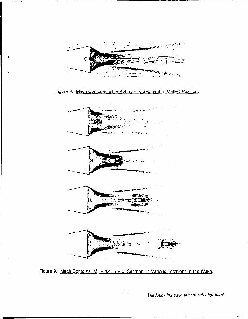
8. Mach Contours, M, = 4.4, a = 0, Segment in Matted Position ............. 21

9. Mach Contours, M_ - 4.4, a = 0, Segment in VariousLocations in the W ake ......................................... 21

10. Computed Pressure Contours for the EntireSystem , M_ = 4.4, a = 0 ....................................... 23

11. Comparison of Computed Pressure Contours With Spark Shadowgraph,M . -- 4.4, ax - 0 ............................................. 23

12. Drag Coefficient, M_ - 4.4, a - 0, (Static and Dynamic) ................ 25

13. Separation Distances Time, M. = 4.4. a = 0. (Dynamic) ................ 25

14. Segment Velocity vs Time, M_ = 4.4, a = 0, (Dynamic) ................. 26

v

INTENTIONALLY LEFT BLANK.

1. INTRODUCTION

An important parameter in the design of shell and bodies flying in relative motion to each other

is the total aerodynamic drag. The base drag constitutes a large part of the total a•;odynamic

drag and accurate prediction of the base region flow field is necessary. The ability to compute

the base region flow field for projectile configurations using Navier-Stokes computational

techniques has been developed over the past several years.1'2'3 Recently, improved numerical

predictions have been obtained by using the Cray-2 supercomputer and a more advanced zonal

upwind flux-split algorithm."'5 This zonal scheme preserves the geometry of the base corner

which allows an accurate modeling of the base region flow. Previous computational studies have

been completed showing the aerodynamic effect for a variety of base geometries. These

calculations, however, were performed on stand-alone projectile configurations and represent a

single-body problem. Recently a multibody problem which involves other bodies flying in the

wake of a parent projectile has required computational analyses. This is due in part to the

difficulty in finding good experimental and/or analytical data for such problems. The particular

problem here is to determine the aerodynamic effect of small cylindrical segments being ejected

into the wake of a parent projectile. The complexity and uniqueness of this problem results from

the trailing segments being in relative motion to each other, embedded in a non-uniform wake

flow, and requiring a time dependent solution. Figure 1 is a spark shadowgraph picture of a

recent range test 7 conducted with a number of segments flying in the wake of the parent

projectile. Computational results have been obtained by the authors for both the quasi-steady

case of fixed positions of the segments in the wake" and the dynamic case which involves time-

accurate numerical computations and is the subject matter of this technical report.

The time-accurate numerical simulation of the multiple aerodynamic bodies in relative motion

has been obtained using the Chimera9 approach. This technique has been used to compute

inviscid and viscous flows about complex configurations, 1 1'"2 and has been demonstrated for

unsteady viscous flow problems with bodies in relative motion. 3 The Chimera approach is a

domain decomposition method which uses overset, body-conforming grids and grew out of the

necessity to computationally model geometrically complex configurations. The originally developed

Navier-Stokes code, zonal F3D , was extended by the authors to include the details of the

Chimera procedure. This unique work couples the solution of the Navier-Stokes equations, which

govern fluid motion, with the solution to the six DOF (degree-of-freedom) equations of motion.

1

The coupling of the fluid dynamic solution and rigid body motion is a major advance and a

significant accomplishment which eliminates the need for simplifying assumptions and allows

more accurate physically based simulations.

2. GOVERNING EQUATIONS AND SOLUTION TECHNIQUE

The complete set of time-dependent, Reynolds-averaged, thin-layer Navier-Stokes equations

is solved numerically to obtain a solution to this problem. The numerical technique used is an

implicit, finite-difference scheme. Time-accurate calculations are made to numerically simulate

the ejection and separation of the segments in the wake of a parent projectile.

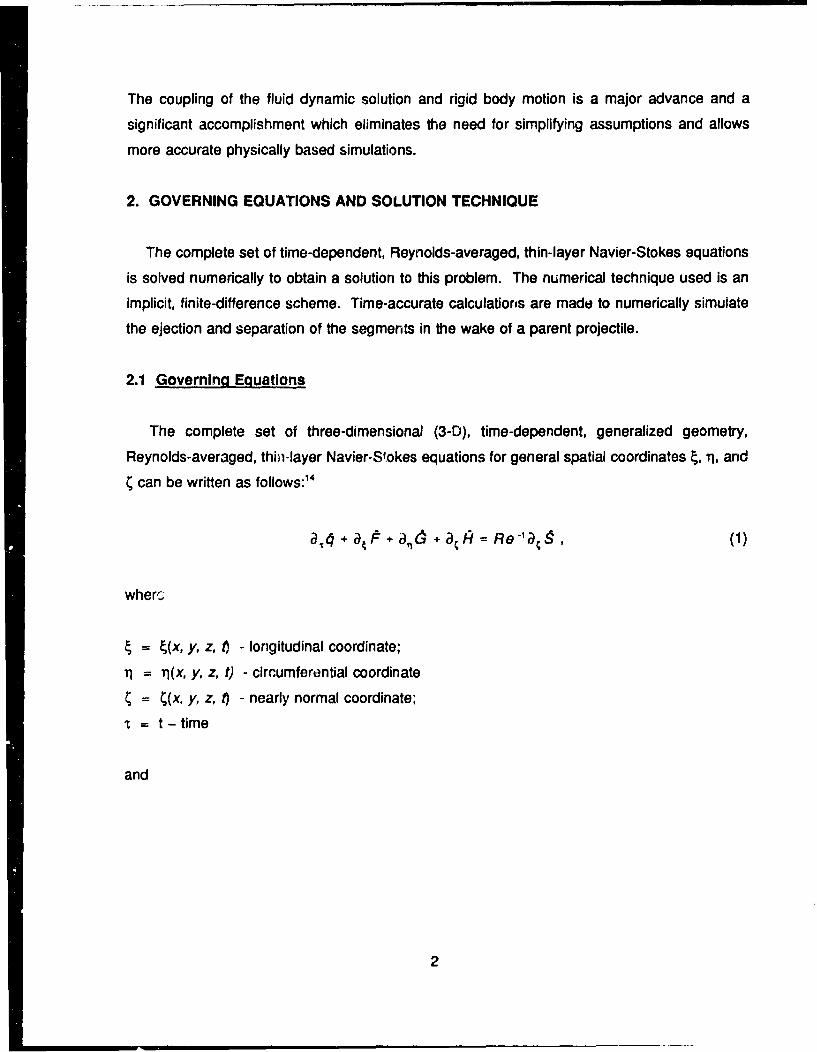
2.1 Governing Equations

The complete set of three-dimensional (3-D), time-dependent, generalized geometry,

Reynolds-averaged, thioi-layer Navier-Stokes equations for general spatial coordinates 4, rl, and

Scan be written as follows:14

a,4l + a,• 4P+ * arid ll Re-a..(1)

whero

S= ý(x, y, z, t• - longitudinal coordinate;

Tl = i1(x, y, z, t) - circumferential coordinate

S= C(x, y, z, t) - nearly normal coordinate;

,r = t - time

and

2

r

P p U

pu puU + p

pw pwU+4,

e jL(e+P) u -tlP

(2)

p V 1pWpuV + 11P puW + Cp

6=1 PVV +1P n- 1 pvW + yp

Pwv + ip pww + C~p

and where

0

A K, C' +ýZ)U; + L( ý,U + ýy;+

g 2+ ý2 + ý)Vt + _E(ý U + CV; + CW;) ý

C + C + CZ ) W 3 4( t,,U; + C C+ W

2+ 2+2[E U2 + V2+ W2); (3)

+ ic a, 1Pr(y -T 1

+ C, (,u + ýyv+ C',W)( U; + ý t+ C,~ }t3

3

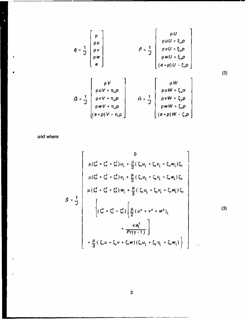
In Equation 1, the thin-layer approximation is used, and the viscous terms Involving velocity

gradients in both the longitudinal and circumferential directions are neglected. The viscous terms

are retained in the normal direction, C, for the projectile and segments, and are collected into the

vector 9. In the wake or the base region, similar viscous terms are also added in the streainwise

direction, •. For this computation, the diffusion coefficients p. and K contain

molecular and turbulent parts. The turbulent contributions are supplied through an algebraic eddy

viscosity turbulence model developed by Baldwin and Lomax.1'5

The velocities in the 4, T1, and ý coordinate directions can be written as

U 4t + A,+ % + ý

V = t + Uqx + Vy + wrIz

wI= + + +

which represent the contravariant velocity components.

The Cartesian velocity components (u, v, w) are retained as the dependent variables and are

nondimensionalized with respect to a_, (the free-stream speed of sound). The local pressure is

determined using the relation,

P (y - 1 )[e - 0.5p(u 2 + + w+)] (4)

where y is the ratio of specific heats. Density, p, is referenced to p, and the total

energy, e, to p_ a _2 . The transport coefficients are also nondimensionalized with respect to the

corresponding free-stream variables. Thus the Prandtl number which appears in 9 is defincd as

Pr = Cpj_//K..

2.2 Numerical Technique

The implicit, approximately factored scheme for the thin-layer Navier-Stokes equations using

central differencing in the T1 and ý directions and upwinding in , is written in the

following form,"6

4

I+ Ibh6(A*)" + ibh 6S•" - ih Re-J6J - iMD,I

x [I + ib a1 (A-)" + '•b' a11 -ibDII,],•A (6)

= ibAt{~(p ()f, - f.'4 + 8,'[( P-) - 'U-+ 8?,( cOn - e,.)

+ 68(" -W ) - Re-'(•" -n_.1)) - 0)O.( 6 - 6.)

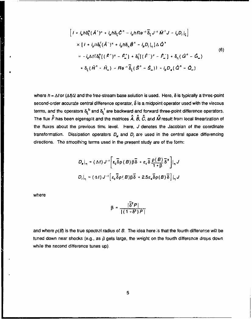
where h = Ator (AMf2 and the free-stream base solution is used. Here, 6 is typically a three-point

second-order accurate central difference operator, 8 is a midpoint operator used with the viscous

terms, and the operators atb and St' are backward and forNard three-point difference operators.A A A A A

The flux F has been eigensplit and the matrices A, B, C, and M result from local linearization of

the fluxes about the previous timc level. Here, J denotes the Jacobian of the coordinate

transformation. Dissipation operators De and D, are used in the central space differencing

directions. The smoothing terms used in the present study are of the form:

D.,n (A t) J-[,ýp(B) J'+ E-4 P ( )', J

0,! = (/At)J-'[ ep(e B)3 + 2.5e, ip(B)6j InJ

where

p = 1RPI

(1 t62)PI

and where p(B) is the true spectral radius of B. The idea here ;s that the fourth difference wikl be

tuned down near shocks (e.g., as i3 gets large, the weight on the fourth difference drops down

while the second difference tunes up).

5

2.3 Chimera Composlte Grid Stheme

The Chimera overset grid scheme is a domain decomposition approach where a configuration

is meshed using a collection of overset grids. It allows each component of the configuration to

be gridded separately and overset into a main grid. Overset grids are not required to join in anyspecial way. Usually there is a major grid which covers the entire domain or a grid generated

about a dominant body. Minor grids are generated about the rest of the other bodies. Because

each component grid is generated independently, portions of one grid may be found to lie within

the solid boundary contained within another grid. Such points lie outside the computational

domain and are excluded from the solution process.

Figures 2 and 3 show an example where tWe parent projectile grid is a major grid and the

segment grid is a minor grid. The segment grid is completely overlapped by the projectile grid:

thus, its outer boundary can obtain information by interpolation from the projectile grid. Similar

data transfer or communication is needed from the segment grid to the projectile grid. However,

a natural outer boundary tha•t overlaps the segment grid does not exist for the projectile grid.

The Chimera technique create,,,, an artificial boundary (also known as a hole boundary) within the

projectile grid which provides the required path for information transfer from the segment grid to

the projectile grid. The resulting hole region is excluded from the flow field solution in the

projectile grid. Equation 5 has been modified for Chimera overset grids by the introduction of the

flag i, to achieve just that. This i•, array accommodates the possibility of having arbitrary holes

in the grid. The ib array is defined such that it = 1 at normal grid points and 'b = 0 at hole points.

Thus, when i. = 1, Equation 5 becomes the standard scheme. But, when i, = 0, the algorithm

reduces to Ad" = 0 or d`1 = &, leaving d unchanged at hole points. The set of grid points

which form the border between the hole points and the normal field points are called intergrid

boundary points. These points are updated by interpolating the solution from the overset grid that

created the hole. Values of the ib array and the interpolation coefficients needed for this update

are provided by a separate algorithm."

In the present study, which involves multiple bodies in relative motion, the location of the holes

and the intergrid boundary points are time-dependent. Accordingly, the 'b array and the

interpolation coefficients are functions of time. This procedure of unsteady Chimera

decomposition has been successfully demonstrated by Meakin.' 3 The method depends on three

6

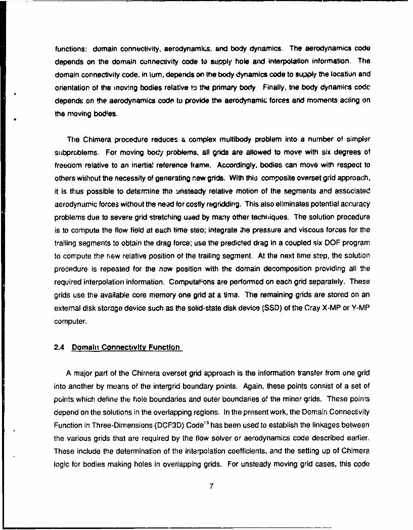
functions: domain connectivity, aerodynamics, and body dynamics. The aerodynamics code

depends on the domain connectivity code to supply hole and interpolation information. The

domain connectivity code. in turn, depends on the body dynamics code to supply the location and

orientation of the moving bodies relatve to the primary body Finally, the body dynamics code

depends on the aerodynamics code to provide the aerodynamic forces and moments acting on

the moving boc~es.

The Chimera procedure reduces & complex multibody problem into a number of simpler

s=•bproblems. For moving bod/ problems, all grids are allowed to move with six degrees of

freecom relative to an inertia! reference frame. Accordingly, bodies can move with respect to

others wiihout the necessity of generating new grids. With this composite overset grid approach,

it is thus possible to determine the unsteady relative motion of the segments and associated

aerodynamic forces without the nead for costly regridding. This also eliminates potential accuracy

problems due to severe grid stretching uaed by many other techuiiques. The solutior procedure

is to compute the flow field at each time steo; integrate the pressure and viscous forces for the

trailing segments to obtain the drag force; use the predicted drag in a coupled six DOF program

to compute the new relative position of the trailing segment. At the next time step, the solution

procedure is repeated for the now position with the domain decomposition providing all the

required interpolation information. Computations are performed on each grid separately. These

grids use the available core memory one grid at a tirna. The remaining grids are stored on an

external disk storage device such as the solid-state disk device (SSD) of the Cray X-MP or Y-MP

computer.

2.4 Domain Connectivity Function

A major part of the Chimera overset grid approach is the information transfer from one grid

into another by means of the intergrid boundary points. Again, these points consist of a set of

points which define the hole boundaries and outer boundaries of the minor grids. These points

depend on the solutions in the overlapping regions. In the present work, the Domain Connectivity

Function in Three-Dimensions (DCF3D) Code13 has been used to establish the linkages between

the various grids that are required by the flow solver or aerodynamics code described earlier.

These include the determination of the interpolation coefficients, and the setting up of Chimera

logic for bodies making holes in overlapping grids. For unsteady moving grid cases, this code

7

must be executed at (. Ach time iteration. To minimize the computation time, this code uses the

knowledge of hole and interpolated boundary points at time level n to limit its search regions for

finding their corresponding locations at time level n+1.

In general, vach component grid in an overset grid system represents a curvilinear system

ot points. However, the position of all points in all the grids are defined relative to an inertial

system of reference. To provide domain connectivity, inverse mappings are used which allow

easy conversion from x,y,z inertial system to 4,rý,T computational space. For moving body

problems, these maps for component grids are created only once. Identification of the intergrid

boundary points which correspond to the outer boundaries of the minor grids are done simply by

specifying appropriate ranges of coordinate indices. The rest of the intergrid boundary points

which result from holes created by a body in overset grids is a little more difficult to identify. A

collection of analytical shapes such as cones, cylinders, and boxes are used to cut holes in this

methed.

2.5 Boundary Conditions

For simplicity, most of the boundary conditions have been imposed explicitly.3 An adiabatic

wall boundary condition is used on the body surface, and the no-slip boundary condition is used

at the wall. The pressure at the wall is calculated by solving a combined momentum equation.

Free-stream boundary conditions are used at the inflow boundary as well as at the outer

boundary. A symmetry boundary condition is Imposed at the circumferential edges of the grid,

while a simple extrapolation is used zt th3 downstream boundary. A combination of symmetry

and extrapolation boundary condition is used at tV.e center line (axis). Since the free-stream flow

is supersonic, a nonreflection boundary condition is used at the outer boundary. Similar boundary

conditions are used for the segments.

3. MODEL GEOMETRY AND COMPUTATIONAL GRID

The primary or parent projectile is a 1 0-caliber (1 caliber = diameter at the cylindrical section)

cone-cylinder-flare projectile. It consist, of a 4.46-caliber conical nose, a 2.82-caliber cylindrical

section, and a 3.0-caliber 12.20 flare. Figure 4 shows a computational grid for this case. It shows

the projectile configuration and the surrounding grid which consists of approximately 20,000 grid

8

points. The grid in the wake region consists of 99 points in the streamwise direction and 119

points in the normal direction. The surface points for each region (body and wake) are selected

using an interactive design program. Each grid section was obtained separately and then

appended to provide the full grid. TPie grid for the body region, as well as the wake region, was

obtained algebraically. An expanded view of the wake region grid is shown in Figure 5. The

projectile afterbody seen here went through many design changes after the computations were

completed. This resulted in the use of a slightly different afterbody in the test firings compared

to the computational model afterbody. However, because of the relatively large size of the

afterbody base compared to the segment, the effect of this change in the afterbody is expected

to be minimal on the flow field over the segments. Figure 5 clearly shows the grid clustering near

the base corner of the projectile. Another unique feature of this grid is that the dark band of grid

points at the base corner (in the normal direction) slowly opens up with increasing distance

downstream of the base. This is an effort to make good use of the grid points and place them in

regions of large flow gradients such as the free shear layer in the wake region. The full grid is

split into five zones--a small zone in front of the projectile, three zones on the projectile itself, and

a wake zone.

The current problem of interest is the effect of the wake of the primary projectile on the small

cylindrical body. Each cylindrical segment has a diameter of 9 mm and a length to diameter ratio

(LID) of 2. A typical body conforming grid for the segment is shown in Figure 6 and is overset

onto the primary projectile grid. This corresponds to the matted position when the segment is

positioned inside of the parent projectile with the aft end of the segment flush with the base of

the parent projectile. The segment grid is generated easily independently of the major grid. It

consists of 101 points in the streamwise direction and 31 points in the normal direction away from

the body surface. The Chimera technique, as stated earlier, allows individual grids to be

generated with any grid topology, thus making the grid generation process easier. For moving

body problems, the segment grid, shown in Figure 6 in the matted position, moves with the

segment as the segment separates from the parent projectile and moves downstream into the

wake (see Figure 7). Again, there is no need to generate new grids for the segment and/or the

parent projectile during the dynamic process.

9

4. RESULTS

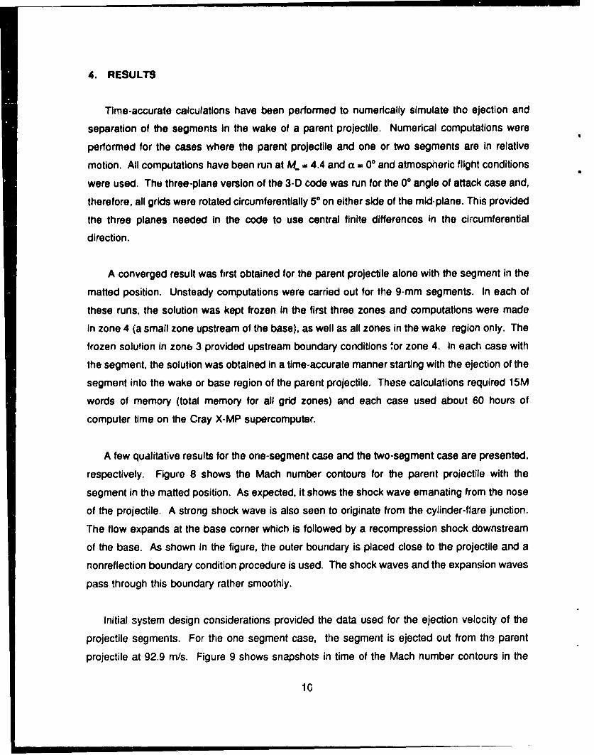
Time-accurate calculations have been performed to numerically simulate tho ejection and

separation of the segments in the wake of a parent projectile. Numerical computations were

performed for the cases where the parent projectile and one or two segments are in relative

motion. All computations have been run at MP - 4.4 and (x - 00 and atmospheric flight conditions

were used. The three-plane version of the 3-D code was run for the 00 angle of attack case and,

therefore, all grids were rotated circumferentially 50 on either side of the mid- plane. This provided

the three planes needed in the code to use central finite differences in the circumferential

direction.

A converged result was first obtained for the parent projectile alone with the segment in the

matted position. Unsteady computations were carried out for the 9-mm segments. In each of

these runs, the solution was kept frozen in the first three zones and computations were made

in zone 4 (a small zone upstream of the base), as well as all zones in the wake region only. The

frozen solution in zone 3 provided upstream boundary conditions for zone 4. In each case with

the segment, the solution was obtained in a time-accurate manner starting with the ejection of the

segment into the wake or base region of the parent projectile. These calculations required 15M

words of memory (total memory for all grid zones) and each case used about 60 hours of

computer time on the Cray X-MP supercomputer.

A few qualitative results for the one-segment case and the two-segment case are presented,

respectively. Figure 8 shows the Mach number contours for the parent projectile with the

segment in the matted position. As expected, it shows the shock wave emanating from the nose

of the projectile. A strong shock wave is also seen to originate from the cylinder-flare junction.

The flow expands at the base corner which is followed by a recompression shock downstream

of the base. As shown in the figure, the outer boundary is placed close to the projectile and a

nonreflection boundary condition procedure is used. The shock waves and the expansion waves

pass through this boundary rather smoothly.

Initial system design considerations provided the data used for the ejection velocity of the

projectile segments. For the one segment case, the segment is ejected out from the parent

projectile at 92.9 m/s. Figure 9 shows snapshots in time of the Mach number contours in the

10

base region for various locations of the segment in the wake. The first picture on the top of this

figure corresponds to the case when the segment has just come out of the base of the parent

projectile. The other three positions or locations correspond to separation distances (L) of about

2, 4, and 6 calibers from the base of the parent projectile. For L,-2, the segment is completely

immersed in the subsonic wake of the parent projectile. As seen In this figure, for L-4, the flow

right in front of the segment is still subsonic. The flow becomes supersonic away from it in the

normal direction and one can see the recompression shock which follows the flow expansions at

the base of the parent projectile. As the separation distance is increased to L=6, the flow field

ahead of the segment becomes supersonic. A bow shock wave forms ahead of the segment.

As L is increased further, this bow shock wave becomes stronger. These changes in the flow

structure change the pressure on the front face of the segment (stronger the shock, higher the

pressure) and thus, the aerodynamic drag. The overall flow field behind the segment looks

generally the same in all these cases and the pressure on the back face of the segment does not

change significantly.

A set of range tests7 have been performed for the multi-segment ejection case from the parent

projectile. Various configurations with different length-to-diameter ratios and nose radii of the

segment were included in the tests. The particular case for which numerical computations have

been made corresponds to a L./ of 2 and nose radius of 0.5 caliber. Two segments have been

numerically simulated. The ejection velocities for these two segments are 52 and 27 m/s for the

first (first one to come out) and second segment, respectively. The initial conditions used in the

numerical computations for ejection of these segments were obtained from the experimental test

results. The second segment was ejected after the first segment was about 1.9 calibers away

from the base of the parent projectile. The developed Chimera composite overset grid approach

was used to numerically model this experimental, tirne-dependent separation process. Figure 10

shows the computed pressure contours for the entire configuration which includes the parent

projectile and the two segments. It shows the instantaneous shock wave and the expansion

waves structure when the segments are about 4 and 10 calibers away in the wake. Comparison

of the computational results are made with the available experimental results. Figure 11 shows

the computed pressure contours in the base region for the two-segment case compared with the

experimentally obtained spark shadowgraphs. It corresponds to the case where the second

segment is at a separation distance of about 1.25 calibers from the base of the parent projectile.

At that time, the first segment is at a separation distance of about 3.8 calibers. As seen in the

11

figure. these locations agree well with the experimental test results. Although not shown here,

similar comparisons have also been made for other segment positions further downstream in the

wake indicating good agreement between the computed and experimental results.

The entire flow field over the projectile, including the segment, is computed to obtain the

desired aerodynamics. Surface pressures, including the base pressures and the viscous

stresses, are known from the computed flow field and can be integrated to give the aerodynamic

drag for both parent projectile as well as the cylindrical segments. The drag coefficient for the

segments is shown in Figure 12 as a function of the separation distance. This drag coefficient

is based on the area of the segment and the free-stream dynamic pressure. As mentioned

earlier, for small separation distances ( L<2 ), the segment is submerged in the subsonic wake

of the parent projectile. The pressure behind the segment is higher than the pressure ahead of

the segment and, therefore, results in negative drag. As L is increased, the approaching flow to

the segment becomes supersonic and a bow shock wave forms in front of the segment. This

increases the pressure at the front face of the segment and results in higher drag. Figure 12 also

shows the increase in drag with increasing separation distance. Also included here are the

previously computed6 quasi-static results obtained for a few locations of the segment in the wake

of the parent projectile. Thece calcu!ations do not take into account the relative motion between

the parent body and the segment. As seen in this figure, there is a substantial difference in the

predicted drag between the static and the dynamic cases with the drag being lower for the

dynamic case. This highlights the need for time-dependeni dynamic solution techniques to

accurately simulate problems involving multiple bodies in relative motion. The drag for the first

segment (first one to come out) is shown in solid line. For the first two calibers of separation

distance, both segments essentially follow the same curve. However, for L > 2.5, the drag of the

first segment is found to be lower than that of the second segment since it is in the wake of the

second segment. Although not shown here, the drag for the parent projectile changes very little

in the presence of the small cylindrical segments.

Figures 13 and 14 show the separation distance and the segment velocity as a function of

time, respectively. The computed result for the first segment is shown by the solid line and that

of the second one by a dashed line. The second segment is ejected about 1.2 ms after the first

one. As shown in Figure 13, the separation distance for the initial matted position of the

segments is -0.3 calibers. The computed locations of the segments agree fairly well with the

12

experimentally observed results. Figure 14 shows the comparison of the computed segment

velocity (relative to the parent projectile) with the data. For tho first 2 msec, the segment velocity

for the first segment decreases slightly and then increases from thereon with time. The segment

velocity for the second segment decreases only slightly during this time duration. Again, this

trend is seen in the experimental results as well.

5. CONCLUDING REMARKS

A computational study has been undertaken to compute the aerodynamics of small cylindrical

segments being ejected into the wake of a parent projectile. Flow field computations have been

performed at a supersonic Mach number, M. = 4.4 and a =0.00 using an unsteady, zonal F3D,

Navier-Stokes code and the Chimera composite grid discretization technique. The computed

results show the qualitative features of the base region flow field for the parent projectile for both

the matted position and other positions of the segment in the wake. The predicted flow field over

the small segmenis was found to undergo significant changes as the segments separated from

the parent projectile. For small separation distances (L<2), the segment experiences negative

drag for the dynamic case. With increasing separation distance, a bow shock was found to form

in front of the segment resulting in higher drag. A significant difference in the predicted drag was

observed between the quasi-steady and the dynamic simulations. The time-dependent

computations were shown to be essential for problems involving relative motion. Comparison of

the computed results for the two-segments case have been made with the available experimental

results and computed locations, separation distances, and segment velocities were found to be

in very good agreement with the experimental results.

This work represents a major advance in capability for determining the aerodynamics of

multiple-body configurations. The coupling of the fluid dynamic solution and rigid-body motion

is a major advance and significant accomplishment that eliminates the need for simplifying

assumptions and allows more accurate physically based simulations. Together with increased

computational resources and the advanced technologies described in this report, multiple design

configurations can be accurately simulated with a "best* design being chosen more quickly.

13

Figure 1. Spark Shadow-graph for Multiple Segments in Wake of the Parent Projectile.

14

PARENT(MAJOR) DOMAIN ARTIFICIAL BOUNDARY INPARENT DOMAIN

SEGMENT(MINOR) DOMAIN

Figure 2. Intergrid Communication.

SEGMENT BC CONDITIONINTERPOLATED FROMPARENT GRID

PARENT GRID

. ,, SURFACE IN SEGMENT GRID. THAT CREATES HOLE IN PARENT

S- GRID

OLE BOUNDARY INPARENT GRID

PARENT BC INTERPOLATEDFROM SEGMENT GRID

OVERLAP REGION

Figure 3. Overlap Region Between Grids.

15The following page intent onally left blank.

2477V L li 1

Figure 4. Computational Grid for the Parent Projectile (Major Grid).

-'-4- -414- - - ----

I-P

-7r

Figure 5. Expanded View of the Base Region Grid.

17The following page intentionally left blank.

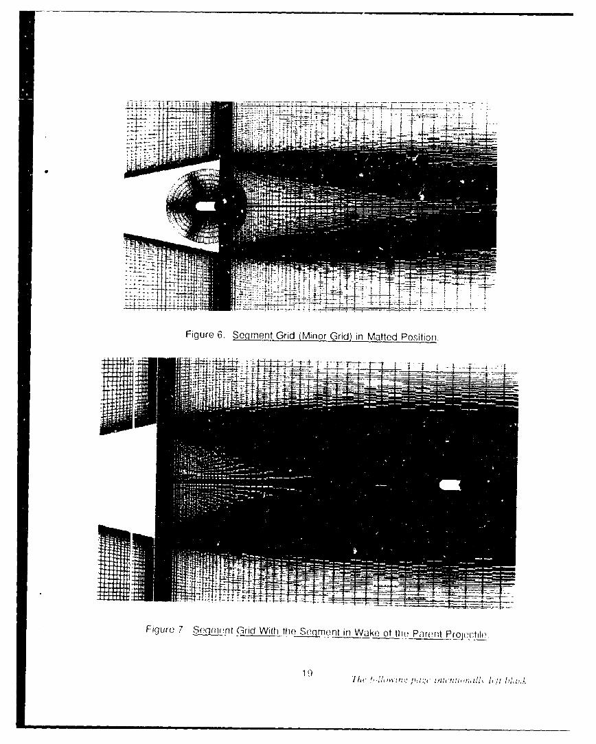
Figure 6. Segqment Grid (Minor, Grid) in Matted Position.

F gujru 7 Sogniriwt G-rid With theL S(n nt in Wake ot the, Parent Projectlk

C_

Figure 8. Mach Contours. M_ 4.4, q 0. Segment in Matted Position.

I.- -- z =

Figure 9. Mach ContoursM,--- 4.4, a - 0, Segqment in Various Locations in the Wake.

21 The following page intentionally left blank,

Figure 10. Computed Pressure Contours for the Entire System, M_ 4.,a 0

Figuie 11. Comnpari!ýon Of Compu~ted Pressure Contours, Wi -iSrk ShadowqaTh, M 4.4

(X0.

'3 'F/icfollowing pageý ifllf' fWllallv hfir blank

0.5

0.4 0 OUASI-STEADY03AMi ..F..ST S

CD 0.2

0.1

0. 0-oo-0. 1

0.0 2.0 4.0 6.0 8.0 10.0 12.0 14.0

L, Separation Distance (Calibers)

Figure 12. Drag Coefficient, M_ = 4.4. a = 0 (Static and Dynamic).

Q2 10.0•" 0F)COMP. (FIRST SEGMENT)-

-' 8.0 - 0 EXP. (FIRST SEGMENT)13 EXP. (SECOND SEGMENT)

(D 6.0 -C.Co+-# 4.0 - 0Co

-- 2 .0 . .. .. .......... . - .. -

0Co&.- 0.0

f -2.00.0 2.0 4.0 6.0 8.0 10.c

Time (millisec)

Figure 13. Separation Distance vs Time, M_ = 4.4. ot = 0 (Dynamic).

25

60.0 -S0

co 50.0 -E> 40.0

o 30.0"• "''"...... ".... '.. ......... "..... *......."........ •

" 20.0C- CO MLLPIR ST SEGMENT)

,- CQMP.(SEC)NDSEGMENTI

- 10.0 -0 EXP. (FIRS" SEGMENT).0 EXP. (SECOND SEhGMF.NT)

U)

0 .0 I 8 1 0 .0.0 2.0 4.0 6.0 8.0 10.0

Time (millisec)

Figure 14. Seamernt Velocity vs Tirme, M_ = 4.4. a = 0 (Dynamic).

20

6. REFERENCES

1. Sahu, J., C. J. Nietubicz, and J. L. Steger. "Navier-Stokes Computations of Projectile Base

Flow With and Without Base Injection." BRL-TR-02532, U.S. Army Ballistic Research Laboratory,

Aberdeen Proving Ground, MD, Novernber 1983 (also see AIAA Journal, vol. 23, no. 9,

pp. 1348-1355, September 1985).

2. Sahu, J. "Supersonic Base Flow Over Cylindrical Afterbodies With BAse Bleed." AIAA Paper

No. 86-0487, Proceedings of the 24th Annual Aerospace Sciences Meeting, Reno, NV, January

1986.

3. Sahu, J. "Computations of Supersonic Flow Over a Missile Afterbody Containing an Exhaust

Jet." AIAA Journal of Spacecraft and Rockets, vol. 24, no. 5, pp. 403-410, September-October

1987.

4. Sahu, J., and J. L.. Steger. "Numerical Simulation of Three-Dimensional Transonic Flows."

AIAA Paper No. 87-2293, Atmospheric Flight Mechanics Conference, Monterey, CA, August 1987

(also see BRL-TR-2903, March 1988).

5. Sahu, J. "Numerical Computations of Transonic Critical Aerodynamic Behavior." AIAA

Journal, vol. 28, no. 5, pp. 807-816, May 1990 (also see BRL-TR-2962, December 1988).

6. Sahu, J., and C. J. Nietubicz. "Three Dimensional Flow Calculation for a Projectile With

Standard and Dome Bases." BRL-TFI-3150, U.S. Army Ballistic Research Laboratory, Aberdeen

Proving Ground, MD, September 1990.

7. Von Wahlde, R. Private Communications, Army Research Laboratory.

8. Sahu, J. , and C.J. Nietubicz. "A Computational Study of Cylindrical Segments in the Wake

of a Projectile." BRL-TR-3254, U.S. Army Ballistic Research Laboratory, Aberdeen Proving

Ground, MD, August 1991.

27

9. Steger, J.L., F.C. Dougherty, and J.A. Benek. "A Chimera Grid Scheme.t ,Advances In Grid

Generation, K.N. Ghla and U. Ghla, eds., ASME FED-5, June 1983.

10. Atta, E.H., and J. Vadyak. "A Grid Interfacing Zonal Algorithm for Three-Dimensional Flow

Transonic Flows about Aircraft Configurations." AIAA Paper No. 82-1017, 1982.

11. Benek J.A., T.L. Donegan, and N.E. Suhs. "Extended Chimera Grid Embedding Scheme

with Application to Viscous Flows." AIAA Paper No. 87-1126-CP, 1987.

12. Buning, P.G., I.T. Chiu, S. Obayashi, Y.M. Rizk, and J.L. Steger. "Numerical Simulation of

the Integrated Space Shuttle Vehicle in Ascent." AIAA Atmospheric Flight Mechanics Conference,

August 15-17, 1988.

13. Meakin, R.L., and N. Suhs. "Unsteady Aerodynamic Simulation of Multiple Bodies in Relative

Motion." AIAA 9th Computational Fluid Dynamics Conference, AIAA Paper No. 89-1996, June

1949.

14. Pulliam, T. H., and J. L. Steger. "On Implicit Finite-Difference Simulations of

Three-Dimensional Flow." AIAA Journal, vol. 18, no. 2, pp. 159-167, February 1982.

15. Baldwin, B, S., and H. Lomax. "Thin Layer Approximation and Algebraic Model for Separated

Turbulent Flows." AIAA Paper No. 78-257, January 1978.

16. Steger, J.L., S.X. Ying, and L.B. Schiff. "A Partially Flux-Split Algorithm for Numerical

Simulation of Compressible Inviscid and Viscous Flows." Proceedings of the Workshop on

Computational Fluid Dynamics, Institute of Nonlinear Sciences, U. of California, Davis, CA, 1986.

28

No, of No, of.qg!II Q2iLaion .Q.9.e. Oroanization

2 Administrator 1 CommanderDefense Technical Info Center U.S. Army Missile CommandATTN: DTIC-DDA ATTN: AMSMI-RD-CS-R (DOC)Cameron Station Redstone Arsenal, AL 35898-5010Alexandria, VA 22304-6145

S1 CommanderCommander U.S. Army Tank-Automotive CommandU.S. Army Materiel Command ATTN: AMSTA-JSK (Armcr Eng. Br.)

* ATrN: AMCAM Warren, MI 48397-50005001 Eisenhower Ave.Alexandria, VA 22333-0001 1 Director

U.S. Army TRADOC Analysis CommandDirector ATTN: ATRC-WSRU.S. Army Research Laboratory White Sands Missile Range, NM 88002-5502ATTN: AMSRL-OP-SD-TA,

Records Management I Commandant2800 Powder Mill Rd. U.S, Army Infantry SchoolAdelphi, MD 20783-1145 ATTN: ATSH-WCB-O

Fort Benning, GA 31905-50003 Director

U.S. Army Research LaboratoryATTN: AMSRL-OP-SD-TL, Aberdeen Provina Ground

Technical Library2800 Powder Mill Rd. 2 Dir, USAMSAAAdelphi, MD 20783-1145 ATTN: AMXSY-D

AMXSY-MP, H. CohenDirectorU.S. Army Research Laboratory 1 Cdr, USATECOMATTN: AMSRL-OP-SD-TP, ATTN: AMSTE-TC

Technical Publishing Branch2800 Powder Mill Rd. 1 Dir, USAERDECAdelphi, MD 20783-1145 ATTN: SCBRD-RT

2 Commander I Cdr, USACBDCOMU.S. Army Armament Research, ATTN: AMSCB-CII

Development, and Engineering CenterATTN: SMCAR-TDC 1 Dir, USARLPicatinny Arsenal, NJ 07806-5000 ATTN: AMSRL-SL-I

Director 5 Dir, USARLBenet Weapons Laboratory ATTN: AMSRL-OP-AP-LU.S. Army Armament Research,

Development, and Engineering CenterATTN: SMCAR-CCB-TLWatervllet, NY 12189-4050

DirectorU.S. Army Advanced Systems Research

and Analysis Office (ATCOM)ATTN: AMSAT-R-NR, M/S 219-1Ames Research CenterMoffett Field, CA 94035-1000

29

No. of No. of

HODA (SARD-TR/Ms. K. Kominos) 1 USAF Wright Aeronautical LaboratoriesWASH DC 20310-0103 ATTN: AFWAL/FIMG, Dr. J. Shang

WPAFB, OH 45433-8553

HODA (SARD-TR/Dr. R. Chait)

WASH DC 20310--0103 DirectorNational Aeronautics and Space Administratior

5 Comamamtr Langley Research CenterI.S. Amniy .Amament Research, ATTN: Tech Library

Devc !op,trnordt, •nd Engineering Center Dr. M. J. HemschA'TrN: SMC;R-AET-A, Dr. J. Smith

H. H-udgins Langley StationS. Kahn Hampton, VA 23665J. GrauC. Ng 3 DirectorW. Koenig National Aeronautics and Space Administration

Picatinny Arsenal, NJ 07806-5000 Ames Research CenterATTN: MS-227-8, L. Schiff

Commander MS-258-1,U.S. Army Armament Research, T. Hoist

Development, and Engineering Center D. ChausseeATTN: SFAE-FAS-SD, M. Devine Moffett Field, CA 94035Bldg. 171Picatinny Arsenal, NJ 07806-5000 1 Massachusetts Institute of Technology

ATTN: Technical LibraryCommander 77 Massachusetts Ave.U.S. Army Missile Command Cambridge, MA 02139ATTN: AMSMI-RD-SS-AT, B. WalkerRedstone Arsenal, AL 35898-5010 2 Director

Sandia National LaboratoriesCommander ATTN: Dr. W. OberkampfU.S. N3val Surface Warfare Center Dr. F. BlottnerDahlgren Division Division 1554ATTN: Dr. F. Moore P.O. Box 5800Dahlgren, VA 22448 Albuquerque, NM- 87185

3 Commander 2 VRA Inc.Naval Surface Warfare Center ATTN: Dr. C. LewisATTN: Code R44, Dr. B. A. Bhutta

Dr. F. Priolo P.O. Box 50Dr. A. Wardlaw Blacksburg, VA 24060

K24, B402-12, Dr. W. YantaWhite Oak Laboratory 1 Science Applications, Inc.Silver Spring, MD 20903-5000 Computational Fluid Dynamics Division

ATTN: Dr. D. W. Hall3 Air Force Armament Laboratory 994 Old Eagle School Road

ATTN: AFATL/FXA, Suite 1018Dr. L. B. Simpson Wayne, PA 19087Dr. David BelkDr. G. Abate

Eglin AFB, FL 32542-5434

30

No, of No. ofCoDles OrgnigU Copies

6 Alliant Techsystems, Inc. 1 Florida Atlantic UniversityATTN: J. Bode Depaitment of Mechanical Engineering

C. Candland ATTN: Dr. W. L. ChowL. Osgood Boca Raton, FL 33431R. BurettaR. Becker 1 North Carolina State UniversityM. Swenson Department of Mechanical and Aerospace

600 Second St. NE EngineeringHopkins, MN 55343 ATTN: Prof. D. S. McRae

Box 7910McDonnell Douglas Missile Systems Co. Raleigh, NC 27695-7910ATTN: F. McCotterMallcode 306-4249 1 Georgia Institute of TechnologyP.O. Box 516 School of Aerospace EngineeringSt. Louis, MO 63166-0516 ATTN: Dr. Warren C. Strahle

Atlanta, GA 303322 Institute of Advanced Technology

ATTN: Dr. T. Kiehne 2 University of Illinois at Urbana-ChampaignDr. W. G. Relneke Department of Mechanical and Industrial

4030-2 W. Baker Lane EngineeringAustin, TX 78759 ATTN: Prof. A. L. Addy

Prof. Craig DuttonUniversity of California, Davis 114 Mechanical Engineering BuildingDepartment of Mechanical Engineering 1206 West Green StreetATTN: Prof. H. A. Dwyer Urbana, IL 61801Davis, CA 95616

1 Scientific Research AssociatesUniversity of Maryland ATTN: Dr. Richard BuggelnDepartment of Aerospace Engineering 50 Nye RoadATTN: Dr. J. D. Anderson, Jr. P.O. Box 1058College Park, MD 20742 Glastonbury, CT 06033

University of Texas 1 AEDCDepartment of Aerospace Engineering Calspan Field Service

and Engineering Mechanics ATTN: Dr. John BenekATTN: Dr. D. S. Dolling MS 600Austin, TX 78712-1055 Tullahoma, TN 37389

University of Florida 1 Visual ComputingDepartment of Engineering Sciences ATIN: Jeffrey 0. CordovaCollege of Engineering 883 N. Shoreline Blvd.ATTN: Prof. C. C. Hsu Suite B210Gainesville, FL 32611 Mountain View, CA 94043

Pennsylvania State University 1 MDA Enginoering, Inc.Department of Mechanical Engineering ATTN: John P. Steinbrenner

ATTN: Dr. Kenneth Kuo 500 E. Border St.University Park, PA 16802 Suite 401

Arlington, TX 76010

31

No. of No. ofCopies O~a~j7Aton Qol• Oroanlzation

Climate Control Division Aberdeen Provin GroundProduct Engineering OfficeAVTN: 'Tom Gielda 25 Dir, USARL15031 South Commerce Dr. ATTN: AMSRL-WT-P, Mr, Albert HorstDeartbom, MI 48120 AMSRL-WT-PB,

Dr. E. SchmidtCarrier Corporation Dr. M. BundyATTN: Howard Gibeling Dr. K. FanslerP.O. Box 4808 Mr. E. FerryCarrier Parkway Mr. B. GuldosSyracuse, NY 13221 Mrs. K. Heavey

Mr. H. EdgeNASA Marbhall Space Flight Control Center Dr. G. CooperATTN: Kevin Tucker Mr. V. OskayMail Stop ED-32 Dr. P. PlostinsHuntsville, AL 35812 Dr. A. Mikhail

Dr. J. SahuAerojet Electronics Plant Mr. P. WeInachtATTN: Dr. Dan Pillasch AMSRL-WT, Dr. A. BarrowsBldg. 170/Dept. 5311 AMSRL-WT-PD, Dr. B. BumsP.O. Box 296 AMSRL-WT-PA,Azusa, CA 91702 Dr. T. Minor

Mr. M. NuscaAMSRL-WT-W, Dr. C. MurphyAMSRL-WT-WB, Dr. W. D'AmicoAMSRL-WT-NC,

Ms. D. HisleyMr. R. Lottero

AMSRL-CI-C,Dr. W. SturekDr. N. Patel

AMSRL-CI-AD, Mr. C. Nietubicz

2 Cdr, USAARDEC,ATTN: Firing Tables, Bldg 120,

Mr. R. LieskeMr. R. McCoy

32

USER EVALUATION SHEET/CHANGE OF ADDRESS

This Laboratory undertakes a continuing effort to improve the quality of the reports it publishes. Yourcomments/answers to the items/questions below will aid us In our efforts.

I. ARL Report Number ARL-TR-590 Date of Report October 1994

2. Date Report Received

3. Does this report satisfy a need? (Comment on purpose, related project, or other area of interest for

which the report will be used.)

4. Specifically, how is the report being used? (Information source, design data, procedure, source of

ideas, etc.)

5. Has the information in this report led to any quantitative savings as far as man-hours or dollars saved,

operating costs avoided, or efficiencies achieved, etc? If so, please elaborate.

6. General Comments. What do you think should be changed to improve future reports? (Indicatechanges to organization, technical content, format, etc.)

Organization

CURRENT NameADDRESS

Street or P.O. Box No.

City, State, Zip Code

7. If indicating a Change of Address or Address Correction, please provide the Current or Correct addressabove and the Old or Incorrect address below.

Organization

OLD NameADDRESS

Street or P.O. Box No.

City, State, Zip Code

(Remove this sheet, fold as indicated, tape closed, and mail.)(DO NOT STAPLE)