QNET-CFD WIKI KNOWLEDGE BASE

APPLICATION CHALLENGE

PARTICLE-LADEN SWIRLING FLOW

Prof. Dr.-Ing. Martin Sommerfeld

Zentrum für Ingenieurwissenschaften Martin-Luther-Universität Halle-Wittenberg

D-06099 Halle (Saale), Germany Tel.: 0049-3461-4628-79; Fax: 0049-3461-4628-78

Martin.Sommerfeld@iw.Uni-Halle.de http://www-mvt.iw.uni-halle.de

APPLICATION CHALLENGE DOCUMENT

1. DESCRIPTION

1.1 INTRODUCTION

The special features of swirling flows are utilised in combustion systems in order to provide flame stabilisation and good mixing between fuel and oxidiser. This is achieved by the central recirculation bubble developing in front of the burner exit. Swirl burners are usually operated with liquid (spray) or pulverised fuels. In order to obtain a better understanding of the particle behaviour in such a complex swirling flow, detailed experiments were conducted on particle-laden swirling flow emanating into a pipe expansion (Sommerfeld and Qiu 1991). The gas-particle mixture was injected centrally without swirl together with a co-flowing swirling annular gas jet yielding a swirl number of about 0.5. Downstream of the inlet simultaneous measurements of gas and particle velocities (all three components) were conducted by phase-Doppler anemometry, which also provided local particle size distributions and the stream-wise particle mass flux. Two cases with different injection flow rates, but roughly identical swirl number were considered. Both cases showed a closed central recirculation region. Inlet conditions are available from highly resolved profiles 3 mm downstream of the edge of the inflow tubes. Since the particle mass loading is rather small two-way coupling effects are of minor importance. Numerical computations performed with the finite-volume code FASTEST in connection with the k-ε turbulence model showed reasonable good agreement with the measurements (Sommerfeld and Qiu 1993). The particle phase was simulated by Lagrangian tracking also yielding a quite good agreement with measured velocity profiles, the particle mass flux and the number mean particle diameter.

1.2 RELEVANCE TO INDUSTRIAL SECTOR

Particle- or droplet-laden swirling gas flows are found in numerous technical applications. In spray or coal fired combustion systems, swirling flows are used to establish very high mixing rates between fuel and swirling air stream and to ensure the required flame stability. This is achieved by the developing central recirculation region, where the hot reaction products are convected backward and mix with the fresh fuel and air. In addition particle-laden swirling flows are found in numerous different types of particle separation devices, such as air cyclones. The considered basic flow configuration allows detailed validation of computations for particle-laden swirling flows, especially with respect to Reynolds-stress turbulence modelling or LES applications and particle dispersion in anisotropic turbulence.

1.3 DESIGN OR ASSESSMENT PARAMETERS

The assessment parameters for this test case are the mean velocity profiles as well as those for the rms values along the test section for both phases. Additionally, profiles of the stream-wise particle mass flux could be estimated from the measurements revealing the centrifuging effect of a swirling flow. From the numerical calculations also the particle residence time as a function of particle size may be used to assess the performance of numerical calculations.

1.4 FLOW DOMAIN GEOMETRY

The swirling flow was realized in a kind of pipe expansion flow (Figure 1). Through the central inlet tube the gas-particle mixture was injected into the test section without swirl (outer diameter 32 mm). The co-flowing swirling flow was produced by a vane-swirl generator located upstream the inlet. The annular inlet tube has an inner diameter of 38 mm and an outer diameter of 64 mm. The test section has a diameter of 194 mm and a length of 1,500 mm. The end of the test section is connected to a sufficiently wide stagnation chamber.

Figure 1: Swirl Flow test section made from Plexiglas including the main dimensions (length 1,500 mm).

1.5 FLOW PHYSICS AND FLUID DYNAMICS DATA

The considered swirling flow is highly turbulent, but may be considered as incompressible. The measurements were done under ambient conditions with a temperature of about 300 K yielding a air density of 1.18 kg/m3 and a dynamic viscosity of 18.4·10-6 kg/(m·s). The characteristic non-dimensional parameters are: The flow Reynolds number which is calculated with the total volume flow rate, the outer diameter of the annulus and the effective inlet cross-sectional area Ain:

in

3

AµQDReρ

=

The swirl number which is the ratio of the axial flux of annular momentum to the axial flux of linear momentum obtained by integration across the primary and annular inlets:

∫∫

ρ

ρ= 2/D

0

25

2/D

0

2

3

3

drrUD

drUrW2S

Here U and W are the mean axial and tangential velocities and r is the radius. The values of the outer diameter of the inlet, D3, and the inner diameter of the test section D5 are given in

Fig. 1. The Reynolds numbers of the two cases considered are 52400 and 54500 and the swirl numbers are around 0.5. As mentioned above, the particle mass loading was rather low so that the effect of the particles on the flow field may be neglected. The particles are spherical glass beads with a material density of 2,500 kg/m3 and a relative wide size distribution ranging between about 10 µm to 80 µm. The number mean diameter is 45 µm yielding a mean Stokesian response time of about 15 ms.

µ

ρ=

18D

St2pp

Hence, the small particles in the spectrum will be able to respond to the turbulent fluctuations. However, with increasing particle size centrifuging effects become more and more important (see Sommerfeld and Qiu 1993).

2. TEST DATA

2.1 DESCRIPTION OF TEST CASE EXPERIMENTS

For the detailed study of particle-laden, swirling two-phase flows, a vertical test section with downward flow was chosen (Figure 2). In order to allow good optical access, a simple pipe expansion was selected as test section. Such a configuration has the advantage that the inlet conditions can be measured easily, which is important for performing numerical calculations. The complete test rig consists of two flow circuits (Figure 1) for the primary (6) and secondary annular flows (5), respectively. A blower (1) with a variable flow rate supplies these two pipe systems via a T-junction and a throttle valve (2) is used to adjust the flow rate at the primary inlet. The mass flow rates through the primary and annular inlets were obtained from two orifice flow meters (3). The secondary flow circuit is split into four smaller pipes which are connected radially to the swirl generator. The upper part of the swirl generator is constructed as a settling chamber, and the air passes over a number of screens and then moves radially inward across the radial swirl vanes. The swirl intensity of the annular flow may be adjusted continuously by turning the swirl vanes in the radial swirl generator (8). The primary flow circuit is connected to a pipe passing straight through the centre of the swirl generator. The dust particles are injected into the primary flow above the swirl generator by a particle feeder (4) with a variable-speed motor. Above the particle feeder, a reservoir (7) for the dust particles is installed. The inlet configuration and the dimensions of the test section are shown in Figure 1. The test section consists of a 1.5 m long Plexiglas tube with an inner diameter of 194 mm. The end of the test section is connected to a stagnation chamber (11). As a result, an annular type of central recirculation bubble was established in the upper part of the test section.

Figure 2: Overview of the swirl Flow test facility The stagnation chamber is connected to a cyclone separator (13) and an additional paper filter to separate both the large dispersed phase particles and the seeding particles, which are used as tracers for measuring the gas velocity. These tracer particles are injected into both pipe systems before the swirl generator. To guarantee that the flow rate in the test section is independent of the pressure loss in the filter system, which may vary during the measurements, an additional blower (12) is used in connection with a bypass valve at the stagnation chamber (11).

2.2 MEASUREMENT TECHNIQUE

Particle size and velocity measurements were performed at several cross-sections within the test section, including the inlet using a one-component PDA (phase-Doppler anemometer). Details on the configuration of the applied PDA-system can be found in Sommerfeld and Qiu (1991 and 1993). In order to allow measurements of all three velocity components (axial velocity u, radial velocity v, and tangential velocity w), the PDA system could be rotated and was mounted on a stepper-motor-controlled three-dimensional traversing system (Figure 1). The receiving optics was always mounted at an angle of 30° from the forward scattering direction. To avoid strong laser-beam deflections and a realignment of the receiving optics for every measuring point, the Plexiglas test section had several slits which were covered from

the inside by 100 µm thick glass plates. This results in negligible beam distortion, especially when the radial and axial velocities are measured, where the receiving optics have to be mounted in such a way that the optical axis of the receiving optics is oblique to the walls of the test section. For each velocity component, different test sections with different slit locations were used, which allowed the appropriate installation of the PDA receiving optics and the measurement of particle size-velocity correlation for each velocity component. In order to allow simultaneous measurements of gas and particle velocities, the flow was additionally seeded with small, spherical tracer particles (Ballotini, type 7000). This seeding was injected into both the primary and the annular jets far upstream the inlet to the test section. Since the size distribution of the particles ranges up to about 10 µm, a phase discrimination procedure was employed which insured that only tracer particles up to a maximum of 4 µm are sampled for determining the gas velocity. This procedure resulted in a measured mean diameter of about 1.5 µm for the validated signals from the tracer particles. A detailed description of the phase discrimination procedure was given previously by Sommerfeld and Qiu (1991). The particle mass flux was measured separately with the single-detector receiving system. The receiving optics was positioned 90° off-axis from the forward scattering direction in order to obtain an exact demarcation of the measuring volume. At each measuring point, the number of particles N traversing the control volume was counted within a certain time period ∆t, and the particle velocity was measured simultaneously. For these measurements the transient recorder was also operated in the sequential mode, which ensured a real-time data acquisition, at least for the particle concentrations considered. During the storage of the 400 events, an internal clock was used to determine the effective measuring time. The total particle mass flux is then obtained with the cross-section of the control volume Ac, which was calculated from the optical configuration:

c

pp At

mNf∆

=

where N, ∆t and pm are the counted number of particles, the total measuring time and the mean particle mass, respectively. The mean particle mass at a certain measuring location was calculated from the volume mean particle diameter obtained from the PDA size measurements. Due to the uncertainties in the determination of the cross-section of the control volume, the measured mass flux was corrected using the global mass balance. The total measured particle mass flow rate was obtained by integrating the mass flux profile at the inlet. In comparison with the global mass flow rate obtained by weighting the particles collected during a certain time period in the cyclone separator, a correction factor was determined and applied to the mass flux measurements at all other cross-sections. The integration of the measured and corrected mass flux profiles revealed that the error in the particle mass flow rate was in the range ± 20 % for the various profiles. This rather large error was caused mainly by the poor resolution of the measurements in the near-wall region, where the integration area is the largest in the circular cross-section of the pipe. Furthermore, the particle mass flux was separated to give the positive and negative fluxes, which gives additional information about the mass and number of particles having negative velocities. For this separation, the particle volume mean diameter for particles with only positive and negative axial velocity was determined from the PDA measurements. Measurements of the three velocity components were conducted at 8 cross-sections downstream of the inlet (i.e. 3, 25, 52, 85, 112, 155, 195 and 315 mm). At each measuring location, 2000 samples were taken to obtain the gas velocity and the associate rms. values. In

order to achieve reasonably accurate velocity statistics for the particle phase in the different size classes, 18,000 samples were acquired. The total measuring time for each location was between 15 – 30 min, which was strongly dependent on the local particle concentration. The maximum measurable particle size range, between 0 – 123.8 µm, was resolved by 40 classes, each 3.1 µm in width. Besides the information on the change in the particle size distribution throughout the flow field, the stored data of particle size and velocity could be reprocessed after the measurement in order to give the particle mean velocity in certain size classes.

2.3 MEASUREMENT ERRORS

Since the three velocity components were measured with a single component PDA-system the measurement errors are very small; i.e. less than about 5 %. For the measurement of the gas-phase velocity small spherical tracer particles were added. For identifying accurately the tracer signals a maximum phase angle was set whereby it was guaranteed that the tracer particles were smaller than about 3 µm (Sommerfeld and Qiu 1991). Such particles are able to follow the fluctuations of the gas flow. To determine the gas phase mean and rms velocities 2000 signals were collected. Errors in particle sizing may occur due to fluctuations in the phase size relation, especially for particles smaller than about 50 µm (Sommerfeld and Tropea 1999). Additional errors may be caused by the so-called trajectory ambiguity. These errors are however difficult to specify. Since for the particle phase 20,000 signal pairs were collected at each measurement location, the obtained size distributions were reasonable smooth. Therefore, the derived mean particle diameter should have an error of around ± 5 %. The measured size-velocity correlations are also very smooth for the major part of the size distribution around the modal value. Only near the edges of the size distribution with a lower number of samples some fluctuations are observed (Sommerfeld and Qiu 1991). The procedure for measuring the particle mass flux and the associated errors are discussed in the previous section.

2.4 FLOW AND INLET CONDITIONS

In the present experiments, two flow conditions with different flow rates at the particle-laden primary inlet were considered. The resulting maximum gas velocities in the primary jet for the two cases were 12.5 and 7.4 m/s, respectively. The flow rate in the annular inlet was adjusted to give a maximum velocity of about 18 m/s. The maximum tangential velocity was for both cases about 13 m/s, corresponding to a swirl vane angle of 30°. The resulting swirl number was about 0.5 in both cases. The associated mass flow rates for the gas and the particles, the flow Reynolds number, the swirl number and other experimental conditions are listed in Table 1. The mass flow rates of the primary and secondary annular jets were calculated from the pressure drops across the orifice flow meters. The flow Reynolds number was obtained with the total volume flow rate at the inlet and the outer diameter of the annulus (D3 = 64 mm). The swirl number was calculated as the ratio of the axial flux of angular momentum to the axial flux of linear momentum, which was obtained by integration across both the primary and annular inlets. Furthermore, the particle mass flow rates and the properties of the glass beads are given in Table 1. The particles have a smooth surface and are spherical in shape. Only less than about 2 % of particles were non-spherical or fragments, which resulted in small errors in sizing the beads by the PDA. Such a particle material is ideal for PDA studies in particulate two-phase-

flows. The particle size distribution obtained by a PDA measurement (18,000 samples) is given in Figure 3. Since during the experiment some of the smaller particles were not collected in the cyclone separator but were collected in the paper filter, the particle material was frequently renewed in order to guarantee that the particles always have the same size distribution. This was ensured by measuring the particle size distribution at the inlet from time to time. The effects of particle damage could not be observed in the present measurements.

Table 1. Flow conditions and particle properties Case 1 Case 2 Air flow Gas temperature [K] 300 300 Gas density [kg/m3] 1.18 1.18 Dynamic viscosity [kg/(m s)] 18.4

10-6 18.4 10-6

Mass flow rate of the primary jet [g/s]

9.9 6.0

Mass flow rate of the secondary jet [g/s]

38.3 44.6

Inlet Reynolds number (with D3 = 64 mm)

52400 54500

Swirl number 0.47 0.49 Particle phase Particle mass flow rate [g/s] 0.34 1.0 Particle loading in the primary jet 0.034 0.17 Particle properties Particle number mean number [µm] 45 Particle material density [kg/m3] 2500 Stokesian particle response time [ms] 15.2 Refractive index 1.52

Figure 3: Measured number based size distribution of the spherical glass beads at the inlet to the test section (number mean diameter 45 µm)

2.5 MEASURED DATA

Experiments were conducted for two swirl flow cases (Table 1). For each of the case the inlet data (at z = 3 mm) and the profiles at cross-sections 25, 52, 85, 112, 155, 195 and 315 mm downstream of the inlet are collected by traversing the PDA in steps between 5 and 10 mm, except for the inlet which was scanned at a higher resolution (between 1 and 3 mm). All the data for the two cases are available at: http://www-mvt.iw.uni-halle.de/testfaelle/swirldata. These data sets (SWCASE1 and SWCASE2) include profiles for the gas phase velocities (all three velocity components) and profiles of particle phase properties averaged over all particle size classes (three velocity components, stream-wise particle mass flux and particle number mean diameter as well as its rms values). Moreover, profiles of the mean velocities of three particle size classes, namely 30, 45 and 60 µm, are provided.

2.6 OVERVIEW OF EXPERIMENTAL RESULTS

The swirling flow structures established in the experiments exhibit closed central recirculation bubbles just downstream of the inlet and a rather short recirculation at the edge of the pipe expansion. Due to the strong spreading of the swirling jet, the reattachment length is considerably shorter than that for a similar pipe expansion flow without swirl. An overview of the gas flow field and the particle behaviour in the two swirl flow conditions considered (cases 1 and 2) is given in Figure 4, where the gas-phase zero axial velocity lines, the dividing streamlines and the zero axial velocity lines for the particles (averaged over all particle classes) are shown. The width of the central recirculation bubble is almost identical for both cases, whereas the length is larger for case 2. As a result of the lower axial momentum of the primary jet in case 2, the recirculation bubble moves closer to the inlet. The slightly higher swirl number in this case also gives rise to a shorter reattachment length of the recirculation region at the edge of the pipe expansion, as compared with case 1. The area of negative axial particle velocity exhibits an annular shape ranging from about 50 to 200 mm downstream of the inlet for swirl case 1. In case 2, where the particle initial momentum is lower, the particles have longer residence times in the flow and, therefore, respond faster to the flow reversal in the central recirculation bubble. The resulting area of negative particle axial velocities becomes wider and extends from 50 to about 250 mm in the stream-wise direction. The measurements of the cross-sectional profiles for the mean gas and particle velocities, the velocity fluctuations and the development of the particle mass flux and the particle number mean diameter reveal the particle response and dispersion characteristics. The measurements of the particle mass flux for the two flow situations already show considerable differences (Figure 5). The maximum of the mass flux near the centreline remains up to 200 mm downstream of the inlet for case 1. While in case 2, the particles begin to accumulate near the wall quite early (from z = 112 mm), and the maximum of the mass flux appears near the centreline only up to about z = 112 mm. Furthermore, it may be seen that the recirculating particle mass (i.e. negative mass flux) is considerably higher for swirl case 2. In addition, the fraction of recirculating particles is found to be higher in the initial part of the recirculation bubble for this case. This indicates that this flow condition is more suitable for pulverized coal combustion when the diameter of the coal particles is rather large and where the devolatilization occurs in the central recirculation bubble. This effect may considerably reduce NOx formation.

Figure 4: Measured number based size distribution of the spherical glass beady at the inlet to the test section (number mean diameter 45 µm) Due to the different responses of the differently sized particles to the flow reversal, the flow turbulence and to the centrifugal effects, a considerable separation of the particle phase is observed in the two flow conditions considered (see Sommerfeld and Qiu 1993). These effects result in a remarkable change in the particle size distribution and, hence, in the particle number mean diameter throughout the flow field. Due to the higher inertia of the larger particles, they remain concentrated in the core region while the smaller ones are entrained into the co-flowing annulus. This results in a continuously increasing number mean particle diameter in the stream-wise direction in the core region of the flow for both case (Figure 6). As already demonstrated by numerically simulated particle trajectories (Sommerfeld and Qiu 1993), the particles have more time to respond to the flow reversal and the centrifugal forces in case 2, due to their lower initial velocity. Hence, a minimum in the particle mean diameter is already observed in the core region of the central recirculation region at z = 195 mm, which implies that the majority of larger particles have also been transported towards the wall. Since the particle mass flux is already very low at this location, only some smaller recirculating particles, or those which have been reflected from the wall, were recorded here.

Figure 5: Measured particle mass flux profiles [kg/m2s] (�, total axial mass flux; ∆, negative axial mass flux: (a) case 1; (b) case 2.

Figure 6: Measured profiles of local particle number mean diameter [µm]: (a) case 1; (b) case 2.

In order to demonstrate the particle velocity characteristics in the two flow conditions considered, the measured radial profiles of the axial mean velocity and the corresponding velocity fluctuations for both cases are shown in Figures 7 and 8; i.e. for the gas phase and the three particle size classes (i.e. 30, 45 and 60 µm). These results again demonstrate the behaviour of particles with different diameters, which is strongly governed by inertial effects in this complex flow. The particles are not able to follow the rapid expansion of the air jets and the resulting deceleration of the flow. Hence, the particles maintain a higher velocity than the air flow in the core region of the test section and within the central recirculation bubble. The larger particles (i.e. 60 µm) have the highest velocities due to their larger inertia. In swirl case 2, it is observed that within the circulation bubble, the particles acquire higher negative axial velocities than in case 1.

Figure 7: Measured profiles of axial mean velocities (a) and rms-values (b) for air and particles in [m/s ] for Case 1: ── air, □ 30 µm particles, ○ 45 µm particles, ∆ 60 µm particles.

Figure 8: Measured profiles of axial mean velocities (a) and rms-values (b) for air and particles in [m/s] for Case 2: ─── air, □ 30 µm particles, ○ 45 µm particles, ∆ 60 µm particles. An interesting phenomenon is observed for the velocity fluctuations of the particles in the stream-wise direction (Figures 7 and 8). For both cases one finds regions where the r.m.s. value is higher for the particles than for the gas phase. This, of course, cannot result from the response of the particles to the fluid turbulence. This effect is a consequence of the so-called "history effect" (Sommerfeld & Qiu 1991) and is caused by the fact that particles from completely different directions cross a certain location within the recirculation bubble and near its edge. This means that particles issuing straight from the inlet, which still have positive velocities, and recirculating particles, which come from further downstream, are sampled at these locations. Therefore, this effect results in broader velocity distributions for the particles compared to the gas velocity distribution. Especially in case 1, this effect is more pronounced for the larger particles. Furthermore, it is obvious that in certain regions the velocity fluctuations of the larger particles are higher than for the smaller ones (e.g. case 1 at z = 112 and 155 m, case 2 at z = 52 and 85 mm), which is again a result of inertial effects. The radial and tangential mean velocity profiles for the gas phase and the three classes of particles are shown in Figure 9 for case 2. The radial velocity profiles (Figure 9(a)) could only be measured for half a cross-section due to limited optical access. As a result of the rapid expansion of the jets, the gas and particles move radially outward up to approx. z = 85 mm. As a result of their inertia, the particles have slightly higher radial mean velocities than the gas phase. From z = 112 downstream of the inlet the particles move inward, since they have rebounded from the wall. The tangential velocity profiles of the gas and particles (Figure 9(b)) demonstrate that the particles lag behind the rotation of the gas flow. From the beginning of the central recirculation bubble at typical vortex structure may be identified where, in the core region, a solid body rotation develops for the gas and particle phases.

Figure 9: Measured profiles of radial (a) and tangential (b) mean velocities for air and particles in [m/s] for Case 2: ── air, □ 30 µm particles, ○ 45 µm particles, ∆ 60 µm particles.

3. CFD SIMULATIONS

3.1 OVERVIEW OF CFD SIMULATIONS

Detailed numerical calculations were also performed by Sommerfeld et al. (1992) and Sommerfeld and Qiu (1993) using the two-dimensional axially-symmetric Euler/Lagrange approach without two-way coupling. The fluid flow calculation is based on the time-averaged Navier-Stokes equations in connection with a closure assumption for the turbulence modelling. The solution of the above equations is obtained by using the so-called FASTEST-code (Dimirdzic and Peric, 1990) which incorporates the well-known k-ε two-equation turbulence model and uses a finite-volume approach to descretize the equations. In order to minimize the effects of numerical diffusion in the present calculations, the quadratic, upwind-weighted differencing scheme (QUICK) was used for differencing the convection terms. Furthermore, flux-blending techniques, where the convective flux can be calculated as a weighted sum of the flux expressions from the "upwind" and QUICK differencing schemes (Peric et al., 1988), was used to avoid instabilities and convergence problems that sometimes appear when using higher order schemes.

3.2 COMPUTATIONAL DOMAIN AND BOUNDARY CONDITIONS FLUID FLOW

The present calculations have been performed on a mesh of 80 by 78 grid points in the stream-wise and radial directions, respectively. For two-dimensional axi-symmetric calculations this grid resolution was found to be sufficient. The computational domain

corresponds exactly to the experimental configuration given in Figure 1. However, in the stream-wise direction it was only extended up to 1.0 m downstream from the inlet. The applied inlet conditions correspond to the measured mean velocity components (i.e. available for all three components) and the measured turbulent kinetic energy. At the walls no-slip conditions were applied in connection with the logarithmic law of the wall. At the outflow boundary zero-gradients have been assumed.

3.3 MODELLING OF PARTICLE PHASE

Details on the treatment of the dispersed phase can be found in Sommerfeld and Qiu (1993). Here only a brie summary of the main issues is given. The converged solution of the gas flow field was used for the simulations of the particle phase based on a Lagrangian formulation of the basic equations, and a stochastic model was used for simulation the interaction of the particles with the fluid turbulence. For the calculation of the particle phase mean properties, a large number of particles were traced through the flow field, typically around 100,000. In order to take into account the effect of the wide size spectrum of the glass beads used in the experiments on the particle mean velocities, the velocity fluctuations, and the dispersion process, the numerical calculations were performed considering the particle size distribution. The effect of the particle phase on the fluid flow was neglected in the present calculations since only very small particle loadings were considered (see Table 1). Furthermore, some simplifications in the equation of motion for the particles have been made, since a gas-solid two-phase flow with a density ratio of 2000~/ ρρ p was considered. This implies that the added mass effect and the Basset history force have been neglected in the present calculations. As a consequence only the drag force, considering a non-linear term for higher particle Reynolds numbers, and the gravity force were taken into account. The equations of motion were solved by an explicit Euler method, where the maximum allowable time step was set to be 10 percent of the following characteristic time scales: • the Stokesian response time of the particle, • the time required for a particle to cross the mesh and • the local eddy life-time The instantaneous fluid velocity components in the above equations are obtained from the local mean fluid velocities and the velocity fluctuations which are randomly sampled from a Gaussian distribution function characterized by and the fluid rms. value, σ. The latter is evaluated from the turbulent kinetic energy by assuming isotropic turbulence. The instantaneous fluid velocities seen by the particles are randomly generated by the “discrete eddy concept” (see Sommerfeld et. al. 1993; Sommerfeld 2008) and are assumed to influence the particle movement during a certain time period, the interaction time, before new instantaneous fluid velocities are sampled from the Gaussian distribution function. In the present model, the successively sampled fluid velocity fluctuations and the individual components are assumed to be uncorrelated. The boundary conditions for the particle tracking procedure are specified as follows. At the inlet, the particle velocities and the mass flux are specified according to the experimental conditions. This implies that the actual injected particle size is sampled from the measured local size distributions and the particle velocities are sampled from a normal velocity distribution considering the measured local size-velocity correlations for all three components. A particle crossing the centreline is replaced by a particle entering at this location with opposite radial velocity. For the particle interaction with the solid wall, elastic reflection is assumed (i.e., 1p2p vv −= ).

4. EVALUATION - COMPARISON OF TEST DATA AND CFD

Although the standard k-ε model has been applied for calculating the fluid flow, a rather good agreement between the experiments and predictions was obtained for the gas and particle phases. The comparison of the calculated streamlines of the gas flow with those obtained from the integration of the measured axial velocity shows that the flow field is predicted reasonably well for both conditions (Figure 10). The most obvious difference is that the axial extension of the central recirculation bubble is predicted to be larger at the top and downstream ends for both cases. The predicted width of the central recirculation bubble and the extension of the recirculation at the edge of the pipe expansion are in good agreement with the measured results.

Figure 10: Measured and calculated gas-phase streamlines (the upper parts of each figure corresponds to the calculations and the lower parts show the measurements); (a) Case 1; (b) Case 2. The measured cross-sectional profiles of the three velocity components are compared with the calculations in Figure 11 for Case 2. The agreement is very good, except for the tangential velocity which is under-predicted in the region downstream of the location where the recirculation bubble has its largest radial extension. Although, the turbulent kinetic energy of the gas phase is considerably under-predicted in the initial mixing region between the primary and annular jets and within the recirculation at the edge of the pipe expansion (z = 52 mm), the agreement is reasonably good for the cross-sections further downstream. Similar results have been obtained for swirl Case 1 which was summarized in a previous publication (Sommerfeld et al. 1992).

Figure 11: Comparison between measurements and numerical calculations for the gas-phase in Case 2: (a) axial mean velocity; (b) radial mean velocity; (c) tangential mean velocity; (d) turbulent kinetic energy. The measured and calculated particle mean velocities and the associated velocity fluctuations are compared in Figure 12 and 13 again for case 2. All mean velocity components are generally well-predicted, except for the radial velocity which is predicted to be positive at z = 315 mm (i.e. the particles move towards the wall) whereas the experiments show negative

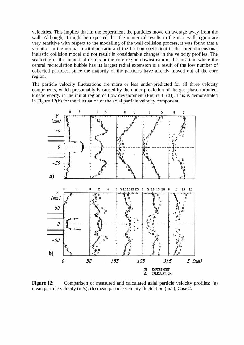
velocities. This implies that in the experiment the particles move on average away from the wall. Although, it might be expected that the numerical results in the near-wall region are very sensitive with respect to the modelling of the wall collision process, it was found that a variation in the normal restitution ratio and the friction coefficient in the three-dimensional inelastic collision model did not result in considerable changes in the velocity profiles. The scattering of the numerical results in the core region downstream of the location, where the central recirculation bubble has its largest radial extension is a result of the low number of collected particles, since the majority of the particles have already moved out of the core region. The particle velocity fluctuations are more or less under-predicted for all three velocity components, which presumably is caused by the under-prediction of the gas-phase turbulent kinetic energy in the initial region of flow development (Figure 11(d)). This is demonstrated in Figure 12(b) for the fluctuation of the axial particle velocity component.

Figure 12: Comparison of measured and calculated axial particle velocity profiles: (a) mean particle velocity (m/s); (b) mean particle velocity fluctuation (m/s), Case 2.

Figure 13: Comparison of measurements and calculations: (a) radial particle velocity (m/s); (b) tangential particle velocity (m/s), Case 2. The calculated particle mass flux shows very good agreement with the experiments in the initial region just downstream of the inlet, namely at z = 52 mm, and further downstream at z = 315 (Figure 14(a)). In the intermediate region, where the particles rebound from the wall and interact again with the central recirculation bubble (see Figure 7), some differences between the experiments and predictions are observed in the near-wall region. At z = 155 and 195 mm, the measurements show a relatively narrow layer of particles near the wall with the maximum being directly at the wall. The calculations show a slightly wider particle layer with a maximum in the particle mass flux located at a radial position of 65 mm, which might result from the assumptions made in the particle-wall collision model. A sensitive study, by using different normal restitution ratios and wall friction coefficients in the particle-wall collision model, shows that their influence on the particle mass flux distribution at z = 155 and 195 mm is not too strong (Figure 15). A reduction in the normal restitution ratio from 0.8 to 0.6 gives a slightly narrower particle layer with a more pronounced maximum closer to the wall. When the particle lift force is switched off in the calculations, the particle layer becomes wider with a less pronounced maximum in the mass flux distribution near the wall. This also shows that the particle lift force due to rotation is only important in the near-wall region, where high rotational velocities are induced by the

wall collision. Since the particles lag behind the air flow in the near-wall region, the direction of the lift force is directed towards the centreline. From these results, one may conclude that the particle motion in the near-wall region might also be affected by electrostatic forces, although the Plexiglas test section was carefully grounded.

Figure 14: Measured and calculated axial particle mass flux at z = 115 and 195 mm for different parameters in the wall collision model: ∆, with lift force, e = 0.8, µ = 0.3; ◊, with lift force, e = 0.6, µ = 0.3; *, without lift force, e = 0.8, µ = 0.3; �, experiment, Case 2. In the publications of Sommerfeld et al. (1992) additional numerical results for the swirl Case 1 may be found. Details on measured and calculated particle size-velocity correlations are presented in Sommerfeld and Qiu (1993).

Figure 15: Measured and calculated axial particle mass flux at z = 115 and 195 mm for different parameters in the wall collision model: ∆, with lift force, e = 0.8, µ = 0.3; ◊, with lift force, e = 0.6, µ = 0.3; *, without lift force, e = 0.8, µ = 0.3; �, experiment, Case 2. The test case particle-laden swirling flow (here Case 1) was used for validation of „in-house“ codes at the 5th Workshop on Two Phase Flow Predictions (Sommerfeld and Wennerberg 1991). Several groups have participated in these calculations and the results may be found in the Workshop Proceedings, including a description of the numerical methods applied. Most of the calculations were performed with the two-dimensional Euler/Lagrange approach (e.g. Azevedo/Pereira, Milojevic, Wennerberg, Berlemont, Blümcke and Ando/Sommerfeld). Regarding the fluid flow mostly the standard k-ε turbulence model was used, some participants adapted however the model constants (i.e. Blümcke). Moreover, some contributions were based on the application of algebraic stress models in order to predict the stress components of the fluid, which were also used for the particle tracking (e.g. Berlemont and Wennerberg). The two-fluid approach was only applied by Simonin also using a k-ε turbulence model. The fluctuating motion of the dispersed phase was linked to the continuous phase turbulence through analytic correlations (Simonin 1991). Some results of the test case calculations for Case 1 are shown below (Fig. 16 to 23), revealing that there is a noticeable scatter of the calculations performed by the different groups. The mean velocities for gas and particle phase are captured reasonably well, but all components of the fluctuating velocities are generally considerably under-predicted, for both gas and particles. In the numerical calculation of the particle mass flux profiles the critical issue is the prediction of the correct penetration of the particles into the central recirculation region. At the end of the recirculation region mostly the particle mass flux is under-predicted. Surprisingly, the profiles of the particle number mean diameter are captured quite well by most of the computations.

Figure 16: Measured and calculated axial gas-phase mean velocity profiles presented at the 5th Workshop on Two-Phase Flow Predictions, Case 1.

Figure 17: Measured and calculated axial gas-phase rms velocity profiles presented at the 5th Workshop on Two-Phase Flow Predictions, Case 1.

Figure 18: Measured and calculated tangential gas-phase mean velocity profiles presented at the 5th Workshop on Two-Phase Flow Predictions, Case 1.

Figure 19: Measured and calculated axial particle mean velocity profiles presented at the 5th Workshop on Two-Phase Flow Predictions, Case 1.

Figure 20: Measured and calculated axial particle mean velocity profiles presented at the 5th Workshop on Two-Phase Flow Predictions, Case 1.

Figure 21: Measured and calculated tangential particle-phase mean velocity profiles presented at the 5th Workshop on Two-Phase Flow Predictions, Case 1.

Figure 22: Measured and calculated particle mass flux in the stream-wise direction presented at the 5th Workshop on Two-Phase Flow Predictions, Case 1.

Figure 23: Measured and calculated particle mean number diameter presented at the 5th Workshop on Two-Phase Flow Predictions, Case 1.

5. BEST PRACTICE ADVICE

5.1 KEY FLUID PHYSICS

The introduced swirling flows are highly turbulent and as known, the turbulence structure is strongly anisotropic. Moreover, the flow is characterized by a central recirculation region and a flow separation in the pipe expansion. Mostly such kind of flows is not stationary, but exhibit some fluctuations of the vortex core (precessing). This effect also influences the particle behaviour which is manifested in the formation of particle ropes. These are caused by slight fluctuations of the particle-laden primary jet induced by the vortex precession. Eventually these ropes move spirally along the test section wall downward. As a consequence of the locally high particle concentration two-way coupling effects and also inter-particle collisions might become of importance.

5.2 APPLICATION UNCERTAINITIES

The flow geometry is relatively simple and can be accurately specified and discretised. The inlet conditions were measured 3 mm downstream the exit of the inlet tubes so that the variation of the flow during the first 3 mm (i.e. from the exact geometrical exit) can be neglected. In previous calculations the particle size at the tube exit was specified according to that provided in Fig. 2. The first measured profile reveals that a spatial variation of the particle size distribution at the exit can be neglected. Possibly however, the mean velocity and the rms values for the different particle size classes might be slightly different. It should be also kept in mind that the measurements were only done for one profile across the test section. Hence any asymmetries of the flow could bias the results.

5.3 COMPUTATIONAL DOMAIN AND BOUNDARY CONDITIONS

Previous calculations have been done based on the two-dimensional axisymmetric conservation equations. As a matter of fact however the flow should be considered as fully three-dimensional and possibly the computations should be done using an unsteady approach in order to capture the slight precessing of the swirling vortex. This will also affect the particle behaviour and it is possible to numerically predict particle rope formation and dispersion (Lipowsky and Sommerfeld 2007, Sommerfeld et al. 2010).

5.4 DISCRETISATION AND GRID RESOLUTION

For full three-dimensional calculations of the considered swirling flow at least 300,000 control volumes should be used when applying RANS methods. In the case of LES the grid resolution should be much higher. Apte et al. (2003) have for example used 1.6 million hexahedral volumes. For steady-state calculations several hundred thousands of particles should be sufficient. For unsteady simulations the number of considered particles needs to be higher in order to ensure good statistical averaging.

5.5 PHYSICAL MODELLING

It is suggested to calculate the swirling flow either with a Reynolds-stress turbulence model or applying LES. Due to the singularity at r = 0 in a cylindrical frame of reference, particle tracking should be done on a Cartesian coordinate system. Since the particles are relatively small transverse lift forces have not a very strong effect on the particle motion and the resulting concentration profiles (see Sommerfeld and Qiu 1993).

5.6 RECOMMENDATIONS FOR FUTURE WORK

The described test cases for particle-laden swirling flows provide very detailed measurements for air- and particle-phase properties. It would be interesting to see a comparison of steady and unsteady calculations as well as calculation results obtained with different turbulence closures, including LES. Moreover, in the case of rope formation (unsteady simulations) the effect of two-way coupling and inter-particle collisions should be evaluated.

REFERENCES

Apte, S.V., Mahesh, K., Moin, P. and Oefelein, J.C.: Large-eddy simulation of swirling particle-laden flows in a coaxial-jet combustor. International Journal of Multiphase Flow, 29 (2003) 1311-1331 Demirdzic, I. and Peric, M.: Finite volume method in arbitrarily shaped domains with moving boundaries. Int. J. for Numerical Methods in Fluids, Vol. 10, 771 – 790 (1990) Lipowsky, J. and Sommerfeld, M.: LES-simulation of the formation of particle strands in swirling flows using an unsteady Euler-Lagrange approach. Proceedings of the 6th International Conference on Multiphase Flow, ICMF2007, Leipzig Germany, Paper No. S3_Thu_C_54 (2007) Peric, M., Kessler, R. and Scheurer, G.: Comparison of finite-volume numerical methods with staggered and co-located grids. Computers and Fluids, Vol. 6, 389 – 403 (1988) Simonin, O.: “Prediction of the dispersed phase turbulence in particle laden jets”, Gas-Solid Flows (Eds. D.E. Stock et al.), ASME-JSME Fluids Engineering Conference, FED-Vol. 121, 197-206 (1991) Sommerfeld, M. and Qiu, H.-H.: Detailed measurements in a swirling particulate two-phase flow by a phase-Doppler anemometer. International Journal of Heat and Fluid Flow, Vol. 12, 20-28 (1991) Sommerfeld, M. and Wennerberg, D. (Eds.): Proceedings 5th Workshop on Two-Phase Flow Predictions, Erlangen 1990, Bilateral Seminars of the International Bureau Forschungszentrum Jülich, (1991) Sommerfeld, M., Ando, A. and Wennerberg, D.: Swirling, particle-laden flows through a pipe expansion. Journal of Fluids Engineering, Vol. 114, 648-656 (1992) Sommerfeld, M. and Qiu, H.-H.: Characterization of particle-laden, confined swirling flows by phase-Doppler anemometry and numerical calculation. Int. Journal Multiphase Flow, Vol. 19, 1093-1127 (1993) Sommerfeld, M., Kohnen, G. and Rüger, M.: Some open questions and inconsistencies of Lagrangian Particle dispersion models. Ninth Symposium on Turbulent Shear Flows, Kyoto, Aug. 1993, Paper 15.1.

Sommerfeld, M. and Tropea, C.: Single-Point Laser Measurement. Chapter 7 in Instrumentation for Fluid-Particle Flow (Ed. S.L. Soo), Noyes Publications, 252-317 (1999) Sommerfeld, M., van Wachem, B. and Oliemans, R.: Best Practice Guidelines for Computational Fluid Dynamics of Dispersed Multiphase Flows. ERCOFTAC (European Research Community on Flow, Turbulence and Combustion, ISBN 978-91-633-3564-8 (2008) Sommerfeld, M., Lipowsky, J. and Laín, S. (keynote lecture): Transient Euler/Lagrange modelling for predicting unsteady rope behaviour in gas-particle flows. Proceedings of FEDSM2010 ASME Joint U.S. - European Fluids Engineering Summer Meeting, August 1 – 5, 2010, Montreal, Canada, Paper No. FEDSM-ICNMM2010-31335.