Applicability of Mean Field Approximation to Numerical Experiments of Thermal Convection During the...
7
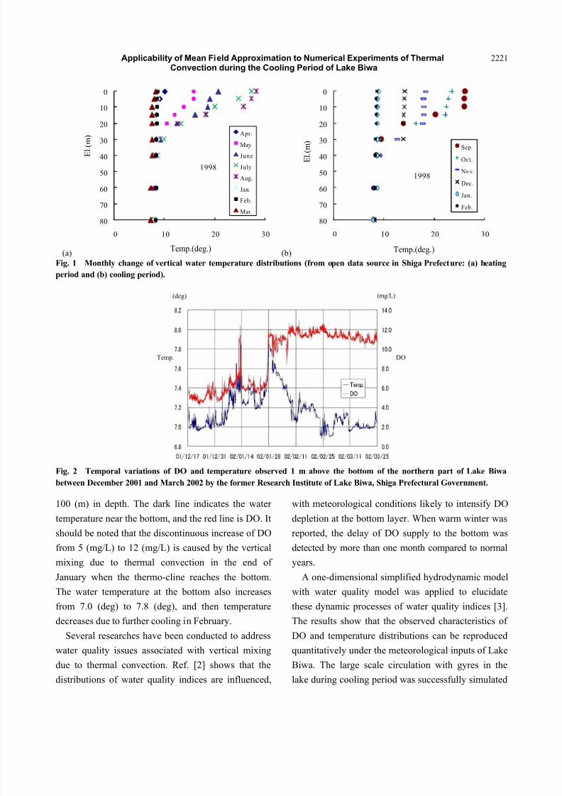
Journal of Energy and Power Engineering 7 (2013) 2220-2226 Applicability of Mean Field Approximation to Numerical Experiments of Thermal Convection during the Cooling Period of Lake Biwa Takashi Hosoda 1 and Frederick Malembeka 2 1. Department of Urban Management, Graduate School of Engineering, Kyoto University, Kyoto 615-8540, Japan 2. Department of Civil Engineering, Arusha Technical College, Arusha 296, Tanzania Received: April 12, 2013 / Accepted: July 16, 2013 / Published: December 31, 2013. Abstract: This paper describes the applicability of a stochastic model to the numerical experiments of thermal convection carried out under the condition of the northern part of Lake Biwa, Shiga Prefecture, Japan. It was shown in the previous study that the temporal changes of vertical water temperature distributions during the cooling period between September and February can be reproduced by a simple 3D-CFD model. It was also pointed out that the spatial distributions of cooled water body sinking to the bottom due to water surface cooling represent similar features of forest gap distribution, which can be clarified by a stochastic model. The basic features of numerical experiments on thermal convection such as the spatial distribution of cooled water body are firstly shown with several cooling rates at water surface. Then, a stochastic model, which was originally introduced to explain forest gap dynamics, is shown with its MFA (mean field approximation) as first approximation of stochastic model. It is pointed out through the comparison of theoretical results by MFA with tuned model constants to numerical experiments that MFA with some refinement can be applicable to reproduce the basic features of simulated results to some extent, although further investigations are required to clarify the applicability of the model to more detailed mechanism of thermal convection such as size distribution of cooled water body, phase change of flow pattern, etc.. Key words: Thermal convection, lake hydrodynamics, Lake Biwa, stochastic model. 1. Introduction Lake Biwa is the largest monomictic lake located in the central part of Japan, having a total surface area of about 670 (km 2 ) and 104 (m) at maximum depth. Its role as the source of water is paramount in supporting the peoples life in nearby prefectures such as Osaka, Kyoto and Shiga. Its value as an ancient lake offering habitat for rare indigenous species warranted it to be vested as UNESCO Ramsar s site. Alarming deterioration of water quality is a main concern with climate change such as increased air temperature being noted to b e linked with cycles of warm winters Corresponding author: Takashi Hosoda, professor, research fields: hydraulic engineering and water environment. E-mail: [email protected]. which are related to low levels of DO (dissolved oxygen) around lakes bottom layer [1]. Fig. 1 shows the monthly changes of water temperature distribution in vertical direction during both the heating period from Ma rch to August and t he cooling period from September to February taken from the open data source of Shiga Prefecture. It can be pointed out that the uniform distributions of temperature near the water surface are clearly observed in the temporal changes from September and February due to thermal convection, and the thermo-cline reaches the bottom in J anuary. Fig. 2 shows the temporal variations of DO observed by the former Lake Biwa Research Instit ute at the bo tt om off th e sh or e of Oh mi- Ima zu wi th ab ou t D DAVID PUBLISHING
-
Upload
energydavid -
Category
Documents
-
view
214 -
download
0
Transcript of Applicability of Mean Field Approximation to Numerical Experiments of Thermal Convection During the...

8/12/2019 Applicability of Mean Field Approximation to Numerical Experiments of Thermal Convection During the Cooling Per…
http://slidepdf.com/reader/full/applicability-of-mean-field-approximation-to-numerical-experiments-of-thermal 1/7
8/12/2019 Applicability of Mean Field Approximation to Numerical Experiments of Thermal Convection During the Cooling Per…
http://slidepdf.com/reader/full/applicability-of-mean-field-approximation-to-numerical-experiments-of-thermal 2/7
Applicability of Mean Field Approximation to Numerical Experiments of ThermalConvection during the Cooling Period of Lake Biwa
2221
(a)
0
10
20
30
40
50
60
70
80
0 10 20 30
E l . ( m )
Temp.(deg.)
1998
Apr.
May
June
July
Aug.
Jan.
Feb.
Mar.
(b)
0
10
20
30
40
50
60
70
80
0 10 20 30
E l . ( m )
Temp.(deg.)
1998
Sep.
Oct.
No v.
Dec.
Jan.
Feb.
Fig. 1 Monthly change of vertical water temperature distributions (from open data source in Shiga Prefecture: (a) heating
period and (b) cooling period).
Fig. 2 Temporal variations of DO and temperature observed 1 m above the bottom of the northern part of Lake Biwa
between December 2001 and March 2002 by the former Research Institute of Lake Biwa, Shiga Prefectural Government.
100 (m) in depth. The dark line indicates the water
temperature near the bottom, and the red line is DO. It
should be noted that the discontinuous increase of DO
from 5 (mg/L) to 12 (mg/L) is caused by the vertical
mixing due to thermal convection in the end of
January when the thermo-cline reaches the bottom.
The water temperature at the bottom also increases
from 7.0 (deg) to 7.8 (deg), and then temperature
decreases due to further cooling in February.
Several researches have been conducted to address
water quality issues associated with vertical mixing
due to thermal convection. Ref. [2] shows that the
distributions of water quality indices are influenced,
with meteorological conditions likely to intensify DO
depletion at the bottom layer. When warm winter was
reported, the delay of DO supply to the bottom was
detected by more than one month compared to normal
years.
A one-dimensional simplified hydrodynamic model
with water quality model was applied to elucidate
these dynamic processes of water quality indices [3].
The results show that the observed characteristics of
DO and temperature distributions can be reproduced
quantitatively under the meteorological inputs of Lake
Biwa. The large scale circulation with gyres in the
lake during cooling period was successfully simulated
(deg) (mg/L)
Temp. DO
8/12/2019 Applicability of Mean Field Approximation to Numerical Experiments of Thermal Convection During the Cooling Per…
http://slidepdf.com/reader/full/applicability-of-mean-field-approximation-to-numerical-experiments-of-thermal 3/7
Applicability of Mean Field Approximation to Numerical Experiments of ThermalConvection during the Cooling Period of Lake Biwa
2222
using a 3-D hydrostatic model [4]. The vertical mixing
mechanism due to thermal convection was also
studied using non-hydrostatic 3-D CFD model
considering the effects of surface processes lumped as
water surface cooling rate [5]. The basic features of
flow patterns induced by thermal convection can be
stated based on simulated results that water bodies
cooled locally at the surface goes down to the bottom
with compensating upward flows around the sinking
water body, inducing the interfacial mixing between
upper and lower layers.
In this paper, a stochastic model which is similar to
forest gap model [6] is applied to explain the basic
features of numerical experiments conducted underthe cooling condition of the lake. The simple
theoretical equation of the ratio of cooled water body
is derived applying the MFA (mean field
approximation) to a stochastic model, and is verified
qualitatively by numerical experiments.
2. Numerical Experiments
2.1 Model Description
Flow mechanism in the lake undergoing thermal
cooling is simulated considering the conservation of
mass, momentum and heat. The basic equations are
described in Eqs. (1)-(5):
0=∂∂
∂∂
∂∂
z
w
y
v
x
u (1)
)
z
(
1
y
2
2
2
2
2
2
∂
∂+
∂
∂+
∂
∂+
∂∂
−=∂∂
+∂∂
+∂∂
+∂∂
u
y
u
x
u
x
p
z
uw
uv
x
uu
t
u
ν
ρ(2)
)z
(
y
1v
2
2
2
2
2
2
∂∂
+∂∂
+∂∂
+
∂∂
−=∂∂
+∂∂
+∂∂
+∂∂
v
y
v
x
v
p
z
vw
y
vv
xu
t
v
ν
ρ (3)
)(
1
2
2
2
2
2
2
z
w
y
w
x
w
z
p g
z
ww
y
wv
x
wu
t
w
∂∂
+∂∂
+∂∂
+
∂∂
−−=∂∂
+∂∂
+∂∂
+∂∂
ν
ρ (4)
∂∂
+∂∂
+∂∂
=∂∂+
∂∂+
∂∂+
∂∂
2
2
2
2
2
2
z
T
y
T
x
T
z
T w
y
T v
x
T u
t
T
(5)
where, ),,( z y x = spatial coordinates, t = time,
),,( wvu = components of velocity vectors, p =
pressure, T = temperature, g = gravity acceleration,
ν = dynamic molecular viscosity, λ = molecular
diffusivity.
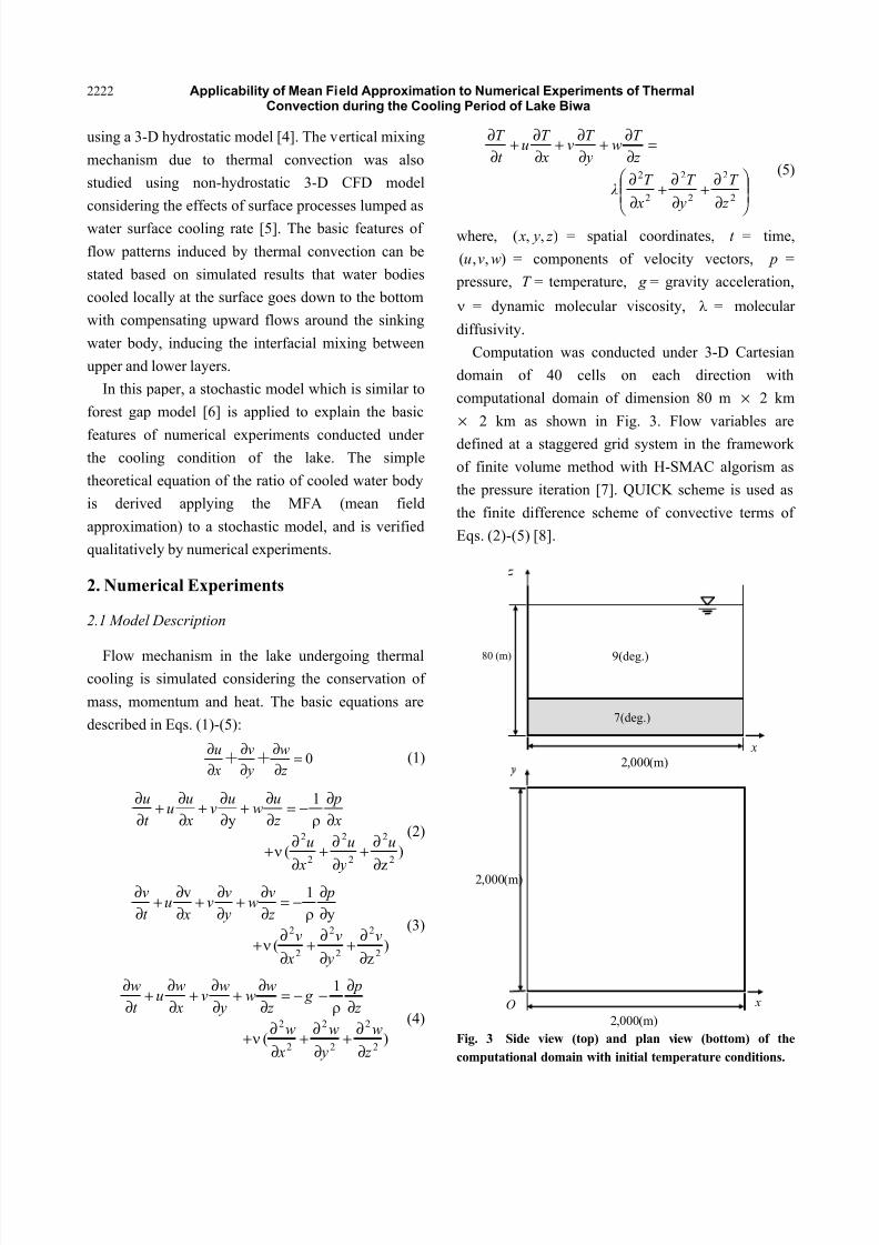
Computation was conducted under 3-D Cartesian
domain of 40 cells on each direction with
computational domain of dimension 80 m × 2 km
× 2 km as shown in Fig. 3. Flow variables are
defined at a staggered grid system in the framework
of finite volume method with H-SMAC algorism as
the pressure iteration [7]. QUICK scheme is used as
the finite difference scheme of convective terms of
Eqs. (2)-(5) [8].
Fig. 3 Side view (top) and plan view (bottom) of the
computational domain with initial temperature conditions.
(m)000,2 x
(deg.)9
(deg.)7
(m)000,2
(m)000,2
O x
80 (m)
8/12/2019 Applicability of Mean Field Approximation to Numerical Experiments of Thermal Convection During the Cooling Per…
http://slidepdf.com/reader/full/applicability-of-mean-field-approximation-to-numerical-experiments-of-thermal 4/7
Applicability of Mean Field Approximation to Numerical Experiments of ThermalConvection during the Cooling Period of Lake Biwa
2223
Considering the thermal condition in January, the
initial water temperature distributions in the vertical
direction are 9 (deg) for 20 (m) < z < 80 (m), and 7
(deg) for z ≤ 20 (m). The cooling process at the
surface is represented as the surface boundary
condition, Eq. (6):
pc
Q
z
T
ρλ 0=
∂∂
(6)
where, 0Q = cooling rate at the surface and pc =
specific heat.
2.2 Results of Numerical Experiments
To understand the basic features of vertical mixing
under different surface cooling processes, severalcooling rates at the surface were tested. For easy
identification, cooling rates are denoted as (Q0)rate,
where the subscript rate indicates a value of surface
cooling rate in cal/cm2/s ! 10
4.
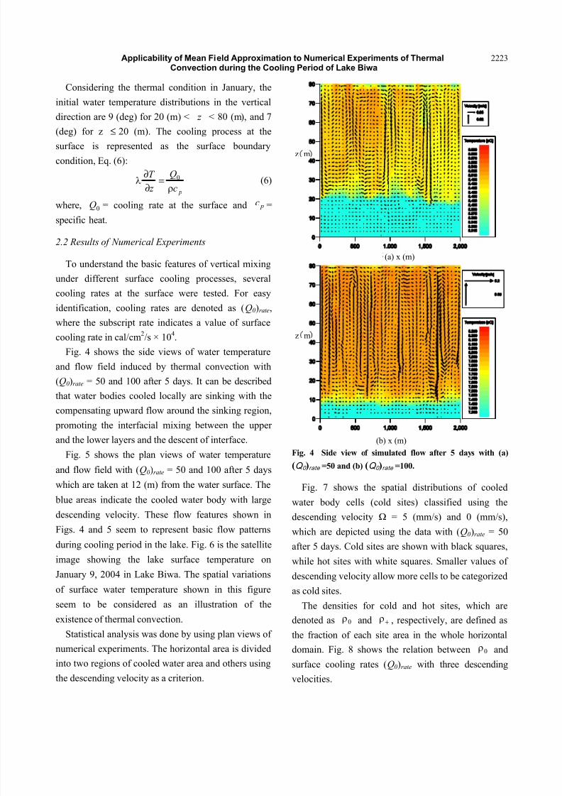
Fig. 4 shows the side views of water temperature
and flow field induced by thermal convection with
(Q0)rate = 50 and 100 after 5 days. It can be described
that water bodies cooled locally are sinking with the
compensating upward flow around the sinking region,
promoting the interfacial mixing between the upper
and the lower layers and the descent of interface.
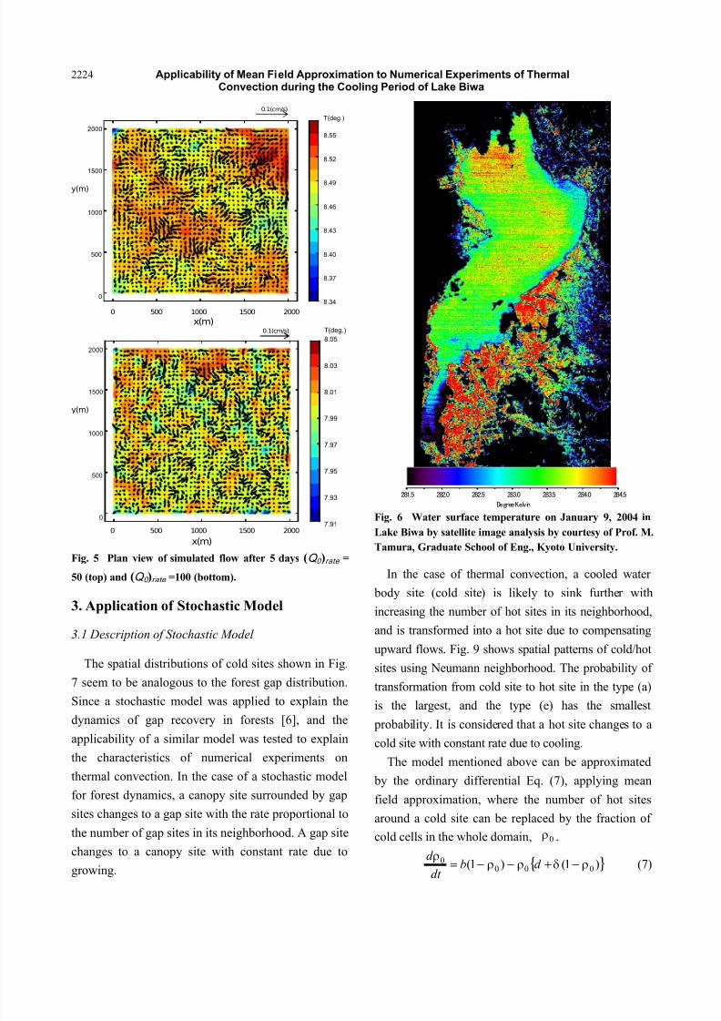
Fig. 5 shows the plan views of water temperature
and flow field with (Q0)rate = 50 and 100 after 5 days
which are taken at 12 (m) from the water surface. The
blue areas indicate the cooled water body with large
descending velocity. These flow features shown in
Figs. 4 and 5 seem to represent basic flow patterns
during cooling period in the lake. Fig. 6 is the satellite
image showing the lake surface temperature on
January 9, 2004 in Lake Biwa. The spatial variations
of surface water temperature shown in this figure
seem to be considered as an illustration of the
existence of thermal convection.
Statistical analysis was done by using plan views of
numerical experiments. The horizontal area is divided
into two regions of cooled water area and others using
the descending velocity as a criterion.
Fig. 4 Side view of simulated flow after 5 days with (a)
(Q 0 )rate =50 and (b) (Q 0 )rate =100.
Fig. 7 shows the spatial distributions of cooled
water body cells (cold sites) classified using the
descending velocity ! = 5 (mm/s) and 0 (mm/s),
which are depicted using the data with (Q0)rate = 50
after 5 days. Cold sites are shown with black squares,
while hot sites with white squares. Smaller values of
descending velocity allow more cells to be categorized
as cold sites.
The densities for cold and hot sites, which are
denoted as 0ρ and +ρ , respectively, are defined as
the fraction of each site area in the whole horizontal
domain. Fig. 8 shows the relation between 0ρ and
surface cooling rates (Q0)rate with three descending
velocities.
(a) x (m)
z m
(b) x (m)
z m
8/12/2019 Applicability of Mean Field Approximation to Numerical Experiments of Thermal Convection During the Cooling Per…
http://slidepdf.com/reader/full/applicability-of-mean-field-approximation-to-numerical-experiments-of-thermal 5/7
Applicability of Mean Field Approximation to Numerical Experiments of ThermalConvection during the Cooling Period of Lake Biwa
2224
Fig. 5 Plan view of simulated flow after 5 days (Q 0 )rate =
50 (top) and (Q 0 )rate =100 (bottom).
3. Application of Stochastic Model
3.1 Description of Stochastic Model
The spatial distributions of cold sites shown in Fig.
7 seem to be analogous to the forest gap distribution.
Since a stochastic model was applied to explain the
dynamics of gap recovery in forests [6], and the
applicability of a similar model was tested to explain
the characteristics of numerical experiments on
thermal convection. In the case of a stochastic model
for forest dynamics, a canopy site surrounded by gap
sites changes to a gap site with the rate proportional to
the number of gap sites in its neighborhood. A gap site
changes to a canopy site with constant rate due to
growing.
Fig. 6 Water surface temperature on January 9, 2004 in
Lake Biwa by satellite image analysis by courtesy of Prof. M.Tamura, Graduate School of Eng., Kyoto University.
In the case of thermal convection, a cooled water
body site (cold site) is likely to sink further with
increasing the number of hot sites in its neighborhood,
and is transformed into a hot site due to compensating
upward flows. Fig. 9 shows spatial patterns of cold/hot
sites using Neumann neighborhood. The probability of
transformation from cold site to hot site in the type (a)
is the largest, and the type (e) has the smallest
probability. It is considered that a hot site changes to a
cold site with constant rate due to cooling.
The model mentioned above can be approximated
by the ordinary differential Eq. (7), applying mean
field approximation, where the number of hot sites
around a cold site can be replaced by the fraction of
cold cells in the whole domain, 0ρ .
)1()1( 0000 ρδρρ
ρ−+−−= d b
dt
d (7)
281.5 282.0 282.5 283.0 283.5 284.0 284.5
Degree Kelvin
0 500 1000 1500 2000
T(deg.)
8.55
8.52
8.49
8.46
8.43
8.40
8.37
8.34
x(m)
2000
1500
1000
500
0
y(m)
0.1(cm/s)
0 500 1000 1500 2000
x(m)
2000
1500
1000
500
0
y(m)
T(deg.)
8.05
8.03
8.01
7.99
7.97
7.95
7.93
7.91
0.1(cm/s)

8/12/2019 Applicability of Mean Field Approximation to Numerical Experiments of Thermal Convection During the Cooling Per…
http://slidepdf.com/reader/full/applicability-of-mean-field-approximation-to-numerical-experiments-of-thermal 6/7
Applicability of Mean Field Approximation to Numerical Experiments of ThermalConvection during the Cooling Period of Lake Biwa
2225
Fig. 7 Spatial distributions of cooled water body cells
(cold site) classified by means of descending velocity (top:
Ω = 5 (mm/s), bottom: Ω = 0 (mm/s)).
Fig. 8 Relation between fraction of cold sites and cooling
rate.
where δ,,d b = model constants. Eq. (7) was used as
the first approximation in the forest gap dynamics [6].
The first term on the right of Eq. (7) represents the
transformation from hot site to cold site due to cooling,
and the second term represents the transformation
from cold site to hot site due to sinking.
Fig. 9 Classification of spatial patterns of cold/hot cells
used for a stochastic model.
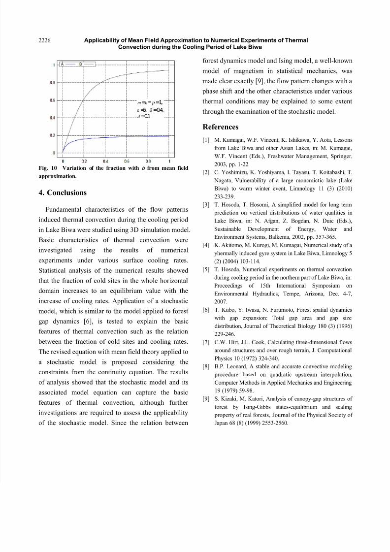
Assuming the steady state by setting the left side to
be zero, 0ρ in the equilibrium state can be evaluated.
0ρ approaches to 1 with increasing cooling rate, b
as shown as Line B in Fig. 10. But, 0ρ in numerical
experiments can not become to 1 as shown in Fig. 8,
because the whole area can not sink due to the
constraints from the continuity Eq. (1).
Considering the constraints of continuity, Eq. (8) is
proposed with the revised form in the second term on
the right of Eq. (8), where the rate of transformation
from cold site to hot site is reduced with increasing
the fraction of cold site.
( ) p
mn d
bdt
d
0
000
0
1
)1()1(
ερ
ρδρρ
ρ
+
−+−−= (8)
Line A in Fig. 10 is evaluated using Eq. (8) with
constants m = n = p =1, ε = 5, δ = 0.4 and d = 0.1.
With increasing the cooling rate, b, 0ρ becomes to a
constant value less than 1. These results indicate that
some basic features of numerical experiments on
thermal convection can be reproduced by using the
simple stochastic model, although more detailed
comparisons between numerical experiments and
theoretical results with various flow conditions are
required to assess the stochastic model.
a
b
Hot Site
Cold
c
d
0ρ
rate )(Q0
8/12/2019 Applicability of Mean Field Approximation to Numerical Experiments of Thermal Convection During the Cooling Per…
http://slidepdf.com/reader/full/applicability-of-mean-field-approximation-to-numerical-experiments-of-thermal 7/7
Applicability of Mean Field Approximation to Numerical Experiments of ThermalConvection during the Cooling Period of Lake Biwa
2226
Fig. 10 Variation of the fraction with b from mean field
approximation.
4. Conclusions
Fundamental characteristics of the flow patterns
induced thermal convection during the cooling period
in Lake Biwa were studied using 3D simulation model.
Basic characteristics of thermal convection were
investigated using the results of numerical
experiments under various surface cooling rates.
Statistical analysis of the numerical results showed
that the fraction of cold sites in the whole horizontal
domain increases to an equilibrium value with the
increase of cooling rates. Application of a stochastic
model, which is similar to the model applied to forest
gap dynamics [6], is tested to explain the basic
features of thermal convection such as the relation
between the fraction of cold sites and cooling rates.
The revised equation with mean field theory applied to
a stochastic model is proposed considering the
constraints from the continuity equation. The results
of analysis showed that the stochastic model and its
associated model equation can capture the basic
features of thermal convection, although further
investigations are required to assess the applicability
of the stochastic model. Since the relation between
forest dynamics model and Ising model, a well-known
model of magnetism in statistical mechanics, was
made clear exactly [9], the flow pattern changes with a
phase shift and the other characteristics under various
thermal conditions may be explained to some extent
through the examination of the stochastic model.
References
[1] M. Kumagai, W.F. Vincent, K. Ishikawa, Y. Aota, Lessons
from Lake Biwa and other Asian Lakes, in: M. Kumagai,
W.F. Vincent (Eds.), Freshwater Management, Springer,
2003, pp. 1-22.
[2] C. Yoshimizu, K. Yoshiyama, I. Tayasu, T. Koitabashi, T.
Nagata, Vulnerability of a large monomictic lake (Lake
Biwa) to warm winter event, Limnology 11 (3) (2010)
233-239.
[3] T. Hosoda, T. Hosomi, A simplified model for long term
prediction on vertical distributions of water qualities in
Lake Biwa, in: N. Afgan, Z. Bogdan, N. Duic (Eds.),
Sustainable Development of Energy, Water and
Environment Systems, Balkema, 2002, pp. 357-365.
[4] K. Akitomo, M. Kurogi, M. Kumagai, Numerical study of a
yhermally induced gyre system in Lake Biwa, Limnology 5
(2) (2004) 103-114.
[5] T. Hosoda, Numerical experiments on thermal convection
during cooling period in the northern part of Lake Biwa, in:
Proceedings of 15th International Symposium on
Environmental Hydraulics, Tempe, Arizona, Dec. 4-7,
2007.
[6] T. Kubo, Y. Iwasa, N. Furumoto, Forest spatial dynamics
with gap expansion: Total gap area and gap size
distribution, Journal of Theoretical Biology 180 (3) (1996)
229-246.
[7] C.W. Hirt, J.L. Cook, Calculating three-dimensional flows
around structures and over rough terrain, J. Computational
Physics 10 (1972) 324-340.
[8] B.P. Leonard, A stable and accurate convective modeling
procedure based on quadratic upstream interpolation,
Computer Methods in Applied Mechanics and Engineering
19 (1979) 59-98.
[9] S. Kizaki, M. Katori, Analysis of canopy-gap structures of
forest by Ising-Gibbs states-equilibrium and scaling
property of real forests, Journal of the Physical Society of
Japan 68 (8) (1999) 2553-2560.
m=n p=1,
ε=5, δ=0.4,d =0.1