
Appendix: Mathematics, Symbols, and Physical...
107
© 2003 by CRC Press LLC APPENDIX Mathematics, Symbols, and Physical Constants Greek Alphabet International System of Units (SI) Definitions of SI Base Units • Names and Symbols for the SI Base Units • SI Derived Units with Special Names and Symbols • Units in Use Together with the SI Conversion Constants and Multipliers Recommended Decimal Multiples and Submultiples • Conversion Factors — Metric to English • Conversion Factors — English to Metric • Conversion Factors — General • T emperature Factors • Conversion of Temperatures Physical Constants General • π Constants • Constants Involving e • Numerical Constants Symbols and Terminology for Physical and Chemical Quantities Elementary Algebra and Geometry Fundamental Properties (Real Numbers) • Exponents • Fractional Exponents • Irrational Exponents • Logarithms • Factorials • Binomial Theorem • Factors and Expansion • Progression • Complex Numbers • Polar Form • Permutations • Combinations • Algebraic Equations • Geometry Determinants, Matrices, and Linear Systems of Equations Determinants • Evaluation by Cofactors • Properties of Determinants • Matrices • Operations • Properties • T ranspose • Identity Matrix • Adjoint • Inverse Matrix • Systems of Linear Equations • Matrix Solution Trigonometry T riangles • T rigonometric Functions of an Angle • Inverse Trigonometric Functions Analytic Geometry Rectangular Coordinates • Distance between Two Points; Slope • Equations of Straight Lines • Distance from a Point to a Line • Circle • Parabola • Ellipse • Hyperbola (e > 1) • Change of Axes Series Bernoulli and Euler Numbers • Series of Functions • Error Function • Series Expansion Differential Calculus Notation • Slope of a Curve • Angle of Intersection of Two Curves • Radius of Curvature • Relative Maxima and Minima • Points of Inflection of a Curve • T aylor’s Formula • Indeterminant Forms • Numerical Methods • Functions of Two Variables • Partial Derivatives Integral Calculus Indefinite Integral • Definite Integral • Properties • Common Applications of the Definite Integral • Cylindrical and Spherical Coordinates • Double Integration • Surface Area and Volume by Double Integration • Centroid Vector Analysis Vectors • Vector Differentiation • Divergence Theorem (Gauss) • Stokes’ Theorem • Planar Motion in Polar Coordinates
Transcript of Appendix: Mathematics, Symbols, and Physical...
© 2003 by CRC Press LLC
A
PPENDIX
Mathematics, Symbols,
and Physical Constants
Greek Alphabet
International System of Units (SI)
D
efinitions of SI Base Units
•
N
ames and Symbols for the SI Base Units
•
SI D
erived Units with Special Names and Symbols
•
U
nits in Use Together with the SI
Conversion Constants and Multipliers
R
ecommended Decimal Multiples and Submultiples
•
Conversion Factors — Metric to English
•
C
onversion Factors — English to Metric
•
C
onversion Factors — General
•
T
emperature Factors
•
C
onversion of Temperatures
Physical Constants
Ge
neral
•
π
C
onstants
•
C
onstants Involving
e
•
N
umerical Constants
Symbols and Terminology for Physical and Chemical Quantities
Elementary Algebra and Geometry
F
undamental Properties (Real Numbers)
•
E
xponents
•
F
ractional Exponents
•
I
rrational Exponents
•
L
ogarithms
•
F
actorials
•
B
inomial Theorem
•
F
actors and Expansion
•
P
rogression
•
C
omplex Numbers
•
P
olar Form
•
P
ermutations
•
C
ombinations
•
Algebraic Equations
•
Ge
ometry
Determinants, Matrices, and Linear Systems of Equations
D
eterminants
•
E
valuation by Cofactors
•
P
roperties of Determinants
•
M
atrices
•
O
perations
•
P
roperties
•
T
ranspose
•
I
dentity Matrix
•
Adjoint
•
I
nverse Matrix
•
S
ystems of Linear Equations
•
M
atrix Solution
Trigonometry
T
riangles
•
T
rigonometric Functions of an Angle
•
I
nverse Trigonometric Functions
Analytic Geometry
R
ectangular Coordinates
•
D
istance between Two Points; Slope
•
E
quations of Straight Lines
•
D
istance from a Point to a Line
•
C
ircle
•
P
arabola
•
El
lipse
•
H
yperbola (
e
> 1)
•
C
hange of Axes
Series
B
ernoulli and Euler Numbers
•
S
eries of Functions
•
Er
ror Function
•
S
eries Expansion
Differential Calculus
N
otation
•
S
lope of a Curve
•
Angle of Intersection of Two Curves
•
R
adius of Curvature
•
R
elative Maxima and Minima
•
P
oints of Inflection of a Curve
•
T
aylor’s Formula
•
I
ndeterminant Forms
• Numerical Methods • Functions of Two Variables • Partial Derivatives
Integral Calculus Indefinite Integral • Definite Integral • Properties • Common Applications of the Definite Integral • Cylindrical and Spherical Coordinates • Double Integration • Surface Area and Volume by Double Integration • Centroid
Vector Analysis Vectors • Vector Differentiation • Divergence Theorem (Gauss) • Stokes’ Theorem • Planar Motion in Polar Coordinates

© 2003 by CRC Press LLC
Special Functions Hyperbolic Functions • Laplace Transforms • z-Transform • Trigonometric Identities • Fourier Series • Functions with Period Other Than 2π • Bessel Functions • Legendre Polynomials •
Laguerre Polynomials • Hermite Polynomials • Orthogonality
Statistics Arithmetic Mean • Median • Mode • Geometric Mean • Harmonic Mean • Variance • Standard Deviation • Coefficient of Variation • Probability • Binomial Distribution • Mean of Binomially Distributed Variable • Normal Distribution • Poisson Distribution
Tables of Probability and Statistics Areas under the Standard Normal Curve • Poisson Distribution • t-Distribution •
χ2 Distribution • Variance Ratio
Tables of Derivatives
Integrals Elementary Forms • Forms Containing (a + bx)
The Fourier Transforms Fourier Transforms • Finite Sine Transforms • Finite Cosine Transforms • Fourier Sine Transforms • Fourier Cosine Transforms • Fourier Transforms
Numerical Methods Solution of Equations by Iteration • Finite Differences • Interpolation
Probability Definitions • Definition of Probability • Marginal and Conditional Probability • Probability Theorems • Random Variable • Probability Function (Discrete Case) • Cumulative Distribution Function (Discrete Case) • Probability Density (Continuous Case) • Cumulative Distribution Function (Continuous Case) • Mathematical Expectation
Positional Notation Change of Base • Examples
Credits
Associations and Societies
Ethics
Greek Alphabet
Greek Letter
Greek Name English Equivalent
Greek Letter
Greek Name
English Equivalent
Α α Alpha a Ν ν Nu nΒ β Beta b Ξ ξ Xi xΓ γ Gamma g Ο ο Omicron o∆ δ Delta d Π π Pi pΕ ε Epsilon e P ρ Rho rΖ ζ Zeta z Σ σ s Sigma sΗ η Eta Τ τ Tau tΘ θ ϑ Theta th Y υ Upsilon uΙ ι Iota i Φ φ ϕ Phi phΚ κ Kappa k X χ Chi chΛ λ Lambda l Ψ ψ Psi psΜ µ Mu m Ω ω Omega o–
e
© 2003 by CRC Press LLC
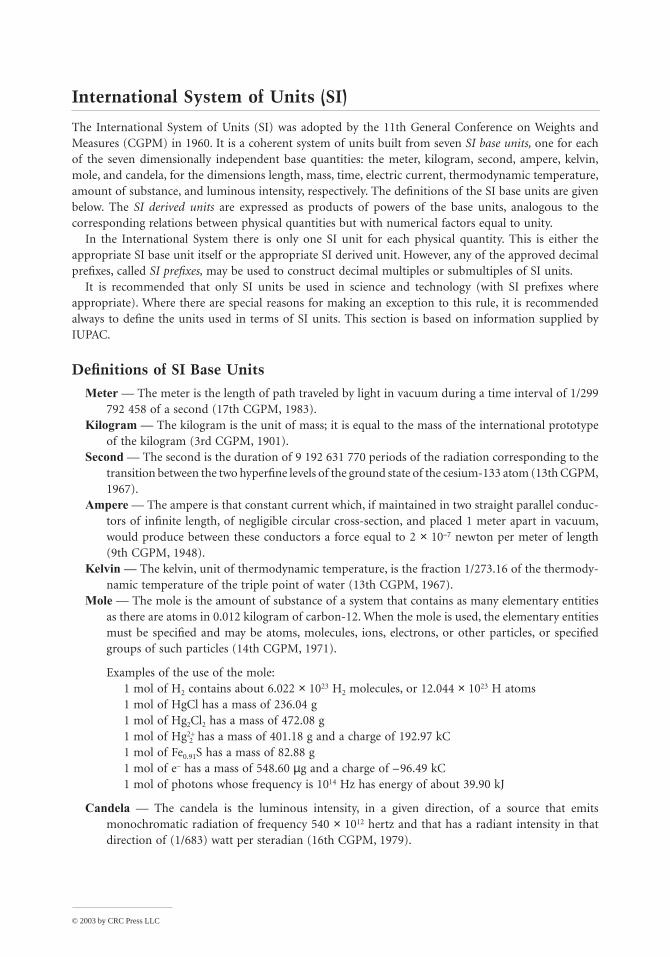
International System of Units (SI)
The International System of Units (SI) was adopted by the 11th General Conference on Weights and Measures (CGPM) in 1960. It is a coherent system of units built from seven SI base units, one for each of the seven dimensionally independent base quantities: the meter, kilogram, second, ampere, kelvin, mole, and candela, for the dimensions length, mass, time, electric current, thermodynamic temperature, amount of substance, and luminous intensity, respectively. The definitions of the SI base units are given below. The SI derived units are expressed as products of powers of the base units, analogous to the corresponding relations between physical quantities but with numerical factors equal to unity.
In the International System there is only one SI unit for each physical quantity. This is either the appropriate SI base unit itself or the appropriate SI derived unit. However, any of the approved decimal prefixes, called SI prefixes, may be used to construct decimal multiples or submultiples of SI units.
It is recommended that only SI units be used in science and technology (with SI prefixes where appropriate). Where there are special reasons for making an exception to this rule, it is recommended always to define the units used in terms of SI units. This section is based on information supplied by IUPAC.
Definitions of SI Base Units
Meter — The meter is the length of path traveled by light in vacuum during a time interval of 1/299 792 458 of a second (17th CGPM, 1983).
Kilogram — The kilogram is the unit of mass; it is equal to the mass of the international prototype of the kilogram (3rd CGPM, 1901).
Second — The second is the duration of 9 192 631 770 periods of the radiation corresponding to the transition between the two hyperfine levels of the ground state of the cesium-133 atom (13th CGPM, 1967).
Ampere — The ampere is that constant current which, if maintained in two straight parallel conduc-tors of infinite length, of negligible circular cross-section, and placed 1 meter apart in vacuum, would produce between these conductors a force equal to 2 × 10⁻⁷ newton per meter of length (9th CGPM, 1948).
Kelvin — The kelvin, unit of thermodynamic temperature, is the fraction 1/273.16 of the thermody-namic temperature of the triple point of water (13th CGPM, 1967).
Mole — The mole is the amount of substance of a system that contains as many elementary entities as there are atoms in 0.012 kilogram of carbon-12. When the mole is used, the elementary entities must be specified and may be atoms, molecules, ions, electrons, or other particles, or specified groups of such particles (14th CGPM, 1971).
Examples of the use of the mole:1 mol of H2 contains about 6.022 × 10²³ H2 molecules, or 12.044 × 10²³ H atoms1 mol of HgCl has a mass of 236.04 g1 mol of Hg2Cl2 has a mass of 472.08 g1 mol of Hg2+
2 has a mass of 401.18 g and a charge of 192.97 kC1 mol of Fe0.91S has a mass of 82.88 g1 mol of e– has a mass of 548.60 µg and a charge of – 96.49 kC1 mol of photons whose frequency is 1014 Hz has energy of about 39.90 kJ
Candela — The candela is the luminous intensity, in a given direction, of a source that emits monochromatic radiation of frequency 540 × 1012 hertz and that has a radiant intensity in that direction of (1/683) watt per steradian (16th CGPM, 1979).
© 2003 by CRC Press LLC
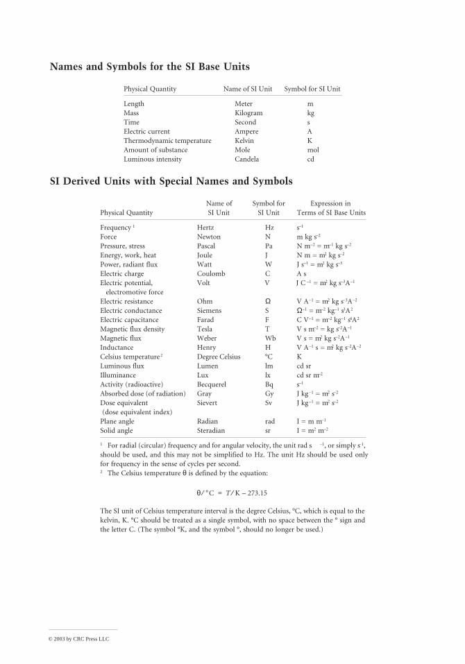
Names and Symbols for the SI Base Units
SI Derived Units with Special Names and Symbols
Physical Quantity Name of SI Unit Symbol for SI Unit
Length Meter mMass Kilogram kgTime Second sElectric current Ampere AThermodynamic temperature Kelvin KAmount of substance Mole molLuminous intensity Candela cd
Physical QuantityName ofSI Unit
Symbol forSI Unit
Expression inTerms of SI Base Units
Frequency 1 Hertz Hz s–1
Force Newton N m kg s–2
Pressure, stress Pascal Pa N m–2 = m–1 kg s–2
Energy, work, heat Joule J N m = m2 kg s–2
Power, radiant flux Watt W J s–1 = m2 kg s–3
Electric charge Coulomb C A sElectric potential,
electromotive forceVolt V J C –1 = m2 kg s–3A–1
Electric resistance Ohm Ω V A–1 = m2 kg s–3A–2
Electric conductance Siemens S Ω–1 = m–2 kg–1 s3A2
Electric capacitance Farad F C V–1 = m–2 kg–1 s4A2
Magnetic flux density Tesla T V s m–2 = kg s–2A–1
Magnetic flux Weber Wb V s = m2 kg s–2A–1
Inductance Henry H V A–1 s = m2 kg s–2A–2
Celsius temperature2 Degree Celsius °C KLuminous flux Lumen lm cd srIlluminance Lux lx cd sr m–2
Activity (radioactive) Becquerel Bq s–1
Absorbed dose (of radiation) Gray Gy J kg –1 = m2 s–2 Dose equivalent (dose equivalent index)
Sievert Sv J kg –1 = m2 s–2
Plane angle Radian rad I = m m–1
Solid angle Steradian sr I = m2 m–2
1 For radial (circular) frequency and for angular velocity, the unit rad s –1, or simply s–1, should be used, and this may not be simplified to Hz. The unit Hz should be used only for frequency in the sense of cycles per second.2 The Celsius temperature θ is defined by the equation:
The SI unit of Celsius temperature interval is the degree Celsius, °C, which is equal to the kelvin, K. °C should be treated as a single symbol, with no space between the ° sign and the letter C. (The symbol °K, and the symbol °, should no longer be used.)
θ °C⁄ T K 273.15–⁄=

© 2003 by CRC Press LLC
Units in Use Together with the SI
These units are not part of the SI, but it is recognized that they will continue to be used in appropriate contexts. SI prefixes may be attached to some of these units, such as milliliter, ml; millibar, mbar; megaelectronvolt, MeV; and kilotonne, ktonne.
Conversion Constants and Multipliers
Recommended Decimal Multiples and Submultiples
Physical Quantity Name of Unit Symbol for Unit Value in SI Units
Time Minute min 60 sTime Hour h 3600 sTime Day d 86 400 sPlane angle Degree ° (π /180) radPlane angle Minute ′ (π /10 800) radPlane angle Second ″ (π /648 000) radLength Ångstrom1 Å 10–10 mArea Barn b 10–28 m2
Volume Liter l, L dm3 = 10–3 m3
Mass Tonne t Mg = 103 kgPressure Bar 1 bar 105 Pa = 105 N m–2
Energy Electronvolt 2 eV (= e × V) ≈ 1.60218 × 10⁻¹⁹ JMass Unified atomic
mass unit2,3
u (= ma(12C)/12) ≈ 1.66054 × 10⁻²⁷ kg
1 The ångstrom and the bar are approved by CIPM for “temporary use with SI units,” until CIPM makes a further recommendation. However, they should not be introduced where they are not used at present.2 The values of these units in terms of the corresponding SI units are not exact, since they depend on the values of the physical constants e (for the electronvolt) and NA (for the unified atomic mass unit), which are deter-mined by experiment.3 The unified atomic mass unit is also sometimes called the dalton, with symbol Da, although the name and symbol have not been approved by CGPM.
Multiples and Submultiples Prefixes Symbols
Multiples and Submultiples Prefixes Symbols
1018 exa E 10–1 deci d1015 peta P 10–2 centi c1012 tera T 10–3 milli m109 giga G 10–6 micro µ (Greek mu)106 mega M 10–9 nano n103 kilo k 10–12 pico p102 hecto h 10–15 femto f10 deca da 10–18 atto a
© 2003 by CRC Press LLC
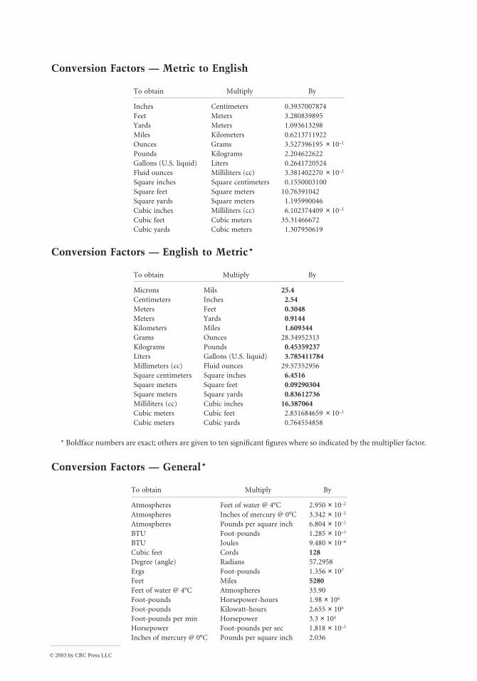
Conversion Factors — Metric to English
Conversion Factors — English to Metric*
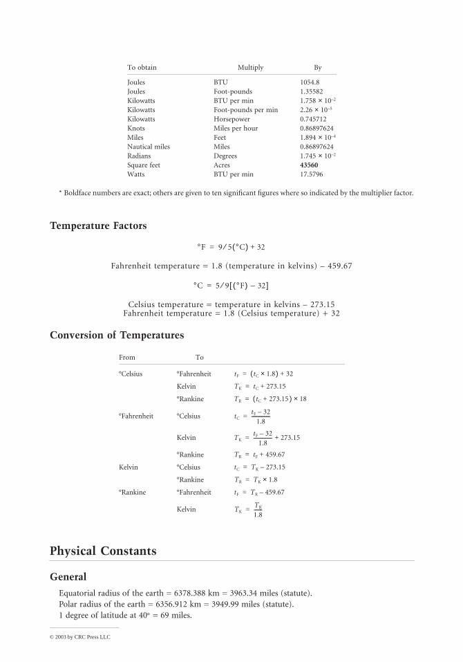
* Boldface numbers are exact; others are given to ten significant figures where so indicated by the multiplier factor.
Conversion Factors — General*
To obtain Multiply By
Inches Centimeters 0.3937007874Feet Meters 3.280839895Yards Meters 1.093613298Miles Kilometers 0.6213711922Ounces Grams 3.527396195 × 10⁻²
Pounds Kilograms 2.204622622Gallons (U.S. liquid) Liters 0.2641720524Fluid ounces Milliliters (cc) 3.381402270 × 10⁻²
Square inches Square centimeters 0.1550003100Square feet Square meters 10.76391042Square yards Square meters 1.195990046Cubic inches Milliliters (cc) 6.102374409 × 10⁻²
Cubic feet Cubic meters 35.31466672Cubic yards Cubic meters 1.307950619
To obtain Multiply By
Microns Mils 25.4Centimeters Inches 2.54Meters Feet 0.3048Meters Yards 0.9144Kilometers Miles 1.609344Grams Ounces 28.34952313Kilograms Pounds 0.45359237Liters Gallons (U.S. liquid) 3.785411784Millimeters (cc) Fluid ounces 29.57352956Square centimeters Square inches 6.4516Square meters Square feet 0.09290304Square meters Square yards 0.83612736Milliliters (cc) Cubic inches 16.387064Cubic meters Cubic feet 2.831684659 × 10⁻²
Cubic meters Cubic yards 0.764554858
To obtain Multiply By
Atmospheres Feet of water @ 4°C 2.950 × 10⁻²
Atmospheres Inches of mercury @ 0°C 3.342 × 10⁻²
Atmospheres Pounds per square inch 6.804 × 10⁻²
BTU Foot-pounds 1.285 × 10⁻³
BTU Joules 9.480 × 10⁻⁴
Cubic feet Cords 128Degree (angle) Radians 57.2958Ergs Foot-pounds 1.356 × 10⁷
Feet Miles 5280Feet of water @ 4°C Atmospheres 33.90Foot-pounds Horsepower-hours 1.98 × 10⁶
Foot-pounds Kilowatt-hours 2.655 × 10⁶
Foot-pounds per min Horsepower 3.3 × 10⁴
Horsepower Foot-pounds per sec 1.818 × 10⁻³
Inches of mercury @ 0°C Pounds per square inch 2.036
© 2003 by CRC Press LLC
* Boldface numbers are exact; others are given to ten significant figures where so indicated by the multiplier factor.
Temperature Factors
Fahrenheit temperature = 1.8 (temperature in kelvins) – 459.67
Celsius temperature = temperature in kelvins – 273.15Fahrenheit temperature = 1.8 (Celsius temperature) + 32
Conversion of Temperatures
Physical Constants
General
Equatorial radius of the earth = 6378.388 km = 3963.34 miles (statute).Polar radius of the earth = 6356.912 km = 3949.99 miles (statute).1 degree of latitude at 40° = 69 miles.
Joules BTU 1054.8Joules Foot-pounds 1.35582Kilowatts BTU per min 1.758 × 10⁻²
Kilowatts Foot-pounds per min 2.26 × 10⁻⁵
Kilowatts Horsepower 0.745712Knots Miles per hour 0.86897624Miles Feet 1.894 × 10⁻⁴
Nautical miles Miles 0.86897624Radians Degrees 1.745 × 10⁻²
Square feet Acres 43560Watts BTU per min 17.5796
From To
°Celsius °Fahrenheit
Kelvin
°Rankine
°Fahrenheit °Celsius
Kelvin
°Rankine
Kelvin °Celsius
°Rankine
°Rankine °Fahrenheit
Kelvin
To obtain Multiply By
°F 9 5 °C( )⁄ 32+=
°C 5 9 °F( ) 32–[ ]⁄=
tF tC 1.8×( ) 32+=
TK tC 273.15+=
TR tC 273.15+( ) 18×=
tCtF 32–
1.8---------------=
TKtF 32–
1.8--------------- 273.15+=
TR tF 459.67+=
tC TK 273.15–=
TR TK 1.8×=
tF TR 459.67–=
TKTR
1.8-------=
© 2003 by CRC Press LLC
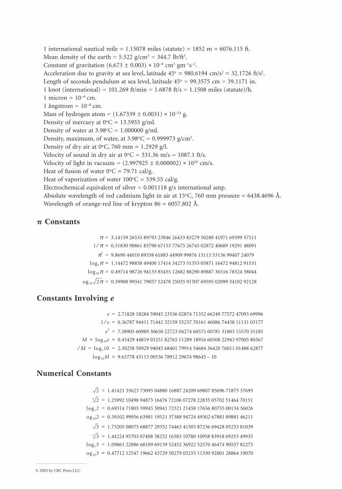
1 international nautical mile = 1.15078 miles (statute) = 1852 m = 6076.115 ft.Mean density of the earth = 5.522 g/cm3 = 344.7 lb/ft3.Constant of gravitation (6.673 ± 0.003) × 10–8 cm3 gm–1s–2.Acceleration due to gravity at sea level, latitude 45° = 980.6194 cm/s2 = 32.1726 ft/s2.Length of seconds pendulum at sea level, latitude 45° = 99.3575 cm = 39.1171 in.1 knot (international) = 101.269 ft/min = 1.6878 ft/s = 1.1508 miles (statute)/h.1 micron = 10–4 cm.1 ångstrom = 10–8 cm.Mass of hydrogen atom = (1.67339 ± 0.0031) × 10–24 g.Density of mercury at 0°C = 13.5955 g/ml.Density of water at 3.98°C = 1.000000 g/ml.Density, maximum, of water, at 3.98°C = 0.999973 g/cm3.Density of dry air at 0°C, 760 mm = 1.2929 g/l.Velocity of sound in dry air at 0°C = 331.36 m/s = 1087.1 ft/s.Velocity of light in vacuum = (2.997925 ± 0.000002) × 1010 cm/s.Heat of fusion of water 0°C = 79.71 cal/g.Heat of vaporization of water 100°C = 539.55 cal/g.Electrochemical equivalent of silver = 0.001118 g/s international amp.Absolute wavelength of red cadmium light in air at 15°C, 760 mm pressure = 6438.4696 Å.Wavelength of orange-red line of krypton 86 = 6057.802 Å.
Constants
Constants Involving e
Numerical Constants
π 3.14159 26535 89793 23846 26433 83279 50288 41971 69399 37511=
1 π⁄ 0.31830 98861 83790 67153 77675 26745 02872 40689 19291 48091=
π2 9.8690 44010 89358 61883 44909 99876 15113 53136 99407 24079=
log eπ 1.14472 98858 49400 17414 34273 51353 05871 16472 94812 91531=
log 10π 0.49714 98726 94133 85435 12682 88290 89887 36516 78324 38044=
og 10 2π 0.39908 99341 79057 52478 25035 91507 69595 02099 34102 92128=
e 2.71828 18284 59045 23536 02874 71352 66249 77572 47093 69996=
1 e⁄ 0.36787 94411 71442 32159 55237 70161 46086 74458 11131 03177=
e2 7.38905 60989 30650 22723 04274 60575 00781 31803 15570 55185=
M log 10e 0.43429 44819 03251 82765 11289 18916 60508 22943 97005 80367= =
1 M⁄ log e10 2.30258 50929 94045 68401 79914 54684 36420 76011 01488 62877= =
log 10M 9.63778 43113 00536 78912 29674 98645 – 10=
2 1.41421 35623 73095 04880 16887 24209 69807 85696 71875 37695=
23 1.25992 10498 94873 16476 72106 07278 22835 05702 51464 70151=
log e2 0.69314 71805 59945 30941 72321 21458 17656 80755 00134 36026=
og 102 0.30102 99956 63981 19521 37388 94724 49302 67881 89881 46211=
3 1.73205 08075 68877 29352 74463 41505 87236 69428 05253 81039=
33 1.44224 95703 07408 38232 16383 10780 10958 83918 69253 49935=
log e3 1.09861 22886 68109 69139 52452 36922 52570 46474 90557 82275=
og 103 0.47712 12547 19662 43729 50279 03255 11530 92001 28864 19070=
© 2003 by CRC Press LLC
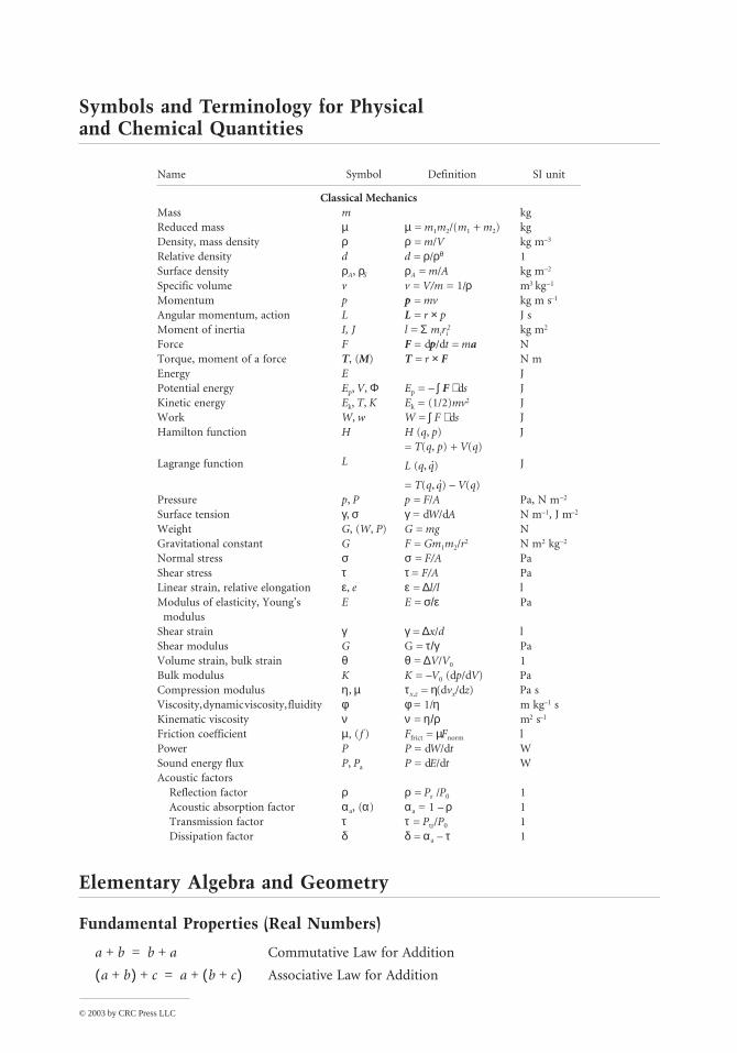
Symbols and Terminology for Physical and Chemical Quantities
Elementary Algebra and Geometry
Fundamental Properties (Real Numbers)
Commutative Law for Addition
Associative Law for Addition
Name Symbol Definition SI unit
Classical MechanicsMass m kgReduced mass µ µ = m1m2/(m1 + m2) kgDensity, mass density ρ ρ = m/V kg m–3
Relative density d d = ρ/ρθ 1Surface density ρA, ρS ρA = m/A kg m–2
Specific volume v v = V/m = 1/ρ m3 kg–1
Momentum p p = mv kg m s–1
Angular momentum, action L L = r × p J sMoment of inertia I, J l = Σ miri
2 kg m2
Force F F = dp/dt = ma NTorque, moment of a force T, (M) T = r × F N mEnergy E JPotential energy Ep, V, Φ Ep = – ∫ F ⋅ ds JKinetic energy Ek, T, K Ek = (1/2)mv2 JWork W, w W = ∫ F ⋅ ds JHamilton function H H (q, p) J
= T(q, p) + V(q)
Lagrange function L L (q, ·q) J
= T(q, ·q) – V(q)Pressure p, P p = F/A Pa, N m–2
Surface tension γ, σ γ = dW/dA N m–1, J m–2
Weight G, (W, P) G = mg NGravitational constant G F = Gm1m2/r2 N m2 kg–2
Normal stress σ σ = F/A PaShear stress τ τ = F/A PaLinear strain, relative elongation ε, e ε = ∆l/l lModulus of elasticity, Young’s
modulusE E = σ/ε Pa
Shear strain γ γ = ∆x/d lShear modulus G G = τ/γ PaVolume strain, bulk strain θ θ = ∆V/V0 1Bulk modulus K K = –V0 (dp/dV) PaCompression modulus η, µ τx,z = η(dvx/dz) Pa sViscosity, dynamic viscosity, fluidity φ φ = 1/η m kg–1 sKinematic viscosity ν ν = η/ρ m2 s–1
Friction coefficient µ, ( f ) Ffrict = µFnorm lPower P P = dW/dt WSound energy flux P, Pa P = dE/dt WAcoustic factors
Reflection factor ρ ρ = Pr /P0 1 Acoustic absorption factor αa, (α) αa = 1 – ρ 1 Transmission factor τ τ = Ptr/P0 1 Dissipation factor δ δ = αa – τ 1
a b+ b a+=
a b+( ) c+ a b c+( )+=
© 2003 by CRC Press LLC
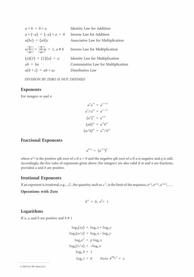
Identity Law for Addition
Inverse Law for Addition
Associative Law for Multiplication
Inverse Law for Multiplication
Identity Law for Multiplication
Commutative Law for Multiplication
Distributive Law
DIVISION BY ZERO IS NOT DEFINED
Exponents
For integers m and n
Fractional Exponents
where a1/q is the positive qth root of a if a > 0 and the negative qth root of a if a is negative and q is odd. Accordingly, the five rules of exponents given above (for integers) are also valid if m and n are fractions, provided a and b are positive.
Irrational Exponents
If an exponent is irrational, e.g., , the quantity, such as , is the limit of the sequence, a1.4, a1.41, a1.414, K .
Operations with Zero
Logarithms
If x, y, and b are positive and b ≠ 1
a 0+ 0 a+=
a a–( )+ a–( ) a+ 0= =
a bc( ) ab( )c=
a 1a--
1a--
a 1 a 0≠,= =
a( ) 1( ) 1( ) a( ) a= =
ab ba=
a b c+( ) ab ac+=
anam an m+=
an am⁄ an m–=
an( )manm=
ab( )m ambm=
a b⁄( )m am bm⁄=
ap q⁄ a1 q⁄( )p=
2 a 2
0m 0 a0; 1= =
logb xy( ) logb x logb y+=
logb x y⁄( ) logb x logb y–=
logbx p p logb x=
logb 1 x⁄( ) logb x–=
logb b 1=
logb 1 0 Note: b bxlog
x= =
© 2003 by CRC Press LLC
Change of Base (a ≠ 1)
Factorials
The factorial of a positive integer n is the product of all the positive integers less than or equal to the integer n and is denoted n!. Thus,
Factorial 0 is defined: 0! = 1.
Stirling’s Approximation
Binomial Theorem
For positive integer n
Factors and Expansion
Progression
An arithmetic progression is a sequence in which the difference between any term and the preceding term is a constant (d ):
If the last term is denoted l [= a + (n – 1) d ], then the sum is
A geometric progression is a sequence in which the ratio of any term to the preceding term is a constant r. Thus, for n terms
logb x loga x logb a=
n! 1 2 3 … n⋅ ⋅ ⋅ ⋅=
n e⁄( )n 2πnn ∞→lim n!=
x y+( )n xn nxn 1– y n n 1–( )2!
--------------------xn 2– y2 n n 1–( ) n 2–( )3!
-------------------------------------xn 3– y3L nxyn 1– yn+ + + + + +=
a b+( )2 a2 2ab b2+ +=
a b–( )2 a2 2ab– b2+=
a b+( )3 a3 3a2b 3ab2 b3+ + +=
a b–( )3 a3 3a2b– 3ab2 b3–+=
a2 b2–( ) a b–( ) a b+( )=
a3 b3–( ) a b–( ) a2 ab b2+ +( )=
a3 b3+( ) a b+( ) a2 ab– b2+( )=
a a d a 2d K a n 1–( )d+, ,+,+,
s n2--- a l+( )=
a ar ar2K arn 1–, ,,,
© 2003 by CRC Press LLC
the sum is
Complex Numbers
A complex number is an ordered pair of real numbers (a, b).
Equality: (a, b) = (c, d ) if and only if a = c and b = dAddition: (a, b) + (c, d ) = (a + c, b + d )Multiplication: (a, b)(c, d ) = (ac – bd, ad + bc)
The first element (a, b) is called the real part; the second is the imaginary part. An alternate notation for (a, b) is a + bi, where i2 = (–1, 0), and i = (0, 1) or 0 + 1i is written for this complex number as a convenience. With this understanding, i behaves as a number, i.e., (2 – 3i)(4 + i) = 8 – 12i + 2i – 3i2 = 11 – 10i. The conjugate of a + bi is a – bi and the product of a complex number and its conjugate is a2 + b2. Thus, quotients are computed by multiplying numerator and denominator by the conjugate of the denominator, as illustrated below:
Polar Form
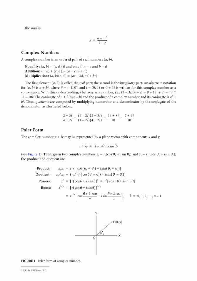
The complex number x + iy may be represented by a plane vector with components x and y
(see Figure 1). Then, given two complex numbers z1 = r1(cos θ1 + i sin θ1) and z2 = r2 (cos θ2 + i sin θ2), the product and quotient are
FIGURE 1 Polar form of complex number.
Sa arn–1 r–
----------------=
2 3i+4 2i+--------------
4 2i–( ) 2 3i+( )4 2i–( ) 4 2i+( )
--------------------------------------14 8i+
20-----------------
7 4i+10
--------------= = =
x iy+ r θ i θsin+cos( )=
Product: z1z2 r1r2 θ1 θ2+( ) i θ1 θ2+( )sin+cos[ ]=
Quotient: z1 z2⁄ r1 r2⁄( ) θ1 θ2–( ) i θ1 θ2–( )sin+cos[ ]=
Powers: zn r θ i θsin+cos( )[ ]n rn nθ i nθsin+cos[ ]= =
Roots: z1 n⁄ r θ i θsin+cos( )[ ] 1 n⁄=
r1 n⁄ θ k.360+n
---------------------- iθ k.360+
n----------------------sin+cos , k 0 1 2 K n, 1–, , ,= =
Y
X0
rP(x, y)
q
© 2003 by CRC Press LLC
Permutations
A permutation is an ordered arrangement (sequence) of all or part of a set of objects. The number of permutations of n objects taken r at a time is
A permutation of positive integers is “even” or “odd” if the total number of inversions is an even integer or an odd integer, respectively. Inversions are counted relative to each integer j in the permutation by counting the number of integers that follow j and are less than j. These are summed to give the total number of inversions. For example, the permutation 4132 has four inversions: three relative to 4 and one relative to 3. This permutation is therefore even.
Combinations
A combination is a selection of one or more objects from among a set of objects regardless of order. The number of combinations of n different objects taken r at a time is
Algebraic Equations
Quadratic
If ax 2 + bx + c = 0, and a ≠ 0, then roots are
Cubic
To solve x 3 + bx 2 + cx + d = 0, let x = y – b/3. Then the reduced cubic is obtained:
where p = c – (1/3)b2 and q = d – (1/3)bc + (2/27)b3. Solutions of the original cubic are then in terms of the reduced cubic roots y1, y2, y3:
The three roots of the reduced cubic are
where
p n r,( ) n n 1–( ) n 2–( )… n r– 1+( )=
n!
n r–( )!------------------=
C n r,( ) P n r,( )r!
----------------n!
r! n r–( )!----------------------= =
xb– b2 4ac–±
2a-------------------------------------=
y3 py q+ + 0=
x1 y1 1 3⁄( )b x2– y2 1 3⁄( )b x3– y3 1 3⁄( )b–= = =
y1 A( )1 3⁄ B( )1 3⁄+=
y2 W A( )1 3⁄ W2 B( )1 3⁄+=
y3 W2 A( )1 3⁄ W B( )1 3⁄+=
A 12--q– 1 27⁄( )p3 1
4--q2++=
© 2003 by CRC Press LLC
When (1/27)p3 + (1/4)q2 is negative, A is complex; in this case A should be expressed in trigono-metric form: A = r (cos θ + i sin θ), where θ is a first- or second-quadrant angle, as q is negative or positive. The three roots of the reduced cubic are
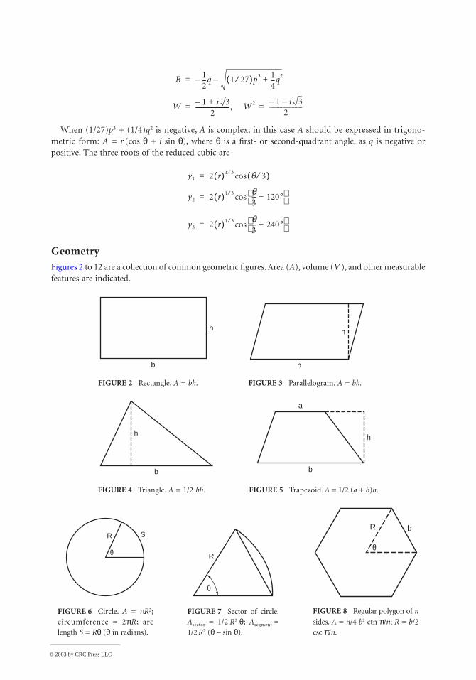
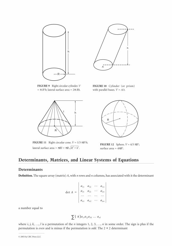
GeometryFigures 2 to 12 are a collection of common geometric figures. Area (A), volume (V ), and other measurable features are indicated.
FIGURE 2 Rectangle. A = bh. FIGURE 3 Parallelogram. A = bh.
FIGURE 4 Triangle. A = 1/2 bh. FIGURE 5 Trapezoid. A = 1/2 (a + b)h.
FIGURE 6 Circle. A = πR2; circumference = 2πR; arc length S = Rθ (θ in radians).
FIGURE 7 Sector of circle. Asector = 1/2 R2 θ; Asegment = 1/2 R2 (θ – sin θ).
FIGURE 8 Regular polygon of n
sides. A = n/4 b2 ctn π/n; R = b/2 csc π/n.
B 12--q– 1 27⁄( )p3 1
4--q2+–=
W 1– i 3+2
----------------------- W 2, 1– i 3–2
----------------------= =
y1 2 r( )1 3⁄ θ 3⁄( )cos=
y2 2 r( )1 3⁄ θ3--- 120°+
cos=
y3 2 r( )1 3⁄ θ3--- 240°+
cos=
b
h h
b
h
b
h
b
a
R S
θ R
θ
θ
R b
© 2003 by CRC Press LLC
Determinants, Matrices, and Linear Systems of Equations
Determinants
Definition. The square array (matrix) A, with n rows and n columns, has associated with it the determinant
a number equal to
where i, j, k, K, l is a permutation of the n integers 1, 2, 3, K, n in some order. The sign is plus if the permutation is even and is minus if the permutation is odd. The 2 × 2 determinant
FIGURE 9 Right circular cylinder. V
= π R2h; lateral surface area = 2π Rh. FIGURE 10 Cylinder (or prism) with parallel bases. V = A/t.
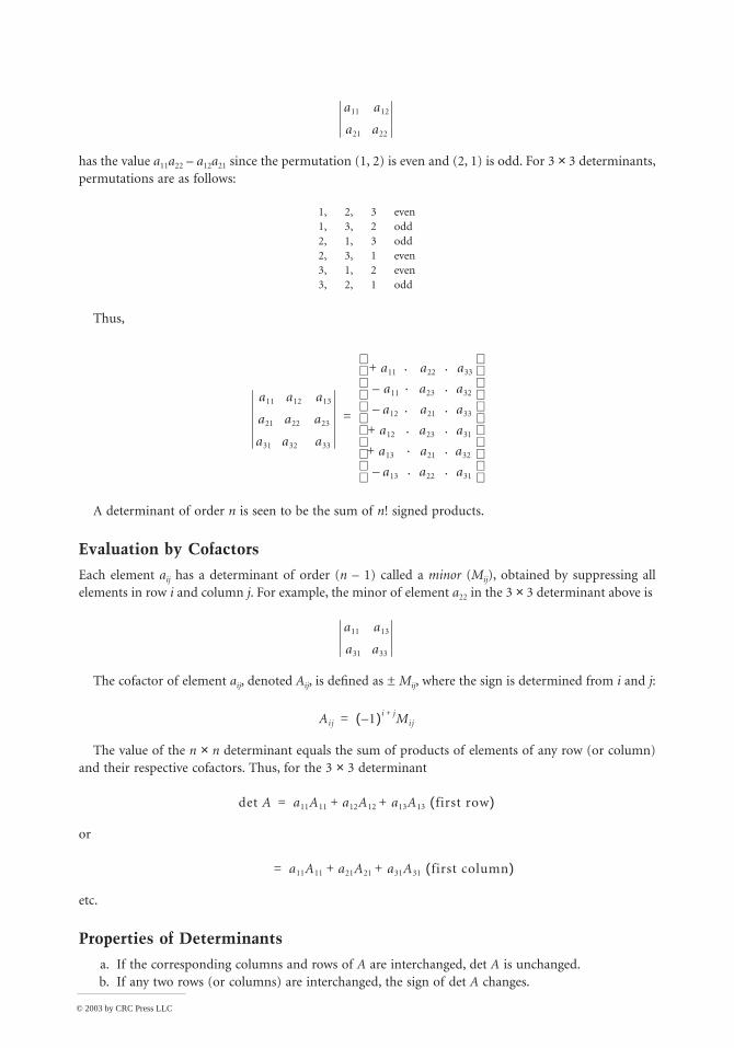
FIGURE 11 Right circular cone. V = 1/3 πR2h;
lateral surface area = πRl = πR FIGURE 12 Sphere. V = 4/3 πR3;
surface area = 4πR2.
R
hh
A
hI
R
R
R2 h2+ .
det A
a11 a12 L a1n
a21 a22 L a2n
L L L L
an1 an2 L ann
=
±( )a1ia2 ja3k K anl∑
© 2003 by CRC Press LLC
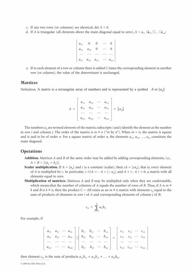
has the value a11a22 – a12a21 since the permutation (1, 2) is even and (2, 1) is odd. For 3 × 3 determinants, permutations are as follows:
Thus,
A determinant of order n is seen to be the sum of n! signed products.
Evaluation by Cofactors
Each element aij has a determinant of order (n – 1) called a minor (Mij), obtained by suppressing all elements in row i and column j. For example, the minor of element a22 in the 3 × 3 determinant above is
The cofactor of element aij, denoted Aij, is defined as ± Mij, where the sign is determined from i and j:
The value of the n × n determinant equals the sum of products of elements of any row (or column) and their respective cofactors. Thus, for the 3 × 3 determinant
or
etc.
Properties of Determinants
a. If the corresponding columns and rows of A are interchanged, det A is unchanged.b. If any two rows (or columns) are interchanged, the sign of det A changes.
1, 2, 3 even1, 3, 2 odd2, 1, 3 odd2, 3, 1 even3, 1, 2 even3, 2, 1 odd
a11 a12
a21 a22
a11 a12 a13
a21 a22 a23
a31 a32 a33
a+ 11 . a22 . a33
a– 11. a23 . a32
a12– . a21 . a33
a12+ . a23 . a31
a13+ . a21 . a32
a13– . a22 . a31
=
a11 a13
a31 a33
Aij 1–( )i j+ Mij=
det A a11A11 a12A12 a13A13 first row( )+ +=
a11A11 a21A21 a31A31 first column( )+ +=
© 2003 by CRC Press LLC
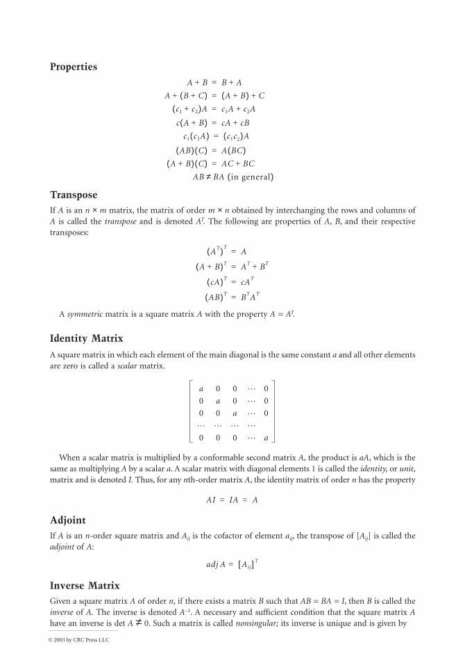
c. If any two rows (or columns) are identical, det A = 0.d. If A is triangular (all elements above the main diagonal equal to zero), A = a11 ⋅ a22 ⋅ K ⋅ ann:
e. If to each element of a row or column there is added C times the corresponding element in another row (or column), the value of the determinant is unchanged.
Matrices
Definition. A matrix is a rectangular array of numbers and is represented by a symbol A or [aij]:
The numbers aij are termed elements of the matrix; subscripts i and j identify the element as the number in row i and column j. The order of the matrix is m × n (“m by n”). When m = n, the matrix is square and is said to be of order n. For a square matrix of order n, the elements a11, a22, K, ann constitute the main diagonal.
Operations
Addition. Matrices A and B of the same order may be added by adding corresponding elements, i.e., A + B = [(aij + bij)].
Scalar multiplication. If A = [aij] and c is a constant (scalar), then cA = [caij], that is, every element of A is multiplied by c. In particular, (–1)A = – A = [– aij], and A + (– A ) = 0, a matrix with all elements equal to zero.
Multiplication of matrices. Matrices A and B may be multiplied only when they are conformable, which means that the number of columns of A equals the number of rows of B. Thus, if A is m ×k and B is k × n, then the product C = AB exists as an m × n matrix with elements cij equal to the sum of products of elements in row i of A and corresponding elements of column j of B:
For example, if
then element c21 is the sum of products a21b11 + a22b21 + K + a2kbk1.
a11 0 0 L 0
a21 a22 0 L 0
L L L L L
an1 an2 an3 L ann
A
a11 a12 L a1n
a21 a22 L a2n
L L L L
am1 am2 L amn
aij[ ]= =
cij ailblj
l 1=
k
∑=
a11 a12 L a1k
a21 a22 L a2k
L L L L
am1 L L amk
b11 b12 L b1n
b21 b22 L b2n
L L L L
bk1 bk2 L bkn
⋅
c11 c12 L c1n
c21 c22 L c2n
L L L
cm1 cm2 L cmn
=
© 2003 by CRC Press LLC
Properties
TransposeIf A is an n × m matrix, the matrix of order m × n obtained by interchanging the rows and columns of A is called the transpose and is denoted AT. The following are properties of A, B, and their respective transposes:
A symmetric matrix is a square matrix A with the property A = AT.
Identity Matrix
A square matrix in which each element of the main diagonal is the same constant a and all other elements are zero is called a scalar matrix.
When a scalar matrix is multiplied by a conformable second matrix A, the product is aA, which is the same as multiplying A by a scalar a. A scalar matrix with diagonal elements 1 is called the identity, or unit,matrix and is denoted I. Thus, for any nth-order matrix A, the identity matrix of order n has the property
AdjointIf A is an n-order square matrix and Aij is the cofactor of element aij, the transpose of [Aij] is called the adjoint of A:
Inverse MatrixGiven a square matrix A of order n, if there exists a matrix B such that AB = BA = I, then B is called theinverse of A. The inverse is denoted A–1. A necessary and sufficient condition that the square matrix A have an inverse is det A ≠ 0. Such a matrix is called nonsingular; its inverse is unique and is given by
A B+ B A+=
A B C+( )+ A B+( ) C+=
c1 c2+( )A c1A c2A+=
c A B+( ) cA cB+=
c1 c2A( ) c1c2( )A=
AB( ) C( ) A BC( )=
A B+( ) C( ) AC BC+=
AB BA in general( )≠
AT( )TA=
A B+( )T AT BT+=
cA( )T cAT=
AB( )T BTAT=
a 0 0 L 0
0 a 0 L 0
0 0 a L 0
L L L L
0 0 0 L a
AI IA A= =
adj A Aij[ ] T=
© 2003 by CRC Press LLC
Thus, to form the inverse of the nonsingular matrix A, form the adjoint of A and divide each element of the adjoint by det A. For example,
Therefore,
Systems of Linear Equations
Given the system
a unique solution exists if det A ≠ 0, where A is the n × n matrix of coefficients [aij].
Solution by Determinants (Cramer’s Rule)
where Ak is the matrix obtained from A by replacing the kth column of A by the column of bs.
A 1– adj Adet A--------------=
1 0 2
3 1– 1
4 5 6
has matrix of cofactors 11– 14– 19
10 2– 5–
2 5 1–
adjoint =11– 10 2
14– 2– 5
19 5– 1–
and determinant 27=
A 1–
11–27
--------1027-----
227-----
14–27
--------2–
27------
527-----
1927-----
5–27------
1–27------
=
a11x1 a12x2 L a1nxn b1=+ + +
a21x1 a22x2 L a2nxn b2=+ + +
M M M M Man1x1 an2x2 L annxn bn=+ + +
x1
b1 a12 L a1n
b2 a22
M M M
bn an2 ann
det A÷=
x2
a11 b1 a13 L a1n
a21 b2 L L
M M
an1 bn an3 ann
det A÷=
M
xk
det Ak
det A----------------=
© 2003 by CRC Press LLC
Matrix Solution
The linear system may be written in matrix form AX = B, where A is the matrix of coefficients [aij] and X and B are
If a unique solution exists, det A ≠ 0; hence, A–1 exists and
Trigonometry
Triangles
In any triangle (in a plane) with sides a, b, and c and corresponding opposite angles A, B, and C,
(Law of Sines)
(Law of Cosines)
(Law of Tangents)
If the vertices have coordinates (x1, y1), (x2, y2), and (x3, y3), the area is the absolute value of the expression
X
x1
x2
M
xn
B
b1
b2
M
bn
= =
X A 1– B=
aAsin
-----------b
Bsin-----------
cCsin
-----------= =
a2 b2 c2 2cb cos A–+=
a b+a b–------------
12--- A B+( )tan
12--- A B–( )tan
--------------------------------=
12--Asin
s b–( ) s c–( )bc
------------------------------= where s 12-- a b c+ +( )=
12--Acos
s s a–( )bc
-----------------=
12--Atan
s b–( ) s c–( )s s a–( )
------------------------------ =
Area 12--bc Asin=
s s a–( ) s b–( ) s c–( ) =
12--
x1 y1 1
x2 y2 1
x3 y3 1
© 2003 by CRC Press LLC
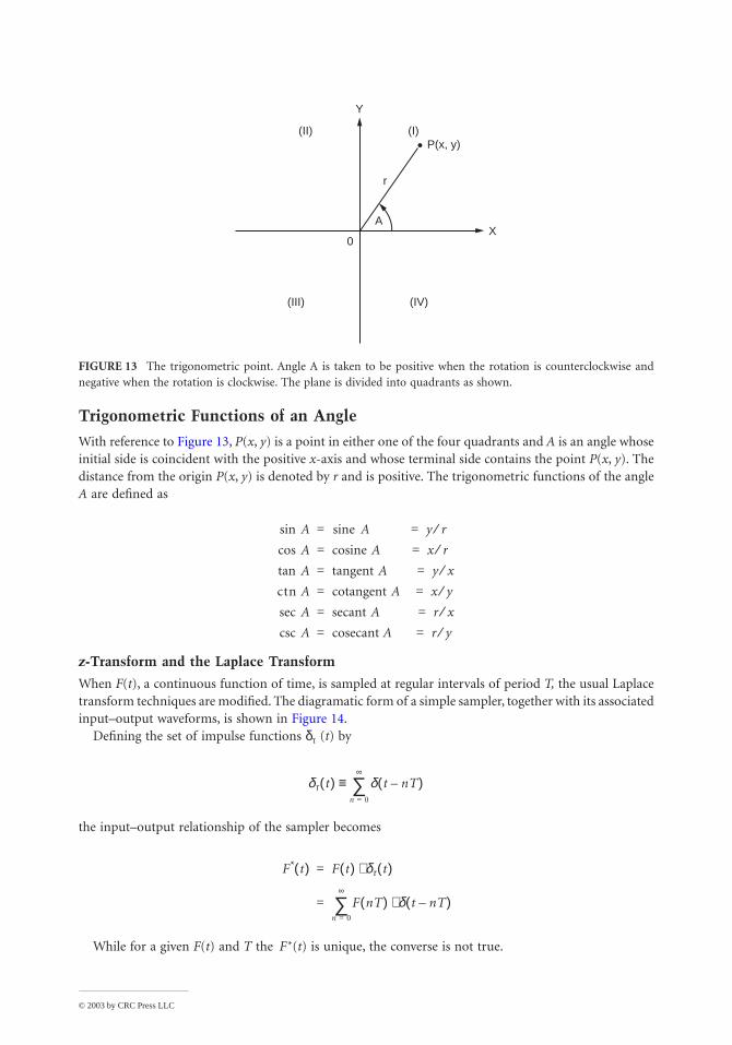
Trigonometric Functions of an Angle
With reference to Figure 13, P(x, y) is a point in either one of the four quadrants and A is an angle whose initial side is coincident with the positive x-axis and whose terminal side contains the point P(x, y). The distance from the origin P(x, y) is denoted by r and is positive. The trigonometric functions of the angle A are defined as
z-Transform and the Laplace Transform
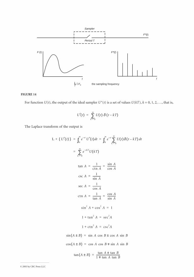
When F(t), a continuous function of time, is sampled at regular intervals of period T, the usual Laplace transform techniques are modified. The diagramatic form of a simple sampler, together with its associated input–output waveforms, is shown in Figure 14.
Defining the set of impulse functions δτ (t) by
the input–output relationship of the sampler becomes
While for a given F(t) and T the F* (t) is unique, the converse is not true.
FIGURE 13 The trigonometric point. Angle A is taken to be positive when the rotation is counterclockwise and negative when the rotation is clockwise. The plane is divided into quadrants as shown.
Y
XA
0
P(x, y)
r
(I)(II)
(III) (IV)
Asin e A sin y r⁄= =
Acos cosine A x r⁄= =
Atan tangent A y x⁄= =
ctn A cotangent A x y⁄= =
sec A secant A r x⁄= =
csc A cosecant A r y⁄= =
δτ t( ) δ t nT–( )n 0=
∞
∑≡
F* t( ) F t( ) δτ t( )⋅=
F nT( ) δ t nT–( )⋅n 0=
∞
∑=
© 2003 by CRC Press LLC
For function U(t), the output of the ideal sampler U*(t) is a set of values U(kT ), k = 0, 1, 2, …, that is,
The Laplace transform of the output is
FIGURE 14
Sampler
Period T
F*(t)F (t)
F*(t)
tt
the sampling frequency1T ≡Fs
U* t( ) U t( ) δ t kT–( )k 0=
∞
∑=
L + U* t( ) e st– U* t( ) td0
∞
∫ e st– U t( )δ t kT–( )k 0=
∞
∑ td0
∞
∫= =
e skT– U kT( )k 0=
∞
∑=
Atan1
ctn A--------------
Asin Acos
--------------= =
Acsc1 Asin
-------------=
Asec1
cos A--------------=
ctn A1
tan A--------------
cos A sin A
--------------= =
sin2 A cos2 A+ 1=
1 tan2 A+ sec2A=
1 ctn2 A+ csc2A=
A B±( )sin A B A cos± Bsincossin=
A B±( )cos Acos B Asin +− Bsincos=
A B±( )tan Atan Btan±
1 A Btantan+−---------------------------------------=
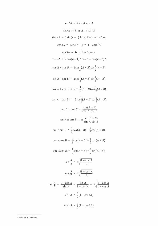
© 2003 by CRC Press LLC
2Asin 2 A Acossin=
3Asin 3 A 4sin3 A–sin=
nAsin 2 n 1–( )A A n 2–( )Asin–cossin=
2Acos 2cos2A 1– 1 2sin2A–= =
3Acos 4cos3A 3 Acos–=
nAcos 2 n 1–( )A A n 2–( )Acos–coscos=
A Bsin+sin 2 12-- A B+( ) 1
2-- A B–( )cossin=
A Bsin–sin 212--cos A B+( ) 1
2--sin A B–( )=
A Bcos+cos 212--cos A B+( ) 1
2--cos A B–( )=
A Bcos–cos 2–12--sin A B+( ) 1
2--sin A B–( )=
A Btan±tanA B±( )sin
A Bcoscos------------------------------=
ctn A ctn B± A B±( )sin sin A sin B
----------------------------±=
A Bsinsin 12-- A B–( )cos 1
2--– A B+( )cos=
cos A Bcos 12-- A B–( )cos 1
2-- A B+( )cos+=
A Bcossin 12-- A B+( )sin 1
2-- A B–( )sin+=
A2---sin
1 Acos–2
-----------------------±=
A2---cos
1 Acos+2
-----------------------±=
A2---tan
1 Acos– Asin
----------------------- Asin
1 Acos+-----------------------
1 Acos–1 Acos+-----------------------±= = =
sin2 A 12-- 1 2Acos–( )=
cos2 A 12-- 1 2Acos+( )=
© 2003 by CRC Press LLC
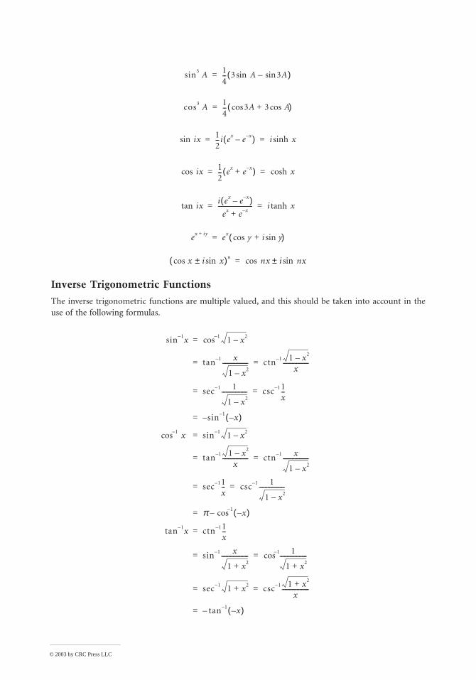
Inverse Trigonometric Functions
The inverse trigonometric functions are multiple valued, and this should be taken into account in the use of the following formulas.
sin3 A 14-- 3 A 3Asin–sin( )=
cos3 A 14-- 3A 3 Acos+cos( )=
ixsin 12--i ex e x––( ) i xsinh= =
icos x 12-- ex e x–+( ) xcosh= =
ixtani ex e x––( )
ex e x–+----------------------- i xtanh= =
ex iy+ ex y i ysin+cos( )=
x i xsin±cos( )n nx i nxsin±cos=
sin 1– x 1– 1 x2–cos=
tan 1– x
1 x2–----------------- ctn 1– 1 x2–
x-----------------= =
sec 1– 1
1 x2–----------------- csc 1– 1
x--= =
s– in 1– x–( )=
1– xcos sin 1– 1 x2–=
tan 1– 1 x2–x
----------------- ctn 1– x
1 x2–-----------------= =
sec 1– 1x-- csc 1– 1
1 x2–-----------------= =
π 1– x–( )cos–=
tan 1– x ctn 1– 1x--=
sin 1– x
1 x2+------------------
1– 1
1 x2+------------------cos= =
sec 1– 1 x2+ csc 1– 1 x2+x
------------------= =
t– an 1– x–( )=
© 2003 by CRC Press LLC
Analytic Geometry
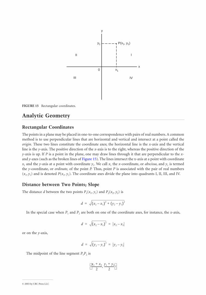
Rectangular Coordinates
The points in a plane may be placed in one-to-one correspondence with pairs of real numbers. A common method is to use perpendicular lines that are horizontal and vertical and intersect at a point called theorigin. These two lines constitute the coordinate axes; the horizontal line is the x-axis and the vertical line is the y-axis. The positive direction of the x-axis is to the right, whereas the positive direction of the y-axis is up. If P is a point in the plane, one may draw lines through it that are perpendicular to the x- and y-axes (such as the broken lines of Figure 15). The lines intersect the x-axis at a point with coordinate x1 and the y-axis at a point with coordinate y1. We call x1 the x-coordinate, or abscissa, and y1 is termed the y-coordinate, or ordinate, of the point P. Thus, point P is associated with the pair of real numbers (x1, y1) and is denoted P(x1, y1). The coordinate axes divide the plane into quadrants I, II, III, and IV.
Distance between Two Points; Slope
The distance d between the two points P1(x1, y1) and P2(x2, y2) is
In the special case when P1 and P2 are both on one of the coordinate axes, for instance, the x-axis,
or on the y-axis,
The midpoint of the line segment P1P2 is
FIGURE 15 Rectangular coordinates.
y
x
IV
III
III
0
y1
x1
P(x1, y1)
d x2 x1–( )2 y2 y1–( )2+=
d x2 x1–( )2 x2 x1–= =
d y2 y1–( )2 y2 y1–= =
x1 x2+2
----------------y1 y2+
2---------------,
© 2003 by CRC Press LLC
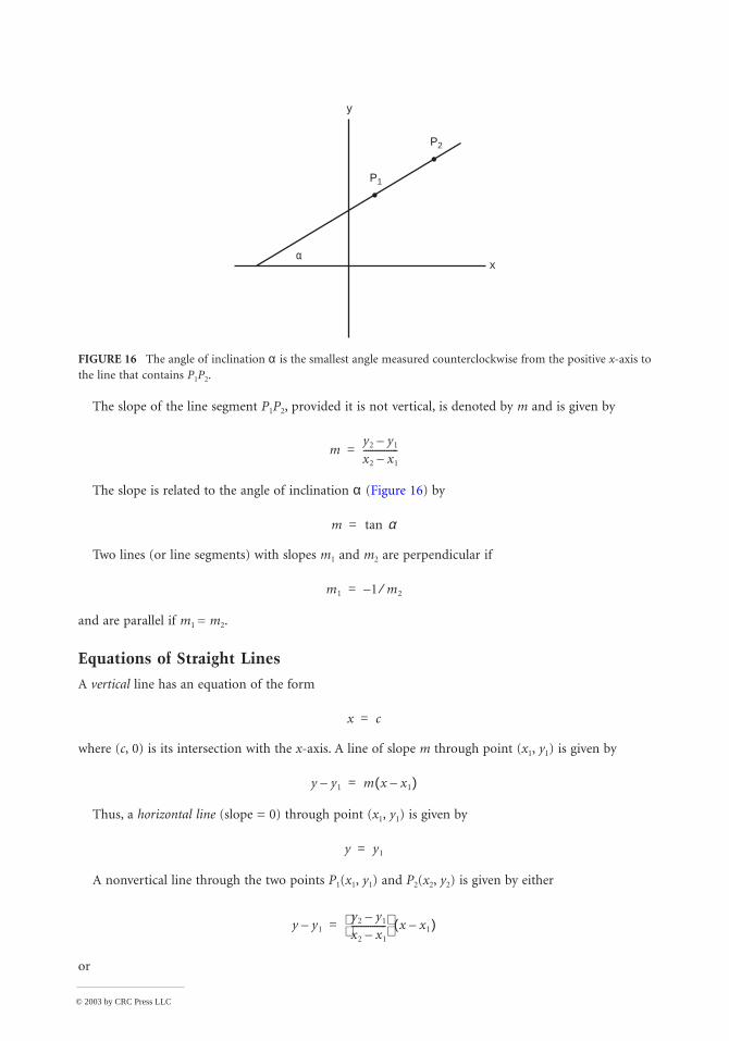
The slope of the line segment P1P2, provided it is not vertical, is denoted by m and is given by
The slope is related to the angle of inclination α (Figure 16) by
Two lines (or line segments) with slopes m1 and m2 are perpendicular if
and are parallel if m1 = m2.
Equations of Straight Lines
A vertical line has an equation of the form
where (c, 0) is its intersection with the x-axis. A line of slope m through point (x1, y1) is given by
Thus, a horizontal line (slope = 0) through point (x1, y1) is given by
A nonvertical line through the two points P1(x1, y1) and P2(x2, y2) is given by either
or
FIGURE 16 The angle of inclination α is the smallest angle measured counterclockwise from the positive x-axis to the line that contains P1P2.
y
x
P1
P2
α
my2 y1–x2 x1–---------------=
m αtan=
m1 1 m2⁄–=
x c=
y y1– m x x1–( )=
y y1=
y y1–y2 y1–x2 x1–---------------
x x1–( )=
© 2003 by CRC Press LLC
A line with x-intercept a and y-intercept b is given by
The general equation of a line is
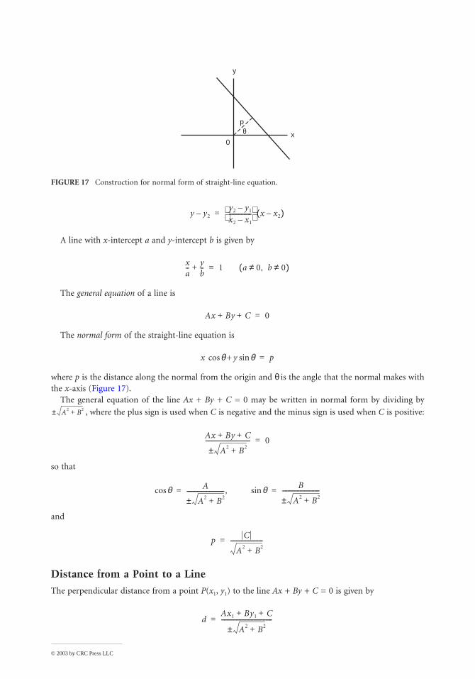
The normal form of the straight-line equation is
where p is the distance along the normal from the origin and θ is the angle that the normal makes with the x-axis (Figure 17).
The general equation of the line Ax + By + C = 0 may be written in normal form by dividing by
, where the plus sign is used when C is negative and the minus sign is used when C is positive:
so that
and
Distance from a Point to a Line
The perpendicular distance from a point P(x1, y1) to the line Ax + By + C = 0 is given by
FIGURE 17 Construction for normal form of straight-line equation.
y
x0
pθ
y y2–y2 y1–x2 x1–---------------
x x2–( )=
xa--
yb--+ 1 a 0 b 0≠,≠( )=
Ax By C+ + 0=
x θ + y θsincos p=
A2 B2+±
Ax By C+ +
A2 B2+±------------------------------ 0=
θcos A
A2 B2+±------------------------- θsin, B
A2 B2+±-------------------------= =
pC
A2 B2+----------------------=
dAx1 By1 C+ +
A2 B2+±----------------------------------=
© 2003 by CRC Press LLC
Circle
The general equation of a circle of radius r and center at P(x1, y1) is
Parabola
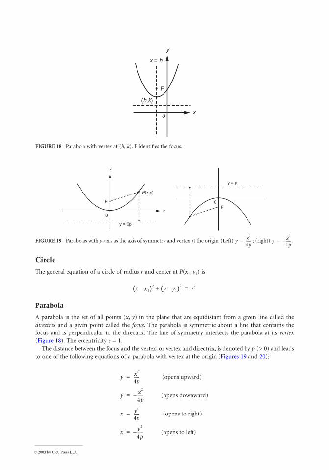
A parabola is the set of all points (x, y) in the plane that are equidistant from a given line called the directrix and a given point called the focus. The parabola is symmetric about a line that contains the focus and is perpendicular to the directrix. The line of symmetry intersects the parabola at its vertex(Figure 18). The eccentricity e = 1.
The distance between the focus and the vertex, or vertex and directrix, is denoted by p (> 0) and leads to one of the following equations of a parabola with vertex at the origin (Figures 19 and 20):
FIGURE 18 Parabola with vertex at (h, k). F identifies the focus.
FIGURE 19 Parabolas with y-axis as the axis of symmetry and vertex at the origin. (Left) ; (right)
xo
F
y
x = h
(h,k)
F
0
0F
y = p
y = −p
x
y
P(x,y)
y x2
4p------= y x2
4p------– .=
x x1–( )2 y y1–( )2+ r2=
y x2
4p------ (opens upward)=
y x2
4p------ (opens downward)–=
x y2
4p------ (opens to right)=
x y2
4p------ (opens to left)–=
© 2003 by CRC Press LLC
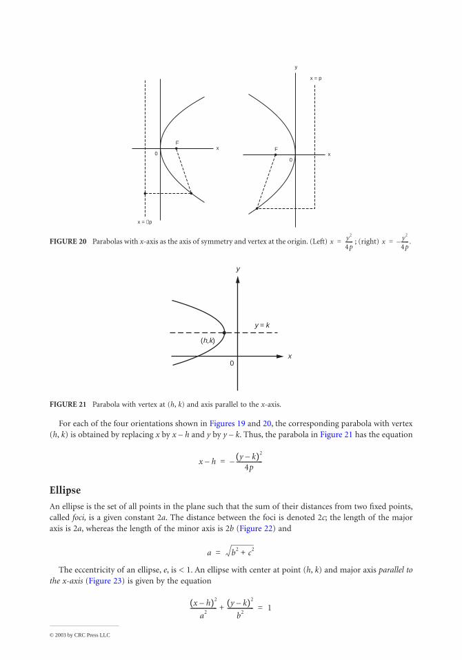
For each of the four orientations shown in Figures 19 and 20, the corresponding parabola with vertex (h, k) is obtained by replacing x by x – h and y by y – k. Thus, the parabola in Figure 21 has the equation
Ellipse
An ellipse is the set of all points in the plane such that the sum of their distances from two fixed points, called foci, is a given constant 2a. The distance between the foci is denoted 2c; the length of the major axis is 2a, whereas the length of the minor axis is 2b (Figure 22) and
The eccentricity of an ellipse, e, is < 1. An ellipse with center at point (h, k) and major axis parallel to the x-axis (Figure 23) is given by the equation
FIGURE 20 Parabolas with x-axis as the axis of symmetry and vertex at the origin. (Left) ; (right)
FIGURE 21 Parabola with vertex at (h, k) and axis parallel to the x-axis.
y
x = p
x0
FxF
0
x = −p
x y2
4p------= x y2
4p------– .=
0x
(h,k)
y
y = k
x h–y k–( )2
4p------------------–=
a b2 c2+=
x h–( )2
a2------------------
y k–( )2
b2------------------+ 1=
© 2003 by CRC Press LLC
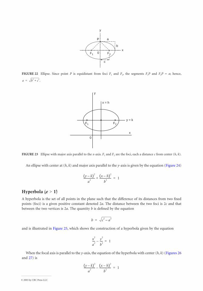
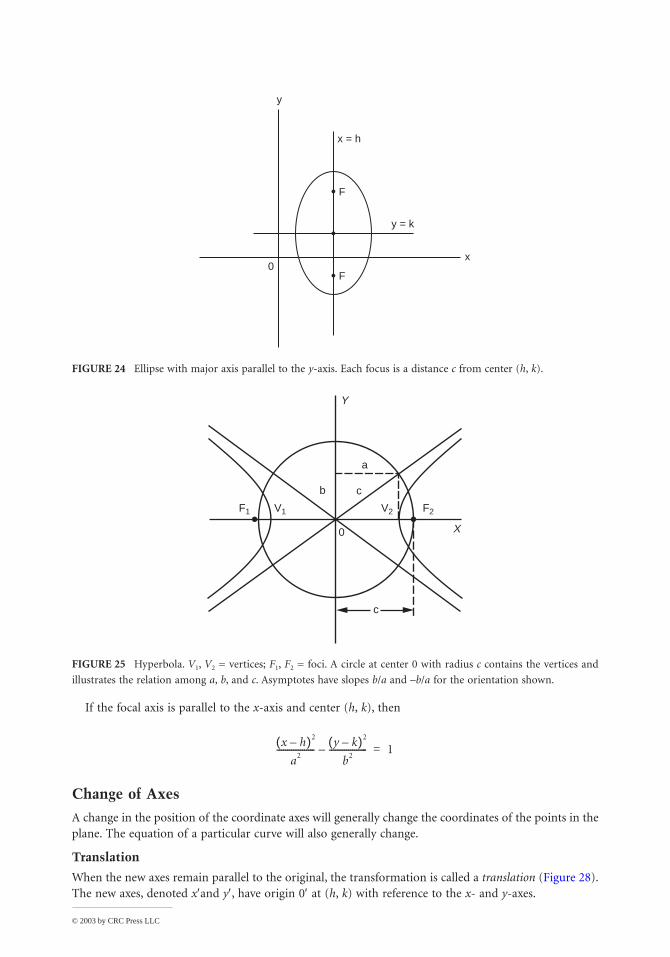
An ellipse with center at (h, k) and major axis parallel to the y-axis is given by the equation (Figure 24)
Hyperbola (e > 1)
A hyperbola is the set of all points in the plane such that the difference of its distances from two fixed points (foci) is a given positive constant denoted 2a. The distance between the two foci is 2c and that between the two vertices is 2a. The quantity b is defined by the equation
and is illustrated in Figure 25, which shows the construction of a hyperbola given by the equation
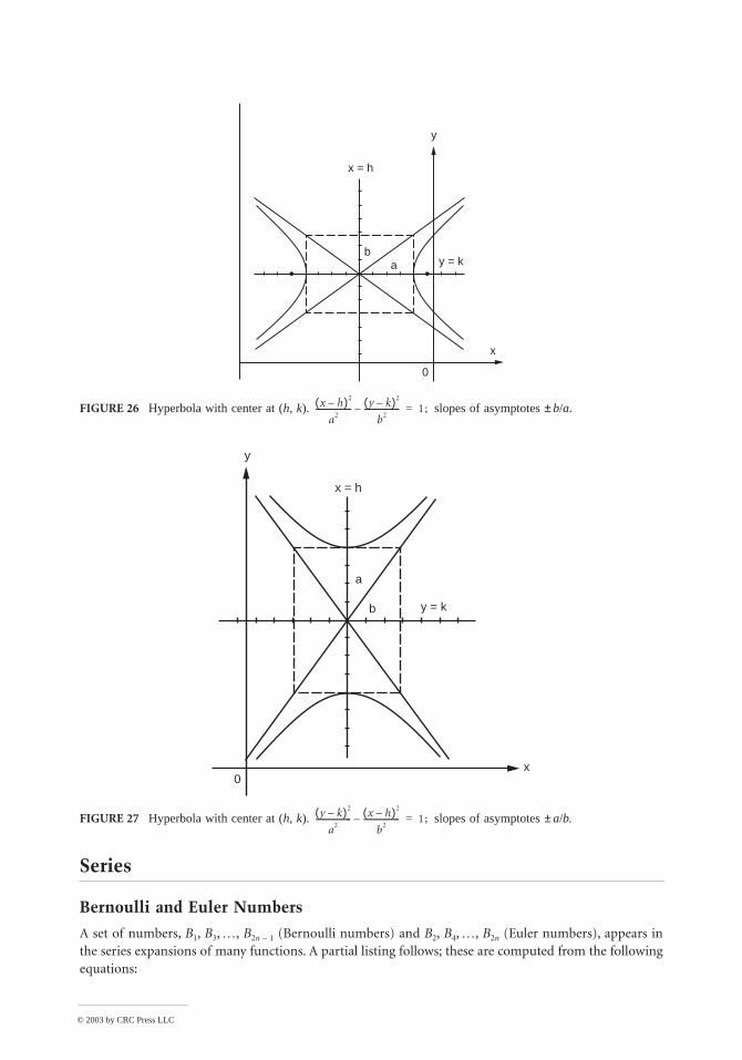
When the focal axis is parallel to the y-axis, the equation of the hyperbola with center (h, k) (Figures 26 and 27) is
FIGURE 22 Ellipse. Since point P is equidistant from foci F1 and F2, the segments F1P and F2P = a; hence,
FIGURE 23 Ellipse with major axis parallel to the x-axis. F1 and F2 are the foci, each a distance c from center (h, k).
x
y
b
aP
c
0 F2F1
a b2 c2+ .=
F2F1
y = k
x
0
x = h
y
y k–( )2
a2------------------
x h–( )2
b2------------------+ 1=
b c2 a2–=
x2
a2----
y2
b2----– 1=
y k–( )2
a2------------------
x h–( )2
b2------------------– 1=
© 2003 by CRC Press LLC
If the focal axis is parallel to the x-axis and center (h, k), then
Change of Axes
A change in the position of the coordinate axes will generally change the coordinates of the points in the plane. The equation of a particular curve will also generally change.
Translation
When the new axes remain parallel to the original, the transformation is called a translation (Figure 28). The new axes, denoted x′and y′, have origin 0′ at (h, k) with reference to the x- and y-axes.
FIGURE 24 Ellipse with major axis parallel to the y-axis. Each focus is a distance c from center (h, k).
FIGURE 25 Hyperbola. V1, V2 = vertices; F1, F2 = foci. A circle at center 0 with radius c contains the vertices and
illustrates the relation among a, b, and c. Asymptotes have slopes b/a and –b/a for the orientation shown.
F
F
0x
y = k
x = h
y
X
Y
b
a
c
0
c
V1F1 V2 F2
x h–( )2
a2------------------
y k–( )2
b2------------------– 1=
© 2003 by CRC Press LLC
Series
Bernoulli and Euler Numbers
A set of numbers, B1, B3, K, B2n – 1 (Bernoulli numbers) and B2, B4, K, B2n (Euler numbers), appears in the series expansions of many functions. A partial listing follows; these are computed from the following equations:
FIGURE 26 Hyperbola with center at (h, k). slopes of asymptotes ± b/a.
FIGURE 27 Hyperbola with center at (h, k). slopes of asymptotes ± a/b.
x = h
ba y = k
0
x
y
x h–( )2
a2------------------ y k–( )2
b2------------------– 1;=
y
x = h
a
b y = k
x0
y k–( )2
a2------------------ x h–( )2
b2------------------– 1;=

© 2003 by CRC Press LLC
and
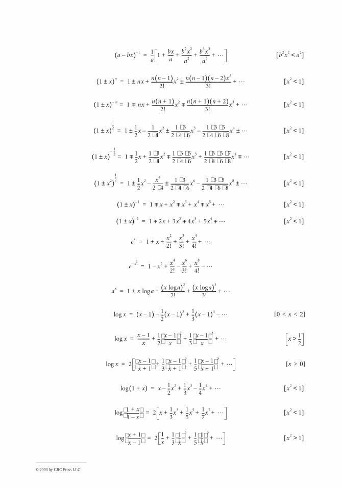
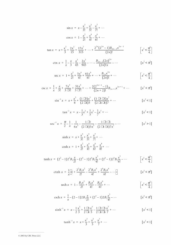
Series of Functions
In the following, the interval of convergence is indicated; otherwise, it is all x. Logarithms are of base e. Bernoulli and Euler numbers (B2n – 1 and B2n) appear in certain expressions.
FIGURE 28 Translation of axes.
y
0
P
y′
x′
x
0′ (h, k)
B2n2n 2n 1–( )
2!--------------------------B2n 2–– 2n 2n 1–( ) 2n 2–( ) 2n 3–( )
4!-------------------------------------------------------------------B2n 4– L– 1–( )n+ + 0=
22n 22n 1–( )2n
----------------------------B2n 1– 2n 1–( )B2n 2–2n 1–( ) 2n 2–( ) 2n 3–( )
3!------------------------------------------------------------B2n 4–– L 1–( )n 1–+ +=
B1 1 6⁄ B2 1= =
B3 1 30⁄ B4 5= =
B5 1 42⁄ B6 61= =
B7 1 30⁄ B8 1385= =
B9 5 66⁄ B10 50,521= =
B11 691 2730⁄ B12 2,702,765= =
B13 7 6⁄ B14 199,360,981= =
M M
a x+( )n an nan 1– x n n 1–( )2!
--------------------an 2– x2 n n 1–( ) n 2–( )3!
-------------------------------------an 3– x3L
n!n j–( )!j!
---------------------an j– x jL
+ + + +
+ +
= x2 a2<[ ]
© 2003 by CRC Press LLC
[0 < x < 2]
[x > 0]
a bx–( ) 1– 1a-- 1
bxa
-----b2x2
a2---------
b3x3
a3--------- L+ + + += b2x2 a2<[ ]
1 x±( )n 1 nx± n n 1–( )2!
--------------------x2 n n 1–( ) n 2–( )x3
3!------------------------------------------± L+ += x2 1<[ ]
1 x±( ) n– 1 nx+− n n 1+( )2!
---------------------x2 n n 1+( ) n 2+( )3!
--------------------------------------x3+− L+ += x2 1<[ ]
1 x±( )12--
1 12--x± 1
2 4⋅----------x2– 1 3⋅
2 4 6⋅ ⋅-----------------x3± 1 3 5⋅ ⋅
2 4 6 8⋅ ⋅ ⋅-------------------------x4– L±= x2 1<[ ]
1 x±( )12--–
1 12--x+− 1 3⋅
2 4⋅----------x2 1 3 5⋅ ⋅
2 4 6⋅ ⋅-----------------x3+− 1 3 5 7⋅ ⋅ ⋅
2 4 6 8⋅ ⋅ ⋅-------------------------x4
L+−+ += x2 1<[ ]
1 x2±( )12--
1 12--x2± x4
2 4⋅----------– 1 3⋅
2 4 6⋅ ⋅-----------------x6± 1 3 5⋅ ⋅
2 4 6 8⋅ ⋅ ⋅-------------------------x8– L±= x2 1<[ ]
1 x±( ) 1– 1 x+− x2 x3+− x4 x5+− L+ + += x2 1<[ ]
1 x±( ) 2– 1 2x+− 3x2 4x3+− 5x4L+−+ += x2 1<[ ]
ex 1 xx2
2!----
x3
3!----
x4
4!---- L+ + + + +=
e x2
– 1 x2–x4
2!----
x6
3!----–
x8
4!---- L–+ +=
ax 1 x alogx alog( )2
2!----------------------
x alog( )3
3!---------------------- L+ + + +=
xlog x 1–( ) 12-- x 1–( )2– 1
3-- x 1–( )3
L–+=
xlogx 1–
x----------- 1
2--
x 1–x
----------- 2 1
3--
x 1–x
----------- 3
L+ + += x 12-->
xlog 2 x 1–x 1+------------
13--
x 1–x 1+------------
3 15--
x 1–x 1+------------
5
L+ + +=
1 x+( )log x 12--x2– 1
3--x3 1
4--x4– L+ += x2 1<[ ]
1 x+1 x–------------
log 2 x 13--x3 1
5--x5 1
7--x7
L+ + + += x2 1<[ ]
x 1+x 1–------------
log 21x-- 1
3--
1x--
3 15--
1x--
5
L+ + += x2 1>[ ]
© 2003 by CRC Press LLC
xsin xx3
3!----–
x5
5!----
x7
7!----– L+ +=
xcos 1x2
2!----–
x4
4!----
x6
6!----– L+ +=
xtan xx3
3----
2x5
15--------
17x7
315---------- L
22n 22n 1–( )B2n 1– x2n 1–
2n( )!------------------------------------------------------+ + + + += x2 π2
4-----<
ctn x1x--
x3--–
x3
45-----–
2x5
945--------– L–
B2n 1– 2x( )2n
2n( )!x----------------------------– L–= x2 π2<[ ]
xsec 1x2
2!----
5x4
4!--------
61x6
6!---------- L
B2nx2n
2n( )!--------------- L+ + + + + += x2 π2
4-----<
xcsc1x--
x3!----
7x3
3 5!⋅------------
31x5
3 7!⋅------------ L
2 22n 1+ 1–( )2n 2+( )!
-----------------------------B2n 1+ x2n 1+L+ + + + + += x2 π2<[ ]
sin 1– x xx3
6----
1 3⋅( )x5
2 4⋅( )5--------------------
1 3 5⋅ ⋅( )x7
2 4 6⋅ ⋅( )7--------------------------- L+ + + += x2 1<[ ]
tan 1– x x 13--x3– 1
5--x5 1
7--x7– L+ += x2 1<[ ]
sec 1– xπ2---
1x--–
1
6x3--------–
1 3⋅2 4⋅( )5x5
-----------------------–1 3 5⋅ ⋅
2 4 6⋅ ⋅( )7x7------------------------------– L–= x2 1>[ ]
xsinh xx3
3!----
x5
5!----
x7
7!---- L+ + + +=
xcosh 1x2
2!----
x4
4!----
x6
6!----
x8
8!---- L+ + + + +=
xtanh 22 1–( )22B1x2!---- 24 1–( )24B3
x3
4!----– 26 1–( )26B5
x5
6!---- L–+= x2 π2
4-----<
ctnh x 1x-- 1
22B1x2
2!---------------
24B3x4
4!---------------–
26B5x6
6!--------------- L–+ +
= x2 π2<[ ]
xsech 1B2x2
2!----------–
B4x4
4!----------
B6x6
6!----------– L+ += x2 π2
4-----<
xcsch1x-- 2 1–( )2B1
x2!----– 23 1–( )2B3
x3
4!---- L–+= x2 π2<[ ]
sinh 1– x x 12--
x3
3----– 1 3⋅
2 4⋅----------
x5
5----
1 3 5⋅ ⋅2 4 6⋅ ⋅-----------------
x7
7----– L+ += x2 1<[ ]
tanh 1– x xx3
3----
x5
5----
x7
7---- L+ + + += x2 1<[ ]
© 2003 by CRC Press LLC
Error Function
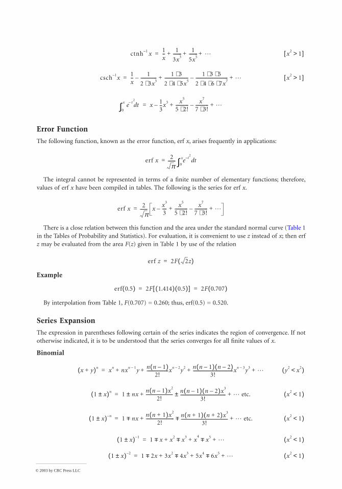
The following function, known as the error function, erf x, arises frequently in applications:
The integral cannot be represented in terms of a finite number of elementary functions; therefore, values of erf x have been compiled in tables. The following is the series for erf x.
There is a close relation between this function and the area under the standard normal curve (Table 1 in the Tables of Probability and Statistics). For evaluation, it is convenient to use z instead of x; then erf z may be evaluated from the area F(z) given in Table 1 by use of the relation
Example
By interpolation from Table 1, F(0.707) = 0.260; thus, erf(0.5) = 0.520.
Series Expansion
The expression in parentheses following certain of the series indicates the region of convergence. If not otherwise indicated, it is to be understood that the series converges for all finite values of x.
Binomial
ctnh 1– x1x--
1
3x3--------
1
5x5-------- L+ + += x2 1>[ ]
csch 1– x1x--
1
2 3x3⋅---------------–
1 3⋅2 4 5x5⋅ ⋅----------------------
1 3 5⋅ ⋅2 4 6 7x7⋅ ⋅ ⋅------------------------------– L+ += x2 1>[ ]
e t2
– td0
x
∫ x 13--x3–
x5
5 2!⋅------------
x7
7 3!⋅------------– L+ +=
erf x 2
π------- e t
2– td
0
x∫=
erf x 2
π------- x
x3
3----–
x5
5 2!⋅------------
x7
7 3!⋅------------– L+ +=
erf z 2F 2z( )=
erf 0.5( ) 2F 1.414( ) 0.5( )[ ] 2F 0.707( )= =
x y+( )n xn nxn 1– y n n 1–( )2!
--------------------xn 2– y2 n n 1–( ) n 2–( )3!
-------------------------------------xn 3– y3L+ + + += y2 x2<( )
1 x±( )n 1 nx± n n 1–( )x2
2!------------------------- n n 1–( ) n 2–( )x3
3!------------------------------------------± L etc.+ += x2 1<( )
1 x±( ) n– 1 nx+−n n 1+( )x2
2!-------------------------- n n 1+( ) n 2+( )x3
3!--------------------------------------------+− L etc.+ += x2 1<( )
1 x±( ) 1– 1 x+− x2 x3 x+4
+− x5+− L+ += x2 1<( )
1 x±( ) 2– 1 2x+− 3x2 4x3+− 5x4 6x5+− L+ + += x2 1<( )
© 2003 by CRC Press LLC
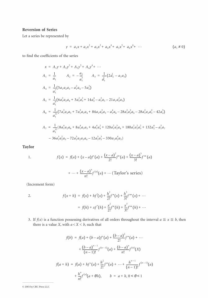
Reversion of Series
Let a series be represented by
to find the coefficients of the series
Taylor
1.
(Taylor’s series)
(Increment form)
2.
3. If f(x) is a function possessing derivatives of all orders throughout the interval a x b, then there is a value X, with a < X < b, such that
y a1x a2x2 a3x3 a4x4 a5x5 a6x6L+ + + + + += a1 0≠( )
x A1y A2y2 A3y3 A4y4L+ + + +=
A11a1
---- A2a2
a13
---- A3– 1
a15
------ 2a22 a1a3–( )= = =
A41
a17
---- 5a1a2a3 a12a4– 5a2
3–( )=
A51
a19
---- 6a12a2a4 3a1
2a32 14a2
4 a13a5– 21a1a2
2a3–+ +( )=
A61
a111
------ 7a13a2a5 7a1
3a3a4 84a1a23a3 a1
4a6– 28a12a2
2a4– 28a12a2a3
2– 42a25–+ +( )=
A71
a113
------(8a14a2a6 8a1
4a3a5 4a14a4
2 120a12a2
3a4 180a12a2
2a32 132a2
6 a15a7–+ + + + +=
36a13a2
2a5– 72a13a2a3a4– 12a1
3a33– 330a1a2
4a3)–
f x( ) f a( ) x a–( )f ′ a( ) x a–( )2
2!------------------f ″ a( ) x a–( )3
3!------------------f ′″ a( )+ + +=
Lx a–( )n
n!------------------f n( ) a( ) L+ + +
f x h+( ) f x( ) hf ′ x( ) h2
2!-----f ″ x( ) h3
3!-----f ′″ x( ) L+ + + +=
f h( ) xf ′ h( ) x2
2!----f ″ h( ) x3
3!----f ′″ h( ) L+ + + +=
f b( ) f a( ) b a–( )f ′ a( ) b a–( )2
2!------------------f ″ a( ) L+ + +=
b a–( )n 1–
n 1–( )!------------------------ f n 1–( ) a( ) b a–( )n
n!------------------f n( ) X( )+ +
f a h+( ) f a( ) hf ′ a( ) h2
2!----- f ″ a( ) L hn 1–
n 1–( )!------------------ f n 1–( ) a( )+ + + +=
hn
n!-----f n( ) a θh+( ) b,+ a h 0 θ 1< <,+=
© 2003 by CRC Press LLC
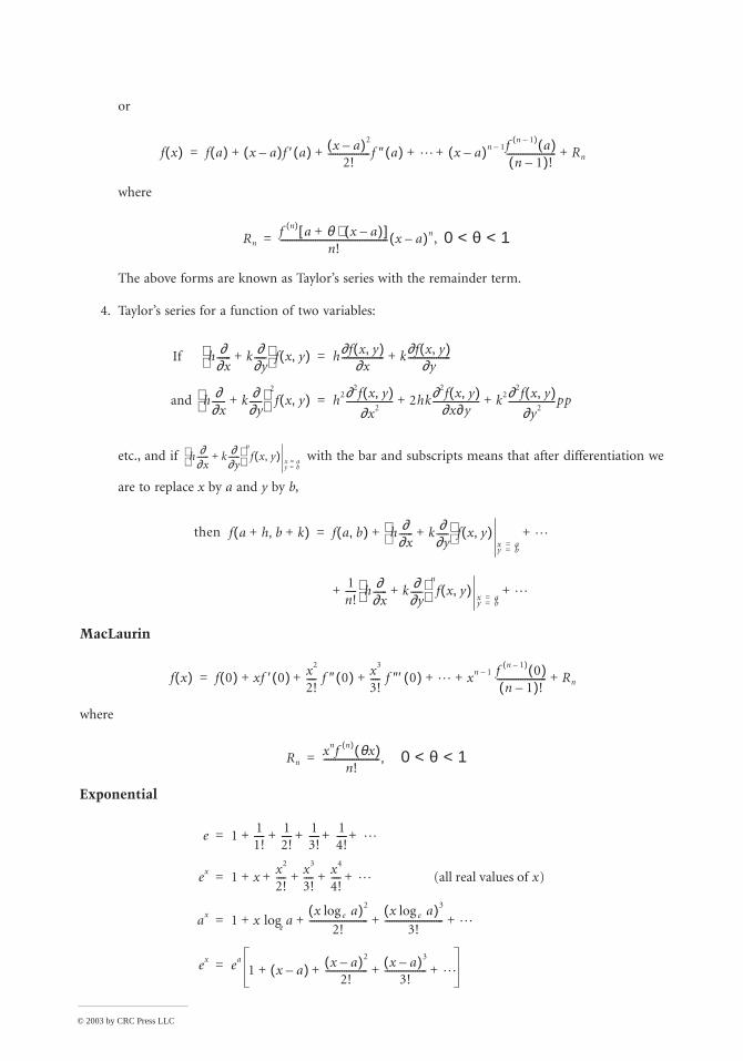
or
where
0 < θ < 1
The above forms are known as Taylor’s series with the remainder term.
4. Taylor’s series for a function of two variables:
etc., and if with the bar and subscripts means that after differentiation we
are to replace x by a and y by b,
then
MacLaurin
where
0 < θ < 1
Exponential
f x( ) f a( ) x a–( )f ′ a( ) x a–( )2
2!------------------f ″ a( ) L x a–( )n 1– f n 1–( ) a( )
n 1–( )!--------------------- Rn+ + + + +=
Rnf n( ) a θ x a–( )⋅+[ ]
n!---------------------------------------------- x a–( )n,=
If h ∂∂x------ k ∂
∂y-----+
f x y,( ) h∂f x y,( )∂x
------------------ k∂f x y,( )∂y
------------------+=
and h ∂∂x------ k ∂
∂y-----+
2
f x y,( ) h2∂2f x y,( )∂x2
-------------------- 2hk∂2f x y,( )∂x∂y
-------------------- k2∂2f x y,( )∂y2
--------------------pp+ +=
h ∂∂x------ k ∂
∂y------+
n
f x y,( )y b=x a=
f a h b k+,+( ) f a b,( ) h ∂∂x------ k ∂
∂y-----+
f x y,( )x a=y b=
L+ +=
1n!-----+ h ∂
∂x------ k ∂
∂y-----+
n
f x y,( )x a=y b=
L+
f x( ) f 0( ) xf ′ 0( ) x2
2!---- f ″ 0( ) x3
3!---- f ″′ 0( ) L x+ n 1– f n 1–( ) 0( )
n 1–( )!--------------------- Rn+ + + + +=
Rnxnf n( ) θx( )
n!------------------------,=
e 111!----
12!----
13!----
14!---- L+ + + + +=
ex 1 xx2
2!----
x3
3!----
x4
4!---- L (all real values of x)+ + + + +=
ax 1 x ax aelog( )2
2!-------------------------+
e
x aelog( )3
3!-------------------------+ L+log+=
ex ea
1 x a–( ) x a–( )2
2!------------------
x a–( )3
3!------------------ L+ + + +=
© 2003 by CRC Press LLC
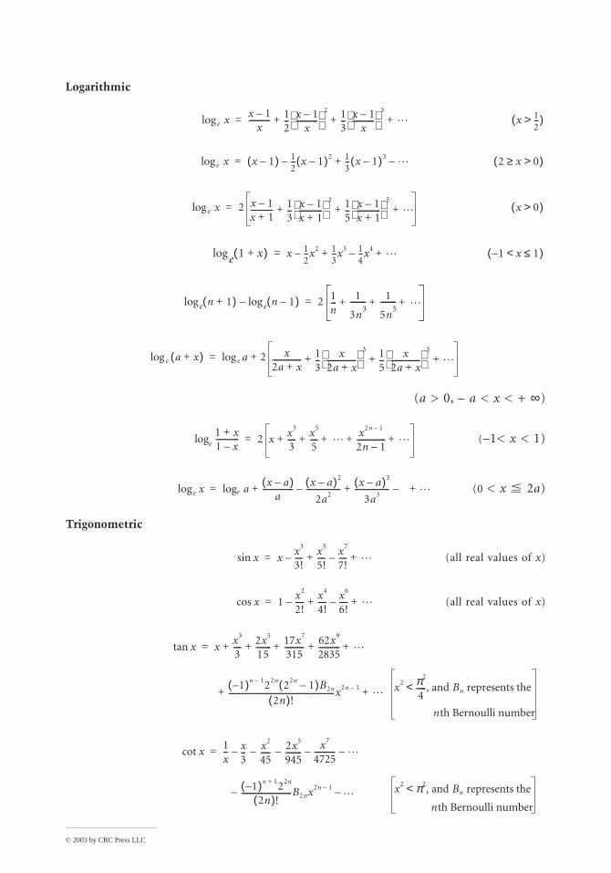
Logarithmic
(a > 0, – a < x < + ∞)
(–1< x < 1)
(0 < x 2a)
Trigonometric
(all real values of x)
(all real values of x)
xelogx 1–
x----------- 1
2--
x 1–x
----------- 2 1
3--
x 1–x
----------- 3
L+ + += x 12--->( )
xelog x 1–( ) 12--- x 1–( )2– 1
3--- x 1–( )3
L–+= 2 x 0>≥( )
xelog 2 x 1–x 1+------------ 1
3--
x 1–x 1+------------
3 15--
x 1–x 1+------------
5
L+ + += x 0>( )
1 x+( )elog x 12---x2– 1
3---x3 1
4---x4– L+ += 1– x 1≤<( )
n 1+( )e n 1–( )elog–log 2 1n---
1
3n3
------- 1
5n5
------- L+ + +=
a x+( )elog ae 2 x2a x+--------------- 1
3--
x2a x+---------------
3 15--
x2a x+---------------
5
L+ + ++log=
1 x+1 x–------------elog 2 x
x3
3----
x5
5---- L
x2n 1–
2n 1–--------------- L+ + + + +=
xelog ax a–( )
a----------------
x a–( )2
2a2------------------–
x a–( )3
3a3------------------ –+ +elog L+=
xsin xx3
3!----
x5
5!----
x7
7!----– L+ +–=
xcos 1x2
2!----
x4
4!----
x6
6!----– L+ +–=
xtan xx3
3----
2x5
15--------
17x7
315----------
62x9
2835----------- L+ + + ++=
1–( )n 1– 22n 22n 1–( )B2n
2n( )!-------------------------------------------------------x2n 1–
L x2 π2
4----- and Bn represents the ,<
nth Bernoulli number
+ +
xcot1x-- x
3-- x2
45----- – 2x5
945--------–
x7
4725-----------– L––=
1–( )n 1+ 22n
2n( )!--------------------------– B2nx2n 1–
L x2 π2 and Bn represents the ,<nth Bernoulli number
–
© 2003 by CRC Press LLC
Differential Calculus
Notation
For the following equations, the symbols f (x), g (x), etc. represent functions of x. The value of a function f (x) at x = a is denoted f (a). For the function y = f (x), the derivative of y with respect to x is denoted by one of the following:
Higher derivatives are as follows:
and values of these at x = a are denoted f ″(a), f ″′ (a), etc. (see Table of Derivatives).
Slope of a Curve
The tangent line at a point P(x, y) of the curve y = f (x) has a slope f ′(x), provided that f ′(x) exists at P. The slope at P is defined to be that of the tangent line at P. The tangent line at P(x1, y1) is given by
The normal line to the curve at P(x1, y1) has slope –1 /f ′(x1) and thus obeys the equation
(The slope of a vertical line is not defined.)
Angle of Intersection of Two Curves
Two curves, y = f1(x) and y = f2(x), that intersect at a point P(X, Y) where derivatives f ′1(X), f ′2(X) exist have an angle (α) of intersection given by
If tan α > 0, then α is the acute angle; if tan α < 0, then α is the obtuse angle.
Radius of Curvature
The radius of curvature R of the curve y = f(x) at point P(x, y) is
In polar coordinates (θ, r), the corresponding formula is
dydx------ f ′ x( ) Dxy y ′,,,
d2y
dx2-------- d
dx------
dydx------
ddx------ f ′ x( ) f ″ x( )= = =
d3y
dx3-------- d
dx------
d2y
dx2--------
ddx------ f ″ x( ) f ″′ x( ) etc.,= = =
y y1– f ′ x1( ) x x1–( )=
y y1– 1– f ′ x1( )⁄[ ] x x1–( )=
α f ′2 X( ) f ′1 X( )–1 f ′2 X( ) f ′1 X( )⋅+---------------------------------------------=tan
R1 f ′ x( )[ ] 2+ 3 2⁄
f ″ x( )-----------------------------------------=
© 2003 by CRC Press LLC
The curvature K is 1/R.
Relative Maxima and Minima
The function f has a relative maximum at x = a if f (a) ≥ f (a + c) for all values of c (positive or negative) that are sufficiently near zero. The function f has a relative minimum at x = b if f (b) ≤ f (b + c) for all values of c that are sufficiently close to zero. If the function f is defined on the closed interval x1 ≤ x ≤ x2
and has a relative maximum or minimum at x = a, where x1 < a < x2, and if the derivative f ′(x) exists at x = a, then f ′(a) = 0. It is noteworthy that a relative maximum or minimum may occur at a point where the derivative does not exist. Further, the derivative may vanish at a point that is neither a maximum nor a minimum for the function. Values of x for which f ′(x) = 0 are called “critical values.” To determine whether a critical value of x, say xc, is a relative maximum or minimum for the function at xc, one may use the second derivative test:
1. If f ″(xc) is positive, f (xc) is a minimum.2. If f ″(xc) is negative, f (xc) is a maximum.3. If f ″(xc) is zero, no conclusion may be made.
The sign of the derivative as x advances through xc may also be used as a test. If f ′(x) changes from positive to zero to negative, then a maximum occurs at xc, whereas a change in f ′(x) from negative to zero to positive indicates a minimum. If f ′(x) does not change sign as x advances through xc, then the point is neither a maximum nor a minimum.
Points of Inflection of a Curve
The sign of the second derivative of f indicates whether the graph of y = f (x) is concave upward or concave downward:
: concave upward
: concave downward
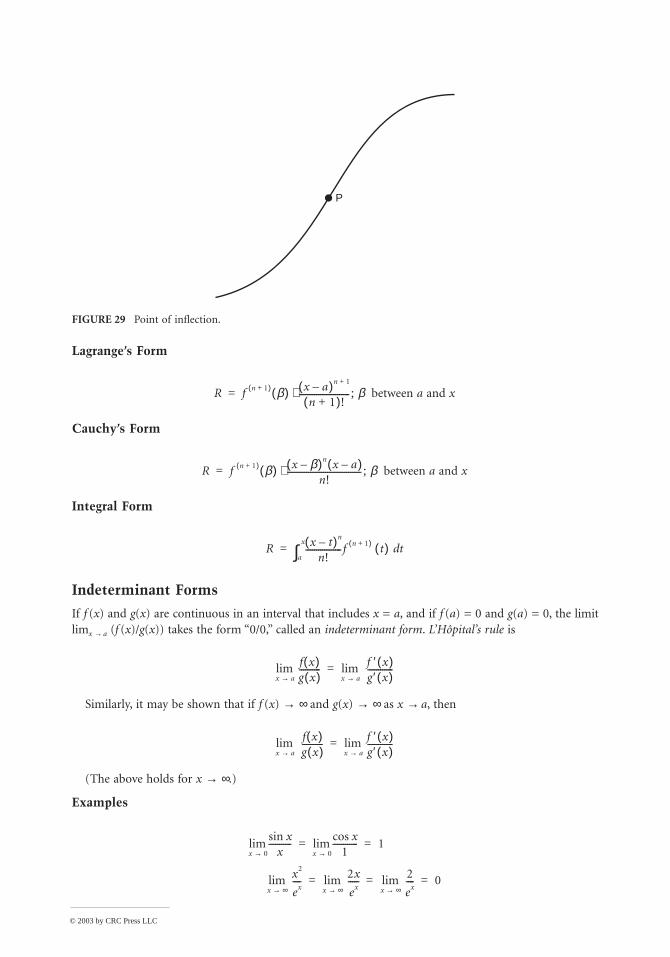
A point of the curve at which the direction of concavity changes is called a point of inflection (Figure 29). Such a point may occur where f ″(x) = 0 or where f ″(x) becomes infinite. More precisely, if the function y = f (x) and its first derivative y′ = f ′(x) are continuous in the interval a ≤ x ≤ b, and if y″ = f ″(x) exists in a < x < b, then the graph of y = f (x) for a < x < b is concave upward if f ″(x) is positive and concave downward if f ″(x) is negative.
Taylor’s Formula
If f is a function that is continuous on an interval that contains a and x, and if its first (n + 1) derivatives are continuous on this interval, then
where R is called the remainder. There are various common forms of the remainder:
R
r2 drdθ------
2
+3 2⁄
r2 2 drdθ------
2
r d2r
dθ2--------–+
---------------------------------------------=
f ″ x( ) 0>
f ″ x( ) 0<
f x( ) f a( ) f ′ a( ) x a–( ) f ″ a( )2!
------------- x a–( )2 f ″′ a( )3!
--------------- x a–( )3L
f n( ) a( )n!
--------------- x a–( )n R+ + + + + +=
© 2003 by CRC Press LLC
Lagrange’s Form
Cauchy’s Form
Integral Form
Indeterminant Forms
If f (x) and g(x) are continuous in an interval that includes x = a, and if f (a) = 0 and g(a) = 0, the limit limx → a (f (x)/g(x)) takes the form “0/0,” called an indeterminant form. L’Hôpital’s rule is
Similarly, it may be shown that if f (x) → ∞ and g(x) → ∞ as x → a, then
(The above holds for x → ∞.)
Examples
FIGURE 29 Point of inflection.
P
R f n 1+( ) β( ) x a–( )n 1+
n 1+( )!------------------------ β between a and x;⋅=
R f n 1+( ) β( ) x β–( )n x a–( )n!
----------------------------------- β between a and x;⋅=
R x t–( )n
n!-----------------f n 1+( ) t( ) td
a
x
∫=
f x( )g x( )----------
x a→lim f ′ x( )
g ′ x( )------------
x a→lim=
f x( )g x( )----------
x a→lim f ′ x( )
g ′ x( )------------
x a→lim=
xsinx
-----------x 0→lim
xcos1
------------x 0→lim 1= =
x2
ex----
x ∞→lim 2x
ex-----
x ∞→lim 2
ex----
x ∞→lim 0= = =
© 2003 by CRC Press LLC
Numerical Methods
a. Newton’s method for approximating roots of the equation f (x) = 0: A first estimate x1 of the root is made; then, provided that f ′(x1) ≠ 0, a better approximation is x2:
The process may be repeated to yield a third approximation x3 to the root:
provided f ′(x2) exists. The process may be repeated. (In certain rare cases, the process will not converge.)
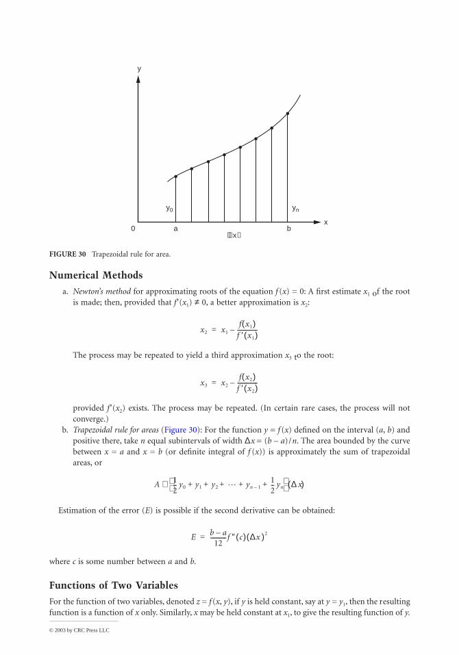
b. Trapezoidal rule for areas (Figure 30): For the function y = f (x) defined on the interval (a, b) and positive there, take n equal subintervals of width ∆x = (b – a) / n. The area bounded by the curve between x = a and x = b (or definite integral of f (x)) is approximately the sum of trapezoidal areas, or
Estimation of the error (E) is possible if the second derivative can be obtained:
where c is some number between a and b.
Functions of Two Variables
For the function of two variables, denoted z = f (x, y), if y is held constant, say at y = y1, then the resulting function is a function of x only. Similarly, x may be held constant at x1, to give the resulting function of y.
FIGURE 30 Trapezoidal rule for area.
y
y0 yn
x0 a b
∆x
x2 x1
f x1( )f ′ x1( )--------------–=
x3 x2
f x2( )f ′ x2( )--------------–=
A 12-- y0 y1 y2 L yn 1–
12-- yn+ + + + +
x∆( )∼
E b a–12
-----------f ″ c( ) x∆( )2=
© 2003 by CRC Press LLC
The Gas Laws
A familiar example is afforded by the ideal gas law that relates the pressure p, the volume V, and the absolute temperature T of an ideal gas:
where n is the number of moles and R is the gas constant per mole, 8.31 (J · K–1 · mole–1). By rearrange-ment, any one of the three variables may be expressed as a function of the other two. Further, either one of these two may be held constant. If T is held constant, then we get the form known as Boyle’s law:
(Boyle’s law)
where we have denoted nRT by the constant k and, of course, V > 0. If the pressure remains constant, we have Charles’ law:
(Charles’ law)
where the constant b denotes nR/p. Similarly, volume may be kept constant:
where now the constant, denoted a, is nR/V.
Partial Derivatives
The physical example afforded by the ideal gas law permits clear interpretations of processes in which one of the variables is held constant. More generally, we may consider a function z = f (x, y) defined over some region of the x–y-plane in which we hold one of the two coordinates, say y, constant. If the resulting function of x is differentiable at a point (x, y), we denote this derivative by one of the notations
called the partial derivative with respect to x. Similarly, if x is held constant and the resulting function of y is differentiable, we get the partial derivative with respect to y, denoted by one of the following:
Example
Integral Calculus
Indefinite Integral
If F (x) is differentiable for all values of x in the interval (a, b) and satisfies the equation dy /dx = f (x), then F (x) is an integral of f (x) with respect to x. The notation is F (x) = ∫ f (x) dx or, in differential form, dF (x) = f (x) dx.
For any function F (x) that is an integral of f (x), it follows that F (x) + C is also an integral. We thus write
pV nRT=
p kV 1–=
V bT=
p aT=
fx δf dx,⁄ δz dx⁄,
fy, δf dy⁄ δz dy⁄,
Given z x4y3 y x 4y, then+sin–=
δz dx⁄ 4 xy( )3 y xcos–=
δz dy⁄ 3x4y2 x 4+sin–=
f x( ) xd∫ F x( ) C+=
© 2003 by CRC Press LLC
Definite Integral
Let f (x) be defined on the interval [a, b] which is partitioned by points x1, x2, K, xj, K, xn – 1 between a = x0 and b = xn. The j th interval has length ∆xj = xj – xj – 1, which may vary with j. The sum where υj is arbitrarily chosen in the jth subinterval, depends on the numbers x0 , K, xn and the choice of the υ as well as f ; however, if such sums approach a common value as all ∆x approach zero, then this value is the definite integral of f over the interval (a, b) and is denoted . The fundamental theorem of integral calculus states that
where F is any continuous indefinite integral of f in the interval (a, b).
Properties
, if c is a constant
Common Applications of the Definite Integral
Area (Rectangular Coordinates)
Given the function y = f (x) such that y > 0 for all x between a and b, the area bounded by the curve y =f (x), the x-axis, and the vertical lines x = a and x = b is
Length of Arc (Rectangular Coordinates)
Given the smooth curve f (x, y) = 0 from point (x1, y1) to point (x2, y2), the length between these points is
Mean Value of a Function
The mean value of a function f (x) continuous on [a, b] is
Σj 1=n f υ j( )∆xj ,
f x( ) xda
b∫
f x( ) xda
b
∫ F b( ) F a( )–=
f1 x( ) f2 x( ) L fj x( )+ + +[ ] xda
b
∫ f1 x( ) x f2 x( ) x L fj x( ) xda
b
∫+ +da
b
∫+da
b
∫=
cf x( ) xda
b
∫ c f x( ) xda
b
∫=
f x( ) xda
b
∫ f x( ) xdb
a
∫–=
f x( ) xda
b
∫ f x( ) xda
c
∫ f x( ) xdc
b
∫+=
A f x( ) xda
b
∫=
L 1 yd xd⁄( )2+ xdx1
x2
∫=
L 1 xd yd⁄( )2+ ydy1
y2
∫=
1b a–( )
---------------- f x( ) xda
b
∫

© 2003 by CRC Press LLC
Area (Polar Coordinates)
Given the curve r = f (θ), continuous and non-negative for θ1 ≤ θ ≤ θ2, the area enclosed by this curve and the radial lines θ = θ1 and θ = θ2 is given by
Length of Arc (Polar Coordinates)
Given the curve r = f (θ) with continuous derivative f ′(θ) on θ1 ≤ θ ≤ θ2, the length of arc from θ = θ1 to θ = θ2 is
Volume of Revolution
Given a function y = f (x), continuous and non-negative on the interval (a, b), when the region bounded by f (x) between a and b is revolved about the x-axis, the volume of revolution is
Surface Area of Revolution (Revolution about the x-axis, between a and b)
If the portion of the curve y = f (x) between x = a and x = b is revolved about the x-axis, the area A of the surface generated is given by the following:
Work
If a variable force f (x) is applied to an object in the direction of motion along the x-axis between x = aand x = b, the work done is
Cylindrical and Spherical Coordinates
a. Cylindrical coordinates (Figure 31)
element of volume dV = r dr dθ dz.b. Spherical coordinates (Figure 32)
element of volume dV = ρ2 sin φ dρ, dφ dθ.
A 12-- f θ( )[ ] 2 θd
θ1
θ2
∫=
L f θ( )[ ] 2 f ′ θ( )[ ] 2+ θdθ1
θ2∫=
V π f x( )[ ] 2 xda
b
∫=
A 2πf x( ) 1 f ′ x( )[ ] 2+ 1 2⁄xd
a
b
∫=
W f x( ) xda
b
∫=
x r θcos=
y r θsin=
x ρ φ θcossin=
y ρ φ θsinsin=
z ρ φcos=
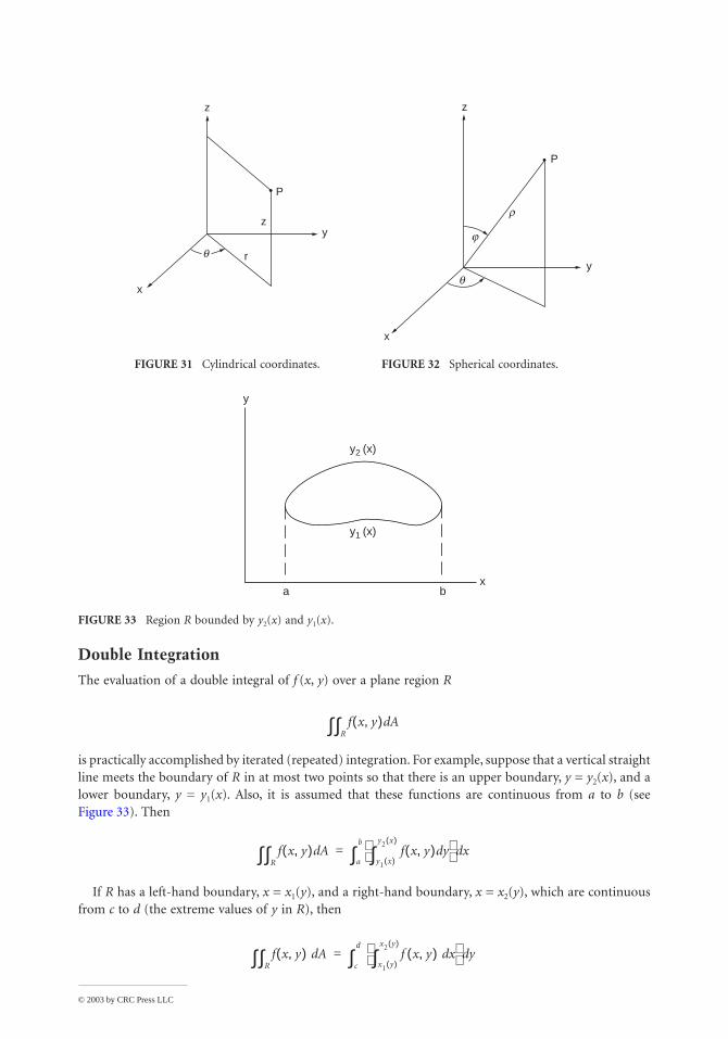
© 2003 by CRC Press LLC
Double Integration
The evaluation of a double integral of f (x, y) over a plane region R
is practically accomplished by iterated (repeated) integration. For example, suppose that a vertical straight line meets the boundary of R in at most two points so that there is an upper boundary, y = y2(x), and a lower boundary, y = y1(x). Also, it is assumed that these functions are continuous from a to b (see Figure 33). Then
If R has a left-hand boundary, x = x1(y), and a right-hand boundary, x = x2(y), which are continuous from c to d (the extreme values of y in R), then
FIGURE 31 Cylindrical coordinates. FIGURE 32 Spherical coordinates.
FIGURE 33 Region R bounded by y2(x) and y1(x).
z
P
z
r
y
x
q
r
q
j
y
z
P
x
y2 (x)
y1 (x)
xba
y
f x y,( ) AdR∫∫
f x y,( ) AdR∫∫ f x y,( ) yd
y1 x( )
y2 x( )
∫ xd
a
b
∫=
f x y,( ) AdR∫∫ f x y,( ) xd
x1 y( )
x2 y( )
∫ yd
c
d
∫=
© 2003 by CRC Press LLC
Such integrations are sometimes more convenient in polar coordinates, x = r cos θ, y = r sin θ; dA = r dr dθ.
Surface Area and Volume by Double Integration
For the surface given by z = f (x, y), which projects onto the closed region R of the x–y-plane, one may calculate the volume V bounded above by the surface and below by R, and the surface area S by the following:
[In polar coordinates (r, θ ), we replace dA by r dr dθ ].
Centroid
The centroid of a region R of the x–y-plane is a point (x′, y′) where
and A is the area of the region.
Example.
For the circular sector of angle 2α and radius R, the area A is α R2; the integral needed for x ′, expressed in polar coordinates, is
Thus,
Centroids of some common regions are shown in Figure 34.
Vector Analysis
Vectors
Given the set of mutually perpendicular unit vectors i, j, and k (Figure 35), any vector in the space may be represented as F = ai + bj + ck, where a, b, and c are components.
Magnitude of F
V z AdR∫∫ f x y,( ) xd yd
R∫∫= =
S 1 δz δx⁄( )2 δz δy⁄( )2+ +[ ] 1 2⁄xd yd
R∫∫=
x ′ 1A--- x A y ′ 1
A - - - y A d
R ∫ ∫ = d
R ∫ ∫ =
x Ad∫∫ r θcos( )r rd θd0
R
∫α–
α
∫=
R3
3----- θsin
α–
α+ 23--R3 αsin= =
x ′
23--R3 αsin
αR2--------------------- 2
3--R αsin
α-----------= =
F a2 b2 c2+ +( )12--
=
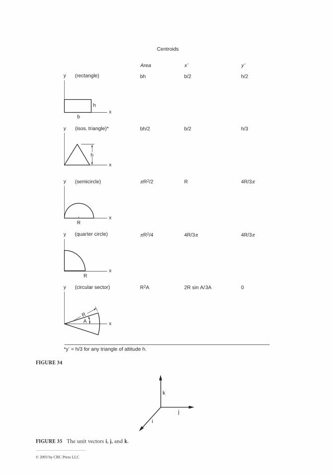
© 2003 by CRC Press LLC
FIGURE 34
FIGURE 35 The unit vectors i, j, and k.
y
x
y
x
y
x
y
x
y
x
(rectangle)
h
h
b
(isos. triangle)*
(semicircle)
R
(quarter circle)
R
(circular sector)
*y′ = h/3 for any triangle of altitude h.
RA
Area x ′ y ′
bh b/2 h/2
bh/2 b/2 h/3
pR2/2 R 4R/3p
pR2/4 4R/3p 4R/3p
R2A 2R sin A/3A 0
Centroids
k
j
i
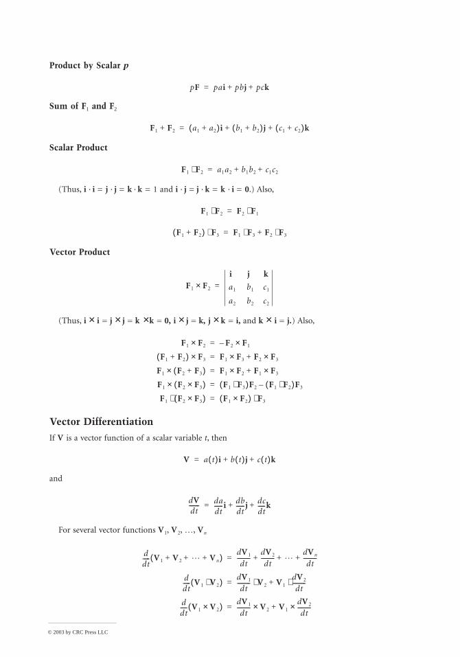
© 2003 by CRC Press LLC
Product by Scalar p
Sum of F1 and F2
Scalar Product
(Thus, i · i = j · j = k · k = 1 and i · j = j · k = k · i = 0.) Also,
Vector Product
(Thus, i × i = j × j = k × k = 0, i × j = k, j × k = i, and k × i = j.) Also,
Vector Differentiation
If V is a vector function of a scalar variable t, then
and
For several vector functions V1, V2, K, Vn
pF pai pbj pck+ +=
F1 F2+ a1 a2+( )i b1 b2+( )j c1 c2+( )k+ +=
F1 F2⋅ a1a2 b1b2 c1c2+ +=
F1 F2⋅ F2 F1⋅=
F1 F2+( ) F3⋅ F1 F3 F2 F3⋅+⋅=
F1 F2×i j k
a1 b1 c1
a2 b2 c2
=
F1 F2× F2 F1×–=
F1 F2+( ) F3× F1 F3 F2 F3×+×=
F1 F2 F3+( )× F1 F2 F1 F3×+×=
F1 F2 F3×( )× F1 F3⋅( )F2 F1 F2⋅( )F3–=
F1 F2 F3×( )⋅ F1 F2×( ) F3⋅=
V a t( )i b t( )j c t( )k+ +=
dVdt------- da
dt------i db
dt------j dc
dt-----k+ +=
ddt----- V1 V2 L Vn+ + +( )
dV1
dt---------
dV2
dt--------- L
dVn
dt---------+ + +=
ddt----- V1 V2⋅( ) dV1
dt--------- V2 V1
dV2
dt---------⋅+⋅=
ddt----- V1 V2×( ) dV1
dt--------- V2 V1
dV2
dt---------×+×=
© 2003 by CRC Press LLC
For a scalar-valued function g(x, y, z)
For a vector-valued function V(a, b, c), where a, b, and c are each a function of x, y, and z,
(divergence)
(curl)
Also,
and
Divergence Theorem (Gauss)
Given a vector function F with continuous partial derivatives in a region R bounded by a closed surface S, then
where n is the (sectionally continuous) unit normal to S.
Stokes’ Theorem
Given a vector function with continuous gradient over a surface S that consists of portions that are piecewise smooth and bounded by regular closed curves such as C,
Planar Motion in Polar Coordinates
Motion in a plane may be expressed with regard to polar coordinates (r, θ ). Denoting the position vector by r and its magnitude by r, we have r = rR(θ ), where R is the unit vector. Also, dR/dθ = P, a unit vector perpendicular to R. The velocity and acceleration are then
gradient( ) grad g ∇ g δgδx------i δg
δy------j δg
δ z------k+ += =
divV ∇ V⋅ δaδx------
δbδy------
δ cδ z------+ += =
curlV ∇ V×
i j k
δδx------ δ
δy------ δ
δ z------
a b c
= =
div grad g ∇ 2gδ 2g
δx2--------
δ 2g
δy2-------
δ 2g
δz2-------+ += =
curl grad g 0; div curl V 0;= =
curl curlV grad divV i ∇ 2a j∇ 2b k ∇ 2c+ +( )–=
iv F⋅d VdR∫∫∫ n F Sd⋅
S∫∫=
n curl F⋅ SdS∫∫ F dr⋅
C∫°=
v drdt-----R rdθ
dt------P+=
a d2rdt2------- r dθ
dt------
2
– R rd2θdt2-------- 2dr
dt-----
dθdt------+ P+=
© 2003 by CRC Press LLC
Note that the component of acceleration in the P direction (transverse component) may also be written
so that in purely radial motion it is zero and
which means that the position vector sweeps out area at a constant rate [see Area (Polar Coordinates) in the section entitled Integral Calculus].
Special Functions
Hyperbolic Functions
Laplace Transforms
The Laplace transform of the function f (t), denoted by F (s) or Lf (t), is defined
1r--
ddt----- r2dθ
dt------
r2dθdt------ C cons ttan( )=
xsinhex e x––
2----------------= xcsch
1 xsinh
---------------=
xcoshex e x–+
2-----------------= xsech
1xcosh
----------------=
xtanhex e x––ex e x–+-----------------= ctnh x
1xtanh
----------------=
x–( )sinh xsinh–= ctnh x–( ) ctnh x–=
x–( )cosh xcosh= x–( )sech xsech=
x–( )tanh xtanh–= hcsc x–( ) xcsch–=
xtanhxsinhxcosh
----------------= ctnh xxcoshxsinh
----------------=
h2 x h2 xsin–cos 1= h2 xcos 12-- 2x 1+cosh( )=
h2sin x 12-- 2x 1–cosh( )= ctnh2 x csch2 x– 1=
h2 x sech2 x–csc h2csc x h2 xsec= h2tan x sech2 x+ 1=
h x y+( )sin x y x ysinhcosh+coshsinh=
x y+( )cosh x y x ysinhsinh+coshcosh=
h x y–( )sin x y x ysinhcosh–coshsinh=
x y–( )cosh x y x ysinhsinh–coshcosh=
x y+( )tanhx ytanh+tanh
1 x ytanhtanh+-------------------------------------------=
x y–( )tanhx ytanh–tanh
1 x ytanhtanh–------------------------------------------=
F s( ) f t( )e st– td0
∞
∫=
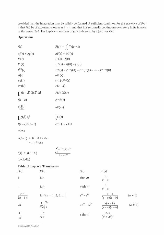
© 2003 by CRC Press LLC
provided that the integration may be validly performed. A sufficient condition for the existence of F (s) is that f (t) be of exponential order as t → ∞ and that it is sectionally continuous over every finite interval in the range t ≥ 0. The Laplace transform of g(t) is denoted by Lg(t) or G(s).
Operations
where
(periodic)
Table of Laplace Transforms
f (t) F (s) f (t) F (s)
1 1/s
t 1/s2
1/sn (n = 1, 2, 3, K) (a ≠ b)
(a ≠ b)
f t( ) F s( ) f t( )e st– td0
∞
∫=
af t( ) bg t( )+ aF s( ) bG s( )+
f ′ t( ) sF s( ) f 0( )–
f ″ t( ) s2F s( ) sf 0( )– f ′ 0( )–
f n( ) t( ) snF s( ) sn 1– f 0( )– sn 2– f ′ 0( )– L– f n 1–( ) 0( )–
tf t( ) F ′ s( )–
tnf t( ) 1–( )nF n( ) s( )
eatf t( ) F s a–( )
f t β–( ) g β( )⋅ βd0
t
∫ F s( ) G s( )⋅
f t a–( ) e as– F s( )
f ta--
aF as( )
g β( ) βd0
t
∫ 1s--G s( )
f t c–( )δ t c–( ) e cs– F s( ) c 0>,
δ t c–( ) 0 if 0 t c<≤=
1 if t c≥=
f t( ) f t ω+( )=e sτ– f τ( ) τd
0
ω
∫1 e sω––
-----------------------------
h asin t as2 a2–--------------
atcosh ss2 a2–--------------
tn 1–
n 1–( )!------------------ eat ebt– a b–
s a–( ) s b–( )-------------------------------
t 12s-----
πs--- aeat bebt– s a b–( )
s a–( ) s b–( )-------------------------------
1
t-----
πs--- t asin t 2as
s2 a2+( )2----------------------
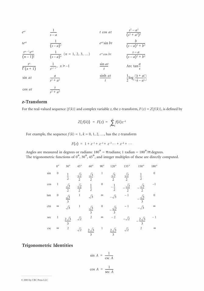
© 2003 by CRC Press LLC
eat
teat
(n = 1, 2, 3, K)
z-Transform
For the real-valued sequence f (k) and complex variable z, the z-transform, F (z) = Zf (k), is defined by
For example, the sequence f (k) = 1, k = 0, 1, 2, K, has the z-transform
Angles are measured in degrees or radians: 180° = π radians; 1 radian = 180°/π degrees. The trigonometric functions of 0°, 30°, 45°, and integer multiples of these are directly computed.
Trigonometric Identities
0° 30° 45° 60° 90° 120° 135° 150° 180°
sin 0 1 0
cos 1 0 –1
tan 0 1 ∞ – 1 0
ctn ∞ 1 0 – 1 ∞
sec 1 2 ∞ – 2 – 1
csc ∞ 2 1 2 ∞
1s a–---------- t atcos s2 a2–
s2 a2+( )2----------------------
1s a–( )2
----------------- eat btsin bs a–( )2 b2+
-----------------------------
tn 1– eat
n 1–( )!------------------
1s a–( )n
----------------- eat btcoss a–
s a–( )2 b2+-----------------------------
tx
Γ x 1+( )---------------------
1sx 1+--------- , x 1–> atsin
t------------- Arc
as--tan
atsin as2 a2+---------------
asinh tt
-----------------12--
s a+s a–-----------
e
log
acos t ss2 a2+---------------
Z f k( ) F z( ) f k( )z k–
k 0=
∞
∑= =
F z( ) 1 z 1– z 2– z 3– L z k– L+ + + + +=
12-- 2
2------- 3
2------- 3
2------- 2
2-------
12--
32
------- 22
-------12-- 1
2--– 2
2-------– 3
2-------–
33
-------3 3– 3
3-------–
3 33
------- 33
-------– 3–
2 33
----------2 2– 2 3
3----------–
2 2 33
---------- 2 33
----------2
Asin1
Acsc-------------=
Acos1
Asec-------------=
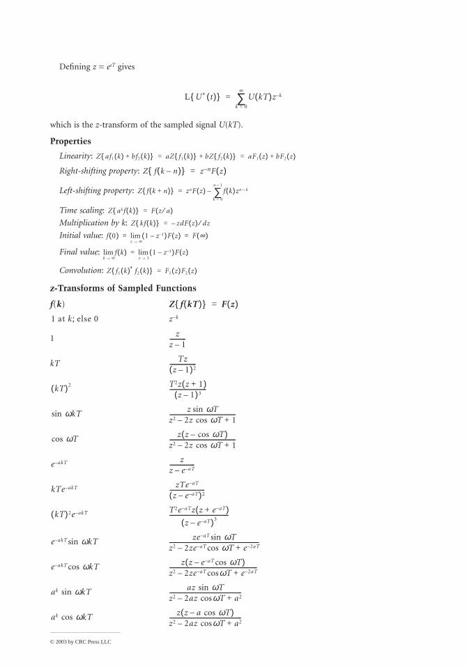
© 2003 by CRC Press LLC
Defining z = esT gives
which is the z-transform of the sampled signal U(kT).
Properties
Linearity:
Right-shifting property:
Left-shifting property:
Time scaling:
Multiplication by k:
Initial value:
Final value:
Convolution:
z-Transforms of Sampled Functions
f(k)
1
kT
L U* t( ) U kT( )z k–
k 0=
∞
∑=
Z af1 k( ) bf2 k( )+ aZ f1 k( ) bZ f2 k( ) + aF1 z( ) bF2 z( )+= =
Z f k n–( ) z n– F z( )=
Z f k n+( ) znF z( ) f k( )zn k–
k 0=
n 1–
∑–=
Z akf k( ) F z a⁄( )=
Z kf k( ) zdF z( ) dz⁄–=
f 0( ) 1 z 1––( )F z( )z ∞→lim F ∞( )= =
f k( )k ∞→lim 1 z 1––( )
z 1→lim F z( )=
Z f1 k( )* f2 k( ) F1 z( )F2 z( )=
Z f kT( ) F z( )=
1 at k else 0; z k–
zz 1–-----------
Tzz 1–( )2
------------------
kT( )2 T2z z 1+( )z 1–( )3
-------------------------
ωkTsin z ωTsinz2 2z ωT 1+cos–---------------------------------------------
ωTcos z z ωTcos–( )z2 2z ωT 1+cos–---------------------------------------------
e akT– zz e aT––-----------------
kTe akT– zTe aT–
z e a– T–( )2------------------------
kT( )2e akT– T2e aT– z z e aT–+( )z e aT––( )3
----------------------------------------
e akT– ωkTsin ze aT– ωTsinz2 2ze aT– ωT e 2aT–+cos–-------------------------------------------------------------
e akT– ωcos kT z z e– aT– ωcos T( )z2 2ze aT– ωT e 2aT–+cos–------------------------------------------------------------
ak ωsin kT az ωsin Tz2 2az ωT a2+cos–-------------------------------------------------
ak ωcos kT z z a– ωcos T( )z2 2az ωT a2+cos–-------------------------------------------------
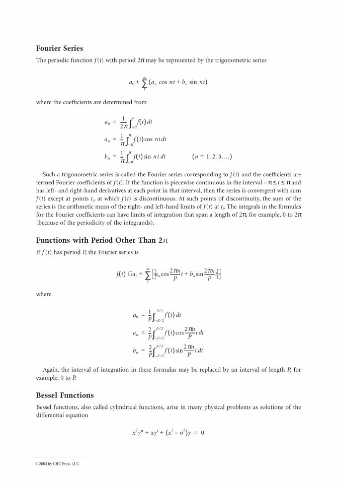
© 2003 by CRC Press LLC
Fourier Series
The periodic function f (t) with period 2π may be represented by the trigonometric series
where the coefficients are determined from
Such a trigonometric series is called the Fourier series corresponding to f (t) and the coefficients are termed Fourier coefficients of f (t). If the function is piecewise continuous in the interval – π ≤ t ≤ π and has left- and right-hand derivatives at each point in that interval, then the series is convergent with sum f (t) except at points ti , at which f (t) is discontinuous. At such points of discontinuity, the sum of the series is the arithmetic mean of the right- and left-hand limits of f (t) at ti. The integrals in the formulas for the Fourier coefficients can have limits of integration that span a length of 2π, for example, 0 to 2π(because of the periodicity of the integrands).
Functions with Period Other Than 2πIf f (t) has period P, the Fourier series is
where
Again, the interval of integration in these formulas may be replaced by an interval of length P, for example, 0 to P.
Bessel Functions
Bessel functions, also called cylindrical functions, arise in many physical problems as solutions of the differential equation
a0 an nt bn ntsin+cos( )1
∞
∑+
a01
2π------ f t( ) tdπ–
π
∫=
an1π---
f t( ) nt tdcosπ–
π
∫=
bn1π---
f t( ) nsin t t dπ–
π
∫ n 1, 2, 3,K=( )=
f t( ) a0 an2πn
P----------t bn
2πnP
----------tsin+cos
1
∞
∑+∼
a01P--- f t( ) td
P 2⁄–
P 2⁄
∫=
an2P--- f t( ) 2πn
P----------cos t td
P 2⁄–
P 2⁄
∫=
bn2P--- f t( ) 2πn
P----------sin t td
P 2⁄–
P 2⁄
∫=
x2y″ xy ′ x2 n2–( )y+ + 0=
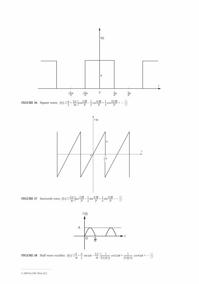
© 2003 by CRC Press LLC
FIGURE 36 Square wave.
FIGURE 37 Sawtooth wave. .
FIGURE 38 Half-wave rectifier.
f(t)
a
t
−12P −1
4P 14P 1
2P0
f t( ) a2--- 2a
π------ 2πt
P--------- 1
3--- 6πt
P--------- 1
3--- 10πt
P------------ L +cos+cos–cos
.+∼
f (t)
a
o
t
P12
f t( ) 2aπ
------ 2πtP
--------- 12--- 4πt
P--------- 1
3--- 6πt
P--------- L –sin+sin–sin
∼
f (t)
A
Otπ
ω
f t( ) Aπ--- A
2--- ωt 2A
π------- 1
1( ) 3( )---------------- 2ωt 1
3( ) 5( )---------------- 4ωt L +cos+cos
.–sin+∼
© 2003 by CRC Press LLC
which is known as Bessel’s equation. Certain solutions of the above, known as Bessel functions of the first kind of order n, are given by
In the above it is noteworthy that the gamma function must be defined for the negative argument q: Γ(q) = Γ(q + 1)/q, provided that q is not a negative integer. When q is a negative integer, 1/Γ(q) is defined to be zero. The functions J–n (x) and Jn (x) are solutions of Bessel’s equation for all real n. It is seen, for n = 1, 2, 3, K, that
and, therefore, these are not independent; hence, a linear combination of these is not a general solution. When, however, n is not a positive integer, a negative integer, or zero, the linear combination with arbitrary constants c1 and c2
is the general solution of the Bessel differential equation.The zero-order function is especially important as it arises in the solution of the heat equation (for a
“long” cylinder):
while the following relations show a connection to the trigonometric functions:
The following recursion formula gives Jn + 1(x) for any order in terms of lower-order functions:
Legendre Polynomials
If Laplace’s equation, ∇ 2V = 0, is expressed in spherical coordinates, it is
and any of its solutions, V (r, θ, φ), are known as spherical harmonics. The solution as a product
Jn x( ) 1–( )k
k!Γ n k 1+ +( )-----------------------------------
x2--
n 2k+
k 0=
∞
∑=
J n– x( ) 1–( )k
k!Γ n– k 1+ +( )----------------------------------------
x2--
n– 2k+
k 0=
∞
∑=
J n– x( ) 1–( )nJn x( )=
y c1Jn x( ) c2J n– x( )+=
J0 x( ) 1x2
22----–
x4
2242----------
x6
224262---------------– L+ +=
J12--
x( ) 2πx------
1 2⁄
xsin=
J 12--–
x( ) 2πx------
1 2⁄
xcos=
2nx
------Jn x( ) Jn 1– x( ) Jn 1+ x( )+=
r2 θ δ2V
δr2---------sin 2r θ δV
δr-------sin θ δ2V
δθ2---------sin θcos δV
δθ-------1
θsin-----------
δ2V
δφ2---------+ + + + 0=
© 2003 by CRC Press LLC
which is independent of φ, leads to
Rearrangement and substitution of x = cosθ leads to
known as Legendre’s equation. Important special cases are those in which n is zero or a positive integer, and, for such cases, Legendre’s equation is satisfied by polynomials called Legendre polynomials, Pn(x). A short list of Legendre polynomials, expressed in terms of x and cos θ, is given below. These are given by the following general formula:
where L = n/2 if n is even and L = (n – 1)/2 if n is odd.
Additional Legendre polynomials may be determined from the recursion formula
or the Rodrigues formula
V r θ φ, ,( ) R r( ) Θ θ( )=
θ2sin Θ″ θ θΘ′cossin n n 1+( ) θ2
sin[ ]Θ+ + 0=
1 x2–( )x2
2
d
d Θ 2xxd
dΘ– n n 1+( )Θ+ 0=
Pn x( ) 1–( ) j 2n 2j–( )!2nj! n j–( )! n 2j–( )!-----------------------------------------------xn 2 j–
j 0=
L
∑=
P0 x( ) 1=
P1 x( ) x=
P2 x( ) 12-- 3x2 1–( )=
P3 x( ) 12-- 5x3 3x–( )=
P4 x( ) 18-- 35x4 30x2– 3+( )=
P5 x( ) 18-- 63x5 70x3– 15x+( )=
P0 θcos( ) 1=
P1 θcos( ) θcos=
P2 θcos( ) 14-- 3 2θ 1+cos( )=
P3 θcos( ) 18-- 5 3θ 3 θcos+cos( )=
P4 θcos( ) 164----- 35 4θ 20 2θ 9+cos+cos( )=
n 1+( )Pn 1+ x( ) 2n 1+( )xPn x( ) nPn 1– x( )+– 0 (n 1, 2, K )= =
Pn x( ) 1
2nn!----------
dn
dxn-------- x2 1–( )n
=
© 2003 by CRC Press LLC
Laguerre Polynomials
Laguerre polynomials, denoted Ln (x), are solutions of the differential equation
and are given by
Thus,
Additional Laguerre polynomials may be obtained from the recursion formula
Hermite Polynomials
The Hermite polynomials, denoted Hn (x), are given by
and are solutions of the differential equation
The first few Hermite polynomials are
Additional Hermite polynomials may be obtained from the relation
where prime denotes differentiation with respect to x.
Orthogonality
A set of functions fn (x) (n = 1, 2, K ) is orthogonal in an interval (a, b) with respect to a given weight function w(x) if
xy ″ 1 x–( )y ′ ny+ + 0=
Ln x( ) 1–( ) j
j!------------
j 0=
n
∑ C n j,( )xj (n 0, 1, 2, K )==
L0 x( ) 1=
L1 x( ) 1 x–=
L2 x( ) 1 2x– 12--x2+=
L3 x( ) 1 3x– 32--x2 1
6--x3–+=
n 1+( )Ln 1+ x( ) 2n 1 x–+( )Ln x( )– nLn 1– x( )+ 0=
H0 1= Hn x( ), 1–( )nex2 dne x
2–
dxn------------- (n 1, 2, K )==
y″ 2xy ′– 2ny+ 0 (n 0, 1, 2, K )==
H0 1 H1 x( ) 2x= =
H2 x( ) 4x2 2 H3 x( )– 8x2 12x–= =
H4 x( ) 16x4 48x2– 12+=
Hn 1+ x( ) 2xHn x( ) H ′n x( )–=
w x( ) fm x( ) fn x( ) xda
b
∫ 0 when m n≠=
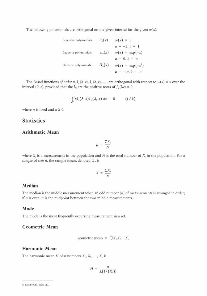
© 2003 by CRC Press LLC
The following polynomials are orthogonal on the given interval for the given w(x):
The Bessel functions of order n, Jn (λ1x), Jn (λ2x), K, are orthogonal with respect to w(x) = x over the interval (0, c), provided that the λi are the positive roots of Jn (λc) = 0:
where n is fixed and n ≥ 0.
Statistics
Arithmetic Mean
where Xi is a measurement in the population and N is the total number of Xi in the population. For a sample of size n, the sample mean, denoted , is
Median
The median is the middle measurement when an odd number (n) of measurements is arranged in order; if n is even, it is the midpoint between the two middle measurements.
Mode
The mode is the most frequently occurring measurement in a set.
Geometric Mean
Harmonic Mean
The harmonic mean H of n numbers X1, X2, K, Xn is
Legendre polynomials:
Laguerre polynomials:
Hermite polynomials
Pn x( ) w x( ) 1=
a 1, b– 1= =
Ln x( ) w x( ) x–( )exp=
a 0, b ∞= =
Hn x( ) w x( ) x2–( )exp=
a ∞– b, ∞= =
xJn λ j x( )J n λ k x( ) xd0
c
∫ 0 j k≠( )=
µ ΣXi
N--------=
X
XΣXi
n--------=
geometric mean X1X2KXn
n=
Hn
Σ 1 Xi( )⁄( )--------------------------=
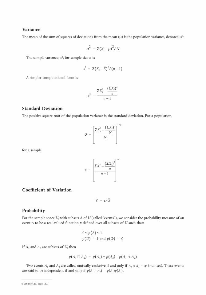
© 2003 by CRC Press LLC
Variance
The mean of the sum of squares of deviations from the mean (µ) is the population variance, denoted σ2:
The sample variance, s 2, for sample size n is
A simpler computational form is
Standard Deviation
The positive square root of the population variance is the standard deviation. For a population,
for a sample
Coefficient of Variation
Probability
For the sample space U, with subsets A of U (called “events”), we consider the probability measure of an event A to be a real-valued function p defined over all subsets of U such that:
If A1 and A2 are subsets of U, then
Two events A1 and A2 are called mutually exclusive if and only if (null set). These events are said to be independent if and only if
σ2 Σ Xi µ–( )2N⁄=
s2 Σ Xi X–( )2n 1–( )⁄=
s2ΣXi
2 ΣXi( )2
n---------------–
n 1–-------------------------------=
σΣXi
2 ΣXi( )2
N---------------–
N-------------------------------
1 2⁄
=
sΣXi
2 ΣXi( )2
n---------------–
n 1–-------------------------------
1 2⁄
=
V s X⁄=
0 p A( ) 1≤≤p U( ) 1 and p Φ( ) 0= =
p A1 A2∪( ) p A1( ) p A2( ) p A1 A2∩( )–+=
A1 A2∩ φ=
p A1 A2∩( ) p A1( )p A2( ) .=
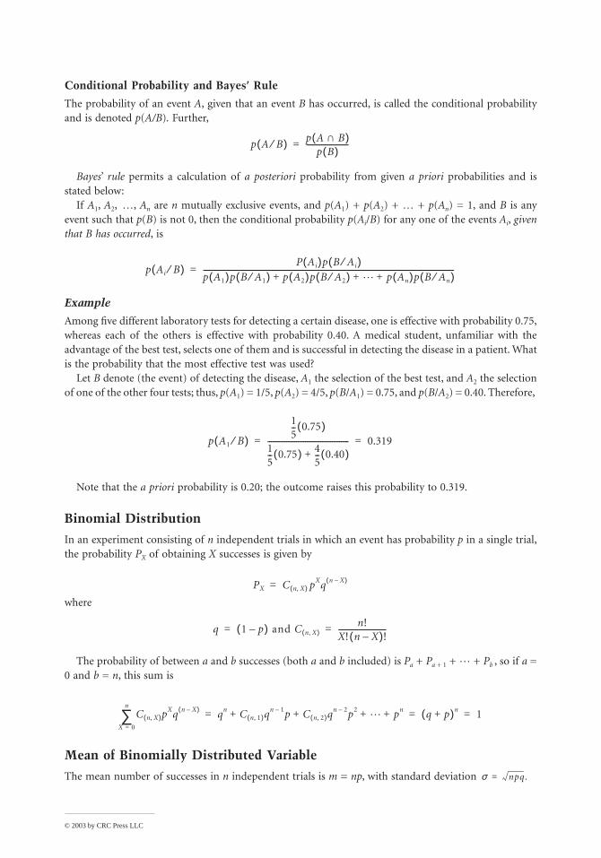
© 2003 by CRC Press LLC
Conditional Probability and Bayes’ Rule
The probability of an event A, given that an event B has occurred, is called the conditional probability and is denoted p(A/B). Further,
Bayes’ rule permits a calculation of a posteriori probability from given a priori probabilities and is stated below:
If A1, A2, K, An are n mutually exclusive events, and p(A1) + p(A2) + K + p(An) = 1, and B is any event such that p(B) is not 0, then the conditional probability p(Ai/B) for any one of the events Ai, giventhat B has occurred, is
Example
Among five different laboratory tests for detecting a certain disease, one is effective with probability 0.75, whereas each of the others is effective with probability 0.40. A medical student, unfamiliar with the advantage of the best test, selects one of them and is successful in detecting the disease in a patient. What is the probability that the most effective test was used?
Let B denote (the event) of detecting the disease, A1 the selection of the best test, and A2 the selection of one of the other four tests; thus, p(A1) = 1/5, p(A2) = 4/5, p(B/A1) = 0.75, and p(B/A2) = 0.40. Therefore,
Note that the a priori probability is 0.20; the outcome raises this probability to 0.319.
Binomial Distribution
In an experiment consisting of n independent trials in which an event has probability p in a single trial, the probability PX of obtaining X successes is given by
where
The probability of between a and b successes (both a and b included) is Pa + Pa + 1 + L + Pb , so if a = 0 and b = n, this sum is
Mean of Binomially Distributed Variable
The mean number of successes in n independent trials is m = np, with standard deviation
p A B⁄( ) p A B∩( )p B( )
----------------------=
p Ai B⁄( )P Ai( )p B Ai⁄( )
p A1( )p B A1⁄( ) p A2( )p B A2⁄( ) L p An( )p B An⁄( )+ + +-------------------------------------------------------------------------------------------------------------------------------------=
p A1 B⁄( )
15-- 0.75( )
15-- 0.75( ) 4
5-- 0.40( )+
------------------------------------------- 0.319= =
PX C n X,( ) pXq n X–( )=
q 1 p–( ) and C n X,( )n!
X! n X–( )!-------------------------= =
C n X,( )pXq n X–( )
X 0=
n
∑ qn C n 1,( )qn 1– p C n 2,( )q
n 2– p2L pn+ + + + q p+( )n 1= = =
σ npq .=
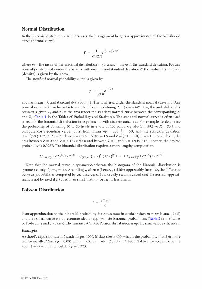
© 2003 by CRC Press LLC
Normal Distribution
In the binomial distribution, as n increases, the histogram of heights is approximated by the bell-shaped curve (normal curve)
where m = the mean of the binomial distribution = np, and is the standard deviation. For any normally distributed random variable X with mean m and standard deviation σ, the probability function (density) is given by the above.
The standard normal probability curve is given by
and has mean = 0 and standard deviation = 1. The total area under the standard normal curve is 1. Any normal variable X can be put into standard form by defining Z = (X – m)/σ; thus, the probability of Xbetween a given X1 and X2 is the area under the standard normal curve between the corresponding Z1
and Z2 (Table 1 in the Tables of Probability and Statistics). The standard normal curve is often used instead of the binomial distribution in experiments with discrete outcomes. For example, to determine the probability of obtaining 60 to 70 heads in a toss of 100 coins, we take X = 59.5 to X = 70.5 and compute corresponding values of Z from mean np = 100 = 50, and the standard deviation
Thus, Z = (59.5 – 50)/5 = 1.9 and Z = (70.5 – 50)/5 = 4.1. From Table 1, the area between Z = 0 and Z = 4.1 is 0.5000 and between Z = 0 and Z = 1.9 is 0.4713; hence, the desired probability is 0.0287. The binomial distribution requires a more lengthy computation.
Note that the normal curve is symmetric, whereas the histogram of the binomial distribution is symmetric only if p = q = 1/2. Accordingly, when p (hence, q) differs appreciably from 1/2, the difference between probabilities computed by each increases. It is usually recommended that the normal approxi-mation not be used if p (or q) is so small that np (or nq) is less than 5.
Poisson Distribution
is an approximation to the binomial probability for r successes in n trials when m = np is small (< 5) and the normal curve is not recommended to approximate binomial probabilities (Table 2 in the Tables of Probability and Statistics). The variance σ 2 in the Poisson distribution is np, the same value as the mean.
Example
A school’s expulsion rate is 5 students per 1000. If class size is 400, what is the probability that 3 or more will be expelled? Since p = 0.005 and n = 400, m = np = 2 and r = 3. From Table 2 we obtain for m = 2 and r ( = x) = 3 the probability p = 0.323.
Y 1
σ 2π-------------- e x m–( )2
2σ2⁄–=
σ npq=
y 1
2π---------- e Z–
22⁄=
12--
σ 100( ) 1 2⁄( ) 1 2⁄( ) 5.= =
C 100 60,( ) 1 2⁄( )60 1 2⁄( )40 C 100 61,( ) 1 2⁄( )61 1 2⁄( )39L C 100 70,( ) 1 2⁄( )70 1 2⁄( )30+ + +
Pe m– m
r
r!--------------=
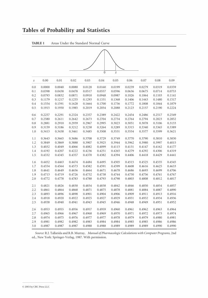
© 2003 by CRC Press LLC
Tables of Probability and Statistics
TABLE 1 Areas Under the Standard Normal Curve
z 0.00 0.01 0.02 0.03 0.04 0.05 0.06 0.07 0.08 0.09
0.0 0.0000 0.0040 0.0080 0.0120 0.0160 0.0199 0.0239 0.0279 0.0319 0.03590.1 0.0398 0.0438 0.0478 0.0517 0.0557 0.0596 0.0636 0.0675 0.0714 0.07530.2 0.0793 0.0832 0.0871 0.0910 0.0948 0.0987 0.1026 0.1064 0.1103 0.11410.3 0.1179 0.1217 0.1255 0.1293 0.1331 0.1368 0.1406 0.1443 0.1480 0.15170.4 0.1554 0.1591 0.1628 0.1664 0.1700 0.1736 0.1772 0.1808 0.1844 0.18790.5 0.1915 0.1950 0.1985 0.2019 0.2054 0.2088 0.2123 0.2157 0.2190 0.2224
0.6 0.2257 0.2291 0.2324 0.2357 0.2389 0.2422 0.2454 0.2486 0.2517 0.25490.7 0.2580 0.2611 0.2642 0.2673 0.2704 0.2734 0.2764 0.2794 0.2823 0.28520.8 0.2881 0.2910 0.2939 0.2967 0.2995 0.3023 0.3051 0.3078 0.3106 0.31330.9 0.3159 0.3186 0.3212 0.3238 0.3264 0.3289 0.3315 0.3340 0.3365 0.33891.0 0.3413 0.3438 0.3461 0.3485 0.3508 0.3531 0.3554 0.3577 0.3599 0.3621
1.1 0.3643 0.3665 0.3686 0.3708 0.3729 0.3749 0.3770 0.3790 0.3810 0.38301.2 0.3849 0.3869 0.3888 0.3907 0.3925 0.3944 0.3962 0.3980 0.3997 0.40151.3 0.4032 0.4049 0.4066 0.4082 0.4099 0.4115 0.4131 0.4147 0.4162 0.41771.4 0.4192 0.4207 0.4222 0.4236 0.4251 0.4265 0.4279 0.4292 0.4306 0.43191.5 0.4332 0.4345 0.4357 0.4370 0.4382 0.4394 0.4406 0.4418 0.4429 0.4441
1.6 0.4452 0.4463 0.4474 0.4484 0.4495 0.4505 0.4515 0.4525 0.4535 0.45451.7 0.4554 0.4564 0.4573 0.4582 0.4591 0.4599 0.4608 0.4616 0.4625 0.46331.8 0.4641 0.4649 0.4656 0.4664 0.4671 0.4678 0.4686 0.4693 0.4699 0.47061.9 0.4713 0.4719 0.4726 0.4732 0.4738 0.4744 0.4750 0.4756 0.4761 0.47672.0 0.4772 0.4778 0.4783 0.4788 0.4793 0.4798 0.4803 0.4808 0.4812 0.4817
2.1 0.4821 0.4826 0.4830 0.4834 0.4838 0.4842 0.4846 0.4850 0.4854 0.48572.2 0.4861 0.4864 0.4868 0.4871 0.4875 0.4878 0.4881 0.4884 0.4887 0.48902.3 0.4893 0.4896 0.4898 0.4901 0.4904 0.4906 0.4909 0.4911 0.4913 0.49162.4 0.4918 0.4920 0.4922 0.4925 0.4927 0.4929 0.4931 0.4932 0.4934 0.49362.5 0.4938 0.4940 0.4941 0.4943 0.4945 0.4946 0.4948 0.4949 0.4951 0.4952
2.6 0.4953 0.4955 0.4956 0.4957 0.4959 0.4960 0.4961 0.4962 0.4963 0.49642.7 0.4965 0.4966 0.4967 0.4968 0.4969 0.4970 0.4971 0.4972 0.4973 0.49742.8 0.4974 0.4975 0.4976 0.4977 0.4977 0.4978 0.4979 0.4979 0.4980 0.49812.9 0.4981 0.4982 0.4982 0.4983 0.4984 0.4984 0.4985 0.4985 0.4986 0.49863.0 0.4987 0.4987 0.4987 0.4988 0.4988 0.4989 0.4989 0.4989 0.4990 0.4990
Source: R.J. Tallarida and R.B. Murray, Manual of Pharmacologic Calculations with Computer Programs, 2nd ed., New York: Springer-Verlag, 1987. With permission.
0 z
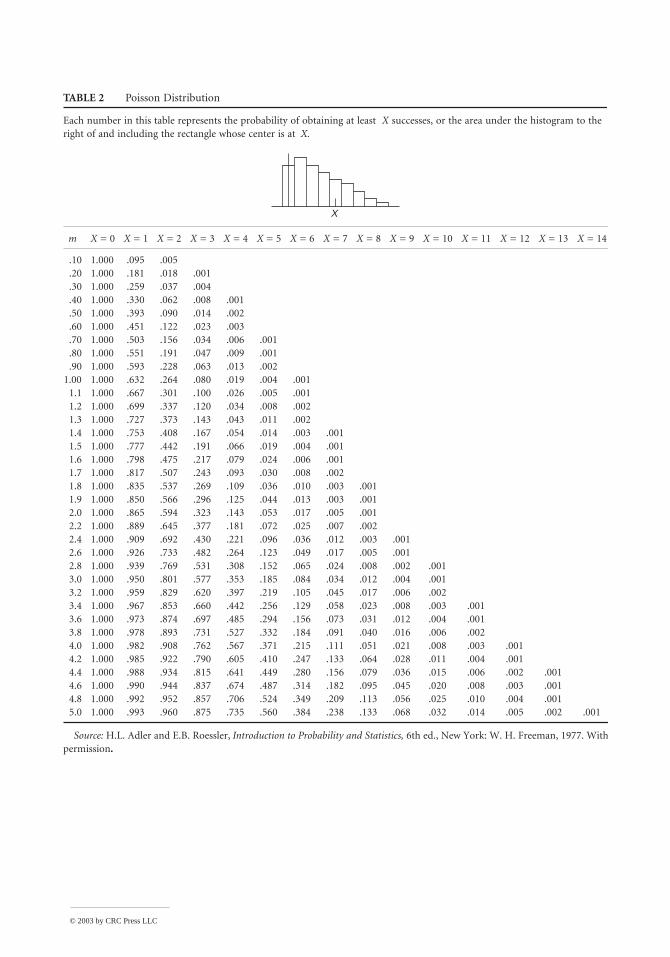
© 2003 by CRC Press LLC
TABLE 2 Poisson Distribution
Each number in this table represents the probability of obtaining at least X successes, or the area under the histogram to the right of and including the rectangle whose center is at X.
m X = 0 X = 1 X = 2 X = 3 X = 4 X = 5 X = 6 X = 7 X = 8 X = 9 X = 10 X = 11 X = 12 X = 13 X = 14
.10 1.000 .095 .005
.20 1.000 .181 .018 .001
.30 1.000 .259 .037 .004
.40 1.000 .330 .062 .008 .001
.50 1.000 .393 .090 .014 .002
.60 1.000 .451 .122 .023 .003
.70 1.000 .503 .156 .034 .006 .001
.80 1.000 .551 .191 .047 .009 .001
.90 1.000 .593 .228 .063 .013 .0021.00 1.000 .632 .264 .080 .019 .004 .001
1.1 1.000 .667 .301 .100 .026 .005 .0011.2 1.000 .699 .337 .120 .034 .008 .0021.3 1.000 .727 .373 .143 .043 .011 .0021.4 1.000 .753 .408 .167 .054 .014 .003 .0011.5 1.000 .777 .442 .191 .066 .019 .004 .0011.6 1.000 .798 .475 .217 .079 .024 .006 .0011.7 1.000 .817 .507 .243 .093 .030 .008 .0021.8 1.000 .835 .537 .269 .109 .036 .010 .003 .0011.9 1.000 .850 .566 .296 .125 .044 .013 .003 .0012.0 1.000 .865 .594 .323 .143 .053 .017 .005 .0012.2 1.000 .889 .645 .377 .181 .072 .025 .007 .0022.4 1.000 .909 .692 .430 .221 .096 .036 .012 .003 .0012.6 1.000 .926 .733 .482 .264 .123 .049 .017 .005 .0012.8 1.000 .939 .769 .531 .308 .152 .065 .024 .008 .002 .0013.0 1.000 .950 .801 .577 .353 .185 .084 .034 .012 .004 .0013.2 1.000 .959 .829 .620 .397 .219 .105 .045 .017 .006 .0023.4 1.000 .967 .853 .660 .442 .256 .129 .058 .023 .008 .003 .0013.6 1.000 .973 .874 .697 .485 .294 .156 .073 .031 .012 .004 .0013.8 1.000 .978 .893 .731 .527 .332 .184 .091 .040 .016 .006 .0024.0 1.000 .982 .908 .762 .567 .371 .215 .111 .051 .021 .008 .003 .0014.2 1.000 .985 .922 .790 .605 .410 .247 .133 .064 .028 .011 .004 .0014.4 1.000 .988 .934 .815 .641 .449 .280 .156 .079 .036 .015 .006 .002 .0014.6 1.000 .990 .944 .837 .674 .487 .314 .182 .095 .045 .020 .008 .003 .0014.8 1.000 .992 .952 .857 .706 .524 .349 .209 .113 .056 .025 .010 .004 .0015.0 1.000 .993 .960 .875 .735 .560 .384 .238 .133 .068 .032 .014 .005 .002 .001
Source: H.L. Adler and E.B. Roessler, Introduction to Probability and Statistics, 6th ed., New York: W. H. Freeman, 1977. With permission.
X
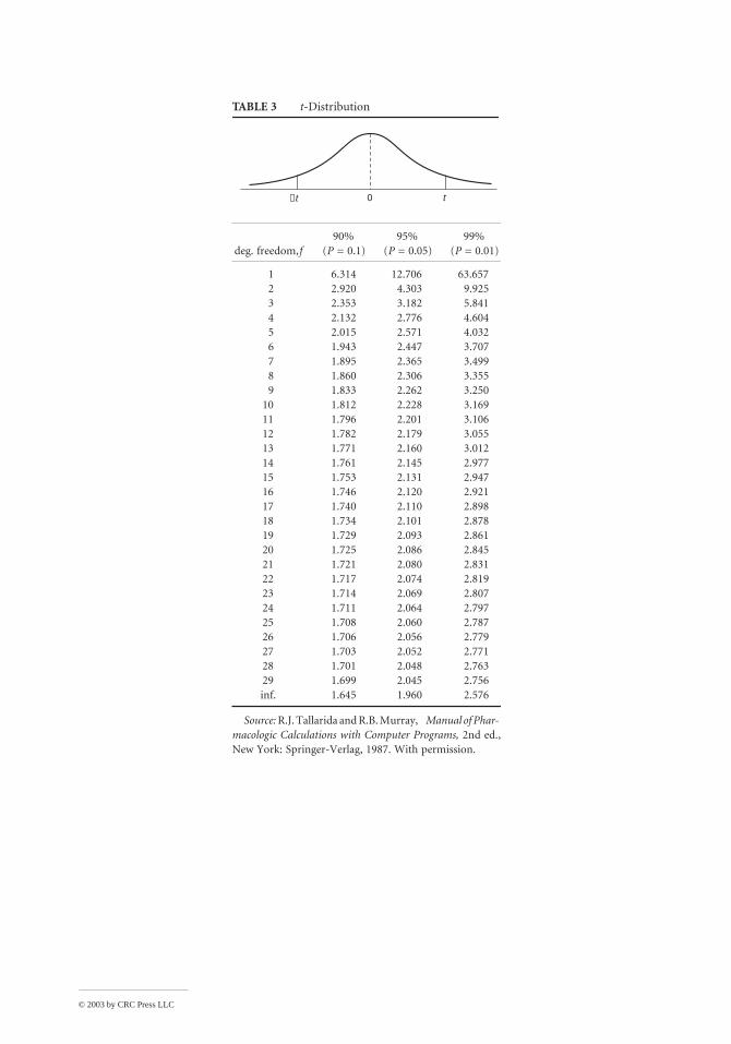
© 2003 by CRC Press LLC
TABLE 3 t-Distribution
deg. freedom, f90%
(P = 0.1)95%
(P = 0.05)99%
(P = 0.01)
1 6.314 12.706 63.6572 2.920 4.303 9.9253 2.353 3.182 5.8414 2.132 2.776 4.6045 2.015 2.571 4.0326 1.943 2.447 3.7077 1.895 2.365 3.4998 1.860 2.306 3.3559 1.833 2.262 3.250
10 1.812 2.228 3.16911 1.796 2.201 3.10612 1.782 2.179 3.05513 1.771 2.160 3.01214 1.761 2.145 2.97715 1.753 2.131 2.94716 1.746 2.120 2.92117 1.740 2.110 2.89818 1.734 2.101 2.87819 1.729 2.093 2.86120 1.725 2.086 2.84521 1.721 2.080 2.83122 1.717 2.074 2.81923 1.714 2.069 2.80724 1.711 2.064 2.79725 1.708 2.060 2.78726 1.706 2.056 2.77927 1.703 2.052 2.77128 1.701 2.048 2.76329 1.699 2.045 2.756inf. 1.645 1.960 2.576
Source: R.J. Tallarida and R.B. Murray, Manual of Phar-macologic Calculations with Computer Programs, 2nd ed., New York: Springer-Verlag, 1987. With permission.
−t t0
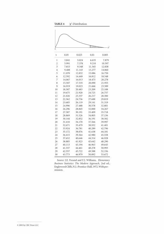
© 2003 by CRC Press LLC
TABLE 4 χ2-Distribution
v 0.05 0.025 0.01 0.005
1 3.841 5.024 6.635 7.879 2 5.991 7.378 9.210 10.597 3 7.815 9.348 11.345 12.838 4 9.488 11.143 13.277 14.860 5 11.070 12.832 15.086 16.750 6 12.592 14.449 16.812 18.548 7 14.067 16.013 18.475 20.278 8 15.507 17.535 20.090 21.955 9 16.919 19.023 21.666 23.589
10 18.307 20.483 23.209 25.18811 19.675 21.920 24.725 26.75712 21.026 23.337 26.217 28.30013 22.362 24.736 27.688 29.81914 23.685 26.119 29.141 31.31915 24.996 27.488 30.578 32.80116 26.296 28.845 32.000 34.26717 27.587 30.191 33.409 35.71818 28.869 31.526 34.805 37.15619 30.144 32.852 36.191 38.58220 31.410 34.170 37.566 39.99721 32.671 35.479 38.932 41.40122 33.924 36.781 40.289 42.79623 35.172 38.076 41.638 44.18124 36.415 39.364 42.980 45.55825 37.652 40.646 44.314 46.92826 38.885 41.923 45.642 48.29027 40.113 43.194 46.963 49.64528 41.337 44.461 48.278 50.99329 42.557 45.722 49.588 52.33630 43.773 46.979 50.892 53.672
Source: J.E. Freund and F.J. Williams, Elementary Business Statistics: The Modern Approach, 2nd ed., Englewood Cliffs, N.J.: Prentice-Hall, 1972. With per-mission.
X2
0
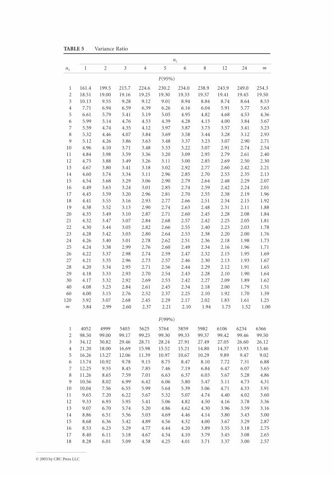
© 2003 by CRC Press LLC
TABLE 5 Variance Ratio
n1
n2 1 2 3 4 5 6 8 12 24 ∞
F(95%)
1 161.4 199.5 215.7 224.6 230.2 234.0 238.9 243.9 249.0 254.32 18.51 19.00 19.16 19.25 19.30 19.33 19.37 19.41 19.45 19.503 10.13 9.55 9.28 9.12 9.01 8.94 8.84 8.74 8.64 8.534 7.71 6.94 6.59 6.39 6.26 6.16 6.04 5.91 5.77 5.635 6.61 5.79 5.41 5.19 5.05 4.95 4.82 4.68 4.53 4.366 5.99 5.14 4.76 4.53 4.39 4.28 4.15 4.00 3.84 3.677 5.59 4.74 4.35 4.12 3.97 3.87 3.73 3.57 3.41 3.238 5.32 4.46 4.07 3.84 3.69 3.58 3.44 3.28 3.12 2.939 5.12 4.26 3.86 3.63 3.48 3.37 3.23 3.07 2.90 2.71
10 4.96 4.10 3.71 3.48 3.33 3.22 3.07 2.91 2.74 2.5411 4.84 3.98 3.59 3.36 3.20 3.09 2.95 2.79 2.61 2.4012 4.75 3.88 3.49 3.26 3.11 3.00 2.85 2.69 2.50 2.3013 4.67 3.80 3.41 3.18 3.02 2.92 2.77 2.60 2.42 2.2114 4.60 3.74 3.34 3.11 2.96 2.85 2.70 2.53 2.35 2.1315 4.54 3.68 3.29 3.06 2.90 2.79 2.64 2.48 2.29 2.0716 4.49 3.63 3.24 3.01 2.85 2.74 2.59 2.42 2.24 2.0117 4.45 3.59 3.20 2.96 2.81 2.70 2.55 2.38 2.19 1.9618 4.41 3.55 3.16 2.93 2.77 2.66 2.51 2.34 2.15 1.9219 4.38 3.52 3.13 2.90 2.74 2.63 2.48 2.31 2.11 1.8820 4.35 3.49 3.10 2.87 2.71 2.60 2.45 2.28 2.08 1.8421 4.32 3.47 3.07 2.84 2.68 2.57 2.42 2.25 2.05 1.8122 4.30 3.44 3.05 2.82 2.66 2.55 2.40 2.23 2.03 1.7823 4.28 3.42 3.03 2.80 2.64 2.53 2.38 2.20 2.00 1.7624 4.26 3.40 3.01 2.78 2.62 2.51 2.36 2.18 1.98 1.7325 4.24 3.38 2.99 2.76 2.60 2.49 2.34 2.16 1.96 1.7126 4.22 3.37 2.98 2.74 2.59 2.47 2.32 2.15 1.95 1.6927 4.21 3.35 2.96 2.73 2.57 2.46 2.30 2.13 1.93 1.6728 4.20 3.34 2.95 2.71 2.56 2.44 2.29 2.12 1.91 1.6529 4.18 3.33 2.93 2.70 2.54 2.43 2.28 2.10 1.90 1.6430 4.17 3.32 2.92 2.69 2.53 2.42 2.27 2.09 1.89 1.6240 4.08 3.23 2.84 2.61 2.45 2.34 2.18 2.00 1.79 1.5160 4.00 3.15 2.76 2.52 2.37 2.25 2.10 1.92 1.70 1.39
120 3.92 3.07 2.68 2.45 2.29 2.17 2.02 1.83 1.61 1.25∞ 3.84 2.99 2.60 2.37 2.21 2.10 1.94 1.75 1.52 1.00
F(99%)
1 4052 4999 5403 5625 5764 5859 5982 6106 6234 63662 98.50 99.00 99.17 99.25 99.30 99.33 99.37 99.42 99.46 99.503 34.12 30.82 29.46 28.71 28.24 27.91 27.49 27.05 26.60 26.124 21.20 18.00 16.69 15.98 15.52 15.21 14.80 14.37 13.93 13.465 16.26 13.27 12.06 11.39 10.97 10.67 10.29 9.89 9.47 9.026 13.74 10.92 9.78 9.15 8.75 8.47 8.10 7.72 7.31 6.887 12.25 9.55 8.45 7.85 7.46 7.19 6.84 6.47 6.07 5.658 11.26 8.65 7.59 7.01 6.63 6.37 6.03 5.67 5.28 4.869 10.56 8.02 6.99 6.42 6.06 5.80 5.47 5.11 4.73 4.31
10 10.04 7.56 6.55 5.99 5.64 5.39 5.06 4.71 4.33 3.9111 9.65 7.20 6.22 5.67 5.32 5.07 4.74 4.40 4.02 3.6012 9.33 6.93 5.95 5.41 5.06 4.82 4.50 4.16 3.78 3.3613 9.07 6.70 5.74 5.20 4.86 4.62 4.30 3.96 3.59 3.1614 8.86 6.51 5.56 5.03 4.69 4.46 4.14 3.80 3.43 3.0015 8.68 6.36 5.42 4.89 4.56 4.32 4.00 3.67 3.29 2.8716 8.53 6.23 5.29 4.77 4.44 4.20 3.89 3.55 3.18 2.7517 8.40 6.11 5.18 4.67 4.34 4.10 3.79 3.45 3.08 2.6518 8.28 6.01 5.09 4.58 4.25 4.01 3.71 3.37 3.00 2.57
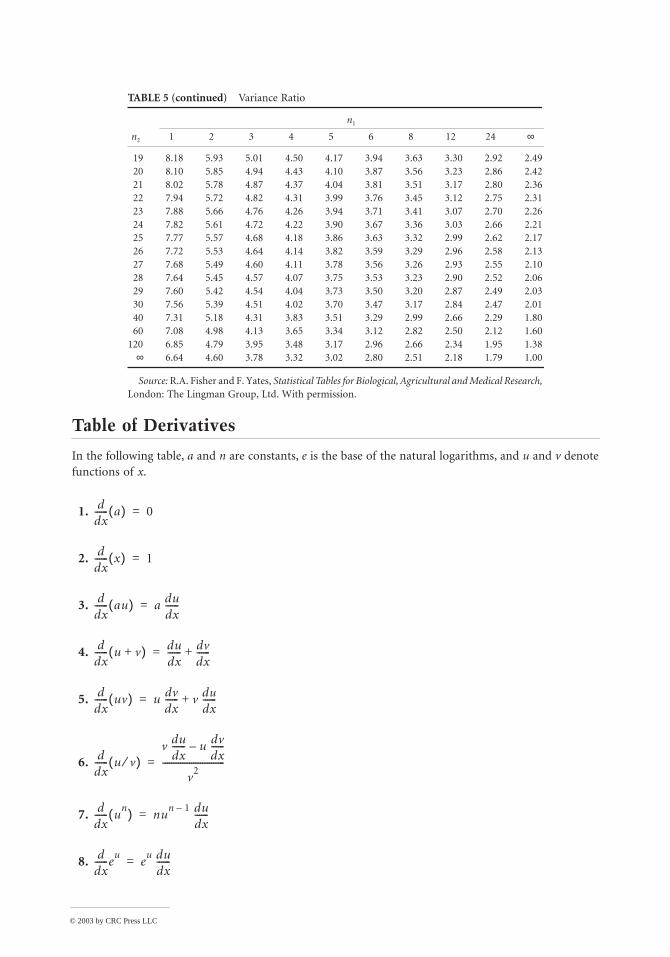
© 2003 by CRC Press LLC
Table of Derivatives
In the following table, a and n are constants, e is the base of the natural logarithms, and u and v denote functions of x.
1.
2.
3.
4.
5.
6.
7.
8.
TABLE 5 (continued) Variance Ratio
n1
n2 1 2 3 4 5 6 8 12 24 ∞
19 8.18 5.93 5.01 4.50 4.17 3.94 3.63 3.30 2.92 2.4920 8.10 5.85 4.94 4.43 4.10 3.87 3.56 3.23 2.86 2.4221 8.02 5.78 4.87 4.37 4.04 3.81 3.51 3.17 2.80 2.3622 7.94 5.72 4.82 4.31 3.99 3.76 3.45 3.12 2.75 2.3123 7.88 5.66 4.76 4.26 3.94 3.71 3.41 3.07 2.70 2.2624 7.82 5.61 4.72 4.22 3.90 3.67 3.36 3.03 2.66 2.2125 7.77 5.57 4.68 4.18 3.86 3.63 3.32 2.99 2.62 2.1726 7.72 5.53 4.64 4.14 3.82 3.59 3.29 2.96 2.58 2.1327 7.68 5.49 4.60 4.11 3.78 3.56 3.26 2.93 2.55 2.1028 7.64 5.45 4.57 4.07 3.75 3.53 3.23 2.90 2.52 2.0629 7.60 5.42 4.54 4.04 3.73 3.50 3.20 2.87 2.49 2.0330 7.56 5.39 4.51 4.02 3.70 3.47 3.17 2.84 2.47 2.0140 7.31 5.18 4.31 3.83 3.51 3.29 2.99 2.66 2.29 1.8060 7.08 4.98 4.13 3.65 3.34 3.12 2.82 2.50 2.12 1.60
120 6.85 4.79 3.95 3.48 3.17 2.96 2.66 2.34 1.95 1.38∞ 6.64 4.60 3.78 3.32 3.02 2.80 2.51 2.18 1.79 1.00
Source: R.A. Fisher and F. Yates, Statistical Tables for Biological, Agricultural and Medical Research,London: The Lingman Group, Ltd. With permission.
ddx------ a( ) 0=
ddx------ x( ) 1=
ddx------ au( ) a du
dx------=
ddx------ u v+( ) du
dx------ dv
dx------+=
ddx------ uv( ) u dv
dx------ v
dudx------+=
ddx------ u v⁄( )
vdudx------ u dv
dx------–
v2
----------------------------=
ddx------ u
n( ) nun 1– du
dx------=
ddx------e
ue
u dudx------=
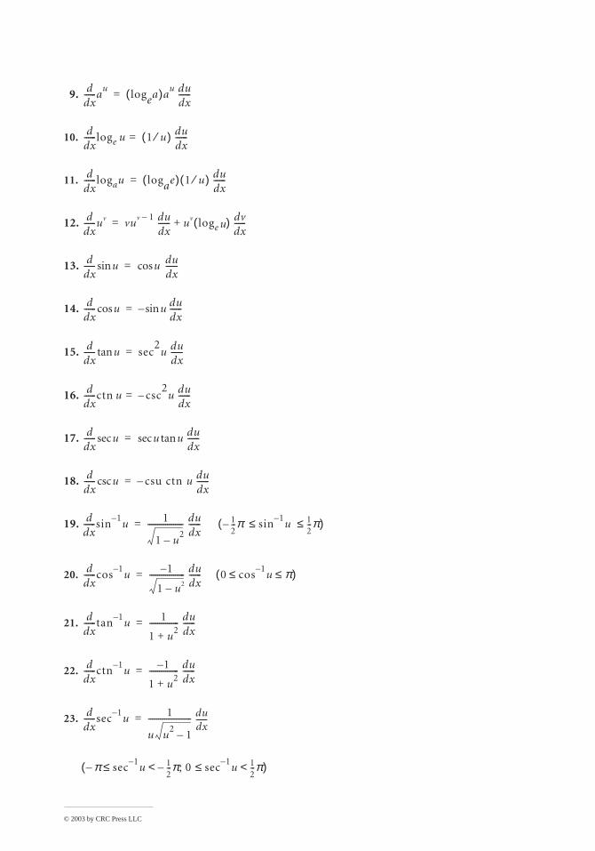
© 2003 by CRC Press LLC
9.
10.
11.
12.
13.
14.
15.
16.
17.
18.
19.
20.
21.
22.
23.
ddx------a
ulogea( )a
u dudx------=
ddx------ loge u 1 u⁄( ) du
dx------=
ddx------ logau logae( ) 1 u⁄( ) du
dx------=
ddx------uv
vuv 1– du
dx------ uv loge u( ) dv
dx------+=
ddx------ usin ucos du
dx------=
ddx------ ucos u du
dx------sin–=
ddx------ utan sec
2u du
dx------=
ddx------ctn u c– sc
2u du
dx------=
ddx------ usec u u du
dx------tansec=
ddx------ ucsc csu ctn u du
dx------–=
ddx------sin
1–u 1
1 u2
–------------------ du
dx------ 1
2 - - - π – sin
1
– u 1 2
- - - π ≤ ≤ ( ) =
ddx------cos
1–u 1–
1 u2–------------------ du
dx------ 0 cos
1
– u π ≤ ≤ ( ) =
ddx------tan
1–u 1
1 u2
+--------------- du
dx------=
ddx------ctn
1–u 1–
1 u2
+--------------- du
dx------=
ddx------sec
1–u 1
u u2
1–---------------------- du
dx------=
π– sec1–u≤ 1
2---π 0 ;–< sec
1–u≤ 1
2---π<( )
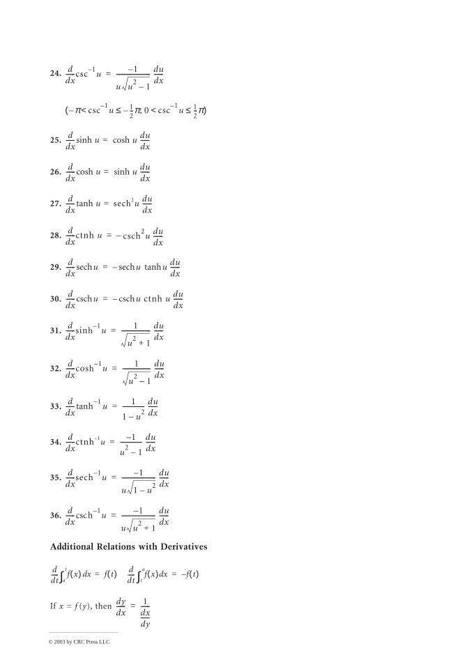
© 2003 by CRC Press LLC
24.
25.
26.
27.
28.
29.
30.
31.
32.
33.
34.
35.
36.
Additional Relations with Derivatives
If x = f (y), then
ddx------csc
1–u 1–
u u2
1–---------------------- du
dx------=
π– csc1–u< 1
2---π; 0– csc
1–u< 1
2---π≤ ≤( )
ddx------ usinh u du
dx------cosh=
ddx------ ucosh u du
dx------sinh=
ddx------ utanh sech2u du
dx------=
ddx------ctnh u csch
2u du
dx------–=
ddx------ usech u u du
dx------tanhsech–=
ddx------ ucsch u ctnh u du
dx------csch–=
ddx------sinh
1–u 1
u2
1+------------------- du
dx------=
ddx------cosh
1–u 1
u2
1–------------------ du
dx------=
ddx------ h
1–utan 1
1 u2
–-------------- du
dx------=
ddx------ctnh 1–
u1–
u2
1–-------------- du
dx------=
ddx------sech
1–u 1–
u 1 u2
–---------------------- du
dx------=
ddx------ h
1–ucsc 1–
u u2
1+
---------------------- dudx------=
ddt----- f x( ) xd
a
t
∫ f t( ) ddt----- f x( ) xd
t
a
∫ f t( )–= =
dydx------ 1
dxdy------------=
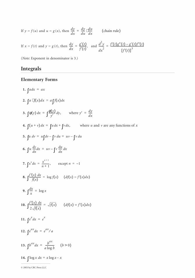
© 2003 by CRC Press LLC
If y = f (u) and u = g (x), then
If x = f (t) and y = g (t), then and
(Note: Exponent in denominator is 3.)
Integrals
Elementary Forms
1.
2.
3.
4.
5.
6.
7.
8.
9.
10.
11.
12.
13.
14.
dydx------ dy
du------ du
dx------ chain rule( )⋅=
dydx------ g ′ t( )
f ′ t( )-----------,= d
2y
dx2
-------- f ′ t( )g″ t( ) g ′ t( )f ″ t( )–
f ′ t( )[ ] 3----------------------------------------------------=
a xd∫ ax=
a∫ f x( )dx⋅ a f x( ) xd∫=
φ y( ) xd∫φ y( )
y ′---------- y, where y ′d∫
dydx------= =
u v+( ) xd∫ u xd∫ v x, where u and v are any functions of xd∫+=
u vd∫ u vd∫ v ud∫– uv v ud∫–= =
u vdxd
----- xd∫ uv vudxd
----- xd∫–=
xn xd∫ xn 1+
n 1+------------ , except n 1–= =
f ′ x( ) xdf x( )
-------------------∫ f x( ) df x( ) = f ′ x( )dx( )log=
xdx-----∫ xlog=
f ′ x( ) xd
2 f x( )-------------------∫ f x( ) df x( ) = f ′ x( )dx( )=
ex
xd∫ ex
=
eax
xd∫ eax
a⁄=
bax
xd∫b
ax
a blog-------------- b 0>( )=
xlog xd∫ x xlog x–=
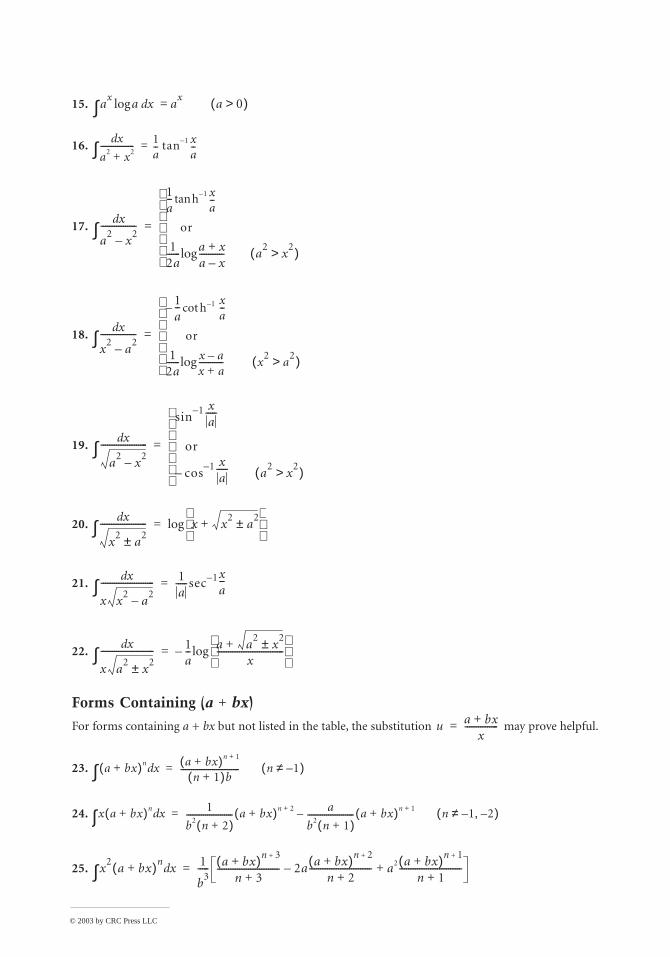
© 2003 by CRC Press LLC
15.
16.
17.
18.
19.
20.
21.
22.
Forms Containing (a + bx)
For forms containing a + bx but not listed in the table, the substitution may prove helpful.
23.
24.
25.
ax alog xd∫ a
xa 0>( )=
xd
a2 x2+----------------∫ 1
a-- tan 1– x
a--=
xd
a2
x2
–----------------∫
1a-- h 1– x
a--tan
or
12a------ a x+
a x–----------- a
2x
2>( )log
=
xd
x2
a2
–----------------∫
1a--– h 1–cot
xa--
or
12a------ x a–
x a+----------- x
2a
2>( )log
=
xd
a2
x2
–---------------------∫
sin1– x
a-----
or
cos1– x
a----- a
2x
2>( )–
=
xd
x2
a2±
---------------------∫ x x2
a2±+
log=
xd
x x2
a2
–------------------------∫
1a-----sec 1– x
a--=
xd
x a2
x2±
------------------------∫1a-- a a
2x
2±+x
------------------------------
log–=
u a bx+x
---------------=
a bx+( )n xd∫ a bx+( )n 1+
n 1+( )b---------------------------- n 1–≠( )=
x a bx+( )n xd∫ 1
b2 n 2+( )---------------------- a bx+( )n 2+ a
b2 n 1+( )---------------------- a bx+( )n 1+ n 1–≠ 2–,( )–=
x2
a bx+( )nxd∫
1
b3
----- a bx+( )n 3+
n 3+---------------------------- 2a a bx+( )n 2+
n 2+----------------------------– a2 a bx+( )n 1+
n 1+----------------------------+=
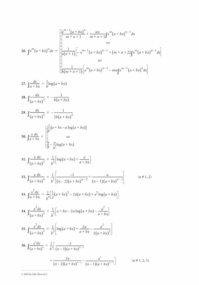
© 2003 by CRC Press LLC
26.
27.
28.
29.
30.
31.
32.
33.
34.
35.
36.
xm
a bx+( )nxd∫
xm 1+
a bx+( )n
m n 1+ +------------------------------------ an
m n 1+ +----------------------- x
ma bx+( )n 1–
xd∫+
or
1a n 1+( )-------------------- x
m 1+a bx+( )n 1+
– m n 2+ +( ) xm
a bx+( )n 1+xd∫+
or
1b m n 1+ +( )------------------------------- x
ma bx+( )n 1+
ma xm 1+
a bx+( )nxd∫–
=
xda bx+---------------∫
1b-- a bx+( )log=
xd
a bx+( )2----------------------∫
1b a bx+( )-----------------------–=
xd
a bx+( )3----------------------∫
1
2b a bx+( )2-----------------------------–=
x xda bx+---------------∫
1
b2---- a bx a a bx+( )log–+[ ]
or
xb-- a
b2---- a bx+( )log–
=
x xd
a bx+( )2----------------------∫
1
b2
----- a bx+( )log aa bx+---------------+=
x xd
a bx+( )n----------------------∫
1
b2
----- 1–
n 2–( ) a bx+( )n 2–----------------------------------------------- a
n 1–( ) a bx+( )n 1–-----------------------------------------------+ (n ≠ 1, 2)=
x2
xda bx+---------------∫
1
b3
----- 12-- a bx+( )2
2a a bx+( )– a2
a bx+( )log+=
x2
xd
a bx+( )2----------------------∫
1
b3
----- a bx 2a a bx+( )log– a2
a bx+---------------–+=
x2
xd
a bx+( )3----------------------∫
1
b3
----- a bx+( )log 2aa bx+--------------- a
2
2 a bx+( )2-------------------------–+=
x2 xd
a bx+( )n----------------------∫ 1
b3----
1–
n 3–( ) a bx+( )n 3–---------------------------------------------=
2a
n 2–( ) a bx+( )n 2–--------------------------------------------- a2
n 1–( ) a bx+( )n 1–--------------------------------------------- (n ≠ 1, 2, 3)–+
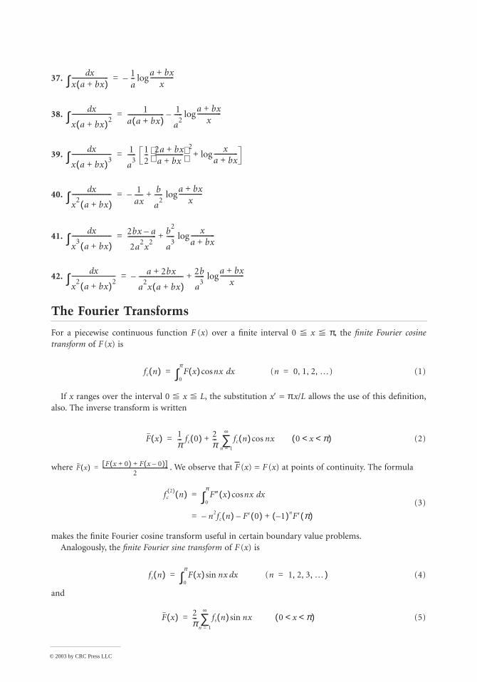
© 2003 by CRC Press LLC
37.
38.
39.
40.
41.
42.
The Fourier Transforms
For a piecewise continuous function F (x) over a finite interval 0 x π, the finite Fourier cosine transform of F (x) is
(1)
If x ranges over the interval 0 x L, the substitution x′ = π x/L allows the use of this definition, also. The inverse transform is written
(2)
where . We observe that F (x) = F (x) at points of continuity. The formula
(3)
makes the finite Fourier cosine transform useful in certain boundary value problems.Analogously, the finite Fourier sine transform of F (x) is
(4)
and
(5)
xdx a bx+( )-----------------------∫
1a--
a bx+x
---------------log–=
xd
x a bx+( )2-------------------------∫
1a a bx+( )----------------------- 1
a2
-----a bx+
x---------------log–=
xd
x a bx+( )3-------------------------∫
1
a3
----- 12-- 2a bx+
a bx+------------------
2 xa bx+---------------log+=
xd
x2
a bx+( )-------------------------∫
1ax-----– b
a2
-----a bx+
x---------------log+=
xd
x3
a bx+( )-------------------------∫
2bx a–
2a2x
2------------------ b
2
a3
-----x
a bx+---------------log+=
xd
x2
a bx+( )2----------------------------∫
a 2bx+
a2x a bx+( )
----------------------------– 2b
a3
------a bx+
x---------------log+=
fc n( ) F x( ) nxcos x (nd0
π
∫ 0 1 2 K), , ,= =
F x( ) 1π---
fc 0( ) 2π---
fc n( ) nx 0 x π< <( )cosn 1=
∞
∑+=
F x( ) F x 0+( ) F x 0–( )+[ ]2
----------------------------------------------------=
fc2( ) n( ) F″ x( ) nxcos xd
0
π
∫=
n2fc n( )– F ′ 0( )– 1–( )nF ′ π( )+=
fs n( ) F x( ) nxsin x (nd0
π
∫ 1 2 3 K ), , ,= =
F x( ) 2π---
fs n( ) nx 0 x π< <( )sinn 1=
∞
∑=
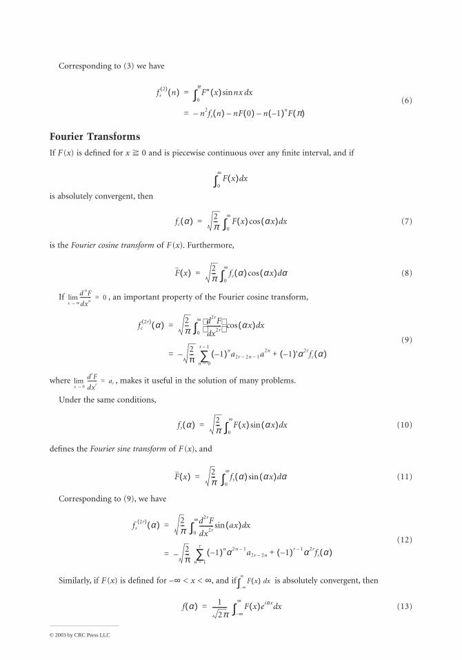
© 2003 by CRC Press LLC
Corresponding to (3) we have
(6)
Fourier Transforms
If F (x) is defined for x 0 and is piecewise continuous over any finite interval, and if
is absolutely convergent, then
(7)
is the Fourier cosine transform of F (x). Furthermore,
(8)
If , an important property of the Fourier cosine transform,
(9)
where , makes it useful in the solution of many problems.
Under the same conditions,
(10)
defines the Fourier sine transform of F (x), and
(11)
Corresponding to (9), we have
(12)
Similarly, if F (x) is defined for – ∞ < x < ∞, and if is absolutely convergent, then
(13)
fs2( ) n( ) F″ x( ) nxsin xd
0
π
∫=
n2fs n( )– nF 0( )– n 1–( )nF π( )–=
F x( ) xd0
∞
∫
fc α( ) 2π--- F x( ) αx( )cos xd
0
∞
∫=
F x( ) 2π--- fc α( ) αx( )cos αd
0
∞
∫=
d nF
dxn---------
x ∞→lim 0=
fc2r( ) α( ) 2
π---d2rF
x2rd----------
αx( )cos xd0
∞
∫=
2π--- 1–( )na2r 2n– 1– a2n 1–( )'α 2rfc α( )+
n 0=
r 1–
∑–=
drF
dxr--------
x 0→lim ar=
fs α( ) 2π--- F x( ) αx( )sin xd
0
∞
∫=
F x( ) 2π--- fs α( ) αx( )sin αd
0
∞
∫=
fs2r( ) α( ) 2
π--- d2rF
dx2r---------- ax( )sin xd
0
∞
∫=
2π---– 1–( )nα 2n 1– a2r 2n– 1–( )r 1– α 2rfs α( )+
n 1=
r
∑=
F x( ) xd∞–
∞
∫
f α( ) 1
2π---------- F x( )eiα x xd
∞–
∞
∫=
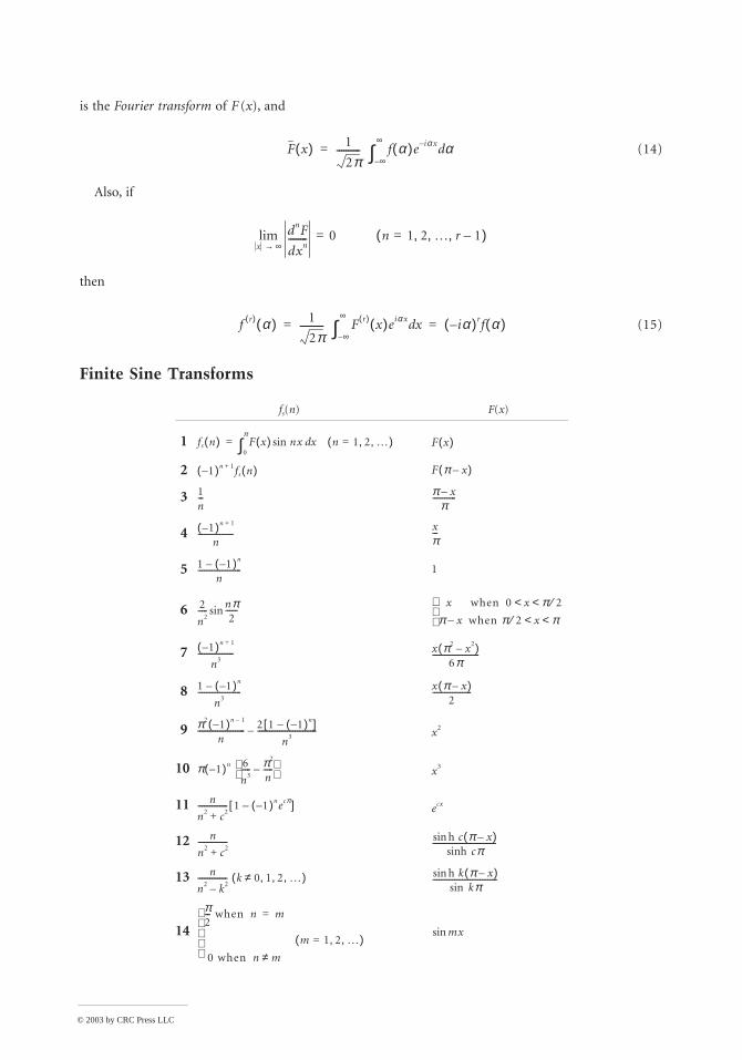
© 2003 by CRC Press LLC
is the Fourier transform of F (x), and
(14)
Also, if
then
(15)
Finite Sine Transforms
fs(n) F(x)
1
2
3
4
5
6
7
8
9
10
11
12
13
14
F x( ) 1
2π---------- f α( )e i– α x αd
∞–
∞
∫=
dnF
dxn--------
x ∞→lim 0= n 1 2 K r 1–, , ,=( )
f r( ) α( ) 1
2π---------- F r( ) x( )eiα x xd
∞–
∞
∫ iα–( )rf α( )= =
fs n( ) F x( ) nxsin x n 1 2 K, ,=( )d0
π
∫= F x( )
1–( )n 1+ fs n( ) F π x–( )
1n--- π x–
π------------
1–( )n 1+
n------------------
xπ---
1 1–( )n–n
---------------------- 1
2
n2----- nπ
2------sin
x when 0 x π 2⁄< <π x when π 2⁄ x π< <–
1–( )n 1+
n3------------------ x π2 x2–( )
6π------------------------
1 1–( )– n
n3---------------------- x π x–( )
2--------------------
π2 1–( )n 1–
n------------------------ 2 1 1–( )n–[ ]
n3------------------------------– x2
π 1–( )n 6
n3----- π2
n-----–
x3
n
n2 c2+--------------- 1 1–( )necπ–[ ] ecx
n
n2 c2+--------------- h c π x–( )sin
cπsinh--------------------------------
n
n2 k2–--------------- k 0 1 2 K, , ,≠( ) h k π x–( )sin
sin kπ---------------------------------
π2--- when n m=
m 1 2 K, ,=( )0 when n m≠
mxsin
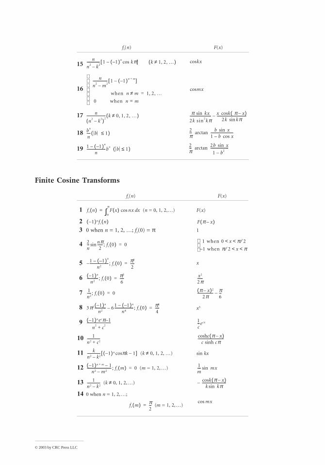
© 2003 by CRC Press LLC
Finite Cosine Transforms
15
16
17
18
19
fc(n) F(x)
1 (n = 0, 1, 2, K) F(x)
23 0 when n = 1, 2, K; fc(0) = π 1
4
5 x
6
7
8 x3
9
10
11 (k ≠ 0, 1, 2, K) sin kx
12 (m = 1, 2, K)
13 (k ≠ 0, 1, 2, K)
14 0 when n = 1, 2, K;
(m = 1, 2, K)
fs(n) F(x)
n
n2 k2–--------------- 1 1–( )n kπcos–[ ] k 1 2 K, ,≠( ) kxcos
n
n2 m2–----------------- 1 1–( )n m+–[ ]
when n m≠ 1 2 K, ,=
0 when n m=
mxcos
n
n2 k2–( )2---------------------- k 0 1 2 K, , ,≠( ) π kxsin
2k sin2kπ------------------------- x kcos π x–( )
2k kπsin----------------------------------–
bn
n---- b 1≤( ) 2
π--- arctan b xsin
1 b xcos–--------------------------
1 1–( )n–n
----------------------bn b 1≤( )2π--- arctan 2b xsin
1 b2 –---------------------
fc n( ) F x( ) nxcos xd0
π
∫=
1–( )nfc n( ) F π x–( )
2n--- nπ
2------ fc 0( );sin 0=
1 when 0 x π 2⁄< <1 when π 2⁄ x π< <–
1 1–( )n–n2
---------------------- fc 0( );– π2
2-----=
1–( )n
n2------------- fc 0( ); π2
6-----= x2
2π------
1n2----- fc 0( ); 0= π x–( )2
2π------------------ π
6---–
3π2 1–( )n
n2------------- 6 1 1–( )n–
n4---------------------- fc 0( );– π4
4-----=
1–( )necπ 1–
n2 c2+---------------------------- 1
c---ecx
1n2 c2+--------------- c π x–( )cosh
c cπsinh------------------------------
kn2 k2–--------------- 1–( )n πk 1–cos[ ]
1–( )n m+ 1–n2 m2–
---------------------------- fc m( ); 0= 1m---- mxsin
1n2 k2–--------------- k π x–( )cos
k kπsin----------------------------–
fc m( ) π2---=
mxcos
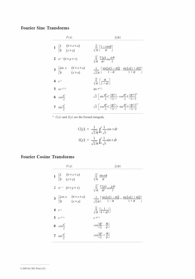
© 2003 by CRC Press LLC
Fourier Sine Transforms
Fourier Cosine Transforms
F (x) fs(α)
1
2
3
4
5
6
7
* C(y) and S(y) are the Fresnel integrals.
F (x) fc(α)
1
2
3
4
5
6
7
1 0 x a< <( )0 x a>( )
2
π--- 1 αcos–
α---------------------
xp 1– 0 p 1< <( ) 2π--- Γ p( )
α p----------- pπ
2------sin
x 0 x a< <( )sin
0 x a>( ) 1
2π---------- a 1 α–( )[ ]sin
1 α–---------------------------------- a 1 α+( )[ ]sin
1 α+----------------------------------–
e x– 2π--- α
1 α 2+---------------
xe x2 2⁄– α e α2 2⁄–
x2
2----cos 2 α 2
2-----C α 2
2-----
α 2
2-----S α 2
2-----
cos–sin*
x2
2----sin 2
α 2
2-----cos C α 2
2-----
α 2
2-----sin S α 2
2-----
+*
C y( ) 1
2π----------
1
t----- tcos td
0
y
∫=
S y( ) 1
2π----------
1
t----- t tdsin
0
y
∫=
1 0 x a< <( )0 x a>( )
2
π--- aαsin
α---------------
xp 1– 0 p 1< <( ) 2π--- Γ p( )
α p----------- pπ
2------cos
x 0 x a< <( )cos
0 x a>( ) 1
2π---------- a 1 α–( )[ ]sin
1 α–---------------------------------- a 1 α+( )[ ]sin
1 α+----------------------------------+
e x– 2π--- 1
1 α 2+---------------
e x2 2⁄– e α2 2⁄–
x2
2----cos
α 2
2----- π
4---–
cos
x2
2----sin
α 2
2----- π
4---+
cos
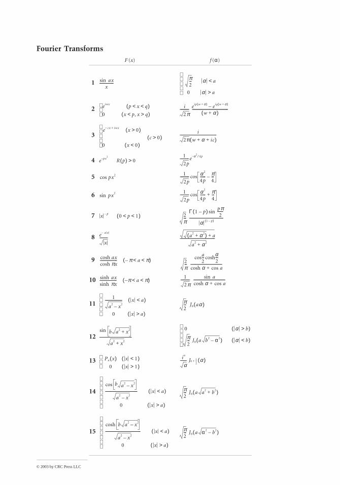
© 2003 by CRC Press LLC
Fourier TransformsF (x) f (α)
1
2
3
4
5
6
7
8
9
10
11
12
13
14
15
axsinx
----------------π2--- α a<
0 α a>
eiwx p x q< <( )0 x p x q>,<( )
i
2π---------- eip w α+( ) eiq w α+( )–
w α+( )----------------------------------------
e cx– iwx+ x 0>( )c 0>( )
0 x 0<( )
i
2π w α ic+ +( )-----------------------------------------
e px2
– R p( ) 0>1
2p----------e α2
4p⁄–
px2cos1
2p---------- α 2
4p------ π
4---–cos
px2sin1
2p---------- α 2
4p------ π
4---+cos
x p– 0 p 1< <( ) 2π---
Γ 1 p–( ) pπ2
------sin
α 1 p–( )--------------------------------------
e a x–
x--------- a2 α 2+( ) a+
a2 α 2+---------------------------------------
axcosh πxcosh
------------------- π a π< <–( ) 2π---
a2--- α
2---coshcos
α acos+cosh-----------------------------------
axsinh πxsinh
------------------- π a π< <–( ) 1
2π---------- asin
α acos+cosh-----------------------------------
1
a2 x2–------------------- x a<( )
0 x a>( )
π2--- J0 aα( )
b a2 x2+sin
a2 x2+------------------------------------
0 α b>( )
π2--- J0 a b2 α 2–( ) α b<( )
Pn x( ) x 1<( )0 x 1>( )
in
α------- Jn 1
2--+ α( )
b a2 x2–cos
a2 x2–------------------------------------ x a<( )
0 x a>( )
π2--- J0 a a2 b2+( )
h b a2 x2–cos
a2 x2–--------------------------------------- x a<( )
0 x a>( )
π2--- J0 a α 2 b2–( )
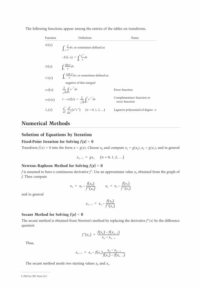
© 2003 by CRC Press LLC
The following functions appear among the entries of the tables on transforms.
Numerical Methods
Solution of Equations by Iteration
Fixed-Point Iteration for Solving f (x) = 0
Transform f (x) = 0 into the form x = g(x). Choose x0 and compute x1 = g(x0), x2 = g(x1), and in general
Newton–Raphson Method for Solving f (x) = 0
f is assumed to have a continuous derivative f ′. Use an approximate value x0 obtained from the graph of f. Then compute
and in general
Secant Method for Solving f (x) = 0
The secant method is obtained from Newton’s method by replacing the derivative f ′(x) by the difference quotient
Thus,
The secant method needs two starting values x0 and x1.
Function Definition Name
Error function
Complementary function to error function
Laguerre polynomial of degree n
Ei x( ) ev
v---- v ; or sometimes defined asd
∞–
x
∫
Ei x–( )– e v–
v------ vd
x
∞
∫=
Si x( ) vsinv
---------- vd0
x
∫
Ci x( ) vcos
v------------ v ; or sometimes defined asd
∞
x
∫negative of this integral
erf x( )2
π------- e v–
2
vd0
x
∫
erfc x( ) 1 erf x( )– 2
π------- e v
2– vd
x
∞
∫=
Ln x( ) ex
n!----- dn
dxn-------- xne x–( ) n = 0, 1, 2, …( )
xn 1+ gxn n = 0, 1, 2, …( )=
x1 x0f x0( )
f ′ x0( )-------------- x2,– x1
f x1( )f ′ x1( )--------------–= =
xn 1+ xn
f x0( )f ′ xn( )--------------–=
f ′ xn( )f xn( ) f xn 1–( )–
xn xn 1––----------------------------------=
xn 1+ xn f xn( ) xn xn 1––f xn( ) f xn 1–( )–----------------------------------–=
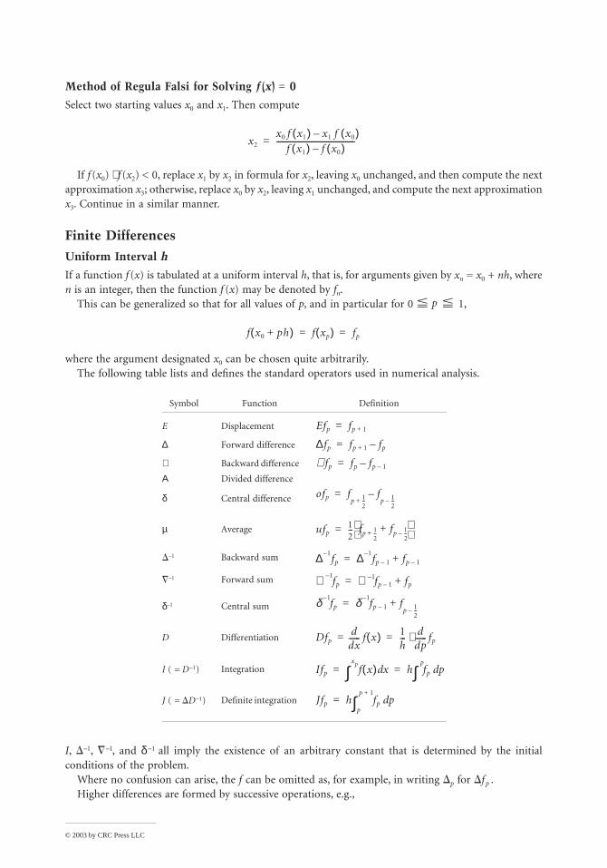
© 2003 by CRC Press LLC
Method of Regula Falsi for Solving f (x) = 0
Select two starting values x0 and x1. Then compute
If f (x0) ⋅ f (x2) < 0, replace x1 by x2 in formula for x2, leaving x0 unchanged, and then compute the next approximation x3; otherwise, replace x0 by x2, leaving x1 unchanged, and compute the next approximation x3. Continue in a similar manner.
Finite Differences
Uniform Interval h
If a function f (x) is tabulated at a uniform interval h, that is, for arguments given by xn = x0 + nh, where n is an integer, then the function f (x) may be denoted by fn.
This can be generalized so that for all values of p, and in particular for 0 p 1,
where the argument designated x0 can be chosen quite arbitrarily.The following table lists and defines the standard operators used in numerical analysis.
I, –1, –1, and δ–1 all imply the existence of an arbitrary constant that is determined by the initial conditions of the problem.
Where no confusion can arise, the f can be omitted as, for example, in writing p for f p .Higher differences are formed by successive operations, e.g.,
Symbol Function Definition
E Displacement
∆ Forward difference
∇ Backward difference
Α Divided difference
δ Central difference
µ Average
–1 Backward sum
–1 Forward sum
δ–1 Central sum
D Differentiation
I ( = D–1) Integration
J ( = D–1) Definite integration
x2
x0 f x1( ) x1 f x0( )–f x1( ) f x0( )–
-----------------------------------------=
f x0 ph+( ) f xp( ) fp= =
Efp fp 1+=
∆fp fp 1+ fp–=
∇ fp fp fp 1––=
ofp fp 1
2--+
fp 1
2--–
–=
ufp12--- fp 1
2--+ fp 1
2--–+
=
∆ 1–fp ∆ 1–
fp 1– fp 1–+=
∇ 1–fp ∇ 1– fp 1– fp+=
δ 1–fp δ 1–
fp 1– fp 1
2--–
+=
Dfpd
dx------ f x( ) 1
h---
ddp------ fp⋅= =
Ifp f x( ) xdxp
∫ h fp pdp
∫= =
Jfp h fp pdp
p 1+
∫=
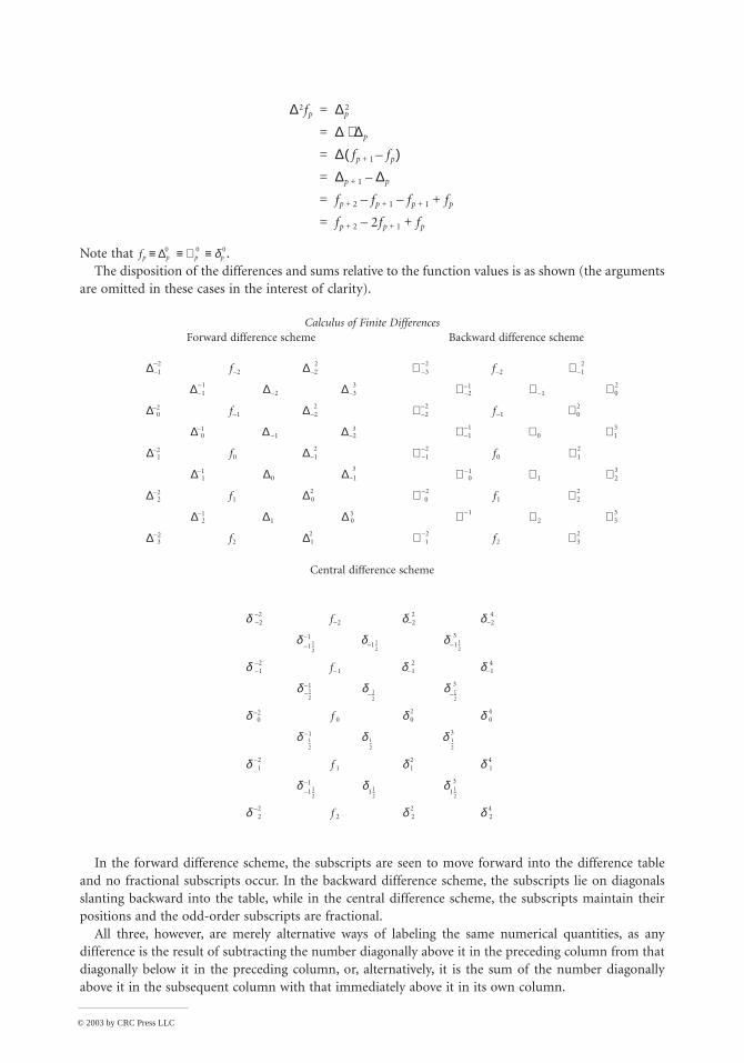
© 2003 by CRC Press LLC
Note that .The disposition of the differences and sums relative to the function values is as shown (the arguments
are omitted in these cases in the interest of clarity).
In the forward difference scheme, the subscripts are seen to move forward into the difference table and no fractional subscripts occur. In the backward difference scheme, the subscripts lie on diagonals slanting backward into the table, while in the central difference scheme, the subscripts maintain their positions and the odd-order subscripts are fractional.
All three, however, are merely alternative ways of labeling the same numerical quantities, as any difference is the result of subtracting the number diagonally above it in the preceding column from that diagonally below it in the preceding column, or, alternatively, it is the sum of the number diagonally above it in the subsequent column with that immediately above it in its own column.
Calculus of Finite DifferencesForward difference scheme Backward difference scheme
Central difference scheme
∆2fp ∆p2=
∆ ∆p⋅=
∆ fp 1+ fp–( )=
∆= p 1+ ∆p–
f= p 2+ fp 1+– fp 1+– fp+
f= p 2+ 2fp 1+– fp+
fp ∆p0 ∇ p
0 δp0≡ ≡ ≡
∆ 1–2– f 2– ∆ 2–
2
∆ 1–1– ∆ 2– ∆ 3–
3
∆ 02– f 1– ∆ 2–
2
∆ 01– ∆ 1– ∆ 2–
3
∆ 12– f0 ∆ 1–
2
∆ 11– ∆0 ∆ 1–
3
∆ 22– f1 ∆ 0
2
∆ 21– ∆1 ∆ 0
3
∆ 32– f2 ∆1
2
∇ 3–2– f 2– ∇ 1–
2
∇ 2–1– ∇ 1– ∇ 0
2
∇ 2–2– f 1– ∇ 0
2
∇ 1–1– ∇ 0 ∇ 1
3
∇ 1–2– f0 ∇ 1
2
∇ 01– ∇ 1 ∇ 2
3
∇ 02– f1 ∇ 2
2
∇ 1– ∇ 2 ∇ 33
∇ 12– f2 ∇ 3
2
δ 2–2– f 2– δ 2–
2 δ 2–4
δ11
2--–
1– δ 112--– δ 11
2--–
3
δ 1–2– f 1– δ 1–
2 δ 1–4
δ 12--–1– δ 1
2--–
δ 12--–
3
δ 02– f 0 δ 0
2 δ 04
δ 12--
1– δ 12--
δ 12--
3
δ 12– f 1 δ 1
2 δ 14
δ11
2--–
1– δ11
2--
δ11
2--
3
δ 22– f 2 δ 2
2 δ 24
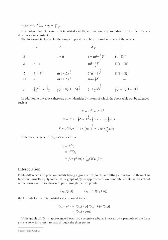
© 2003 by CRC Press LLC
In general,
If a polynomial of degree r is tabulated exactly, i.e., without any round-off errors, then the r th differences are constant.
The following table enables the simpler operators to be expressed in terms of the others:
In addition to the above, there are other identities by means of which the above table can be extended, such as
Note the emergence of Taylor’s series from
Interpolation
Finite difference interpolation entails taking a given set of points and fitting a function to them. This function is usually a polynomial. If the graph of f (x) is approximated over one tabular interval by a chord of the form y = a + bx chosen to pass through the two points
the formula for the interpolated value is found to be
If the graph of f (x) is approximated over two successive tabular intervals by a parabola of the form y = a + bx + cx2 chosen to pass through the three points
∆np 1
2--n– δp
n ∇ p 12--n+
.n≡ ≡
E ∆ δ µ, ∇
E –– 1 ∆+ 1 µδ 12---δ2
+ + 1 ∇–( ) 1–
∆ E 1– –– µδ 12---δ 2
+ ∇ 1 ∇–( ) 1–
δ E12--
E12--–
– ∆ 1 ∆+( )12--–
2 µ2 1–( )12--
∇ 1 ∇–( )12--–
∇ E 1–– ∆ 1 ∆+( ) 1– µδ 12---δ
2– ––
µ 12--- E
12--
E12--–+
12--- 2 ∆+( ) 1 ∆+( )
12--–
1 14---δ 2+( )
12--
12--- 2 ∇–( ) 1 ∇–( )
12--–
E ehD ∆∇ 1–= =
µ E12 ----– 1
2---δ+ E
12--
12---δ– 1
2---hD( )cosh= = =
δ E12--– ∆ E
12--
∇ ∆ ∇( )12--
= = 2 12---hD( )sinh= =
fp Epf0=
ephDf0=
f0 phDf012!----p2h2D2f0 L+ + +=
x0 f x0( ),( ) x0 h f x0 h+( ),+( ),
f x0 ph+( ) f x0( ) p f x0 h+( ) f x0( )–[ ]+=
f x0( ) p∆f0+=
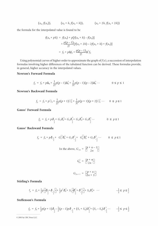
© 2003 by CRC Press LLC
the formula for the interpolated value is found to be
Using polynomial curves of higher order to approximate the graph of f (x), a succession of interpolation formulas involving higher differences of the tabulated function can be derived. These formulas provide, in general, higher accuracy in the interpolated values.
Newton’s Forward Formula
Newton’s Backward Formula
Gauss’ Forward Formula
Gauss’ Backward Formula
Stirling’s Formula
Steffenson’s Formula
x0 f x0( ),( ) x0 h f x0 h+( ),+( ), x0 2h f x0 2h+( ),+( ),
f x0 ph+( ) f x0( ) p f x0 h+( ) f x0( )–[ ]+=
p p 1–( )2!
------------------- f x0 2h+( ) 2f x0 h+( )– f x0( )+[ ]+
f0 p f0p p 1–( )
2!-------------------∆2f0+∆+=
fp f0 p∆012!----p p 1–( )∆0
2 13!----p p 1–( ) p 2–( )∆0
3 L 0 p 1≤ ≤+ + +=
fp f0 p∇ 012!----p p 1+( )∇ 0
2 13!----p p 1+( ) p 2+( )∇ 0
3 L 0 p 1≤≤+ + +=
fp f0 pδ 12--
G2δ02
G3δ 12--
3G4δ 0
4G5δ 1
2--
5 L 0 p 1≤≤+ + + + +=
fp f0 pδ 12--– G∗
2 δ02 G3δ 1
2--–
3 G∗4 δ0
4 G5δ 12--–
5 L 0 p 1≤≤+ + + + +=
In the above, G 2np n 1–+
2n =
G∗2n
p n+2n
=
G2n 1+p n+
2n 1+ =
fp f012---p δ1
2--
δ 12--–
+ 1
2---p2δ0
2S3 δ1
2--
3 δ 12--–
3+ S4δ 0
4 L 12--- p 1
2---≤ ≤–+ + + + +=
fp f012---p p 1+( )δ1
2--
12--- p 1–( )pδ 1
2--–
– S3 S4+( )δ12--
3 S3 S4–( )δ 12--–
3L 1
2--- p 1
2---≤ ≤–+ + +=

© 2003 by CRC Press LLC
Bessel’s Formula
Everett’s Formula
The coefficients in the above two formulae are related to each other and to the coefficients in the Gaussian formulae by the identities
Also, for q 1 – p the following symmetrical relationships hold:
as can be seen from the tables of these coefficients.
Bessel’s Formula (Unmodified)
In the above, S2n 1+12-- p n+
2n 1+ =
S2n 2+p
2n 2+--------------- p n+
2n 1+ =
S2n 1+ S2n 2++ p n 1+ +2n 2+
=
S2n 1+ S2n 2+– p n+2n 2+
–=
fp f0 pδ12--
B2 δ0
2δ1
2+
B3δ12--
3B4 δ 0
4 δ14
+( ) B5δ12--
5L 0 p 1≤≤+ + + + + +=
fp 1 p–( )f0 pf1 E2δ0
2F2δ1
2E4δ0
4F4δ1
4E6δ0
6F6δ1
6L 0 p 1≤≤+ + + + + + + +=
B2n 12---G2n
12--- E2n F2n+( )≡≡
B2n 1+ G2n 1+12---G2n
12--- F2n E2n–( )≡–≡
E2n G2n G2n 1+ B2n B2n 1+–≡–≡F2n G2n 1+ B2n B2n 1++≡ ≡
B2n p( ) B2n q( )≡B2n 1+ p( ) B– 2n 1+ q( )≡
E2n p( ) F2n q( )≡F2n p( ) E2n q( )≡
fp f0 pδ12--
B2 δ0
2δ1
2+
B3δ12--
3B4 δ0
4δ1
4+( ) B5δ1
2--
5B6 δ0
6δ1
6+
B7δ12--
7L+ + + + + + + +=
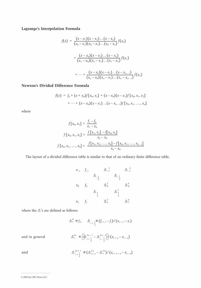
© 2003 by CRC Press LLC
Lagrange’s Interpolation Formula
Newton’s Divided Difference Formula
where
The layout of a divided difference table is similar to that of an ordinary finite difference table.
where the ’s are defined as follows:
and in general
and
f x( ) x x1–( ) x x2–( )… x xn–( )x0 x1–( ) x0 x2–( )… x0 xn–( )
-------------------------------------------------------------------- f x0( )=
x x0–( ) x x2–( )… x xn–( )x1 x0–( ) x1 x2–( )… x1 xn–( )
--------------------------------------------------------------------+ f x1( )
Lx x0–( ) x x1–( )… x xn 1––( )
xn x0–( ) xn x1–( )… xn xn 1––( )-------------------------------------------------------------------------- f xn( )+ +
f x( ) f0 x x0+( )f x0 x1,[ ] x x0–( ) x x1–( )f x0 x1 x2, ,[ ]+ +=
L x x0–( ) x x1–( )… x xn 1––( )f x0 x1, …, xn,[ ]+ +
f x0 x1,[ ]f1 f0–x1 x0–---------------=
f x0 x1 x2, ,[ ]f x1 x2,[ ] f x0 x1,[ ]–
x2 x0–------------------------------------------------=
f x0 x1, …, xk,[ ] f x1 x2, …, xk,[ ] f x0 x1, …, xk 1–,[ ]–
xk x0–------------------------------------------------------------------------------------------=
x 1– f 1– 1–2
1–4
12--–
12--–
x0 f0 02
04
12--
12--
3
x1 f1 12
14
0r fr
r 12--+
fr 1+ fr–( ) xr 1+ xr–( )⁄≡,≡
r2n
r 1
2--+
2n 1–
r 12--–
2n 1–– xr n+ xr n––( )⁄≡
2n 1+
r 12--+
r 1+2n
r2n–( ) xr 1 n+ + xr n––( )⁄≡
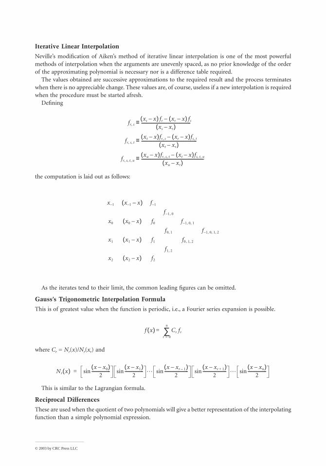
© 2003 by CRC Press LLC
Iterative Linear Interpolation
Neville’s modification of Aiken’s method of iterative linear interpolation is one of the most powerful methods of interpolation when the arguments are unevenly spaced, as no prior knowledge of the order of the approximating polynomial is necessary nor is a difference table required.
The values obtained are successive approximations to the required result and the process terminates when there is no appreciable change. These values are, of course, useless if a new interpolation is required when the procedure must be started afresh.
Defining
the computation is laid out as follows:
As the iterates tend to their limit, the common leading figures can be omitted.
Gauss’s Trigonometric Interpolation Formula
This is of greatest value when the function is periodic, i.e., a Fourier series expansion is possible.
where Cr = Nr(x)/Nr(xr) and
This is similar to the Lagrangian formula.
Reciprocal Differences
These are used when the quotient of two polynomials will give a better representation of the interpolating function than a simple polynomial expression.
fr s,xs x–( ) fr xr x–( ) fs–
xs xr–( )------------------------------------------------≡
fr s t, ,xt x–( )fr s, xr x–( )fs t,–
xt xr–( )------------------------------------------------------≡
fr s t u, , ,xu x–( )fr s t, , xt x–( )fs t u, ,–
xu xr–( )-------------------------------------------------------------≡
x 1– x 1– x–( ) f 1–
f 1, 0–
x0 x0 x–( ) f0 f 1 0 1, ,–
f0 1, f 1 0 1 2, , ,–
x1 x1 x–( ) f1 f0, 1, 2
f1 2,
x2 x2 x–( ) f2
f x( ) Cr frr 0=
n
∑=
Nr x( )x x0–( )
2------------------sin
x x1–( )2
------------------sin Lx xr 1––( )
2-----------------------sin
x xr 1+–( )2
-----------------------sin Lx xn–( )
2------------------sin=
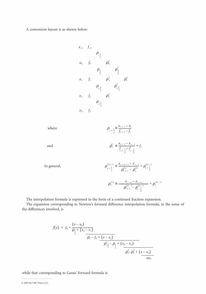
© 2003 by CRC Press LLC
A convenient layout is as shown below:
The interpolation formula is expressed in the form of a continued fraction expansion.The expansion corresponding to Newton’s forward difference interpolation formula, in the sense of
the differences involved, is
while that corresponding to Gauss’ forward formula is
x 1– f 1–
ρ 12--–
x0 f0 ρ02
ρ 12--
ρ 12--
3
x1 f1 ρ 12 ρ1
4
ρ1 1
2--
ρ1 1
2--
3
x2 f2 ρ22
ρ2 1
2--
x3 f3
where ρr 1
2--+
xr 1+ xr–fr 1+ fr–--------------------≡
and ρr2 xr 1+ xr 1––
fr 1
2--+
fr 1
2--–
–------------------------- fr+≡
In general, ρr 1
2--+
2n 1+ xr n 1+ + xr n––
ρ2nr 1+ ρ2n
r–
------------------------------- ρ2n 1–
r 12--+
+≡
ρr2n xr n+ xr n––
ρ2n 1–r 1+ ρ2n 1–
r 12--–
–---------------------------------------------- ρ r
2n 2–+≡
f x( ) f0
x x0–( )ρ1
2--
x2 x1–( )+--------------------------------+=
ρ1 f0– x x2–( )+
ρ11
2--
3 ρ12--
x4 x3–( )+–
ρ24 ρ1
2– x x4–( )+
etc.
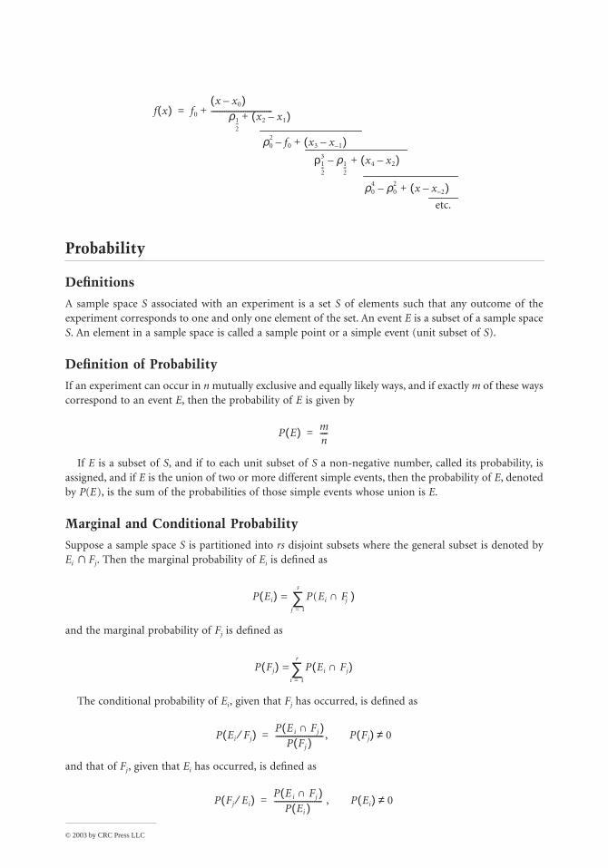
© 2003 by CRC Press LLC
Probability
Definitions
A sample space S associated with an experiment is a set S of elements such that any outcome of the experiment corresponds to one and only one element of the set. An event E is a subset of a sample space S. An element in a sample space is called a sample point or a simple event (unit subset of S).
Definition of Probability
If an experiment can occur in n mutually exclusive and equally likely ways, and if exactly m of these ways correspond to an event E, then the probability of E is given by
If E is a subset of S, and if to each unit subset of S a non-negative number, called its probability, is assigned, and if E is the union of two or more different simple events, then the probability of E, denoted by P(E ), is the sum of the probabilities of those simple events whose union is E.
Marginal and Conditional Probability
Suppose a sample space S is partitioned into rs disjoint subsets where the general subset is denoted by Ei ∩ Fj . Then the marginal probability of Ei is defined as
and the marginal probability of Fj is defined as
The conditional probability of Ei , given that Fj has occurred, is defined as
and that of Fj , given that Ei has occurred, is defined as
f x( ) f0
x x0–( )ρ1
2--
x2 x1–( )+--------------------------------+=
ρ02 f0– x3 x 1––( )+
ρ12--
3 ρ12--
– x4 x2–( )+
ρ04 ρ0
2 – x x 2––( )+
etc.
P E( ) mn----=
P Ei( ) = P(Ei Fj )∩j 1=
s
∑
P Fj( ) = P Ei Fj∩( )i 1=
r
∑
P Ei Fj⁄( ) P E( i Fj )∩P Fj )(
------------------------- , P Fj( ) 0≠=
P Fj Ei⁄( ) P E( i Fj )∩P Ei )(
------------------------- , P Ei( ) 0≠=
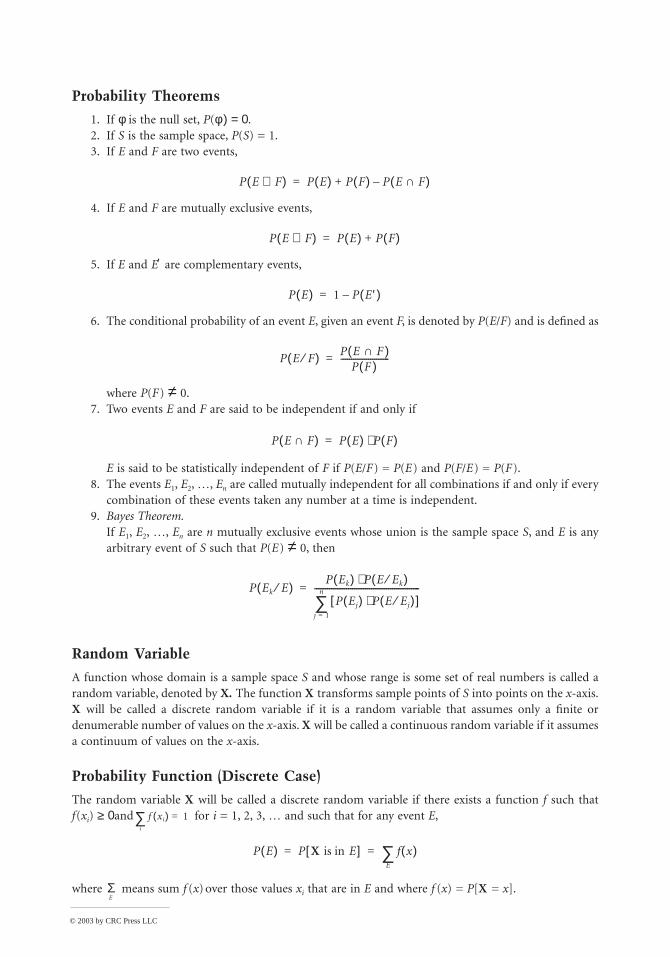
© 2003 by CRC Press LLC
Probability Theorems
1. If φ is the null set, P(φ ) = 0.2. If S is the sample space, P(S) = 1.3. If E and F are two events,
4. If E and F are mutually exclusive events,
5. If E and E′ are complementary events,
6. The conditional probability of an event E, given an event F, is denoted by P(E/F) and is defined as
where P(F ) ≠ 0.7. Two events E and F are said to be independent if and only if
E is said to be statistically independent of F if P(E/F ) = P(E ) and P(F/E ) = P(F ).8. The events E1, E2, K, En are called mutually independent for all combinations if and only if every
combination of these events taken any number at a time is independent.9. Bayes Theorem.
If E1, E2, K, En are n mutually exclusive events whose union is the sample space S, and E is any arbitrary event of S such that P(E ) ≠ 0, then
Random Variable
A function whose domain is a sample space S and whose range is some set of real numbers is called a random variable, denoted by X. The function X transforms sample points of S into points on the x-axis. X will be called a discrete random variable if it is a random variable that assumes only a finite or denumerable number of values on the x-axis. X will be called a continuous random variable if it assumes a continuum of values on the x-axis.
Probability Function (Discrete Case)
The random variable X will be called a discrete random variable if there exists a function f such that f (xi) ≥ 0 and for i = 1, 2, 3, K and such that for any event E,
where means sum f (x) over those values xi that are in E and where f (x) = P[X = x].
P E F∪( ) P E( ) P F( ) P E F∩( )–+=
P E F∪( ) P E( ) P F( )+=
P E( ) 1 P E ′( )–=
P E F⁄( ) P E( F )∩P F )(
-----------------------=
P E F∩( ) P E( ) P F( )⋅=
P Ek E⁄( )P Ek( ) P E Ek⁄( )⋅
P Ej( ) P E Ej⁄( )⋅[ ]j 1=
n
∑--------------------------------------------------=
f xi( )i
∑ 1=
P E( ) P X is in E[ ] f x( )E∑= =
ΣE
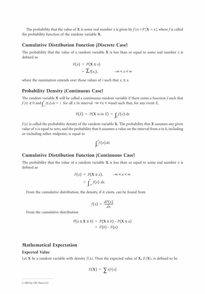
© 2003 by CRC Press LLC
The probability that the value of X is some real number x is given by f (x) = P [X = x], where f is called the probability function of the random variable X.
Cumulative Distribution Function (Discrete Case)
The probability that the value of a random variable X is less than or equal to some real number x is defined as
where the summation extends over those values of i such that xi ≤ x.
Probability Density (Continuous Case)
The random variable X will be called a continuous random variable if there exists a function f such that f (x) ≥ 0 and for all x in interval −∞ < x < ∞ and such that, for any event E,
f (x) is called the probability density of the random variable X. The probability that X assumes any given value of x is equal to zero, and the probability that it assumes a value on the interval from a to b, including or excluding either endpoint, is equal to
Cumulative Distribution Function (Continuous Case)
The probability that the value of a random variable X is less than or equal to some real number x is defined as
From the cumulative distribution, the density, if it exists, can be found from
From the cumulative distribution
Mathematical Expectation
Expected Value
Let X be a random variable with density f (x). Then the expected value of X, E (X), is defined to be
F x( ) P X x≤( )=
Σ f xi( ), ∞– x ∞< <=
f x( ) xd∞–
∞
∫ 1=
P E( ) P X is in E( ) f x( ) xdE∫= =
f x( ) xda
b
∫
F x( ) P X x≤( ), ∞– x ∞< <=
f x( ) x.d∞–
∞
∫=
f x( ) dF x( )dx
--------------=
P a X b≤ ≤( ) P X b≤( ) P X a≤( )–=
F b( ) F a( )–=
E X( ) xf x( )x∑=

© 2003 by CRC Press LLC
if X is discrete and
if X is continuous. The expected value of a function g of a random variable X is defined as
if X is discrete and
if X is continuous.
Positional Notation
In our ordinary system of writing numbers, the value of any digit depends on its position in the number. The value of a digit in any position is ten times the value of the same digit one position to the right, or one-tenth the value of the same digit one position to the left. Thus, for example,
There is no reason that a number other than 10 cannot be used as the base, or radix, of the number system. In fact, bases of 2, 8, and 16 are commonly used in working with digital computers. When the base used is not clear from the context, it is usually indicated as a parenthesized subscript or merely as a subscript. Thus,
Change of Base
In this section, it is assumed that all calculations will be performed in base 10, since this is the only base in which most people can easily compute. However, there is no logical reason that some other base could not be used for the computations.
To convert a number from another base into base 10:Simply write down the digits of the number, with each one multiplied by its appropriate positional
value. Then perform the indicated computations in base 10, and write down the answer.For examples, see the two examples in the previous section.To convert a number from base 10 into another base:The part of the number to the left of the point and the part to the right must be operated on separately.
For the integer part (the part to the left of the point):
a. Divide the number by the new base, getting an integer quotient and remainder.b. Write down the remainder as the last digit of the number in the new base.c. Using the quotient from the last division in place of the original number, repeat the above two
steps until the quotient becomes zero.
E X( ) xf x( ) xd∞–
∞
∫=
E g X( )[ ] g x( ) f x( )⋅x∑=
E g X( )[ ] g x( ) f x( )⋅ xd∞–
∞
∫=
173.246 1 102 7 101×+× 3 2 110-----× 4 1
102-------× 6 1
103-------×+ + + +=
743 8( ) 7 82× 4 8 3 7 64 4 8 3+×+×=+×+ 448 32 3 483 10( )=+ += =
1011.101 2( ) 1 23 0 22 1 2 1 1 12---×+ +×+×+× 0 1
4---× 1 1
8---× 11.625 10( )=+ +=
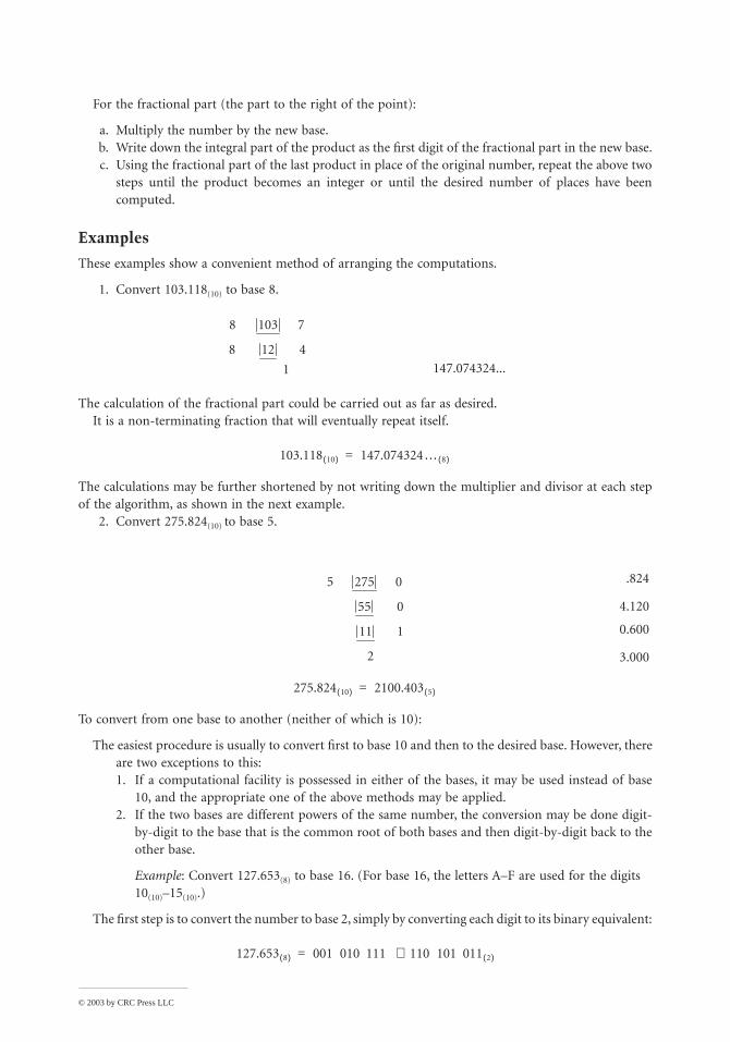
© 2003 by CRC Press LLC
For the fractional part (the part to the right of the point):
a. Multiply the number by the new base.b. Write down the integral part of the product as the first digit of the fractional part in the new base.c. Using the fractional part of the last product in place of the original number, repeat the above two
steps until the product becomes an integer or until the desired number of places have been computed.
Examples
These examples show a convenient method of arranging the computations.
1. Convert 103.118(10) to base 8.
The calculation of the fractional part could be carried out as far as desired.It is a non-terminating fraction that will eventually repeat itself.
The calculations may be further shortened by not writing down the multiplier and divisor at each step of the algorithm, as shown in the next example.
2. Convert 275.824(10) to base 5.
To convert from one base to another (neither of which is 10):
The easiest procedure is usually to convert first to base 10 and then to the desired base. However, there are two exceptions to this:1. If a computational facility is possessed in either of the bases, it may be used instead of base
10, and the appropriate one of the above methods may be applied.2. If the two bases are different powers of the same number, the conversion may be done digit-
by-digit to the base that is the common root of both bases and then digit-by-digit back to the other base.
Example: Convert 127.653(8) to base 16. (For base 16, the letters A–F are used for the digits 10(10)–15(10).)
The first step is to convert the number to base 2, simply by converting each digit to its binary equivalent:
8 103 7
8 12 4
1 147.074324...
103.118 10( ) 147.074324… 8( )=
5 275 0
55 0
11 1
2
.824
4.120
0.600
3.000
275.824 10( ) 2100.403 5( )=
127.653 8( ) 001 010 111 110 101 011 2( )⋅=
© 2003 by CRC Press LLC
Now by simply regrouping the binary number into groups of four binary digits, starting at the point, we convert to base 16:
Credits
Material in this section was reprinted from the following sources:
D.R. Lide, Ed., CRC Handbook of Chemistry and Physics, 73rd ed., Boca Raton, FL: CRC Press. 1992: International System of Units (SI), conversion constants and multipliers (conversion of temperatures), symbols and terminology for physical and chemical quantities, fundamental physical constants.
W.H. Beyer, Ed., CRC Standard Mathematical Tables and Formulae, 29th ed., Boca Raton, FL: CRC Press, 1991: Greek alphabet, conversion constants and multipliers (recommended decimal multiples and submultiples, metric to English, English to metric, general, temperature factors), physical constants, series expansion, integrals, the Fourier transforms, numerical methods, probability, positional notation.
R.J. Tallarida, Pocket Book of Integrals and Mathematical Formulas, 2nd ed., Boca Raton, FL: CRC Press, 1992: Elementary algebra and geometry; determinants, matrices, and linear systems of equations; trigonometry; analytic geometry; series; differential calculus; integral calculus; vector analysis; special functions; statistics; tables of probability and statistics; table of derivatives.
Associations and Societies
American Concrete Institute (ACI)PO Box 9094Farmington Hills, MI 48333Tel. # (248) 848-3700Homepage: http://www.aci-int.net/
Founded in 1905, the American Concrete Institute (ACI) has grown into a chartered society with over 20,000 members worldwide. The ACI is a technical and educational nonprofit society dedicated to improving the design, construction, manufacture, and maintenance of concrete structures.
Among ACI’s 20,000 members are structural designers, architects, civil engineers, educators, contrac-tors, concrete craftsmen and technicians, representatives of materials suppliers, students, testing labora-tories, and manufacturers from around the world. The 83 national and international chapters provide the membership with opportunities to network with their peers and keep in tune with the activities of ACI International.
Membership
Membership is open to individuals who work directly in, have an association with, or have an interest in concrete. All members are encouraged to participate in the activities of the ACI International, which include involvement on voluntary technical committees that develop ACI codes, standards, and reports. Various levels of membership exist to meet particular needs. Student memberships are available.
Publications
Concrete International. Published monthly. Covers institute, chapter, and industry news. Several technical articles following a specific theme appear in each issue.
ACI Materials Journal. Published bimonthly. Describes research in materials and concrete, related ACI International standards, and committee reports.
127.653 8( ) 101 0111 1101 0101 1 2( )⋅ 57.D58 16( )= =

© 2003 by CRC Press LLC
ACI Structural Journal. Published bimonthly. Includes technical papers on structural design and analysis, state-of-the-art reviews on reinforced and structural elements, and the use and handling of concrete.
Other publications: ACI International makes available over 300 technical publication on concrete. Infor-mation is also available in computer software and compact disc formats. A free 72-page publications catalog describing what ACI International has to offer is available.
Other Activities
ACI International provides technical information in the form of high-quality conventions, seminars, and symposia.
American Iron and Steel Institute (AISI)1101 17th Street NW, Suite 1300Washington, DC 20036Tel. (202) 452-7100Homepage: http://www.steel.org/
The American Iron and Steel Institute (AISI) was founded in 1908. The institute is a nonprofit association of North American companies engaged in the iron and steel industry. AISI comprises 43 member companies that produce the full range of steel mill products. Also included are iron ore mining companies and member companies that produce raw steel, including integrated, electric furnace, and reconstituted mills. Member companies account for more than two-thirds of the raw steel produced in the U.S., most of the steel manufactured in Canada, and nearly two-thirds of the flat-rolled steel products manufactured in Mexico.
AISI has 230 associate members, including customers who distribute, fabricate, process, or consume steel. Also included are companies and representatives of organizations that supply the steel industry with materials, equipment, and services, as well as individuals associated with educational or research organizations.
American National Standards Institute (ANSI)Washington, DC, Headquarters1819 L Street NW, 6th Fl.Washington, DC 20036Tel. (202) 293-8020Fax. (202) 293-9287
New York City Office25 West 43rd Street, 4th FloorNew York, NY, 10036Tel. (212) 642-4900Fax. (212) 398-0023Homepage: http://www.ansi.org/ E-mail: [email protected]
Founded in 1918, the American National Standards Institute (ANSI) is a private, nonprofit membership organization that coordinates the U.S. voluntary consensus standards system and approves American National Standards. ANSI ensures that a single set of nonconflicting American National Standards are developed by ANSI-accredited standards developers and that all interests concerned have the opportunity to participate in the development process.
ANSI is the official U.S. representative to the International Accreditation Forum (IAF), the Interna-tional Organization for Standardization (ISO), and, via the U.S. National Committee, the International Electrotechnical Commission (IEC). ANSI is also the U.S. member of the Pacific Area Standards Congress (PASC) and the Pan American Standards Commission (COPANT).

© 2003 by CRC Press LLC
Membership
ANSI consists of approximately 1300 national and international companies, 30 government agencies, 20 institutional members, and 250 professional, technical, trade, labor, and consumer organizations. ANSI offers no individual membership. For more information on membership, write to the Member Services Department at the New York Office; call (212) 642-4900; or e-mail [email protected].
Publications
ANSI Reporter. Published monthly. Newsletter that updates members on major national and international standards activities. It also provides information on the activities of the European standards bodies, CEN and CENELEC.
Standards Action. Published biweekly. This newsletter outlines all national draft standards currently under consideration for approval as American National Standards and solicits comments from readers. Com-ments are also solicited on regional, international, and foreign standards. These comments are then reviewed as part of the development process.
Catalog of American National Standards. Published annually. Provides a complete listing of all ANSI-approved American National Standards. Supplements are also published.
American Railway Engineering and Maintenance-of-Way Association (AREMA)8201 Corporate Drive, Suite 1125Landover, MD 20785Tel. (301) 459-3200Fax. (301) 459-8077Homepage: http://www.arema.org
The American Railway Engineering and Maintenance-of-Way Association (AREMA) was formed on October 1, 1997, as the result of a merger of three engineering support associations, namely the American Railway Bridge and Building Association, the American Railway Engineering Association, and the Road-masters and Maintenance of Way Association, along with functions of the Communications and Signal Division of the Association of American Railroads. The rich history of the predecessor organizations, each having over 100 years of service to the rail industry, is the legacy of AREMA.
Each of the four groups — Roadmasters and Maintenance of Way Association, American Railway Bridge and Building Association, American Railway Engineering Association, and Communications and Signal Division — that came together to form AREMA have, in their own way, built an excellent foundation upon which to base the new association, whose mission is the development and advancement of both technical and practical knowledge and recommended practices pertaining to the design, con-struction, and maintenance of railway infrastructure.
Membership
The basic qualifications for membership are five years of experience in the profession of maintaining, operating, constructing, or locating railways. Graduation from a recognized college or university with a degree in engineering is being taken as the equivalent of three years of experience.
Publications
AREMA Manual for Railway Engineering comprises the work of the association’s committees. The manual is revised annually to make the latest in recommended practice information for railway engineering available to all interested parties. The Portfolio of Trackwork Plans is also compiled and updated in the same manner.
American Society of Civil Engineers (ASCE)International Headquarters1801 Alexander Bell DriveReston, VA 20191-4400
© 2003 by CRC Press LLC
Tel. 1-800-548-2723 (toll-free) / (703) 295-6300Fax. (703) 295-6222 / (703) 295-6444 (fax-back)
Washington Office1015 15th Street NW, Suite 600Washington, DC 20005Tel. (202) 789-2200Fax. (202) 289-6797
Founded in 1852, the American Society of Civil Engineers (ASCE) is America's oldest national profes-sional engineering society. The society has more than 115,000 individual members, including 6,500 international members in 137 nations. Memberships consist of individual professional engineers rather than companies or organizations.
ASCE is organized geographically into 21 district councils, 83 sections, 143 branches, and 246 student chapters and clubs. The society is governed by a 28-member board and is headquartered in the United Engineering Center in New York City. A Washington, DC, office is maintained for government relations.
ASCE maintains the Civil Engineering Research Foundation to focus national attention and resources on the research needs of the civil engineering profession. In addition, there are 25 technical divisions and councils that foster the development and advancement of the science and practice of engineering. ASCE has marked infrastructure renewal as a top national priority.
ASCE is the world’s largest publisher of civil engineering information, publishing over 63,000 pages in 1994. Nearly 42% of the society's yearly income is generated through publication sales.
Membership
Membership applicants must meet the requirements set in the constitution of the ASCE. Various levels of membership exist to meet particular needs. Student memberships are available to students who meet the requirements of the constitution. Various entrance fees and dues are required of the various levels of membership. Application materials may be requested by mailing the ASCE Membership Services Department, phoning 800-548-2723 (toll-free in the United States) or 703-295-6300 (internationally), faxing 703-295-6333, or e-mailing your request to [email protected].
Publications
Civil Engineering. Published monthly. This is the society’s official magazine and is mailed to all members of ASCE. The magazine contains articles of current interest in the various fields of civil engineering, news of a professional nature, and reports on the activities of ASCE and its members. Independently prepared papers may be sent directly to the editor of Civil Engineering at 345 East 47th Street, New York, NY 10017-2398.
ASCE News. Published monthly. Mailed to all members without charge. It concentrates on the activities of ASCE and its members, with the intent of promoting interest and participation in society programs.
Worldwide Projects. Published quarterly. A copublication of ASCE and Intercontinental Media, Inc., Westport, CT. Each issue provides engineers with articles giving insight into various topics related to international civil engineering projects and doing business outside the U.S.
Journals published: Journal of Management in Engineering, published bimonthly, and Journal of Profes-sional Issues in Engineering Education and Practice, published quarterly, present professional and technical problems of broad interest and implications. ASCE also publishes significant reports of the Professional Activities Committee and its constituent committees.
Other publications: The society also publishes transactions; standards; engineer-, owner-, and construc-tion-related documents; the publications information and indexes; and newsletters. A civil engineering database is also available. For inquiries on prices or to request a catalog or sample issues, e-mail [email protected]; phone 1-800-548-2723, ext. 6251 (U.S.), or 703-295-6163 (international); fax 703-295-6278; or mail American Society of Civil Engineers, Publications Marketing Department, 1801 Alex-ander Bell Drive, Reston, VA 20191-4400.

© 2003 by CRC Press LLC
American Society for Testing and Materials (ASTM)International Headquarters100 Barr Harbor DriveWest Conshohocken, PA 19428-2959Tel. (610) 832-9500Fax (610) 832-9555Homepage: http://www.astm.org/
Founded in 1898, the American Society for Testing and Materials (ASTM) has grown into one of the largest voluntary standards development systems in the world. ASTM is a nonprofit organization that provides a forum for producers, users, ultimate consumers, and those having a general interest, such as representatives of government and academia, to meet on common ground and write standards for materials, products, systems, and services. From the work of 131 standard-writing committees, ASTM publishes standard test methods, specifications, practices, guides, classifications, and terminology. ASTM’s standards development activities encompass metals, paints, plastics, textiles, petroleum, con-struction, energy, the environment, consumer products, medical services and devices, computerized systems, electronics, and many other areas. All technical research and testing are done voluntarily by more than 35,000 technically qualified ASTM members located throughout the world.
Membership
ASTM members pay an annual administrative fee of $75 for individual membership and $400 for an organizational membership. The only other costs involved are the time and travel expenses of the committee members and the donated use of members’ laboratory and research facilities.
Publications
Annual Book of ASTM Standards. A 70-volume set that includes standards and specs in the following subject areas:
Iron and steel products Nonferrous metal products Metals test methods and analytical proceduresConstruction Petroleum products, lubricants, and fossil fuels Medical devices and services General methods and instrumentationPaints, related coatings, and aromaticsTextilesPlastics Rubber Electrical insulation and electronics Water and environmental technologyNuclear, solar, and geothermal energy General products, chemical specialties, and end-use products
Discounts are applied when purchased as a complete set or when purchased by complete sections. Volumes may also be purchased individually.
Standardization News. Published monthly.
Journals published: Journal of Testing and Evaluation; Cement, Concrete, and Aggregates; Geotechnical Testing Journal, Journal of Composites Technology and Research; and Journal of Forensic Sciences.
ASTM also publishes books containing reports on state-of-the-art testing techniques and their possible applications.

© 2003 by CRC Press LLC
American Water Works AssociationHeadquarters6666 West Quincy AvenueDenver, CO 80235 Tel. (303) 794-7711Fax. (303) 794-7310
Government Affairs Office 1401 New York Avenue NW, Suite 640 Washington, DC 20005 Tel. (202) 628-8303Fax. (202) 628-2846 Homepage: http://www.awwa.org/
The American Water Works Association (AWWA) was established in 1881 by 22 dedicated water supply professionals. Membership has grown to more than 54,000 individuals and organizations. AWWA is an international, nonprofit, scientific, and educational association dedicated to improving drinking water for people everywhere. Today, AWWA has grown to be the largest organization of water supply profes-sionals in the world, boasting members from virtually every country.
AWWA was formed to promote public health, safety, and welfare through the improvement of the quality and quantity of water delivered to the public and through the development of public understand-ing. AWWA also takes an active role in shaping the water industry’s direction through research, partici-pation in legislative activities, development of products, procedural standards, and manuals of practice, and it educates the public on water issues to promote a spirit of cooperation between consumers and buyers.
Membership
Listed under individual memberships are active, affiliate, and student. Organization memberships include utility, municipal service subscriber, small water system, associate, consultant, contractor, technical ser-vice, and manufacturer’s agent, distributor, or representative. The association is governed by a board of directors that establishes policy for the overall management and direction of association affairs.
Publications
AWWA is the world’s major publisher of drinking water information. Its publications cover just about every area of interest in the water supply field. More than 500 titles are offered, covering all aspects of water resources, water quality, treatment and distribution, utility management, and employee training and safety.
Civil Engineering Research Foundation (CERF)2131 K Street NW, Suite 700Washington, DC 20037Tel. (202) 785-6420Fax. (202) 833-2604Homepage: http://www.cerf.org/
The Civil Engineering Research Foundation (CERF) was created by the American Society of Civil Engi-neers and began operation in 1989 to advance the civil engineering profession through research. CERF is an industry-guided research organization that serves as a critical catalyst to help the design and construction industry and the civil engineering profession expedite the transfer of research results into practice through cooperative national programs. CERF integrates the efforts of industry, government, and academia in order to implement research that is beyond the capabilities of any single organization. CERF is an independent, nonprofit organization but remains affiliated with ASCE.

© 2003 by CRC Press LLC
Council on Tall Buildings and Urban Habitat Lehigh University 117 ATLSS DriveBethlehem, PA 18015 Tel. (215) 758-3515Fax (215) 758-4522 Homepage: http://www.lehigh.edu/~inctbuh/ E-mail: [email protected]
The Council on Tall Buildings and Urban Habitat is an international organization sponsored by engi-neering, architectural, and planning professionals. The council was founded in 1969 and was known as the Joint Committee on Tall Buildings until the name was changed in 1976 to its present form.
The council was established to study and report on all aspects of the planning, design, construction, and operation of tall buildings. The council is also concerned with the role of tall buildings in the urban environment and their impact thereon. However, the council is not an advocate for tall buildings per se, but in those situations in which they are viable, the council seeks to encourage the use of the latest knowledge in their implementation.
Membership
Membership is available to associations, commercial organizations, individual members, and students. Membership is available to students at the rate of $10 per year. Membership fees vary for associations, commercial organizations, and individuals.
Publications
A major focus of the council is the publication of a comprehensive monograph series for use by those responsible for tall building planning and design. The original five-volume Monograph on the Planning and Design of Tall Buildings was released between 1978 and 1981. This comprehensive source of tall building information is the only such reference tool now available to the high-rise specialist. The volumes are Planning and Environmental Criteria for Tall Buildings, Tall Building Systems and Concepts, Tall Building Criteria and Loading, Structural Design of Tall Street Buildings, and Structural Design of Tall Concrete and Masonry Buildings. These volumes are available as a set or sold separately. Updated monographs are continually added to the series in order to keep information current.
Structural Stability Research CouncilHeadquartersUniversity of FloridaDepartment of Civil and Coastal Engineering345 Weil Hall, PO Box 116580Gainesville, FL 32611-6580Tel. (352) 846-3874, ext. 1424Fax. (352) 846-3978Homepage: http://www.ce.ufl.edu/~ssrc/ Email: [email protected]
The Structural Stability Research Council (formerly the Column Research Council) was founded in 1944 to review and resolve the conflicting opinions and practices that existed at the time with respect to solutions to stability problems and to facilitate and promote economical and safe design. Now, more than 50 years later, the council has broadened its scope within the field of structural stability, has become international in character, and continues to seek solutions to stability problems.
© 2003 by CRC Press LLC
Membership
Various levels of membership exist for individuals. Organizations, companies, and firms concerned with investigation and design of metal and composite structures are invited by the council to become sponsors, participating organizations, participating companies, or participating firms.
Publications
The council maintains a library at its headquarters. Material from the library is available on request.
Transportation Research Board (TRB) Cecil and Ida Green Building 2001 Wisconsin Avenue NWWashington, DC 20007 Tel. (202) 334-2934Fax (202) 334-2003 Homepage: http://www.nas.edu/trb/
The Transportation Research Board (TRB) is a unit of the National Research Council, which serves the National Academy of Sciences and the National Academy of Engineering. The board’s purpose is to stimulate research concerning the nature and performance of transportation systems, to disseminate the information produced by the research, and to encourage the application of appropriate research findings. The board’s program is carried out by more than 330 committees, task forces, and panels composed of more than 3900 administrators, engineers, social scientists, attorneys, educators, and others concerned with transportation; they serve without compensation.
The program is supported by state transportation and highway departments, modal administrations of the U.S. Department of Transportation, and others interested in the development of transportation.
In November 1920, after a series of preliminary meetings and conferences, the National Research Council created the Advisory Board on Highway Research. Four years later, the name was changed to the Highway Research Board. During the late 1960s, the Highway Research Board expanded its scope to all modes of transportation. The name was again changed in 1974 to the Transportation Research Board to recognize its increased emphasis on a broadened approach to transportation problems and needs.
Today the Transportation Research Board devotes attention to all factors pertinent to the understand-ing, design, and function of systems for the safe and efficient movement of people and goods, including the following:
• Planning, design, construction, operation, safety, and maintenance of transportation facilities and their components
• Economics, financing, and administration of transportation facilities and services
• Interaction of transportation systems with one another and with the physical, economic, and social environment that they are designed to serve
Publications
One of the most important activities of the Transportation Research Board is the dissemination of current research results. The mainstay of the TRB publications program is the Transportation Research Record series. This series consists primarily of the papers delivered at the TRB annual meeting by authors from all over the world.
Ethics
The following code of ethics was adopted by the American Society of Civil Engineers on September 25, 1976. The code of ethics became effective on January 1, 1977. The ASCE has since amended this code on October 25, 1980, and April 17, 1993. The code of ethics shown below is in the most recent amended form.

© 2003 by CRC Press LLC
The ASCE adopted the fundamental principles of the ABET Code of Ethics of Engineers as accepted by the Accreditation Board for Engineering and Technology, Inc. (ABET).
Code of Ethics1
Fundamental Principles
Engineers uphold and advance the integrity, honor and dignity of the engineering profession by:
1. using their knowledge and skill for the enhancement of human welfare;2. being honest and impartial and serving with fidelity the public, their employers and clients;3. striving to increase the competence and prestige of the engineering profession; and4. supporting the professional and technical societies of their disciplines.
Fundamental Canons
1. Engineers shall hold paramount the safety, health and welfare of the public in the performance of their professional duties.
2. Engineers shall perform services only in areas of their competence.3. Engineers shall issue public statements only in an objective and truthful manner.4. Engineers shall act in professional matters for each employer or client as faithful agents or trustees,
and shall avoid conflicts of interest.5. Engineers shall build their professional reputation on the merit of their services and shall not
compete unfairly with others.6. Engineers shall act in such a manner as to uphold and enhance the honor, integrity and dignity
of the engineering profession.7. Engineers shall continue their professional development throughout their careers, and shall pro-
vide opportunities for the professional development of those engineers under their supervision.
Guidelines to Practice Under the Fundamental Canons of Ethics
CANON 1. Engineers shall hold paramount the safety, health and welfare of the public in the perfor-mance of their professional duties.
a. Engineers shall recognize that the lives, safety, health and welfare of the general public are depen-dent upon engineering judgments, decisions and practices incorporated into structures, machines, products, processes and devices.
b. Engineers shall approve or seal only those design documents, reviewed or prepared by them, which are determined to be safe for public health and welfare in conformity with accepted engineering standards.
c. Engineers whose professional judgment is overruled under circumstances where the safety, health and welfare of the public are endangered, shall inform their clients or employers of the possible consequences.
d. Engineers who have knowledge or reason to believe that another person or firm may be in violation of any of the provisions of Canon 1 shall present such information to the proper authority in writing and shall cooperate with the proper authority in furnishing such further information or assistance as may be required.
e. Engineers should seek opportunities to be of constructive service in civic affairs and work for the advancement of the safety, health and well-being of their communities.
f. Engineers should be committed to improving the environment to enhance the quality of life.
1Published with permission of the American Society of Civil Engineers.

© 2003 by CRC Press LLC
CANON 2. Engineers shall perform services only in areas of their competence.
a. Engineers shall undertake to perform engineering assignments only when qualified by education or experience in the technical field of engineering involved.
b. Engineers may accept an assignment requiring education or experience outside of their own fields of competence, provided their services are restricted to those phases of the project in which they are qualified. All other phases of such project shall be performed by qualified associates, consultants or employees.
c. Engineers shall not affix their signatures or seals to any engineering plan or document dealing with subject matter in which they lack competence by virtue of education or experience or to any such plan or document not reviewed or prepared under their supervisory control.
CANON 3. Engineers shall issue public statements only in an objective and truthful manner.
a. Engineers should endeavor to extend the public knowledge of engineering, and shall not participate in the dissemination of untrue, unfair or exaggerated statements regarding engineering.
b. Engineers shall be objective and truthful in professional reports, statements or testimony. They shall include all relevant and pertinent information in such reports, statements or testimony.
c. Engineers, when serving as expert witnesses, shall express an engineering opinion only when it is founded upon adequate knowledge of the facts, upon a background of technical competence and upon honest conviction.
d. Engineers shall issue no statements, criticisms or arguments on engineering matters which are inspired or paid for by interested parties, unless they indicate on whose behalf the statements are made.
e. Engineers shall be dignified and modest in explaining their work and merit, and will avoid any act tending to promote their own interests at the expense of the integrity, honor and dignity of the profession.
CANON 4. Engineers shall act in professional matters for each employer or client as faithful agents or trustees, and shall avoid conflicts of interest.
a. Engineers shall avoid all known or potential conflicts of interest with their employers or clients and shall promptly inform their employers or clients of any business association, interests or circumstances which could influence their judgment or the quality of their services.
b. Engineers shall not accept compensation from more than one party for services on the same project, or for services pertaining to the same project, unless the circumstances are fully disclosed to and agreed to by all interested parties.
c. Engineers shall not solicit or accept gratuities, directly or indirectly, from contractors, their agents or other parties dealing with their clients or employers in connection with work for which they are responsible.
d. Engineers in public service as members, advisors or employees of a governmental body or depart-ment shall not participate in considerations or actions with respect to services solicited or provided by them or their organization in private or public engineering practice.
e. Engineers shall advise their employers or clients when, as a result of their studies, they believe a project will not be successful.
f. Engineers shall not use confidential information coming to them in the course of their assignments as a means of making personal profit if such action is adverse to the interests of their clients, employers or the public.
g. Engineers shall not accept professional employment outside of their regular work or interest without the knowledge of their employers.

© 2003 by CRC Press LLC
CANON 5. Engineers shall build their professional reputation on the merit of their services and shall not compete unfairly with others.
a. Engineers shall not give, solicit or receive either directly or indirectly, any political contribution, gratuity or unlawful consideration in order to secure work, exclusive of securing salaried positions through employment agencies.
b. Engineers should negotiate contracts for professional services fairly and on the basis of demon-strated competence and qualifications for the type of professional service required.
c. Engineers may request, propose or accept professional commissions on a contingent basis only under circumstances in which their professional judgments would not be compromised.
d. Engineers shall not falsify or permit misrepresentation of their academic or professional qualifi-cations or experience.
e. Engineers shall give proper credit for engineering work to those to whom credit is due, and shall recognize the proprietary interests of others. Whenever possible, they shall name the person or persons who may be responsible for designs, inventions, writings or other accomplishments.
f. Engineers may advertise professional services in a way that does not contain misleading language or is in any other manner derogatory to the dignity of the profession. Examples of permissible advertising are as follows:
Professional cards in recognized, dignified publications, and listings in rosters or directories published by responsible organizations, provided that the cards or listings are consistent in size and content and are in a section of the publication regularly devoted to such professional cards.
Brochures which factually describe experience, facilities, personnel and capacity to render service, providing they are not misleading with respect to the engineer’s participation in projects described.
Display advertising in recognized dignified business and professional publications, providing it is factual and is not misleading with respect to the engineer’s extent of participation in projects described.
A statement of the engineers’ names or the name of the firm and statement of the type of service posted on projects for which they render services.
Preparation or authorization of descriptive articles for the lay or technical press, which are factual and dignified. Such articles shall not imply anything more than direct participation in the project described.
Permission by engineers for their names to be used in commercial advertisements, such as may be published by contractors, material suppliers, etc., only by means of a modest, dignified notation acknowledging the engineers’ participation in the project described. Such per-mission shall not include public endorsement of proprietary products.
g. Engineers shall not maliciously or falsely, directly or indirectly, injure the professional reputation, prospects, practice or employment of another engineer or indiscriminately criticize another’s work.
h. Engineers shall not use equipment, supplies, laboratory or office facilities of their employers to carry on outside private practice without the consent of their employers.
CANON 6. Engineers shall act in such a manner as to uphold and enhance the honor, integrity and dignity of the engineering profession.
a. Engineers shall not knowingly act in a manner which will be derogatory to the honor, integrity or dignity of the engineering profession or knowingly engage in business or professional practices of a fraudulent, dishonest or unethical nature.

© 2003 by CRC Press LLC
CANON 7. Engineers shall continue their professional development throughout their careers, and shall provide opportunities for the professional development of those engineers under their supervision.
a. Engineers should keep current in their specialty fields by engaging in professional practice, par-ticipating in continuing education courses, reading in the technical literature and attending pro-fessional meetings and seminars.
b. Engineers should encourage their engineering employees to become registered at the earliest possible date.
c. Engineers should encourage engineering employees to attend and present papers at professional and technical society meetings.
d. Engineers shall uphold the principle of mutually satisfying relationships between employers and employees with respect to terms of employment, including professional grade descriptions, salary ranges and fringe benefits.