APPENDIX G HYDRAULIC GRADE LINE 1.0 … · April 2014 ODOT Hydraulics Manual . 13-G-2 Storm...

Storm Drainage 13-G-1

APPENDIX G HYDRAULIC GRADE LINE

1.0 Introduction

The hydraulic grade line is used to aid the designer in determining the acceptability of a proposed or evaluation of an existing storm drainage system by establishing the elevation to which water will rise when the system is operating under design conditions. Detail on this system performance analysis is presented in this appendix. 2.0 Definitions

Definitions of terms which will be important in a storm drainage analysis and design are provided in this section. These and other terms defined in the manual glossary will be used throughout the remainder of this appendix in dealing with different aspects of storm drainage analysis. Energy grade line – Represents the total available energy in the system (potential energy plus kinetic energy). Hydraulic grade line - The hydraulic grade line (HGL), a measure of flow energy, is a line coinciding with the level of flowing water at any point along an open channel. In closed conduits flowing under pressure, the hydraulic grade line is the level to which water would rise in a vertical tube (open to atmospheric pressure) at any point along the pipe. HGL is determined by subtracting the velocity head (V2/2g) from the energy gradient (or energy grade line). Figure 1 illustrates the energy and hydraulic grade lines for open channel and pressure flow in pipes. As illustrated in Figure 1, if the HGL is above the inside top (crown) of the pipe, pressure flow conditions exist. Conversely, if the HGL is below the crown of the pipe, open channel flow conditions exist. Critical depth – is defined as the depth for which the specific energy (sum of the flow depth and velocity head) of a given discharge is at a minimum. A slight change in specific energy can result in a significant rise or fall in the water depth when flow is at or near critical depth. Because of this, critical depth is an unstable condition and it rarely occurs for any distance along a water surface profile.

April 2014 ODOT Hydraulics Manual

13-G-2 Storm Drainage

Figure 1 - Hydraulic and Energy Grade Lines in Pipe Flow 3.0 Design Guidelines

Storm drainage systems operating under surcharge conditions (pressure flow) shall evaluate the hydraulic grade line and minor losses such as manhole losses, bends in pipes, expansion and contraction losses, etc. Adjust inlet sizes/locations and pipe sizes/location to correct hydraulic grade line problems. Pressure flow design must assure the hydraulic grade line is 0.5 feet or more below rim elevation of any drainage structure which may be affected. The energy grade line must also be at or below the rim elevation of any drainage structure which may be affected.

ODOT Hydraulics Manual April 2014


4.0 Tailwater

Evaluation of the hydraulic grade line for a storm drainage system begins at the system outfall with the tailwater elevation. For most design applications, the tailwater will either be above the crown of the outlet or can be considered to be between the crown and critical depth of the outlet. The tailwater may also occur between the critical depth and the invert of the outlet, however, the starting point for the hydraulic grade line determination should be either the design tailwater elevation or (dc + D)/2, whichever is highest, where dc is outlet critical depth and D is crown depth. An exception to the above rule would be for a very large outfall with low tailwater where a water surface profile calculation would be appropriate to determine the location where the water surface will intersect the top of the barrel and full flow calculations can begin. In this case, the downstream water surface elevation would be based on critical depth or the design tailwater elevation, whichever was highest. If the outfall channel is a river or stream, it may be necessary to consider the joint or coincidental probability of two hydrologic events occurring at the same time to adequately determine the elevation of the tailwater in the receiving stream. The relative independence of the discharge from the storm drainage system can be qualitatively evaluated by a comparison of the drainage area of the receiving stream to the area of the storm drainage system. For example, if the storm drainage system has a drainage area much smaller than that of the receiving stream, the peak discharge from the storm drainage system may be out of phase with the peak discharge from the receiving watershed. Table A provides a comparison of discharge frequencies for coincidental occurrence for a 10-year and 100-year design storm. This table can be used to establish an appropriate design tailwater elevation for a storm drainage system based on the expected coincident storm frequency on the outfall channel. For example, if the receiving stream has a drainage area of 200 acres and the storm drainage system has a drainage area of 2 acres, the ratio of receiving area to storm drainage area is 200 to 2 which equals 100 to 1. From Table A and considering a 10-year design storm occurring over both areas, the flow rate in the main stream will be equal to that of a five-year storm when the drainage system flow rate reaches its 10-year peak flow at the outfall. Conversely, when the flow rate in the main channel reaches its 10-year peak flow rate, the flow rate from the storm drainage system will have fallen to the 5-year peak flow rate discharge. This is because the drainage areas are different sizes, and the time to peak for each drainage area is different.



Table A - Frequencies for Coincidental Occurrence

AREA RATIO

FREQUENCIES FOR COINCIDENTAL OCCURRENCE 10-Year Design 100-Year Design Main Stream Tributary Main Stream Tributary

10,000 to 1 1 10 2 100 10 1 100 2

1,000 to 1 2 10 10 100 10 2 100 10

100 to 1 5 10 25 100 10 5 100 25

10 to 1 10 10 50 100 10 10 100 50

1 to 1 10 10 100 100 10 10 100 100

5.0 Energy Losses

All energy losses in pipe runs and junctions must be estimated prior to computing the hydraulic grade line. In addition to the principal energy involved in overcoming the friction in each conduit run, energy (or head) is required to overcome changes in momentum or turbulence at outlets, inlets, bends, transitions, junctions, and access structure. The following sections present relationships for estimating typical energy losses in storm drainage systems. The application of these relationships is included in the design example.

5.1 Pipe Friction Losses The friction slope is the energy gradient in feet per feet for that run. Hf = Sf L (Equation 1)

Where: Hf = total headloss due to friction in feet Sf = friction slope in feet per feet L = length of pipe in feet



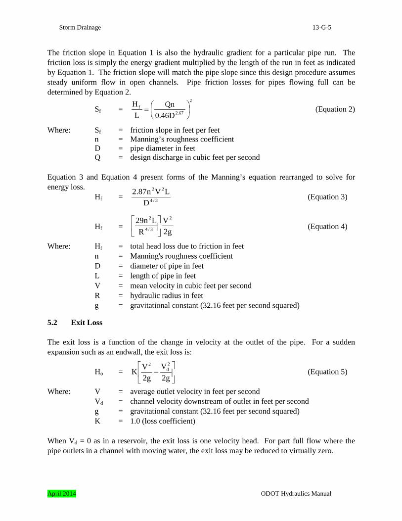
The friction slope in Equation 1 is also the hydraulic gradient for a particular pipe run. The friction loss is simply the energy gradient multiplied by the length of the run in feet as indicated by Equation 1. The friction slope will match the pipe slope since this design procedure assumes steady uniform flow in open channels. Pipe friction losses for pipes flowing full can be determined by Equation 2.

Sf = 2

67.2f

D46.0Qn

LH

= (Equation 2)

Where: Sf = friction slope in feet per feet n = Manning’s roughness coefficient D = pipe diameter in feet Q = design discharge in cubic feet per second Equation 3 and Equation 4 present forms of the Manning’s equation rearranged to solve for energy loss. Hf = (Equation 3) Hf = (Equation 4) Where: Hf = total head loss due to friction in feet n = Manning's roughness coefficient D = diameter of pipe in feet L = length of pipe in feet V = mean velocity in cubic feet per second R = hydraulic radius in feet g = gravitational constant (32.16 feet per second squared)

5.2 Exit Loss The exit loss is a function of the change in velocity at the outlet of the pipe. For a sudden expansion such as an endwall, the exit loss is: Ho = (Equation 5) Where: V = average outlet velocity in feet per second Vd = channel velocity downstream of outlet in feet per second g = gravitational constant (32.16 feet per second squared) K = 1.0 (loss coefficient) When Vd = 0 as in a reservoir, the exit loss is one velocity head. For part full flow where the pipe outlets in a channel with moving water, the exit loss may be reduced to virtually zero.

g2V

RLn29 2

3/4

2

3/4

22

DLVn87.2

−

g2V

g2VK

2d

2



5.3 Entrance Losses Entrance losses need to be considered in storm drain design only at those locations where the storm drain originates at a culvert. The energy losses associated with culvert inlets are related to the type of culvert inlet used. Entrance losses are calculated as discussed in Chapter 9.

5.4 Bend Loss The bend loss coefficient for storm drain design is minor but can be evaluated using the following formula:

Hb =

∆

g2V

0033.02o (Equation 6)

Where: Δ = angle of curvature in degrees Vo = average outlet velocity in feet per second g = gravitational constant (32.16 feet per second squared)

5.5 Access Structure Losses The head loss encountered in going from one pipe to another through an access structure is commonly represented as being proportional to the velocity head at the outlet pipe. Using K to signify this constant of proportionality, the energy loss is approximated by using the following formula. Has = (Equation 7) Experimental studies have determined that the K value can be approximated as follows: K = Ko CD Cd CQ Cp CB (Equation 8) Where: Has = head loss at access structure K = adjusted loss coefficient Ko = initial head loss coefficient based on relative access structure size CD = correction factor for pipe diameter (pressure flow only) Cd = correction factor for flow depth (non-pressure flow only) CQ = correction factor for relative flow CB = correction factor for benching Cp = correction factor for plunging flow

g2

VK2o



5.5.1 Relative Access Structure Size Ko is estimated as a function of the relative access structure size and the angle of deflection between the inflow and outflow pipes. See Figure 2. Ko = (Equation 9) Where: θ = the angle between the inflow and outflow pipes in degrees b = access structure diameter in feet Do = outlet pipe diameter in feet

Figure 2 - Deflection Angle

5.5.2 Pipe Diameter A change in head loss due to differences in pipe diameter is only significant in pressure flow situations when the depth in the access structure to outlet pipe diameter ratio, daho/Do, is greater than 3.2. Otherwise, CD is set equal to 1.0. Use the following equation when this is not the case. CD = (Equation 10) Where: CD = correction factor for pipe diameter Di = incoming pipe diameter in feet Do = outgoing pipe diameter in feet daho = water depth in access structure above the outlet pipe invert in feet

( ) θ

+θ−

sin

Db4.1sin1

Db1.0

15.0

oo

3

i

o

DD



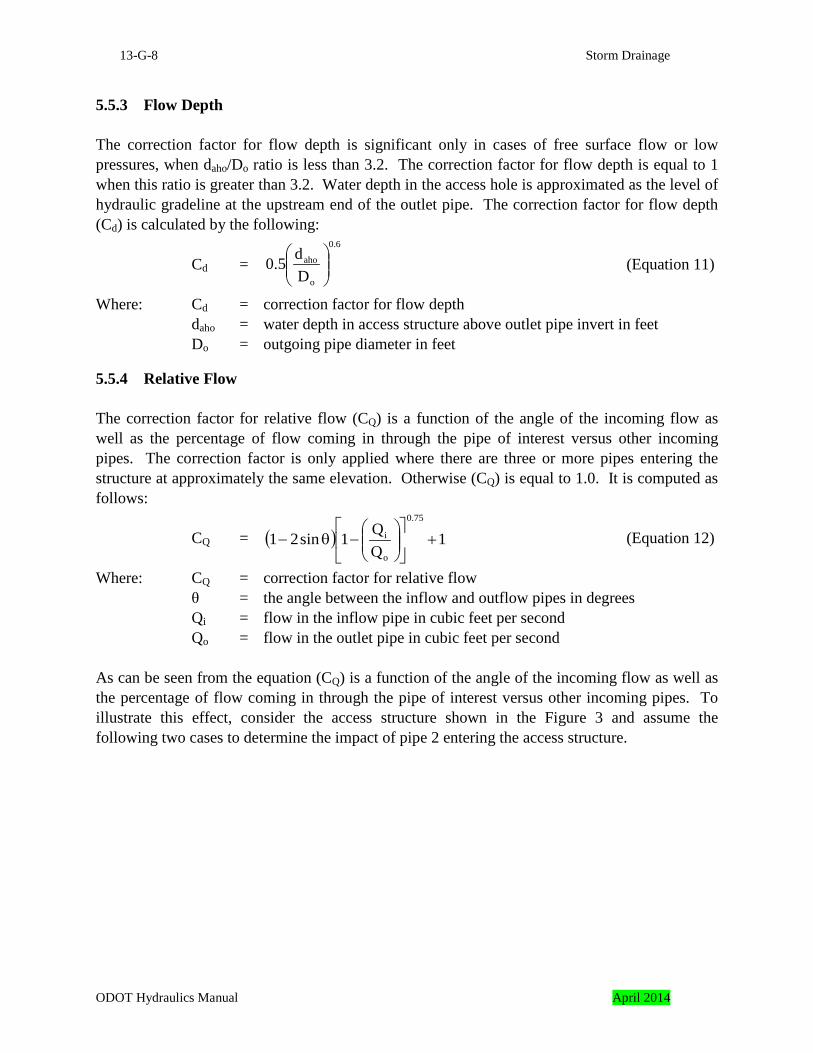
5.5.3 Flow Depth The correction factor for flow depth is significant only in cases of free surface flow or low pressures, when daho/Do ratio is less than 3.2. The correction factor for flow depth is equal to 1 when this ratio is greater than 3.2. Water depth in the access hole is approximated as the level of hydraulic gradeline at the upstream end of the outlet pipe. The correction factor for flow depth (Cd) is calculated by the following: Cd = (Equation 11) Where: Cd = correction factor for flow depth daho = water depth in access structure above outlet pipe invert in feet Do = outgoing pipe diameter in feet

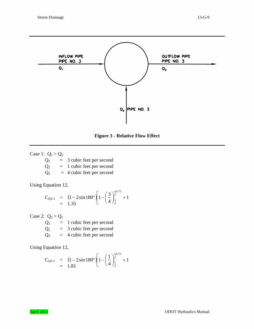
5.5.4 Relative Flow The correction factor for relative flow (CQ) is a function of the angle of the incoming flow as well as the percentage of flow coming in through the pipe of interest versus other incoming pipes. The correction factor is only applied where there are three or more pipes entering the structure at approximately the same elevation. Otherwise (CQ) is equal to 1.0. It is computed as follows: CQ = (Equation 12) Where: CQ = correction factor for relative flow θ = the angle between the inflow and outflow pipes in degrees Qi = flow in the inflow pipe in cubic feet per second Qo = flow in the outlet pipe in cubic feet per second As can be seen from the equation (CQ) is a function of the angle of the incoming flow as well as the percentage of flow coming in through the pipe of interest versus other incoming pipes. To illustrate this effect, consider the access structure shown in the Figure 3 and assume the following two cases to determine the impact of pipe 2 entering the access structure.

6.0

o

aho

Dd5.0

( ) 1QQ1sin21

75.0

o

i +

−θ−



Figure 3 - Relative Flow Effect

Case 1: Q1 > Q2

Q1 = 3 cubic feet per second Q2 = 1 cubic feet per second Q3 = 4 cubic feet per second

Using Equation 12,

CQ3-1 = = 1.35 Case 2: Q2 > Q1 Q1 = 1 cubic feet per second Q2 = 3 cubic feet per second Q3 = 4 cubic feet per second Using Equation 12,

CQ3-1 = = 1.81

( ) 1431180sin21

75.0

+

−°−

( ) 1411180sin21

75.0

+

−°−



5.5.5 Plunging Flow The correction factor for plunging flow (Cp) is calculated by the following: Cp = (Equation 13) Where: Cp = correction for plunging flow

h = vertical distance of plunging flow from flow line of incoming pipe to the center of outlet pipe in feet

Do = outgoing pipe diameter in feet daho = water depth in access structure above outlet pipe invert in feet This correction factor corresponds to the effect of another inflow pipe or surface flow from an inlet, plunging into the access hole, on the inflow pipe for which the head loss is being calculated. Using the notations in the above figure for the example, Cp is calculated for pipe 1 when pipe 2 discharges plunging flow. The correction factor is only applied when h is greater than daho. Otherwise the correction factor for plunging flow is equal to 1.

5.5.6 Benching The correction for benching in the access structure (CB) is obtained from Table B. Benching tends to direct flow through the access structure, resulting in reductions in head loss. For flow depths between the submerged and unsubmerged conditions, a linear interpolation is performed. Table C provides a table of standard ODOT benching details. Figure 4 provides a schematic of the four different types of benching.

−

+

o

aho

o Ddh

Dh2.01



Table B - Correction For Benching

Bench Type Correction Factors (CB) Submerged* Unsubmerged**

Flat Floor 1.00 1.00 Half Bench 0.95 0.15 Full Bench 0.75 0.07 Improved 0.40 0.02 * pressure flow, daho/Do > 3.2 ** free surface flow, daho/Do < 1.0

Table C ODOT Benching

Access Structure Type

Bench Type Drawing

4 foot Standard Manhole

Full Bench RD344

Standard Manhole Half Bench RD336 Shallow Manhole Half Bench RD342 Large Manhole Half Bench RD346 All inlet Boxes Flat Floor - - - - -



Figure 4 - Benching Type Schematic 6.0 Surcharged-Full Flow (Pressure Flow Conditions)

Most storm drains discharge into natural receiving streams or drainages which do not submerge the outlet of the system; however, there are locations where a storm system must discharge into a stream or river where major floods in those streams will submerge the storm drain and back water into the system. During periods of little or no flow in the storm system, backwater from these streams usually is not a problem; however, when a peak flow of design magnitude occurs in the storm system simultaneously with a high flow in the receiving stream, the system becomes “surcharged” and operates under pressure flow conditions. Under the “surcharged” condition, backwater from the receiving stream may raise the elevation of the water surface (Hydraulic Grade Line or HGL) in the system high enough that water could bubble out of manholes and inlets at low points in the highway grade.



The elevation of the HGL can be determined only after the Energy Grade Line (EGL) has been established. The EGL is a line showing the total available energy in the system (potential energy plus kinetic energy). If the sewer were of constant cross section with no manholes or angle points the EGL would have a constant and continuous slope equal to the FRICTION SLOPE, Sf . However, storm sewers are not constructed in this manner and each appurtance disrupts the flow pattern in the sewer, producing an energy loss which is indicated by a sudden drop in the elevation of the EGL. Inundation of the highway can be prevented by increasing the size of the sewer pipes downstream from those areas where the elevation of the hydraulic grade line (HGL) exceeds the elevation of the low manholes and inlets. Increasing the size of the pipe reduces the friction loss in the line. Figure 5 shows a short section of a storm sewer. In the top drawing; Pipe 2 and Pipe 3 are small, thereby inducing large friction losses as indicated by the slope of the EGL. In the bottom drawing, the size of these two pipes has been increased to reduce the friction losses, thereby lowering the elevation of the EGL and HGL to a point below the top of each manhole.

6.1 Energy Grade Line and Hydraulic Grade Line This section presents a step-by-step procedure for manual calculation of the energy grade line (EGL) and the hydraulic grade line (HGL) using the energy loss method. This has been included to aid the designer in understanding the analysis process, but the most efficient means of evaluating storm drain systems is with computer programs. The following is the procedure to design sewers for surcharged-full flow conditions. Step 1- Design the storm system with procedures outlined in Appendix F for FULL AND

PARTIAL-FULL FLOW. Assume there is free outfall from the storm sewer. Step 2- Draw a profile of the proposed sewer showing the highway grade and location of

each manhole and its cover elevation. Note elevations of low gutters. Step 3- Use tabular design sheet STORM SEWER DESIGN SHEET – SURCHARGED-

FULL FLOW (Pressure Flow Conditions), Figure 6. Step 4- Using Figure 6. Enter in Column 1 the station of the sewer outfall. Step 5- Enter in Column 2 the design discharge, Q cfs for the outfall pipe. Step 6- Enter in Column 3 the size of the outfall pipe, D in inches. Step 7- Enter in Column 4 the length of the outfall pipe, L in feet Step 8- Hydraulic structure losses and other minor pipe losses are determined and

transferred to Figure 6 in columns 9 and 13. Refer to section 5.0 for Energy Losses.



Step 9- Enter in Column 5 the average flow velocity (V) in feet per second of the outfall pipe.

Step 10- Enter in Column 6 the velocity head for the outfall pipe. Step 11- Enter in Column 7 the average flow velocity component in the outlet channel

(which is parallel to the system) - in most cases this can be considered negligible. Note: Column 7 is normally used only once to define conditions downstream from the storm drain system.

Step 12- Enter in Column 8 the velocity head for velocity in Column 7 - in most cases this

can be considered negligible.

Note: The EGL and HGL at the outfall have now been determined. The next steps apply to the storm drain system.

Step 13- Hydraulic pipe characteristics, roughness coefficients, and equations are located

in Chapter 8 to aid in manual calculations. Also, nomographs for several types of pipes are located in Chapter 8. When the appropriate nomograph is available, use the DISCHARGE (Column 2) and PIPE DIAMETER (Column 3) and note the value on the SLOPE scale. This is the FRICTION SLOPE (Sf) of the EGL. Enter this value into Column 10.

Step 14- Multiply the value in Column 10 by the LENGTH in Column 4 to determine the

FRICTION HEAD LOSS. Enter in Column 11. Step 15- Enter in Column 12 the elevation of the energy grade line (Column 16, previous

line, plus column 9) at the outlet of the drain. Step 16- Enter in Column 16 the elevation of the hydraulic grade line at the outlet of the

drain by subtracting from the value in Column 12 the value in Column 6. Step 17- Enter in Column 1 the station identification of the upstream end of the outfall

pipe. Step 18- Enter in Column 12 the elevation of the energy grade line (EGLo) at the upstream

end of the outfall pipe by adding to the first value in Column 15 (on the previous line) (FRICTION HEAD LOSS) to the value in Column 11.

Step 19- Enter in Column 14 energy losses for structures, multiply Column 13 by Column

6. Step 20- Enter in Column 15 the elevation of the energy grade line, EGLi , Column 14 is

added to Column 12 (previous line).



Step 21- Enter in Column 16 the elevation of the hydraulic grade line at the upstream end of the outlet pipe. Note: the EGL and HGL should be parallel and separated by the amount of the velocity head in the storm drain pipe (HGL = EGL – V2/2g).

Step 22- Repeat procedure starting with Step 13 for the next upstream run of pipe. Step 23- Plot the HGL and EGL on the storm sewer profile to determine if the HGL

elevation exceeds the gutter grade elevation of the highway. Step 24- If the HGL elevation is above the highway grade, the size of the pipes

downstream from the point of inundation should be enlarged to reduce the elevation of the HGL. The pipes should be enlarged sufficiently to assure the hydraulic grade line is 0.5 feet or more below the rim elevation of any drainage structure which may be affected. The EGL must also be at or below the rim elevation of any drainage structure which may be affected.

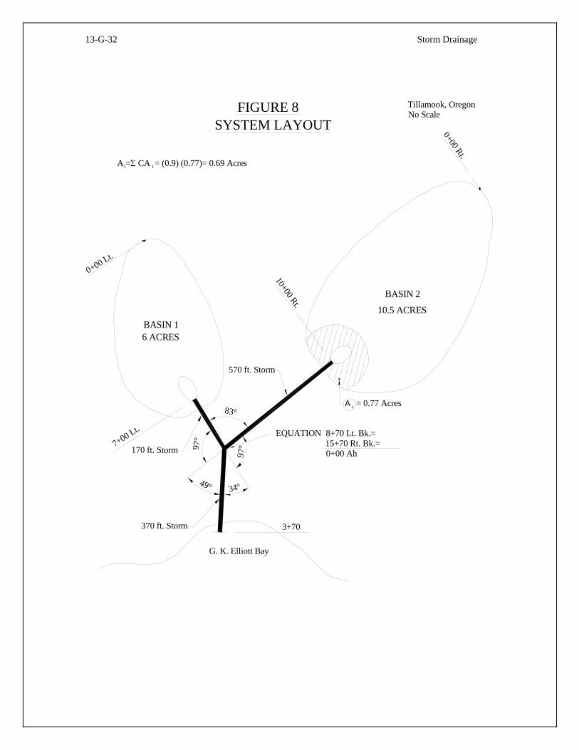
6.2 Storm Drain Design (Surcharge-full Flow) Example The following example demonstrates the design process and calculation for a double branch surcharged storm drain that is surcharged-full flow. The drain system will be designed to convey stormwater from the drainage basins displayed on Figure 7 (drainage map) to G. K. Elliot Bay which is located at Tillamook, Oregon. The double branch surcharged-full storm sewer will remove the storm water runoff from the two hatched basins shown on the Drainage Map (Figure 7). PART A. The following design steps outline the proposed storm drain system’s characteristics (i.e., preparing a drainage basin map, delineation of drainage basins, horizontal computations, collection alignments, hydrologic computations, and collection structure selection) which are necessary prior to pipe sizing design. Step A.1- Locate and sketch the storm sewer system as shown on Figure 8, 9 and 10. Add

stations from the most distant points on the basins to the outfall at G. K. Elliott Bay. An equation at the manhole was included to separate the left branch from the right branch.

Step A.2- Enter in Column 1 of “STORM SEWER DESIGN SHEET - FULL AND

PARTIAL-FULL FLOW”, Figure 11, the stations which had been sketched and located on Figure 8. A Type III non-reinforced concrete pipe will be used with a required minimum cover of 1.5 feet. A Manning’s “n” value of 0.013 will be assumed. The outfall pipe from the manhole will be sized to convey the 50-year peak design discharge.

Step A.3- Enter in Columns 2, 3, 4, 5 and 6 of Figure 11 the drainage areas Basin 1 (ΣCA =

5.4 acres) and Basin 2 (ΣCA = 9.45 acres) which are shown on Figure 7.



Step A.4- The times of concentration of 6.3 minutes (Basin 1) and 29.5 minutes (Basin 2) were used for the design of the storm sewer. These times of concentration were calculated as explained in Chapter 7. Enter these times of concentration in Columns 7 and 8 of Figure 11.

Step A.5- Obtain the 10-year rainfall intensity corresponding to durations of 6.3 minutes and

29.5 minutes in Chapter 7. Enter 2.5 inches per hour and 1.25 inches per hour in Column 9, Figure 11.

Step A.6.- Multiply Column 9 times Column 6 and enter 11.8 cubic feet per second and 13.5

cubic feet per second in Column 10 of Figure 11.

Step A.7- Two profiles which show the controlling elevation, the manhole location and the G. K. Elliott Bay receiving channel, were drawn on Figures 9 and 10. From these figures enter in Column 18 of Figure 11 the controlling ground elevations of 117.0, 110.0 and 109.5 feet. These are the elevations which must not be exceeded by the hydraulic grade line. If these elevations are exceeded, localized flooding will occur.

Step A.8- Enter in Column 15 of Figure 11 the pipe lengths of 570, 370, and 170 feet.

Step A.9- Estimate the invert slope as follows:

Right Branch Invert Slope = (117.0 – 109.5)(100) / 570 = 1.316 percent Left Branch Invert Slope = (110 – 109.5)(100) / 170 = 0.294 percent

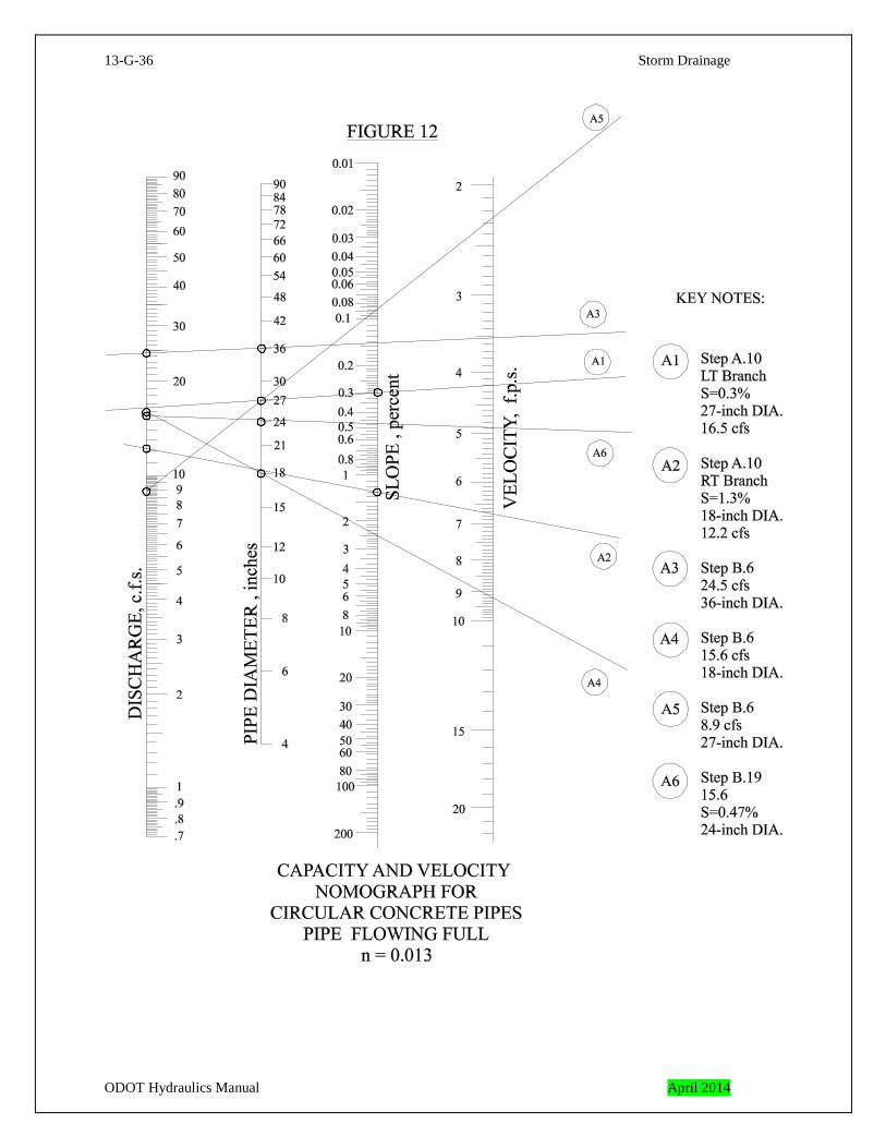
Step A.10- The previously estimated design discharges and invert slopes were used to

tabulate the pipe size, capacity flowing full and velocity flowing full for each branch. This data was determined using Figure 12 (circular concrete pipe nomograph). Enter in Columns 11, 12, 13 and 14 of Figure 11 the following table:

Note: Additional hydraulic pipe characteristics, roughness coefficients, and nomographs are located in Chapter 8.

Design Discharge, Cubic feet per Second

Invert Slope, Percent

Pipe Size,

Inches

Capacity Flowing Full,

Cubic Feet per Second

Velocity Flowing Full,

Feet per Second

RIGHT Branch 11.8 1.316 18 12.2 7.0

LEFT Branch 13.5 0.294 27 16.5 4.2



Step: A.11- Determine and enter in Column 17 of Figure 11 the minimum invert elevation for the left branch using the following relationship. Type III non-reinforced concrete pipe will be used with a required minimum cover of 1.5 feet.

Left Branch

Top of Manhole Elevation

- Pavement Thickness - Pipe

Diameter - Shell Thickness of Pipe

- Minimum Cover =

Minimum Invert Elevation

Minimum Invert Elev. Inlet End

= 110.0 - 1.0 - 1227

- 12

0.4 - 1.5 = 104.92

feet Minimum Invert Elev. Outlet End

= 109.5 - 1.0 - 1227

- 12

0.4 - 1.5 = 104.42

feet

Step A.12- Determine and enter in Column 17 of Figure 11 the minimum invert elevation for the outlet end of the Right Branch as shown below. The same relationship defined above is used to calculate this elevation. Minimum Invert Elev. Outlet End = 109.5 - 1.0 - - - 1.5 = 105.29 feet Right Branch

Step A.13- Calculate and enter in Column 17 of Figure 11 the invert elevation for the inlet

end of the Right Branch.

Invert Elev. Inlet End = 105.29 + (1.316)(570) / 100 = 112.79 feet Right Branch

Step A.14- The outfall pipe from the manhole is to be sized to convey the 50-year peak

design discharge. Both the 29.5-minute storm and the 6.3-minute storm must be investigated to determine which storm produces the peak discharge through the outfall pipe. For the longer time of concentration (29.5-minute storm), both basins will contribute runoff from 100 percent of their drainage areas. Enter in Columns 2, 3, 4, 5 and 6 of Figure 11 the total drainage area. (ΣCA = 14.85 acres)

Step A.15- For the shorter time of concentration (6.3-minute storm), 100 percent of Basin 1

and a portion of Basin 2 will contribute runoff to the outfall (Station 3+70). The following relationship was used to determine the time of contributing runoff from Basin 2 for the 6.3-minute storm. The velocity for the left and right branch was estimated to be 4.2 feet per second and 7.0 feet per second (see Figure 11), respectively.

1218

125.2



Time of Contributing

Runoff Basin 2 +

Pipe Flow Time Right

Branch =

Time of Concentration

Basin 1 +

Pipe Flow Time Left

Branch Time of

Contributing Runoff Basin 2

= ( )( ) ( )( ) minutes 61.5600.7

570602.4

1703.6 =−+

The kinematic wave equation (see Chapter 7) was used to calculate the length of contributing drainage area when I50-yr = 3.20 inches per hour for the 50-year flood, the 6.3-minute storm and a contributing time of 5.61 minutes. These calculations are shown below: Tc = 5.61 minutes I = 3.20 inches per hour n = 0.012 s = 0.001 feet per feet. Tc = (see Chapter 7) Rearranging the above equation to solve for L L = L = L = 116 feet use L = 120 feet

Step A.16- Sketch this estimated travel length of 120 feet on Figure 8 which will delineate the contributing drainage area for the 6.3-minute storm (Area A1). Enter in Columns 2, 3, 4, 5, and 6 of Figure 11 the contributing drainage area (A1 = ΣCA = 0.69 acres) from Basin 2.

Step A.17- Calculate and enter in Column 7 the flow time through the right and left branches

using the following relationship.

Right branch: Tc = L / V = 570 /(7.0)(60) = 1.4 minutes Left branch: Tc = L / V = 170 /(4.2)(60) = 0.7 minutes

3.04.0

6.06.0

SInL93.0

67.1

6.0

3.04.0c

n93.0SIT

( )( ) ( )( )

67.1

6.0

3.04.0

012.093.0001.020.361.5



Step A.18- Add the flow times calculated above to the previous total time of concentration and enter the following results in Column 8. 29.5 minutes + 1.4 minutes = 30.9 minutes (total time of concentration for right branch) 6.3 minutes + 0.7 minutes = 7.0 minutes (total time of concentration for left branch)

Step A.19- Obtain the 50-year rainfall intensity corresponding to durations of 30.9 and 7.0 minutes using the Zone 2 Intensity-Duration-Frequency curve (Chapter 7). Enter 1.65 inches per hour and 3.20 inches per hour in Column 9, Figure 11.

Step A.20- Multiply Column 9 times Column 6 and enter 24.5 cubic feet per second and 19.5

cubic feet per second in Column 10 of Figure 11. The outfall pipe will be sized to convey 24.5 cubic feet per second, the greater peak discharge.

Step A.21- For Station 3+ 70, enter in Column 17 the Invert Elevation of 99.6 feet. The

elevation places the outlet of the outfall pipe at the bottom of the channel. An outlet velocity of approximately 3.0 feet per second would minimize erosion at the end of the outfall pipe.

Step A.22- Given a design discharge of 24.5 cubic feet per second, determine slope, pipe

size, and velocity for the outfall, Station 3+ 70. Using Figure 12, enter in Columns 11, 12, 13 and 14 of Figure 11 for the outfall pipe 0.145 percent, 36-inch, 24.5 cubic feet per second and 3.6 feet per second. The 36-inch diameter pipe is the smallest standard size pipe which can carry the design flow (24.5 cubic feet per second) and also satisfy the minimum velocity criterion (3 feet per second).

Step A.23- For the outfall pipe, Station 0+ 00 Ah to Station 3+ 70, determine fall and enter in

Column 16 as shown below:

Fall = (0.145) (370) / 100 = 0.67 feet

Step A.24- Calculate and enter in Column 17 the Invert Elevation as shown below:

99.6 + 0.67 = 100.27 feet This will be the invert elevation at Station 0+ 00 Ah.

PART B. Check the storm sewer design as a surcharged full flow (pressure flow) system by determining the energy and hydraulic grade lines. The 50-year storm is the design storm for the surcharged condition.



Step B.1- Enter in Column 1 of “STORM SEWER DESIGN SHEET - SURCHARGED FLOW”, Figure 13, the stations shown on Figure 8 beginning with the sewer outfall at 3+ 70. Note two entries are required, one for the left branch and one for the right branch.

Step B.2- Enter in Columns 2, 3, and 4 for both branches of Figure 13 the Discharge (24.5

cubic feet per second), the Pipe Size (36-, 18- and 27-inch) and Pipe Lengths (370, 570 and 170 feet) from Figure 11.

Step B.3- Enter in Columns 5 and 6 the velocity of 3.6 feet per second and the velocity head

of 0.20 feet. The velocity head is calculated as shown below.

Velocity Head = 2gV2

= 4.64

6.3 = 0.20 feet

Step B.4- Since the average velocity component in G. K. Elliott Bay is negligible, enter in

Columns 7 and 8 the velocity of 0 feet per second and the velocity head of 0 feet.

Step B.5- Calculate and enter in Columns 2, 5 and 6, the discharge, velocity and velocity head for the right and left branches as shown below.

Q = QLt + QRt = 24.5 cubic feet per second

QRt = CIA = (9.45)(1.65)

= 15.59 cubic feet per second

QRt = CIA = 15.6 cubic feet per second

QLt = (5.40)(1.65)

= 8.91 cubic feet per second

QLt = 8.9 cubic feet per second

QRt + QLt = 24.5 cubic feet per second

A18" = 1.77 square feet VRt = = = 8.8 feet per second

A27" = 3.97 square feet VLt = = = 2.2 feet per second

= 1.21 feet = 0.08 feet

Step B.6- Enter Figure 12 using the discharges of 24.5 cubic feet per second, 15.6 cubic feet per second and 8.9 cubic feet per second (Column 1) and the pipe sizes of 36 inches, 18 inches and 27 inches (Column 2), to obtain 0.145, 2.30 and 0.090 percent from the slope scale. These are the Friction Slopes, Sf, of the EGL. Enter these friction slopes in Column 10.

AQ

77.16.15

AQ

97.36.15

g2V2

RTg2

V2LT



Step B.7- Multiply the Friction Slopes in Column 10 times the Pipe Length in Column 4 and enter in Column 11 the following results. Outfall Friction Head Loss = = 0.54 feet Right Branch Friction Head Loss = = 13.11 feet Left Branch Friction Head Loss = = 0.15 feet

Step B.8- Calculate and enter in Column 14 (Figure 13) the minor energy loss in the manhole (reference section 5.5).

Calculate the adjusted loss coefficient (K) and enter into Column 13 (Figure 13)

Has =

2gV

K2o

K = Ko CD Cd CQ CP CB (Equation 8)

Where: Has = energy loss across access hole in feet Vo = outlet velocity in feet per second g = acceleration due to gravity (32.2 feet per second

squared) K = adjusted loss coefficient Ko = initial headloss coefficient based on relative access hole

size CD = correction factor for pipe diameter (pressure flow only) Cd = correction factor for flow depth CQ = correction factor for relative flow CP = correction factor for plunging flow CB = correction factor for benching

Calculate (Ko):

Ko = ( ) θ

+θ−

ins

Db1.4 ins1

Db0.1

0.15

oo

(Equation 9)

θ = the angle between inflow and outflow pipes in degrees b = access structure diameter in feet Do = outlet pipe diameter in feet

100)370)(145.0(

100)570)(30.2(

100)170)(090.0(



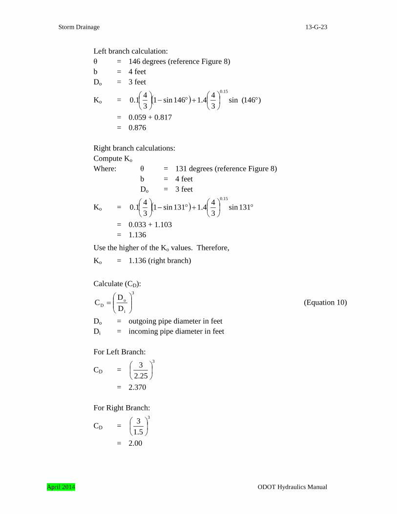
Left branch calculation: θ = 146 degrees (reference Figure 8) b = 4 feet Do = 3 feet

Ko = ( ) )461( ins341.4461 ins1

340.1

0.15

°

+°−

= 0.059 + 0.817 = 0.876 Right branch calculations: Compute Ko Where: θ = 131 degrees (reference Figure 8) b = 4 feet Do = 3 feet

Ko = ( ) °

+°−

131 ins

341.4131 ins1

340.1

0.15

= 0.033 + 1.103 = 1.136

Use the higher of the Ko values. Therefore,

Ko = 1.136 (right branch)

Calculate (CD):

3

i

oD D

DC

= (Equation 10)

Do = outgoing pipe diameter in feet Di = incoming pipe diameter in feet For Left Branch:

CD = 3

2.253

= 2.370 For Right Branch:

CD = 3

1.53

= 2.00



Is the ratio of daho/Do greater than 3.2? If not, CD = 1.0 daho = water depth in access hole above the outlet pipe invert, feet daho = HGL = invert elevation Invert EL = 100.27 feet (Figure 11, Column 17) HGL EL = 107.54 feet (Figure 13, Column 16) daho = 107.54 – 100.27 = 7.27

o

aho

Dd

= 327.7 = 2.4 which is less than 3.2, therefore CD = 1.0

Calculate (Cd):

Cd = 0.6

o

aho

Dd

0.5

(Equation 11)

= 0.6

37.270.5

= 0.85

However, if the ratio of daho/Do is greater than 3.2, then Cd = 1.0

o

aho

Dd =

37.27 = 2.4 which is less than 3.2

Therefore, Cd = 0.85

Calculate (CQ):

This correction factor is only applied to situations where there are three or more incoming pipes at approximately the same elevation. Otherwise, CQ is equal to 1.0. This example problem has two incoming pipes. Therefore, CQ = 1.0.

Calculate (Cp):

Cp =

−

+

o

aho

o Ddh

Dh0.21 (Equation 13)

Where: h = vertical distance of plunging flow from the flow line of the higher elevation inlet pipe to the center of the outflow pipe.

The two inflow pipes are at the same invert elevation and this is not a manhole with an inlet grate. Therefore,

Cp = 1.0



Calculate (CB):

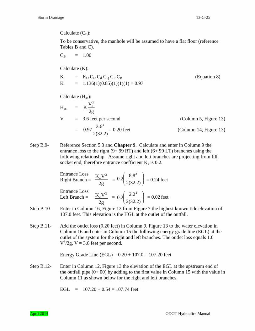
To be conservative, the manhole will be assumed to have a flat floor (reference Tables B and C).

CB = 1.00 Calculate (K):

K = KO CD Cd CQ CP CB (Equation 8) K = 1.136(1)(0.85)(1)(1)(1) = 0.97 Calculate (Has):

Has = 2gV

K2o

V = 3.6 feet per second (Column 5, Figure 13)

= 2(32.2)

6.397.02

= 0.20 feet (Column 14, Figure 13)

Step B.9- Reference Section 5.3 and Chapter 9. Calculate and enter in Column 9 the entrance loss to the right (9+ 99 RT) and left (6+ 99 LT) branches using the following relationship. Assume right and left branches are projecting from fill, socket end, therefore entrance coefficient Ke is 0.2. Entrance Loss Right Branch = = = 0.24 feet Entrance Loss Left Branch = = = 0.02 feet

Step B.10- Enter in Column 16, Figure 13 from Figure 7 the highest known tide elevation of 107.0 feet. This elevation is the HGL at the outlet of the outfall.

Step B.11- Add the outlet loss (0.20 feet) in Column 9, Figure 13 to the water elevation in

Column 16 and enter in Column 15 the following energy grade line (EGL) at the outlet of the system for the right and left branches. The outlet loss equals 1.0 V2/2g, V = 3.6 feet per second.

Energy Grade Line (EGL) = 0.20 + 107.0 = 107.20 feet

Step B.12- Enter in Column 12, Figure 13 the elevation of the EGL at the upstream end of

the outfall pipe (0+ 00) by adding to the first value in Column 15 with the value in Column 11 as shown below for the right and left branches.

EGL = 107.20 + 0.54 = 107.74 feet

g2VK 2

e

)2.32(2

8.82.02

g2VK 2

e

)2.32(2

2.22.02



Step B.13- Subtract 0.20 (Column 6) from 107.74 (Column 12) and enter in Column 16 the HGL elevation 107.54 feet for the right and left branches.

Step B.14- Enter in Column 18 the top of manhole elevation 109.5 feet (see Figure 7).

Step B.15- The elevation of the EGL inside the manhole is calculated by adding the manhole

loss to the EGL of the outfall pipe.

EGL = 0.20 + 107.74 = 107.94 feet

Step B.16- The EGL and HGL calculations for the right (18-inch pipe) and left branch (27-inch pipe) upstream runs of pipe are shown in the following table.

FOR 18-INCH PIPE ON RIGHT SIDE

STA. VELOCITY HEAD

HEAD LOSS, Feet

EGL ELEV RIGHT, Feet

HGL ELEV RIGHT, Feet

0+00 Rt M.H. 15+70 Rt 10+00 Rt 9+99 Rt

0.20 1.21 1.21 0.00

0.20 13.11 0.24

107.74 107.94 107.94 121.05 121.29

107.54 106.73 119.84 121.29

FOR 27-INCH PIPE ON LEFT SIDE 0+00 Lt M.H. 8+70 Lt 7+00 Lt 6+99 Lt

0.20 0.08 0.08 0.00

0.20 0.15 0.02

107.74 107.94 107.96 108.11 108.13

107.54 107.88 108.03 108.13

Step B.17- Second design attempt with 24-inch pipe for the Right Branch. Need to determine

the EGL and HGL. As shown in the table above, the proposed upstream run of 18-inch pipe for the right branch would result in an improper design as shown on Figure 1. The calculated EGL and HGL elevation of 121.29 feet exceeds the natural ground elevation of 117.0 feet shown on Figure 10. For a proper design the EGL and HGL elevation must be below elevation 117.0 feet. A 24-inch will be investigated with its design information tabulated below. The information below will be used in Figure 13.

Design

Discharge Invert Slope

Pipe Size

Capacity Flowing Full

Velocity Flowing Full

RIGHT Branch 11.8 cfs 0.27 % 24-inch 11.8 cfs 3.7 fps

Step B.18- Calculate as shown below the velocity and velocity head for a 24-inch pipe which

would convey a discharge of 15.6 cfs (see step 5 above). Enter the values in Columns 5 and 6.



A24 in. = 3.142 square feet VRt = = = 5.0 feet per second = 0.39 feet

Step B.19- Enter Figure 12 using the discharge of 15.6 cubic feet per second (Column 1) and

the 24-inch pipe (Column 2) to obtain 0.47 percent from the slope scale. Enter in Column 10 the friction slope of 0.47 percent.

Step B.20- Multiply the friction slope in Column 10 times the pipe length in Column 4 and

enter in Column 11 the following result.

Friction = = 2.68 feet Head Loss

Step B.21- Estimate the minor energy loss in the manhole with the 24-inch pipe using the

following relationships presented in Section 5.5. The minor energy loss will remain the same as computed in Step 8. Has = 0.20 feet

Step B.22- The elevation of the EGL inside the manhole is calculated by adding the manhole

loss to the EGL of the outfall pipe.

EGL = 0.20 + 107.74 = 107.94 feet

Step B.23- The EGL and HGL calculations for the right and left branch upstream runs of pipe are shown in Figure 13.

Step B.24- As shown in Figure 13 both the right and left branches are proper designs. The

HGL and EGL are below the control points.

Step B.25- Change the entries in Columns 11,12,13 and 14 for the Right Branch from 1.316 percent, 18-inch, 12.2 cubic feet per second and 7.0 feet per second to 0.27 percent, 24-inch, 11.8 cubic feet per second and 3.7 feet per second as shown in Figure 11.

Step B.26- Determine and enter in Column 17 of Figure 11 the minimum invert elevation for

the outlet end of the 24-inch pipe as shown below. The relationship from Step 11, Part A, was used to calculate the invert elevation.

Minimum Invert Elev. = 109.5 - 1.0 - - - 1.5 = 104.75 feet Outlet End Right Branch

Step B.27- Estimate and enter in Column 17 of Figure 11 the invert elevation for the inlet end of the 24-inch pipe using the following relationship.

AQ

142.36.15

g2V2

RT

100)570)(47.0(

1224

120.3



Invert Elev. = 104.75 + = 106.29 feet Inlet End Right Branch

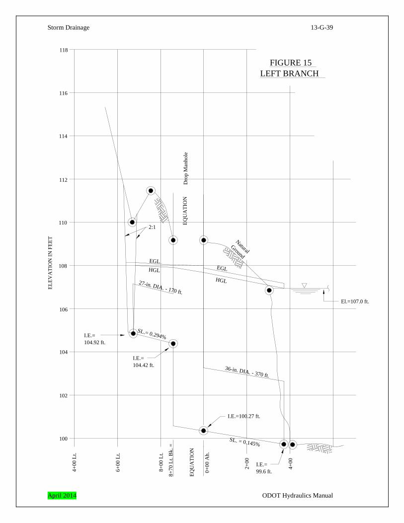
Step B.28- Sketch the storm system, the HGL and EGL on Figures 14 (Right Branch) and 15

(Left Branch).

100)570(27.0



SYSTEM LAYOUTFIGURE 8

BASIN 1

BASIN 2

A =Σ CA = (0.9) (0.77)= 0.69 Acres

0+00 Lt.

7+00 Lt.

= 0.77 Acres

Tillamook, OregonNo Scale

G. K. Elliott Bay

EQUATION

10+00 Rt.

A 1

0+00 Rt.

3+70

8+70 Lt. Bk.=15+70 Rt. Bk.=0+00 Ah

1

6 ACRES

10.5 ACRES

570 ft. Storm

170 ft. Storm

370 ft. Storm

49° 34°

97°

97°

83°

1


Σ

Drainge Area Runoff

1a 2 3 4 5 6 7 8 9 10 11 12 13 14 15 16 17 18 19

Station

10+00 Rt

7+00 Lt

3+70

0+00 Lt

7+00 Lt

3+70

Index No. Area Coeff.

A C

Remarks

10.52 .9 9.4529.5 29.5

11.80.27 570

100.27 109.5

117.0

99.6

(outfall)

FIGURE 11STORM DRAIN DESIGN SHEET

FULL AND PARTIAL-FULL FLOW

c c

PROJECT: Example Problem DESIGN FREQUENCY: 10- Year DESIGNED BY: JOE SMITH DATE: 2005 * 50- Year

Acres

15+70 Rt Bk 0+00 Ah

1 6.0 .9 5.40

9.45

14.851.4 30.9

1.25

*1.6524.5

1.316

0.145

2418

11.812.2

3.77.0

1.547.50

104.75105.29

106.29112.79

(in)(out)

36 24.5 3.6 3700.67

99.6

1

A1

8+70 Lt Bk 0+00 Ah

6.0 .9 5.406.3 6.3

13.5

5.402.50

0.294 27 16.5 4.2 1700.50

104.92

104.42100.27

110.0

109.5(in)

(out)

0.77 .9 0.690.7 7.0

19.5

6.09*3.20

0.145 36 24.5 3.6 3700.67

(outfall)

Equiv. Areafor 100%Runoff

CA(3) x (4)

TotalImpervious

DrainageArea

CAAcres

Time ofConcent.or FlowTime, T

Minutes

TotalTime ofConcent.

T

Minutes

AverageRainfallIntensity I

in/hr

DesignDischarge

Q (6) x (9)

cfs

InvertSlope S

%

PipeSize D

Inches

CapacityFlowing Full Q

cfs

VelocityFlowing Full V

fps

Length

L

feet

Fall

feet

InvertElevation

feet

Top ofManholeElevation

feet

f f

1b

Node I.D.



1a 2 3 4 5 6 7 8 9 10 11 12 13 14 15 19

Station Discharge Remarks

PROJECT: Example Problem DESIGN FREQUENCY: 50-Year DESIGNED BY: JOE SMITH DATE: 2005

1 2

PIPE DATA HEAD LOSSES

f

K

0

16 17

i

18I.D. cfs

3+70

15+70 Rt

10+00 Rt

9+99 Rt

36 0.20 0.20

570

3.6

0.145

0.47 2.68

0.020.090

0.54

0+00 Ah

10+00 Rt

9+99 Rt

24.5

15.6

0.0 0.0

0.54

107.00

107.74

107.94

107.00

107.54109.50

110.62

107.74

110.23

110.70

107.00

108.29

3+70 Lt0+00 Ah

OutfallJust inside pipe at outfall pipe

Just inside inlet end of outfall pipeInside manhole

2nd Try

Does not exceed ground elevationsDesign is okay

Inside manhole

15.6

24.5 36

18

18

370 0.203.6 0.00.97 0.20

107.20

107.94

102.60

103.27

570

8.8

8.8

1.21

1.21 2.30 13.11 121.05

Just inside pipe as it enters manhole

Just inside outlet of pipe

Exceeds ground level, try next size pipe

15+70 Rt 570

15.6

15.6

24

24

570

5.0

5.0

.39

.39

8+70 Lt7+00 Lt6+99 Lt

24.5 36 3.6 .20

8.9 27 2.2 .088.9 27 2.2 .08

170170

0.02

0.24

0.08

107.94

106.73

119.84

121.29 121.29

0.145

0.15 108.11107.96

0.97 0.20

110.70

107.20

107.94

108.13

107.88

108.13

106.67

107.17

109.50

110.00

Just inside pipe as it enters manholeJust inside outlet pipeJust outside inlet end of pipeHGL & EGL do not exceed groundelevations. Design is OK

106.75

117.00

12

22

feet

___2g

___2g

107.55

107.54 103.27Just inside pipe at outfallJust inside inlet end of outfall pipe

Outfall

107.00 107.00Outfall107.0

Outfall

V 2__2g

Minor Pipe

Losses

PipeSize

Dinches

PipeLength

L feet

V

feet

V

fps

V

feet

V

fps

Friction Slope

S %

Friction Head Loss

(4) x (10)

feet

EnergyGradeLine

EGL feet

K

feet

EGL

feet

Piezometricor waterSurface

(HGL) feet

Crown ofPipe

feet

Low Gutter/Surface

Elevation

feet

FIGURE 13STORM DRAIN DESIGN SHEET

SURCHARGED FLOW (Pressure Flow Conditions)

0.0 0.0

108.03

117.00

1b

Node I.D.

102.6



8+00

Rt.

106

108

110

104

10+0

0R

t.

118

112

114

116

12+0

0R

t.

14+0

0R

t.

15+7

0R

t.B

k.=

Equa

tion

2+00

4+000+

00A

h

36-in. DIA. - 370 ft.

24-in. DIA. - 570 ft.

EGL

HGL

SL. = 0.27%

EGLHGL

NA

TURA

LG

ROU

ND

NATURAL GROUND

2:1

FIGURE 14RIGHT BRANCH

Dro

pM

anho

le

102

100 SL. = 0.145%

ELEV

ATI

ON

INFE

ET

I.E.=106.29 ft.

I.E.=104.75 ft.

I.E.=100.27 ft. I.E.=

99.60 ft.

El.=107.00 ft.



FIGURE 15LEFT BRANCH

4+00

Lt.

106

108

110

104

6+00

Lt.

118

112

114

116

8+00

Lt.

0+00

Ah.

2+00

4+00

2:1

102

100 SL. = 0.145%

8+70

Lt.

Bk.

=

EQU

ATI

ON

36-in. DIA. - 370 ft.

SL.= 0.294%

EQU

ATI

ON

Dro

p M

anho

le

27-in. DIA. - 170 ft.

EGL

HGL

EGLHGL

NaturalGround

ELEV

ATI

ON

IN F

EET

El.=107.0 ft.

I.E.=100.27 ft.

I.E.=99.6 ft.

I.E.=104.42 ft.

I.E.=104.92 ft.


APPENDIX G HYDRAULIC GRADE LINE 1.0 … · April 2014 ODOT Hydraulics Manual . 13-G-2 Storm...

Documents

Transcript of APPENDIX G HYDRAULIC GRADE LINE 1.0 … · April 2014 ODOT Hydraulics Manual . 13-G-2 Storm...