APPENDIX F - Finger Lakes LPG Storage · establishing a suitable factor of safety against slope ......
102
APPENDIX F Geotechnical References
Transcript of APPENDIX F - Finger Lakes LPG Storage · establishing a suitable factor of safety against slope ......

APPENDIX F
Geotechnical References

Analysis and design of veneer cover soils
R. M. Koerner1 and T.-Y. Soong2
1Emeritus Proffesor, Drexel University and Director, Geosynthetic Research Institute, 475 Kedron
Avenue, Folsom, PA 19033-1208, USA, Telephone: +1 610 522 8440, Telefax: +1 610 522 8441,
E-mail: [email protected] and Associates, 12842 Emerson Drive, Brighton, MI 48116, USA, Telephone: +1 248 846 5100,
Telefax: +1 248 846 5101, E-mail: [email protected]
Received 10 July 2003, accepted 10 July 2003
ABSTRACT: Cover soil sliding on slopes underlain by geosynthetics is obviously an unacceptable
situation and, if the number of occurrences becomes excessive, can eventually reflect poorly on the
entire technology. Steeply sloped leachate collection layers and final covers of landfills are
situations where incidents of such sliding have occurred. Paradoxically, the analytic formulation of
the situation is quite straightforward. This paper presents an analysis of the common problem of a
veneer of cover soil (0.3 to 1.0 m thick) on a geosynthetic material at a given slope angle and
length. The paper then presents different scenarios that create lower FS (factor of safety) -values
than the gravitational stresses of the above situation, e.g. equipment loads, seepage forces and
seismic loads. As a counterpoint, different scenarios that create higher FS-values also are presented,
e.g. toe berms, tapered thicknesses and veneer reinforcement. In this latter category, a subdivision
is made into intentional reinforcement (using geogrids or high-strength geotextiles) and non-
intentional reinforcement (cases where geosynthetics overlay a weak interface within a multilined
slope). A standard numeric example is used in each of the above situations to illustrate the various
influences on the resulting FS-value. In many cases, design curves are also formulated. Suggested
minimum FS-values are presented for final closures of landfills, waste piles, leach pads, etc.,
which are the situations where veneer slides of this type are the most serious. Hopefully, the paper
will serve as a vehicle to bring a greater awareness to this situation so as to avert such slides
from occurring in the future. Note: This paper was initially published as the Giroud Lecture in the
Proceedings of the Sixth International Geosynthetics Conference held in Atlanta, USA, in 1998.
KEYWORDS: Geosynthetics, Analysis, Design, Limit equilibrium methods, Steep slopes, Veneer
stability
REFERENCE: Koerner, R. M. & Soong, T-Y. (2005). Analysis and design of veneer cover soils.
Geosynthetics International, Special Issue on the Giroud Lectures, 12, No. 1, 28–49
1. INTRODUCTION
There have been numerous cover soil stability problems in
the past, resulting in slides that range from being relatively
small (which can be easily repaired), to very large
(involving litigation and financial judgments against the
parties involved). Furthermore, the number of occurrences
appears to have increased over the past few years. Soong
and Koerner (1996) report on eight cover soil failures
resulting from seepage-induced stresses alone. While such
slides can occur in transportation and geotechnical appli-
cations, it is in the environmental applications area where
they are most frequent. Specifically, the sliding of rela-
tively thin cover soil layers (called ‘veneer’) above both
geosynthetic and natural soil liners, i.e. geomembranes
(GM), geosynthetic clay liners (GCL) and compacted clay
liners (CCL), are the particular materials of concern.
These situations represent a major challenge due (in part)
to the following reasons:
• The underlying barrier materials generally represent a
low interface shear strength boundary with respect to
the soil placed above them.
• The liner system is oriented precisely in the direction
of potential sliding.
• The potential shear planes are usually linear and are
essentially uninterrupted along the slope.
• Liquid (water or leachate) cannot continue to percolate
downward through the cross-section owing to the
presence of the barrier material.
When such slopes are relatively steep and uninterrupted in
Geosynthetics International, 2005, 12, No. 1
281072-6349 # 2005 Thomas Telford Ltd

their length (which is the design goal for landfills, waste
piles and surface impoundments so as to maximize
containment space and minimize land area), the situation
is exacerbated.
There are two specific applications in which cover soil
stability has been difficult to achieve in light of this
discussion;
• leachate collection soil placed above a GM, GCL and/
or CCL along the sides of a landfill before waste is
placed and stability achieved accordingly;
• final cover soil placed above a GM, GCL and/or CCL
in the cap or closure of a landfill or waste pile after the
waste has been placed to its permitted height.
For the leachate collection soil situation the time frame is
generally short (from months to a few years), and the
implications of a slide may be minor in that repairs can
sometimes be done by on-site personnel. For the final
cover soil situation the time frame is invariably long (from
decades to centuries), and the implications of a slide can
be serious in that repairs often call for a forensic analysis,
engineering redesign, separately engaged contractors and
quite high remediation costs. These latter cases sometime
involve litigation, insurance carriers, and invariably tech-
nical experts, thus becoming quite contentious.
Since both situations (leachate collection and final
covers) present the same technical issues, the paper will
address them simultaneously. It should be realized, how-
ever, that the final cover situation is of significantly
greater concern.
In the sections to follow, geotechnical engineering
considerations will be presented leading to the goal of
establishing a suitable factor of safety against slope
instability. A number of common situations will then be
analyzed, all of which have the tendency to decrease
stability. A number of design options will follow, all of
which have the objective of increasing stability. A sum-
mary and conclusions section will counterpoint the various
situations which tend to either create slope instability or
aid in slope stability. It is hoped that an increased
awareness of the analysis and design details offered here-
in, and elsewhere, will lead to a significant decrease in the
number of veneer cover soil slides that have occurred.
2. GEOTECHNICAL ENGINEERINGCONSIDERATIONS
As just mentioned, the potential failure surface for veneer
cover soils is usually linear with cover soil sliding with
respect to the lowest interface friction layer in the under-
lying cross-section. The potential failure plane being linear
allows for a straightforward stability calculation without
the need for trial center locations and different radii, as
with soil stability problems analyzed by rotational failure
surfaces. Furthermore, full static equilibrium can be
achieved without solving simultaneous equations or mak-
ing simplified design assumptions.
2.1. Limit equilibrium concepts
The free body diagram of an infinitely long slope with
uniformly thick cohesionless cover soil on an incipient
planar shear surface, like the upper surface of a geomem-
brane, is shown in Figure 1. The situation can be treated
quite simply. By taking force summation parallel to the
slope and comparing the resisting force with the driving or
mobilizing force, a global factor of safety (FS) results:
FS ¼
X
Resisting forces
X
Driving forces
¼ N tan ä
W sin â¼ W cos â tan ä
W sin â
(1a)
Hence:
FS ¼ tan ä
tan â(1b)
Here it is seen that the FS-value is the ratio of tangents of
the interface friction angle of the cover soil against the
upper surface of the geomembrane (ä), and the slope
angle of the soil beneath the geomembrane (â). As simple
as this analysis is, its teachings are very significant. For
example:
• To obtain an accurate FS-value, an accurately
determined laboratory ä-value is absolutely critical.
The accuracy of the final analysis is only as good as
the accuracy of the laboratory-obtained ä-value.
• For low ä-values, the resulting soil slope angle will be
proportionately low. For example, for a ä-value of 208,
and a required FS-value of 1.5, the maximum slope
angle is 148. This is equivalent to a 4(H) on 1(V) slope,
which is relatively low. Furthermore, many geomem-
branes have even lower ä-values than 208.
• This simple formula has driven geosynthetic manufac-
turers to develop products with high ä-values, e.g.
textured geomembranes, thermally bonded drainage
geocomposites, internally reinforced GCLs, etc.
Unfortunately, the above analysis is too simplistic to use
in most realistic situations. For example, the following
situations cannot be accommodated:
WcosâW
Wsinâ
N tanä
Cover s
oil
â N
Geomembrane
Figure 1. Limit equilibrium forces involved in an infinite
slope analysis for a uniformly thick cohesionless cover soil
Analysis and design of veneer cover soils 29
Geosynthetics International, 2005, 12, No. 1

• a finite-length slope with the incorporation of a passive
soil wedge at the toe of the slope;
• the incorporation of equipment loads on the slope;
• consideration of seepage forces within the cover soil;
• consideration of seismic forces acting on the cover soil;
• the use of soil masses acting as toe berms;
• the use of tapered covered soil thicknesses;
• reinforcement of the cover soil using geogrids or high-
strength geotextiles.
These specific situations will be treated in subsequent
sections. For each situation, the essence of the theory will
be presented, followed by the necessary design equations.
This will be followed, in each case, with a design graph
and a numeric example. First, however, the important issue
of interface shear testing will be discussed.
2.2. Interface shear testing
The interface shear strength of a cover soil with respect to
the underlying material (often a geomembrane) is critical
to properly analyze the stability of the cover soil. This
value of interface shear strength is obtained by laboratory
testing of the project-specific materials at the site-specific
conditions. By project-specific materials, we mean sam-
pling of the candidate geosynthetics to be used at the site,
as well as the cover soil at its targeted density and
moisture conditions. By site-specific conditions we mean
normal stresses, strain rates, peak or residual shear
strengths and temperature extremes (high and/or low).
Note that it is completely inappropriate to use values of
interface shear strengths from the literature for final cover
soil design.
While the above list of items is formidable, at least the
type of test is established. It is the direct shear test which
has been utilized in geotechnical engineering testing for
many years. The test has been adapted to evaluate
geosynthetics and is designated as ASTM D5321 or ISO
12957.
In conducting a direct shear test on a specific interface,
one typically performs three replicate tests, with the only
variable being different values of normal stress. The
middle value is usually targeted to the site-specific condi-
tion, with a lower and higher value of normal stress
covering the range of possible values. These three tests
result in a set of shear displacement against shear stress
curves: see Figure 2a. From each curve, a peak shear
strength (ôp) and a residual shear strength (ôr) is obtained.
As a next step, these shear strength values, together with
their respective normal stress values, are plotted in Mohr–
Coulomb stress space to obtain the shear strength para-
meters of friction and adhesion: see Figure 2b.
The points are then connected (usually with a straight
line), and the two fundamental shear strength parameters
are obtained. These shear strength parameters are: ä, the
angle of shearing resistance, peak and/or residual, of the
two opposing surfaces (often called the interface friction
angle); and ca, the adhesion of the two opposing surfaces,
peak and/or residual (synonymous with cohesion when
testing fine-grained soils).
Each set of parameters constitutes the equation of a
straight line, which is the Mohr–Coulomb failure criterion
common to geotechnical engineering. The concept is read-
ily adaptable to geosynthetic materials in the following
form:
ôp ¼ cap þ ón tan äp (2a)
ôr ¼ car þ ón tan är (2b)
The upper limit of ä when soil is involved as one of the
interfaces is ö, the angle of shearing resistance of the soil
component. The upper limit of the ca value is c, the
cohesion of the soil component. In the slope stability
analyses to follow, the ca term will be included for the
sake of completeness, but then it will be neglected (as
being a conservative assumption) in the design graphs and
numeric examples. To utilize an adhesion value, there
must be a clear physical justification for the use of such
values when geosynthetics are involved. Only unique
situations such as textured geomembranes with physical
interlocking of soils having cohesion, or the bentonite
component of a GCL, are valid reasons for including such
a term.
Note that residual strengths are equal to, or lower, than
peak strengths. The amount of difference is very depen-
dent on the material, and no general guidelines can be
given. Clearly, material-specific and site-specific direct
shear tests must be performed to determine the appropriate
values. Further, each direct shear test must be conducted
to a relatively large displacement to determine the residual
behavior (Stark and Poeppel 1994). The decision as to the
use of peak or residual strengths in the subsequent analy-
Shear displacement
(a)
Shear
str
ess
Shear
str
ength
, ô
Normal stress, ón
(b)
(Peak)
(Residual)
ón (high)
ón (middle)
ón (low)
ôr
ôp
äp
är
cap car
Figure 2. Direct shear test results and method of analysis to
obtain shear strength parameters: (a) direct shear test data;
(b) Mohr–Coulomb stress space
30 Koerner and Soong
Geosynthetics International, 2005, 12, No. 1

sis is a very subjective one. It is both a materials-specific
and site-specific issue, which is left up to the designer
and/or regulator. Even further, the use of peak values at
the crest of a slope and residual values at the toe may be
justified. As such, the analyses to follow will use an
interface ä-value with no subscript, thereby concentrating
on the computational procedures rather than this particular
detail. However, the importance of an appropriate and
accurate ä-value should not be minimized.
Owing to the physical structure of many geosynthetics,
the size of the recommended shear box is quite large. It
must be at least 300 mm by 300 mm, unless it can be
shown that data generated by a smaller device contain no
scale or edge effects, i.e. that no bias exists with a smaller
shear box. The implications of such a large shear box
should not be taken lightly. Some issues which should
receive particular attention are the following:
• Unless it can be justified otherwise, the interface will
usually be tested in a saturated state. Thus complete
and uniform saturation over the entire specimen area
must be achieved. This is particularly necessary for
CCLs and GCLs (Daniel et al. 1993). Hydration takes
relatively long in comparison with soils in conventional
(smaller) testing shear boxes.
• Consolidation of soils (including CCLs and GCLs) in
larger shear boxes is similarly affected.
• Uniformity of normal stress over the entire area must
be maintained during consolidation and shearing so as
to avoid stress concentrations from occurring.
• The application of relatively low normal stresses, e.g.
10 to 30 kPa simulating typical cover soil thicknesses,
challenges the accuracy of some commercially avail-
able shear box setups and monitoring systems,
particularly the accuracy of pressure gages.
• Shear rates necessary to attain drained conditions (if
this is the desired situation) are extremely slow,
requiring long testing times.
• Deformations necessary to attain residual strengths
require large relative movement of the two respective
halves of the shear box. So as not to travel over the
edges of the opposing shear box sections, devices
should have the lower shear box significantly longer
than 300 mm. However, with a lower shear box longer
than the upper traveling section, new surface is
constantly being added to the shearing plane. This
influence is not clear in the material’s response or in
the subsequent behavior.
• The attainment of a true residual strength is difficult to
achieve. ASTM D5321 states that one should ‘run the
test until the applied shear force remains constant with
increasing displacement’. Many commercially available
shear boxes have insufficient travel to reach this
condition.
• The ring torsion shearing apparatus is an alternative
device to determine true residual strength values, but is
not without its own problems. See Stark and Poeppel
(1994) for information and data using this alternative
test method.
2.3. Various types of loading
There are a large variety of slope stability problems that
may be encountered in analyzing and/or designing final
covers of engineered landfills, abandoned dumps and
remediation sites as well as leachate collection soils cover-
ing geomembranes beneath the waste. Perhaps the most
common situation is a uniformly thick cover soil on a
geomembrane placed over the subgrade at a given and
constant slope angle. This ‘standard’ problem will be
analyzed in the next section. A variation of this problem
will include equipment loads used during placement of
cover soil on the geomembrane. This problem will be
solved with equipment moving up the slope and then
moving down the slope.
Unfortunately, cover soil slides have occurred, and it is
felt that the majority of the slides have been associated
with seepage forces. Indeed, drainage above a geomem-
brane (or other barrier material) in the cover soil cross-
section must be accommodated to avoid the possibility of
seepage forces. A section will be devoted to this class of
slope stability problems.
Lastly, the possibility of seismic forces exists in earth-
quake-prone locations. If an earthquake occurs in the
vicinity of an engineered landfill, abandoned dump or
remediation site, the seismic wave travels through the
solid waste mass, reaching the upper surface of the cover.
It then decouples from the cover soil materials, producing
a horizontal force, which must be appropriately analyzed.
A section will be devoted to the seismic aspects of cover
soil slope analysis as well.
All of the above actions are destabilizing forces tending
to cause slope instability. Fortunately, there are a number
of actions that can be taken to increase the stability of
slopes.
Other than geometrically redesigning the slope with a
flatter slope angle or shorter slope length, a designer can
always use geogrids or high-strength geotextiles within the
cover soil acting as reinforcement materials. This tech-
nique is usually referred to as ‘veneer reinforcement’.
Additionally, the designer can add soil mass at the toe of
the slope, thereby enhancing stability. Both toe berms and
tapered soil slopes are available options and will be
analyzed accordingly.
Thus it is seen that a number of strategies influence
slope stability. Each will be described in the sections to
follow. First, the basic gravitational problem will be
presented, followed by those additional loading situations
which tend to decrease slope stability. Second, various
actions that can be taken by the designer to increase slope
stability will be presented. The summary will contrast
the FS-values obtained in the similarly crafted numeric
examples.
3. SITUATIONS CAUSINGDESTABILIZATION OF SLOPES
This section treats the standard slope stability problem
and then superimposes upon it a number of situations, all
of which tend to destabilize slopes. Included are gravita-
Analysis and design of veneer cover soils 31
Geosynthetics International, 2005, 12, No. 1

tional, construction equipment, seepage and seismic
forces. Each will be illustrated by a design graph and a
numeric example.
3.1. Cover soil (gravitational) forces
Figure 3 illustrates the common situation of a finite
length, uniformly thick cover soil placed over a liner
material at a slope angle â. It includes a passive wedge at
the toe and has a tension crack of the crest. The analysis
that follows is after Koerner and Hwu (1991), but compar-
able analyses are available from Giroud and Beech (1989),
McKelvey and Deutsch (1991) and others.
The symbols used in Figure 3 are defined as: WA ¼total weight of the active wedge; WP ¼ total weight of the
passive wedge; NA ¼ effective force normal to the failure
plane of the active wedge; NP ¼ effective force normal to
the failure plane of the passive wedge; ª ¼ unit weight of
the cover soil; h ¼ thickness of the cover soil; L ¼ length
of slope measured along the geomembrane; â ¼ soil slope
angle beneath the geomembrane; ö ¼ friction angle of the
cover soil; ä ¼ interface friction angle between cover soil
and geomembrane; Ca ¼ adhesive force between cover
soil of the active wedge and the geomembrane; ca ¼adhesion between cover soil of the active wedge and the
geomembrane; C ¼ cohesive force along the failure plane
of the passive wedge; c ¼ cohesion of the cover soil; EA
¼ interwedge force acting on the active wedge from the
passive wedge; Ep ¼ interwedge force acting on the
passive wedge from the active wedge; and FS ¼ factor of
safety against cover soil sliding on the geomembrane.
The expression for determining the factor of safety can
be derived as follows. Considering the active wedge:
WA ¼ ªh2L
hÿ 1
sin âÿ tan â
2
� �
(3)
NA ¼ WA cos â (4)
Ca ¼ ca Lÿ h
sin â
� �
(5)
By balancing the forces in the vertical direction, the
following formulation results:
EA sin â ¼ WA ÿ NA cos âÿ NA tan äþ Ca
FSsin â (6)
Hence the interwedge force acting on the active wedge is
EA ¼ FSð Þ WA ÿ NA cos âð Þ ÿ NA tan äþ Cað Þ sin âsin â FSð Þ
(7)
The passive wedge can be considered in a similar
manner:
WP ¼ ªh2
sin 2â(8)
Np ¼ WP þ EP sin â (9)
C ¼ ch
sin â(10)
By balancing the forces in the horizontal direction, the
following formulation results:
EP cos â ¼ C þ NP tanö
FS(11)
Hence the interwedge force acting on the passive wedge is
EP ¼C þ WP tanö
cos â FSð Þ ÿ sin â tanö(12)
By setting EA ¼ EP, the resulting equation can be
arranged in the form of the quadratic equation ax2 + bx +
c ¼ 0, which in our case, using FS-values, is
a FSð Þ2þb FSð Þ þ c ¼ 0 (13)
where
a ¼ (WA ÿ NA cos â) cos â
b ¼ ÿ[(WA ÿ NA cos â) sin â tanö
þ (NA tan äþ Ca) sin â cos â (14)
þ sin â(C þ WP tanö)]
c ¼ (NA tan äþ Ca) sin2â tanö
The resulting FS-value is then obtained from the solution
of the quadratic equation:
FS ¼ ÿbþffiffiffiffiffiffiffiffiffiffiffiffiffiffiffiffiffiffi
b2 ÿ 4acp
2a(15)
When the calculated FS-value falls below 1.0, sliding of
the cover soil on the geomembrane is to be anticipated.
Thus a value of greater than 1.0 must be targeted as being
the minimum factor of safety. How much greater than 1.0
the FS-value should be, is a design and/or regulatory
issue. The issue of minimum allowable FS-values under
different conditions will be assessed at the end of the
paper. In order to better illustrate the implications of
Equations 13, 14 and 15, typical design curves for various
FS-values as a function of slope angle and interface
friction angle are given in Figure 4. Note that the curves
Geomembrane
h
EA
NP
C
Cover soil
ã, c, ö
Active wedge
Passive wedgeWP EP
â
NptanöL
NA
NAtanä
Ca
WA
Figure 3. Limit equilibrium forces involved in a finite length
slope analysis for a uniformly thick cover soil
32 Koerner and Soong
Geosynthetics International, 2005, 12, No. 1

are developed specifically for the variables stated in the
legend of the figure. Example 1 illustrates the use of the
curves in what will be the standard example to which
other examples will be compared.
Example 1
Given a 30 m long slope with a uniformly thick 300 mm
cover soil at a unit weight of 18 kN/m3. The soil has a
friction angle of 308 and zero cohesion, i.e. it is a sand.
The cover soil is placed directly on a geomembrane as
shown in Figure 3. Direct shear testing has resulted in an
interface friction angle between the cover soil and geo-
membrane of 228 with zero adhesion. What is the FS-
value at a slope angle of 3(H)-to-1(V), i.e. 18.48?
Substituting Equation 14 into Equation 15 and solving
for the FS-value results in the following, which is seen to
be in agreement with the curves of Figure 4:
a ¼ 14:7 kN=mb ¼ ÿ21:3 kN=mc ¼ 3:5 kN=m
9
=
;
FS ¼ 1:25
In general, this is too low a value for a final cover soil
factor of safety, and a redesign is necessary. While there
are many possible options for changing the geometry of
the situation, the example will be revisited later in this
section using toe berms, tapered cover soil thickness and
veneer reinforcement. Furthermore, this general problem
will be used throughout the main body of this paper for
comparison purposes to other cover soil slope stability
situations.
3.2. Construction equipment forces
The placement of cover soil on a slope with a relatively
low shear strength inclusion (like a geomembrane) should
always be from the toe upward to the crest. Figure 5a
shows the recommended method. In so doing, the gravita-
tional forces of the cover soil and live load of the
construction equipment are compacting previously placed
soil and working with an ever-present passive wedge and
stable lower portion beneath the active wedge. While it is
necessary to specify low ground pressure equipment to
place the soil, the reduction of the FS-value for this
situation of equipment working up the slope will be seen
to be relatively small.
For soil placement down the slope, however, a stability
analysis cannot rely on toe buttressing, and a dynamic
stress should also be included in the calculation. These
conditions decrease the FS-value, in some cases to a great
extent. Figure 5b shows this procedure. Unless absolutely
necessary, it is not recommended to place cover soil on a
slope in this manner. If it is necessary, the design must
consider the unsupported soil mass and the dynamic force
of the specific type of construction equipment and its
manner of operation.
For the first case of a bulldozer pushing cover soil up
from the toe of the slope to the crest, the analysis uses the
free body diagram of Figure 6a. The analysis uses a
specific piece of construction equipment (like a bulldozer
characterized by its ground contact pressure) and dissi-
pates this force or stress through the cover soil thickness
to the surface of the geomembrane. A Boussinesq analysis
is used (Poulos and Davis 1974). This results in an
equipment force per unit width as follows:
We ¼ qwI (16)
where We ¼ equivalent equipment force per unit width at
the geomembrane interface; q ¼ Wb/(2 3 w 3 b); Wb ¼actual weight of equipment (e.g. a bulldozer); w ¼ length
of equipment track; b ¼ width of equipment track; and
504030201000
10
20
30
40
50
60
Slope angle, â (degrees)
Cover
soil-
to-G
M friction a
ngle
, ä (
degre
es)
FS = 2.0
FS = 1
.5
FS = 1.0
Slope ratio (H:V)
5:14:1 3:1 2:1 1:1
Legend:
L 5 30 m
ã 5 18 kN/m3
c 5 0 kN/m2
h 5 300 mm
ö 5 30°
ca 5 0 kN/m2
Figure 4. Design curves for stability of uniform-thickness
cohesionless cover soils on linear failure planes for various
global factors of safety
Acceleration/
deceleration} low
Geomembrane
Wbulldozer
(a)
(b)
Acceleration/
deceleration}high
Wbulldozer
Geomembrane
Figure 5. Construction equipment placing cover soil on
slopes containing geosynthetics: (a) equipment backfilling up
slope (the recommended method); (b) equipment backfilling
down slope (method not recommended)
Analysis and design of veneer cover soils 33
Geosynthetics International, 2005, 12, No. 1

I ¼ influence factor at the geomembrane interface (see
Figure 7).
Upon determining the additional equipment force at the
interface between cover soil and geomembrane, the analy-
sis proceeds as described in Section 3.1 for gravitational
forces only. In essence, the equipment moving up the
slope adds an additional term, We , to the WA-force in
Equation 3. Note, however, that this involves the genera-
tion of a resisting force as well. Thus the net effect of
increasing the driving force as well as the resisting force
is somewhat neutralized insofar as the resulting FS-value
is concerned. It should also be noted that no acceleration/
deceleration forces are included in this analysis, which is
somewhat optimistic. Using these concepts (the same
equations as used in Section 3.1 are used here), typical
design curves for various FS-values as a function of
equivalent ground contact equipment pressures and cover
soil thicknesses are given in Figure 8. Note that the curves
are developed specifically for the variables stated in the
legend. Example 2a illustrates the use of the formulation.
Example 2a
Given a 30 m long slope with uniform cover soil of
300 mm thickness at a unit weight of 18 kN/m3. The soil
has a friction angle of 308 and zero cohesion, i.e. it is a
sand. It is placed on the slope using a bulldozer moving
from the toe of the slope up to the crest. The bulldozer
has a ground pressure of 30 kN/m2 and tracks that are
3.0 m long and 0.6 m wide. The cover soil to geomem-
brane friction angle is 228 with zero adhesion. What is the
FS-value at a slope angle 3(H)-to-1(V), i.e. 18.48?
Geomembrane
a 5 0 (a
ssumed)
h
Wb
W e sinâ
We
N e ta
nä
Geomembrane
hWb
W e sinâ
N e ta
nä
W b (a
/g)
F e
â Ne 5 We cosâ
(a)
(b)
â Ne 5 We cosâ
We
Figure 6. Additional (to gravitational forces) limit equili-
brium forces due to construction equipment moving on cover
soil (see Figure 3 for the gravitational soil force to which the
above forces are added): (a) equipment moving up slope (load
with no acceleration); (b) equipment moving down slope (load
plus acceleration)
Cover soil
Geomembrane
Footprint of
track
43210
0.2
0.3
0.4
0.5
0.6
0.7
0.8
0.9
1.0
Influence facto
r at geom
em
bra
ne inte
rface, I
Note:
The variation and influence of w
is small in comparision with b
h
b
w
Width of track, b
Thickness of cover soil, h
Figure 7. Values of influence factor I for use in Equation 16
to dissipate surface force through cover soil to geomembrane
interface (after Poulos and Davis 1974)
60504030201001.20
1.25
1.30
1.35
1.40
Ground contact pressure (kPa)
FS
-valu
e
h 5 900 mm
h 5 600 mm
h 5 300 mm
Legend:
L 5 30 m
ã 5 18 kN/m3
c 5 0 kN/m2
w 5 3.0 m
â 5 18.4°
ö 5 30°
ca 5 0 kN/m2
b 5 0.6 m
Figure 8. Design curves for stability of different thickness of
cover soil for various construction equipment ground contact
pressures
34 Koerner and Soong
Geosynthetics International, 2005, 12, No. 1

This problem follows Example 1 exactly except for the
addition of the bulldozer moving up the slope. Using the
additional equipment load, Equation 16 substituted into
Equations 14 and 15 results in the following:
a ¼ 73:1 kN=m
b ¼ ÿ104:3 kN=m
c ¼ 17:0 kN=m
9
>
>
=
>
>
;
FS ¼ 1:24
While the resulting FS-value is low, the result is best
assessed by comparing it with Example 1, i.e. the same
problem but without the bulldozer. It is seen that the FS-
value has only decreased from 1.25 to 1.24. Thus, in
general, a low ground contact pressure bulldozer placing
cover soil up the slope with negligible acceleration/
deceleration forces does not significantly decrease the
factor of safety.
For the second case of a bulldozer pushing cover soil
down from the crest of the slope to the toe, as shown in
Figure 5b, the analysis uses the force diagram of Figure
6b. While the weight of the equipment is treated as just
described, the lack of a passive wedge along with an
additional force due to acceleration (or deceleration) of
the equipment significantly modifies the resulting FS-
values. This analysis again uses a specific piece of
construction equipment operated in a specific manner. It
produces a force parallel to the slope equivalent to Wb
(a/g), where Wb ¼ the weight of the bulldozer, a ¼ the
acceleration of the bulldozer, and g ¼ the acceleration due
to gravity. Its magnitude is equipment operator dependent
and related to both the equipment speed and the time to
reach such a speed; see Figure 9.
The acceleration of the bulldozer, coupled with an
influence factor I from Figure 7, results in the dynamic
force per unit width at the interface between cover soil
and geomembrane, Fe. The relationship is as follows:
Fe ¼ We
a
g
� �
(17)
where Fe ¼ dynamic force per unit width parallel to the
slope at the geomembrane interface; We ¼ equivalent
equipment (bulldozer) force per unit width at geomem-
brane interface (recall Equation 16); â ¼ soil slope angle
beneath geomembrane; a ¼ acceleration of the bulldozer;
and g ¼ acceleration due to gravity.
Using these concepts, the new force parallel to the
cover soil surface is dissipated through the thickness of
the cover soil to the interface of the geomembrane. Again,
a Boussinesq analysis is used (Poulos and Davis 1974).
The expression for determining the FS-value can now be
derived as follows.
Considering the active wedge, and balancing the forces
in the direction parallel to the slope, the following
formulation results:
EA þ Ne þ NAð Þ tan äþ Ca
FS¼ WA þ Weð Þ sin âþ Fe
(18)
where Ne ¼ effective equipment force normal to the
failure plane of the active wedge according to
Ne ¼ We cos â (19)
Note that all the other symbols have been previously
defined.
The interwedge force acting on the active wedge can
now be expressed as
EA ¼ WA þ Weð Þ sin âþ Fe
ÿ Ne þ NAð Þ tan äþ Ca
FS(20)
The passive wedge can be treated in a similar manner.
The following formulation of the interwedge force acting
on the passive wedge results:
EP ¼ C þ WP tanö
cos â FSð Þ ÿ sin â tanö(21)
By setting EA ¼ EP, the following terms can be
arranged in the form of Equation 13, in which the a, b and
c terms are defined as follows:
a ¼ [(WA þ We) sin âþ Fe] cos â
b ¼ ÿf[(Ne þ NA) tan äþ Ca] cos â
þ [(WA þ We) sin âþ Fe] sin â tanö
þ (C þ WP tanö)g
c ¼ [(Ne þ NA) tan äþ Ca] sin â tanö (22)
Finally, the resulting FS-value can be obtained using
Equation 15. Using these concepts, typical design curves
for various FS-values as a function of equipment ground
contact pressure and equipment acceleration can be devel-
oped; see Figure 10. Note that the curves are developed
specifically for the variables stated in the legend. Example
2b illustrates the use of the formulation.
Example 2b
Given a 30 m long slope with uniform cover soil of
300 mm thickness at a unit weight of 18 kN/m3. The soil
has a friction angle of 308 and zero cohesion, i.e. it is a
353025201510500
2
4
6
8
10
Anticipated speed (km/h)
Tim
e to r
each a
nticip
ate
d s
peed (
s)
a 5
0.0
5g
a 5
0.0
1g
a 5 0.15g
a 5 0.20g
a 5 0.30g
Figure 9. Graphic relationship of construction equipment
speed and rise time to obtain equipment acceleration
Analysis and design of veneer cover soils 35
Geosynthetics International, 2005, 12, No. 1

sand. It is placed on the slope using a bulldozer moving
from the crest of the slope down to the toe. The bulldozer
has a ground contact pressure of 30 kN/m2 and tracks that
are 3.0 m long and 0.6 m wide. The estimated equipment
speed is 20 km/h and the time to reach this speed is 3.0 s.
The cover soil to geomembrane friction angle is 228 with
zero adhesion. What is the FS-value at a slope angle of
3(H)-1(V), i.e. 18.48?
First, using the design curves of Figure 10 along with
Equations 22 substituted into Equation 15 the solution can
be obtained:
• From Figure 9 at 20 km/h and 3.0 s the bulldozer’s
acceleration is 0.19g.
• From Equations 22 substituted into Equation 15 we
obtain
a ¼ 88:8 kN=m
b ¼ ÿ107:3 kN=m
c ¼ 17:0 kN=m
9
>
>
=
>
>
;
FS ¼ 1:03
This problem solution can now be compared with the
previous two examples:
Example 1: cover soil with no bulldozer loading FS ¼1.25
Example 2a: cover soil plus bulldozer moving up slope FS
¼ 1.24
Example 2b: cover soil plus bulldozer moving down slope
FS ¼ 1.03
The inherent danger of a bulldozer moving down the slope
is readily apparent. Note that the same result comes about
by the bulldozer decelerating instead of accelerating. The
sharp braking action of the bulldozer is arguably the more
severe condition owing to the extremely short times
involved when stopping forward motion. Clearly, only in
unavoidable situations should the cover soil placement
equipment be allowed to work down the slope. If it is
unavoidable, an analysis should be made of the specific
stability situation, and the construction specifications
should reflect the exact conditions made in the design.
The maximum weight and ground contact pressure of the
equipment should be stated, along with suggested operator
movement of the cover soil placement operations. Truck
traffic on the slopes can also give as high, or even higher,
stresses, and should be avoided in all circumstances.
3.3. Consideration of seepage forces
The previous sections presented the general problem of
slope stability analysis of cover soils placed on slopes
under different conditions. The tacit assumption through-
out was that either permeable soil or a drainage layer was
placed above the barrier layer with adequate flow capacity
to efficiently remove permeating water safely away from
the cross-section. The amount of water to be removed is
obviously a site-specific situation. Note that in extremely
arid areas, or with very low-permeability cover soils,
drainage may not be required, although this is generally
the exception.
Unfortunately, adequate drainage of final covers has
sometimes not been available, and seepage-induced slope
stability problems have occurred. The following situations
have resulted in seepage-induced slides:
• drainage soils with hydraulic conductivity (permea-
bility) too low for site-specific conditions;
• inadequate drainage capacity at the toe of long slopes
where seepage quantities accumulate and are at their
maximum;
• fines from quarried drainage stone either clogging the
drainage layer or accumulating at the toe of the slope,
thereby decreasing the as-constructed permeability over
time;
• fine, cohesionless, cover soil particles migrating
through the filter (if one is present) either clogging the
drainage layer or accumulating at the toe of the slope,
thereby decreasing the as-constructed outlet permeabil-
ity over time;
• freezing of the drainage layer at the toe of the slope,
while the top of the slope thaws, thereby mobilizing
seepage forces against the ice wedge at the toe.
If seepage forces of the types described occur, a variation
in slope stability design methodology is required. Such an
analysis is the focus of this subsection. Additional discus-
sion is given by Thiel and Stewart (1993) and Soong and
Koerner (1996).
Consider a cover soil of uniform thickness placed
directly above a geomembrane at a slope angle â as shown
in Figure 11. Different from the previous examples, how-
ever, is that within the cover soil there exists a saturated
soil zone for part or all of the thickness. The saturated
boundary is shown as two possibly different phreatic
surface orientations. This is because seepage can be built
up in the cover soil in two different ways: a horizontal
build-up from the toe upward, or a parallel-to-slope build-
up outward. These two hypotheses are defined and
a 5 0.05g
a 5 0.10g
a 5 0.15ga 5 0.20g
a 5 0.30g
Ground contact pressure (kPa)
FS
-valu
e
6050403020100
0.9
1.0
1.1
1.2
1.3
1.4
Legend:
L 5 30 m
ã 5 18 kN/m3
h 5 300 mm
w 5 3.0 m
â 5 18.4°
ö 5 30°
c 5 ca 5 0 kN/m2
b 5 0.6 m
Figure 10. Design curves for stability of different construc-
tion equipment ground contact pressure for various equip-
ment accelerations
36 Koerner and Soong
Geosynthetics International, 2005, 12, No. 1

quantified as a horizontal submergence ratio (HSR) and a
parallel submergence ratio (PSR). The dimensional defini-
tions of both ratios are given in Figure 11.
When analyzing the stability of slopes using the limit
equilibrium method, free body diagrams of the passive
and active wedges are taken with the appropriate forces
(now including porewater pressures) being applied. Note
that the two interwedge forces, EA and EP, are also shown
in Figure 11. The formulation for the resulting factor of
safety, for horizontal seepage build-up and then for
parallel-to-slope seepage build-up, follows.
3.3.1. Horizontal seepage build-up
Figure 12 shows the free body diagram of both the active
and passive wedge assuming horizontal seepage building.
All symbols used in Figure 12 were previously defined
except the following: ªsat0d ¼ saturated unit weight of the
cover soil; ªdry ¼ dry unit weight of the cover soil; ªw ¼unit weight of water; H ¼ vertical height of the slope
measured from the toe; Hw ¼ vertical height of the free
water surface measured from the toe; Uh ¼ resultant of
the pore pressures acting on the interwedge surfaces; Un ¼resultant of the pore pressures acting perpendicular to the
slope; and Uv ¼ resultant of the vertical pore pressures
acting on the passive wedge.
The expression for finding the factor of safety can be
derived as follows. Considering the active wedge:
WA ¼ ªsat9d hð Þ 2Hw cos âÿ hð Þsin 2â
þ ªdry hð Þ H ÿ Hwð Þsin â
(23)
Un ¼ªw hð Þ cos âð Þ 2Hw cos âÿ hð Þ
sin 2â(24)
Uh ¼ªwh
2
2(25)
NA ¼ WA cos âþ Uh sin âÿ Un (26)
The interwedge force acting on the active wedge can then
be expressed as
H
Geomembrane
Passive
wedge
h
hw
Hw
Active
wedge
L
â
HSR 5
PSR 5
Hw
Hhw
h
EA
EP
Figure 11. Cross-section of uniform thickness cover soil on
geomembrane illustrating different submergence assumptions
and related definitions (Soong and Koerner 1996)
Hw
sinâ
h
sinâcosâ2
H 2 Hw
sinâ
WA
h
NA
tanä
FSA( )
NA
â
Un
Ea
Uh
ãwhcosâ
Hw
sinâ
h
sinâ
H 2 Hw
sinâ
Hw
H
Wp
Ep
Uh
ãwhcosâ
Uv
Np
Np
tanö
FSp( )
h
cosâ
(b)
(a)
Figure 12. Limit equilibrium forces involved in finite-length slope of uniform cover
soil with horizontal seepage build-up: (a) active wedge; (b) passive wedge
Analysis and design of veneer cover soils 37
Geosynthetics International, 2005, 12, No. 1

EA ¼ WA sin âÿ Uh cos âÿ NA tan ä
FS(27)
The passive wedge can be considered in a similar
manner, and the following expressions result:
WP ¼ ªsat9dh2
sin 2â(28)
UV ¼ Uh cot â (29)
The interwedge force acting on the passive wedge can
then be expressed as
EP ¼Uh FSð Þ ÿ WP ÿ UVð Þ tanösin â tanöÿ cos â FSð Þ (30)
By setting EA ¼ EP, the following terms can be
arranged in the form ax2 + bx + c ¼ 0, which in this case
is given by Equation 13, where:
a ¼ WA sin â cos âÿ Uh cos2âþ Uh
b ¼ ÿWA sin 2â tanöþ Uh sin â cos â tanö
ÿ NA cos â tan äÿ WP ÿ UVð Þ tanöc ¼ NA sin â tan ä tanö
9
>
>
>
>
>
=
>
>
>
>
>
;
(31)
As with the previous solution, the resulting FS-value is
obtained using Equation 15.
3.3.2. Parallel-to-slope seepage build-up
Figure 13 shows the free body diagrams of both the active
and passive wedges with seepage build-up in the direction
parallel to the slope. Identical symbols as defined in the
previous cases are used here, with an additional definition
of hw equal to the height of free water surface measured
in the direction perpendicular to the slope.
Note that the general expression of factor of safety
shown in Equation 15 is still valid. However, the a, b and
c terms shown in Equation 31 have different definitions in
this case owing to the new definitions of the following
terms:
WA ¼ ªdry hÿ hwð Þ 2H cos âÿ hþ hwð Þ½ �sin 2â
þ ªsat9dhw 2H cos âÿ hwð Þsin 2â
(32)
Un ¼ªwhw cos â 2H cos âÿ hwð Þ
sin 2â(33)
Uh ¼ªwh
2w
2(34)
WP ¼ªdry h2 ÿ h2w
ÿ �
þ ªsat9dh2w
sin 2â(35)
In order to illustrate the behavior of these equations, the
design curves of Figure 14 have been developed. They
show the decrease in FS-value with increasing submer-
Hw
sinâ
h
sinâcosâ2
WA
h
NA
tanä
FSA( )
NA
â
UnEa
Uh
ãwhwcosâ
h
sinâ
H
Wp
Ep
Uh
ãwhwcosâ
Uv
Np
Np
tanö
FSp( )
h
cosâ
(b)
(a)
hw
H
sinâ
Figure 13. Limit equilibrium forces involved in finite-length slope of uniform
cover soil with parallel-to-slope seepage build-up: (a) active wedge; (b) passive
wedge
38 Koerner and Soong
Geosynthetics International, 2005, 12, No. 1

gence ratio for all values of interface friction. Further-
more, the differences in response curves for the parallel
and horizontal submergence ratio assumptions are seen to
be very small. Note that the curves are developed
specifically for variables stated in the legend. Example 3
illustrates the use of the design curves.
Example 3
Given a 30 m long slope with a uniform thickness cover
soil of 300 mm at a dry unit weight of 18 kN/m3. The soil
has a friction angle of 308 and zero cohesion, i.e. it is a
sand. The soil becomes saturated through 50% of its
thickness, i.e. it is a parallel seepage problem with PSR ¼0.5, and its saturated unit weight increases to 21 kN/m3.
Direct shear testing has resulted in an interface friction
angle of 228 with zero adhesion. What is the factor of
safety at a slope of 3(H)-to-1(V), i.e. 18.48?
Solving Equations 31 with the values of Equations 32
to 35 for the a, b and c terms and substituting them into
Equation 15 results in the following:
a ¼ 51:7 kN=m
b ¼ ÿ57:8 kN=m
c ¼ 9:0 kN=m
9
>
>
=
>
>
;
FS ¼ 0:93
The seriousness of seepage forces in a slope of this type is
immediately obvious. Had the saturation been 100% of the
drainage layer thickness, the FS-value would have been
even lower. Furthermore, the result using a horizontal
assumption of saturated cover soil with the same satura-
tion ratio will give identically low FS-values. Clearly, the
teaching of this example problem is that adequate long-
term drainage above the barrier layer in cover soil slopes
must be provided to avoid seepage forces from occurring.
3.4. Consideration of seismic forces
In areas of anticipated earthquake activity, the slope
stability analysis of a final cover soil over an engineered
landfill, abandoned dump or remediated site must consider
seismic forces. In the United States, the Environmental
Protection Agency (EPA) regulations require such an
analysis for sites that have a probability of > 10% of
experiencing a 0.10g peak horizontal acceleration within
250 years. For the continental USA this includes not only
the western states, but major sections of the midwest and
northeast states, as well. If practiced worldwide, such a
criterion would have huge implications.
The seismic analysis of cover soils of the type under
consideration in this report is a two-part process:
• An FS-value is calculated using a pseudo-static analysis
via the addition of a horizontal force acting at the
centroid of the cover soil cross-section.
• If the FS-value in the above calculation is less than 1.0,
a permanent deformation analysis is required. The
calculated deformation is then assessed in light of the
potential damage to the cover soil section, and either it
is accepted, or the slope requires an appropriate
redesign. The redesign is then analyzed until the
situation becomes acceptable.
The first part of the analysis is a pseudo-static approach
which follows the previous examples except for the
addition of a horizontal force at the centroid of the cover
soil in proportion to the anticipated seismic activity. It is
first necessary to obtain an average seismic coefficient
(Cs) from a seismic zone map (e.g. Algermissen 1969).
Such maps are available on a worldwide basis. The value
of Cs is non-dimensional and is a ratio of the bedrock
acceleration to gravitational acceleration. This value of Cs
is modified using available computer codes such as
SHAKE (Schnabel et al. 1972), for propagation to the site
and then to the landfill cover as shown in Figure 15. The
computational process within such programs is quite
intricate. For detailed discussion see Seed and Idriss
(1982) and Idriss (1990). The analysis is then similar to
those previously presented.
Using Figure 15, the additional seismic force is CSWA
acting horizontally on the active wedge. All additional
symbols used in Figure 15 have been previously defined,
and the expression for finding the FS-value can be derived
as follows.
Considering the active wedge, by balancing the forces
3025201510
0.25
0.50
0.75
1.00
1.25
1.50
1.75
Soil-to-geomembrane interface friction angle, ä (degrees)
FS
-va
lue
PSR
HSR
0
0.2
0.5
1.0
Legend:
L 5 30 m
â 5 18.4°
ã 5 18 kN/m3
h 5 300 mm
ö 5 30°
c 5 ca 5 0 kN/m2
Figure 14. Design curves for stability of cohesionless, uniform
thickness cover soils for different submergence ratios
CSWP
WP
Passive wedge
C
EA
EP
Nptanö
NP
â NA
L
Geomembrane
N Atanä
C a
CSWA
WA
Active wedge
h
Cover soil
ã, c, ö
Figure 15. Limit equilibrium forces involved in pseudo-static
analysis using average seismic coefficient
Analysis and design of veneer cover soils 39
Geosynthetics International, 2005, 12, No. 1

in the horizontal direction, the following formulation
results:
EA cos âþ NA tan äþ Cað Þ cos âFS
¼ CSWA þ NA sin â
(36)
Hence the interwedge force acting on the active wedge
results:
EA ¼ FSð Þ CSWA þ NA sin âð ÞFSð Þ cos â ÿ NA tan äþ Cað Þ cos â
FSð Þ cos â(37)
The passive wedge can be considered in a similar
manner, and the following formulation results:
EP cos âþ CSWP ¼C þ NP tanö
FS(38)
Hence the interwedge force acting on the passive wedge is
EP ¼C þ WP tanöÿ CSWP FSð Þ
FSð Þ cos âÿ sin â tanö(39)
Again, by setting EA ¼ EP, the following equation can
be arranged in the form ax2 + bx + c ¼ 0, which in this
case is given by Equation 13 where:
a ¼ (CSWA þ NA sin â) cos âþ CSWPâ
b ¼ ÿ[(CSWA þ NA sin â) sin â tanö
þ (NA tan äþ Ca) cos2âþ (C þ WP tanö) cos â]
c ¼ (NA tan äþ Ca) cos â sin â tanö
(40)
The resulting FS-value is then obtained from Equation 15.
Using these concepts, a design curve for the general
problem under consideration as a function of seismic
coefficient can be developed; see Figure 16. Note that the
curve is developed specifically for the variables stated in
the legend. Example 4a illustrates the use of the curve.
Example 4a
Given a 30 m long slope with uniform thickness cover soil
of 300 mm at a unit weight of 18 kN/m3. The soil has a
friction angle of 308 and zero cohesion, i.e. it is a sand.
The cover soil is on a geomembrane, as shown in Figure
15. Direct shear testing has resulted in an interface friction
angle of 228 with zero adhesion. The slope angle is 3(H)-
to-1(V), i.e. 18.48. A design earthquake appropriately
transferred to the site’s cover soil results in an average
seismic coefficient of 0.10. What is the FS-value?
Solving Equations 40 for the values given in the
example and substituting into Equation 15 results in the
following FS-value:
a ¼ 59:6 kN=m
b ¼ ÿ66:9 kN=m
c ¼ 10:4 kN=m
9
>
>
>
=
>
>
>
;
FS ¼ 0:94
Note that the value of FS ¼ 0.94 agrees with the design
curve of Figure 16 at a seismic coefficient of 0.10.
Had the above FS-value been greater than 1.0, the
analysis would be complete, the assumption being that
cover soil stability can withstand the short-term excitation
of an earthquake and still not slide. However, since the
value in this example is less than 1.0, a second part of the
analysis is required.
The second part of the analysis is directed toward
calculating the estimated deformation of the lowest shear
strength interface in the cross-section under consideration.
The deformation is then assessed in light of the potential
damage that may be imposed on the system.
To begin the permanent deformation analysis, a yield
acceleration, Csy, is obtained from a pseudo-static analysis
under an assumed FS ¼ 1.0. Figure 16 illustrates this
procedure for the assumptions stated in the legend. It
results in a value of Csy ¼ 0.075. Coupling this value with
the time history response obtained for the actual site
location and cross-section results in a comparison as
shown in Figure 17a. If the earthquake time history
response never exceeds the value of Csy, there is no
anticipated permanent deformation. However, whenever
any part of the time history exceeds the value of Csy,
permanent deformation is expected. By double integration
of the acceleration time history curve, to velocity (Figure
17b) and then to displacement (Figure 17c), the antici-
pated value of deformation can be obtained. It is usually
based on residual stresses of the interface involved, but
this may be excessively conservative (Matasovic et al.
1997). This value is considered to be permanent deforma-
tion and is then assessed based on the site-specific
implications of damage to the final cover system. Example
0.300.250.200.150.100.0500.6
0.8
1.0
1.2
1.4
Average seismic coefficient, Cs
FS
-va
lue
Csy
Legend:
L 5 30 m
ã 5 18 kN/m3
ä 5 22°
h 5 300 mm
ö 5 30°
c 5 ca 5 0 kN/m2
Figure 16. Design curve for a uniformly thick cover soil
pseudo-static seismic analysis with varying average seismic
coefficients
40 Koerner and Soong
Geosynthetics International, 2005, 12, No. 1

4b continues the previous pseudo-static analysis into the
deformation calculation.
Example 4b
Continue Example 4a and determine the anticipated
permanent deformation of the weakest interface in the
cover soil system. The site-specific seismic time-history
diagram is given in Figure 17a.
The interface of concern is that between the cover soil
and geomembrane for this particular example. With a
yield acceleration of 0.075 from Figure 16 and the site-
specific design time history shown in Figure 17a, integra-
tion produces Figure 17b and then Figure 17c. The three
peaks exceeding the yield acceleration value of 0.075
produce a cumulative deformation of approximately
54 mm. This value is now viewed in light of the deforma-
tion capability of the cover soil above the particular
interface used at the site.
An assessment of the implications of deformation (in
this example it is 54 mm) is very subjective. For example,
this problem could easily have been framed to produce
much higher permanent deformation. Such deformation
can readily be envisioned in highly seismic-prone areas. In
addition to an assessment of cover soil stability, the
concerns for appurtenances and ancillary piping must also
be addressed.
4. SITUATIONS CAUSING THEENHANCED STABILIZATION OF SLOPES
This section represents a counterpoint to the previous
section on slope destabilization situations, in that all
situations presented here tend to stabilize slopes. Thus
they represent methods to increase the cover soil FS-value.
Included are toe berms, tapered cover soils and veneer
reinforcement (both intentional and non-intentional). Not
included, but very practical in site-specific situations, is
simply to decrease the slope angle and/or decrease the
slope length. These solutions, however, do not incorporate
new design techniques and are therefore not illustrated.
They are, however, very viable alternatives for the design
engineer.
4.1. Toe (buttress) berm
A common method of stabilizing highway slopes and earth
dams is to place a soil mass, i.e. a berm, at the toe of the
slope. In so doing one provides a soil buttress, acting in a
passive state providing a stabilizing force. Figure 18
illustrates the two geometric cases necessary to provide
the requisite equations. While the force equilibrium is
performed as previously described, i.e. equilibrium along
the slope with abutting interwedge forces aligned with the
slope angle or horizontal, the equations are extremely
long. Owing to space limitations (and the resulting trends
in FS-value improvement) they are not presented.
Example 5
Given a 30 m long slope with a uniform cover soil
thickness of 300 mm and a unit weight of 18 kN/m3. The
soil has a friction angle of 308 and zero cohesion, i.e. it is
a sand. The cover soil is on a geomembrane, as shown in
Figure 18. Direct shear testing has resulted in an interface
Seis
mic
co
eff
icie
nt,
Cs
20.1
0
0.1
0.2
20.2
Csy 5 0.075
0
Velo
city (
cm
/s)
20
30
40
50
10
Time (s)
0
10
20
30
40
50
Dis
pla
ce
me
nt
(mm
)
(a)
(b)
(c)
0 0.5 1.0 1.5 2.0 2.5 3.0 3.5 4.0
Figure 17. Design curves to obtain permanent deformation
utilizing (a) acceleration, (b) velocity and (c) displacement
curves
Passive wedge
yâ
x
âL
Active wedgeh
Geomembrane
(a)
h
sinâ
y
tanâ.x 1
h
sinâ
y
tanâ<x 1
Passive wedge
Active wedge
h
Lââ
y
x
(b)
Geomembrane
Figure 18. Dimensions of toe (buttress) berms acting as
passive wedges to enhance stability
Analysis and design of veneer cover soils 41
Geosynthetics International, 2005, 12, No. 1

friction angle between the cover soil and geomembrane of
228 and zero adhesion. The FS-value at a slope angle of
3(H)-to-1(V), i.e. 18.48, was shown in Section 3.1 to be
1.25. What is the increase in FS-value using different-
sized toe berms with values of x ¼ 1, 2 and 3 m, and
gradually increasing y-values?
The FS-value response to this type of toe berm
stabilization is given in two parts; see Figure 19. Using
thickness values of x ¼ 1, 2 and 3 m, the lower berm
section by itself is seen to have high FS-values initially,
which decrease rapidly as the height of the toe berm
increases. This is a predictable response for this passive
wedge zone. Unfortunately, the upper layer of soil above
the toe berm (the active zone) is only nominally increasing
in its FS-value. Note that, at the crossover points of the
upper and lower FS-values (which is the optimum solution
for each set of conditions), the following occurs:
• For x ¼ 1 m: y ¼ 6.0 m (63% of the slope height) and
FS ¼ 1.35 (only an 8% improvement in stability).
• For x ¼ 2 m: y ¼ 6.8 m (72% of the slope height) and
FS ¼ 1.37 (only a 12% improvement in stability).
• For x ¼ 3 m: y ¼ 7.3 m (77% of the slope height) and
FS ¼ 1.40 (only a 16% improvement in stability).
Readily seen is that construction of a toe berm is not a
viable strategy to stabilize relatively thin layers of sloped
cover soil of the type under investigation. Essentially what
is happening is that the remaining upper section of the
cover soil (the active wedge) is sliding off the top of the
toe berm. While the upper slope length is becoming
shorter (as evidenced by the slight improvement in FS-
values), it is doing so only with the addition of a
tremendous amount of soil fill. Thus this toe berm concept
is a poor strategy for the stabilization of forces oriented in
the slope’s direction. Conversely, it is an excellent strategy
for embankments and dams, where the necessary resisting
force for the toe berm is horizontal, thereby counteracting
a horizontal thrust by the potentially unstable soil and/or
water mass.
4.2. Slopes with tapered thickness cover soil
An alternative method available to the designer to increase
the FS-value of a given slope is to uniformly taper the
cover soil thickness from thick at the toe to thin at the
crest; see Figure 20. The FS-value will increase in
approximate proportion to the thickness of soil at the toe.
The analysis for tapered cover soils includes the design
assumptions of a tension crack at the top of the slope, the
upper surface of the cover soil tapered at a constant angle
ø, and the earth pressure forces on the respective wedges
oriented at the average of the surface and slope angles, i.e.
the E-forces are at an angle of (ø + â)/2. The procedure
follows that of the uniform cover soil thickness analysis.
Again, the resulting equation is not an explicit solution for
the FS, and must be solved indirectly. All symbols used in
Figure 20 were previously defined (see Section 3.1) except
the following: D ¼ thickness of cover soil at bottom of
the landfill, measured perpendicular to the base liner; hc¼ thickness of cover soil at crest of the slope, measured
perpendicular to the slope; y (Figure 20), where:
1086420
1.00
1.25
1.50
1.75
2.00
FS
-valu
e
Lower section
(toe berm)
Upper section
(cover soil)
Crest of slope
improvement
�y � (m)
x 5 3 mx 5
2 mx 5 1 m
Legend:
L 5 30 m
ã 5 18 kN/m3
c 5 0 kN/m2
h 5 300 mm
ö 5 30°
ca 5 0 kN/m2
Figure 19. Design curves for FS-values using toe (buttress)
berms of different dimensions
ù
D
C
Passive
wedge
WP
NPtanö
âNP
N atanä
Ea
Ep
(ù 1 â)/2
Na
L
Geomembrane
Ca
Wa
Active
wedge
h C
Figure 20. Limit equilibrium forces involved in finite length slope analysis with tapered
thickness cover soil from toe to crest
42 Koerner and Soong
Geosynthetics International, 2005, 12, No. 1

y ¼ Lÿ D
sin âÿ hc tan â
� �
sin âÿ cos â tanøð Þ (41)
and ø ¼ finished slope angle of cover soil. Note that
ø , â.
The expression for determining the FS-value can be
derived as follows. Considering the active wedge:
WA ¼ª Lÿ D
sin âÿ hc tan â
� �
y cos â
2þ hc
� �
"
þ h2c tan â
2
�
(42)
NA ¼ WA cos â (43)
Ca ¼ ca Lÿ D
sin â
� �
(44)
By balancing the forces in the vertical direction, the
following formulation results:
EA sinøþ â
2
� �
¼ WA ÿ NA cos âÿ NA tan äþ Ca
FSsin â
(45)
Hence the interwedge force acting on the active wedge is
EA ¼ FSð Þ WA ÿ NA cos âð Þ ÿ NA tan äþ Cað Þ sin â
sinøþ â
2
� �
FSð Þ
(46)
The passive wedge can be considered in a similar
manner:
WP ¼ª
2 tanøLÿ D
sin âÿ hc tan â
� �
sin âÿ cos â tanøð Þ�
þ hc
cos â
�2
(47)
NP ¼ WP þ EP sinøþ â
2
� �
(48)
C ¼ ª
tanøLÿ D
sin âÿ hc tan â
� �
sin âÿ cos â tanøð Þ�
þ hc
cos â
�
(49)
By balancing the forces in the horizontal direction, the
following formulation results:
EP cosøþ â
2
� �
¼ C þ NP tanö
FS(50)
Hence the interwedge force acting on the passive wedge is
EP ¼ C þ WP tanö
cosøþ â
2
� �
FSð Þ ÿ sinøþ â
2
� �
tanö
(51)
Again, by setting EA ¼ EP, the following terms can be
arranged in the form ax2 + bx + c ¼ 0, which in our case
is Equation 13 where:
a ¼ WA ÿ NA cos âð Þ cos øþ â
2
� �
b ¼ ÿ WA ÿ NA cos âð Þ sin øþ â
2
� �
tanö
�
þ NA tan äþ Cað Þ sin â cos øþ â
2
� �
þ sinøþ â
2
� �
C þ WP tanöð Þ�
c ¼ NA tan äþ Cað Þ sin â sin øþ â
2
� �
tanö
(52)
Again, the resulting FS-value can then be obtained using
Equation 15. To illustrate the use of the above-developed
equations, the design curves of Figure 21 are offered.
They show that the FS-value increases in proportion to
greater cover soil thicknesses at the toe of the slope with
respect to the thickness at the crest. This is evidenced by a
shallower finished slope angle than that of the slope of the
geomembrane and the soil beneath, i.e. the value of ø
being less than â. Note that the curves are developed
specifically for the variables stated in the legend. Example
6 illustrates the use of the curves.
Example 6
Given a 30 m long slope with a tapered thickness cover
soil of 150 mm at the crest extending at an angle ø of 168
to the intersection of the cover soil at the toe. The unit
weight of the cover soil is 18 kN/m3. The soil has a
friction angle of 308 and zero cohesion, i.e. it is a sand.
The interface friction angle with the underlying geomem-
brane is 228 with zero adhesion. What is the FS-value at
an underlying soil slope angle â of 3(H)-to-1(V), i.e.
18.48?
50403020100
10
15
20
25
30
Fin
ish
ed
slo
pe
an
gle
, ù
(deg
rees)
Slope angle, â (degrees)
5:14:1 3:1 2:1 1:1
Slope ratio (H:V)
Legend:
L 5 30 m
ã 5 18 kN/m3
ä 5 22°
hc 5 150 mm
ö 5 30°
c 5 ca 5 0 kN/m2
FS 5
1.5
FS 5 1
.75
FS 5 2
.0
Figure 21. Design curves for FS-values of tapered cover soil
thickness
Analysis and design of veneer cover soils 43
Geosynthetics International, 2005, 12, No. 1

Using Equations 52 and substituting into Equation 15
yields the following:
a ¼ 37:0 kN=m
b ¼ ÿ63:6 kN=m
c ¼ 8:6 kN=m
9
>
>
=
>
>
;
FS ¼ 1:57
The result of this problem (with tapered thickness cover
soil) is FS ¼ 1.57, compared with Example 1 (with a
uniform thickness cover soil), which was FS ¼ 1.25. Thus
the increase in FS-value is 24%. Note, however, that at ø¼ 168 the thickness of the cover soil normal to the slope
at the toe is approximately 1.4 m. Thus the increase in
cover soil volume used over Example 1 is from 8.9 to
24.1 m3/m (� 170%), and the increase in necessary toe
space distance is from 1.0 to 4.8 m (� 380%). The trade-
offs between these issues should be considered when using
the strategy of tapered cover soil thickness to increase the
FS-value of a particular cover soil slope.
4.3. Veneer reinforcement: intentional
A fundamentally different way of increasing a given
slope’s factor of safety is to reinforce it with a geosyn-
thetic material. Such reinforcement can be either inten-
tional or non-intentional. By intentional, we mean to
include a geogrid or high-strength geotextile within the
cover soil to purposely reinforce the system against
instability; see Figure 22. Depending on the type and
amount of reinforcement, the majority, or even all, of the
driving, or mobilizing, stresses can be supported, resulting
in a major increase in FS-value. By non-intentional, we
refer to multi-component liner systems where a low shear
strength interface is located beneath an overlying geosyn-
thetic(s). In this case, the overlying geosynthetic(s) is
inadvertently acting as veneer reinforcement to the com-
posite system. In some cases, the designer may not realize
that such geosynthetic(s) are being stressed in an identical
manner as a geogrid or high-strength geotextile, but they
are. The situation where a relatively low strength protec-
tion geotextile is placed over a geomembrane and beneath
the cover soil is a case in point. Intentional, or non-
intentional, the stability analysis is identical. The differ-
ence is that the geogrids and/or high-strength geotextiles
give a major increase in the FS-value, while a protection
geotextile (or other lower strength geosynthetics) only
nominally increases the FS-value.
Seen in Figure 22 is that the analysis follows Section
3.1, but a force from the reinforcement, T, acting parallel
to the slope, provides additional stability. This force T acts
only within the active wedge. By taking free body force
diagrams of the active and passive wedges, the following
formulation for the factor of safety results. All symbols
used in Figure 22 were previously defined (see Section
3.1), except the following: T ¼ Tallow, the allowable (long-
term) strength of the geosynthetic reinforcement inclusion.
Considering the active wedge, by balancing the forces
in the vertical direction, the following formulation results:
EA sinâ¼ WA ÿ NA cosâÿNA tanäþ Ca
FSþ T
� �
sinâ
(53)
Hence the interwedge force acting on the active wedge is
EA ¼ WA ÿ NA cos âÿ T sin âð Þsin â
ÿ NA tan äþ Cað Þ sin âsin â(FS)
(54)
Again, by setting EA ¼ EP (see Equation 12 for the
expression of EP), the following terms can be arranged in
the usual form, in which the a, b and c terms are defined
as follows:
Passive wedge
WP
EP
EA
C
Nptanö
NP
â
N Atanä
NA
L
Geomembrane
Reinforcement
C a
T
hWA
Active wedgeCover soil
ã, c, ö
Figure 22. Limit equilibrium forces involved in finite length slope analysis for
uniformly thick cover soil including use of veneer reinforcement
44 Koerner and Soong
Geosynthetics International, 2005, 12, No. 1

a ¼ (WA ÿ NA cos âÿ T sin â) cos â
b ¼ ÿ[(WA ÿ NA cos âÿ T sin â) sin â tanö
þ (NA tan äþ CA) sin â cos â
þ sin â(C þ WP tanö)]
c ¼ (NA tan äþ CA) sin2â tanö (55)
Again, the resulting FS-value can be obtained using Equa-
tion 15.
As noted, the value of T in the design formulation is
Tallow, which is invariably less than the as-manufactured
strength of the geosynthetic reinforcement material. Con-
sidering the as-manufactured strength as being Tult, the
value should be reduced by such factors as installation
damage, creep and long-term degradation. Note that if
seams are involved in the reinforcement, a reduction factor
should be added accordingly. See Koerner, 2005 (among
others) for recommended numeric values.
Tallow ¼ Tult
1
RFID 3 RFCR 3 RFCBD
� �
(56)
where Tallow ¼ allowable value of reinforcement strength;
Tult ¼ ultimate (as-manufactured) value of reinforcement
strength; RFID ¼ reduction factor for installation damage;
RFCR ¼ reduction factor for creep; and RFCBD ¼ reduction
factor for chemical/biological degradation.
To illustrate the use of the above-developed equations,
the design curves of Figure 23 have been developed. The
reinforcement strength can come either from geogrids or
from high-strength geotextiles. If geogrids are used, the
friction angle is the cover soil to the underlying geomem-
brane, under the assumption that the apertures are large
enough to allow for soil strike-through. If geotextiles are
used this is not the case, and the friction angle is the
geotextile to the geomembrane. Also note that this value
under discussion is the required reinforcement strength,
which is essentially Tallow in Equation 56. The curves
clearly show the improvement of FS-values with increas-
ing strength of the reinforcement. Note that the curves are
developed specifically for the variables stated in the
legend. Example 7 illustrates the use of the design curves.
Example 7
Given a 30 m long slope with a uniform thickness cover
soil of 300 mm and a unit weight of 18 kN/m3. The soil
has a friction angle of 308 and zero cohesion, i.e. it is a
sand. The proposed reinforcement is a geogrid with an
allowable wide width tensile strength of 10 kN/m. Thus
reduction factors in Equation 56 have already been
included. The geogrid apertures are large enough that the
cover soil will strike through and provide an interface
friction angle with the underlying geomembrane of 228
with zero adhesion. What is the FS-value at a side slope
angle of 3(H)-to-1(V), i.e. 18.48?
Solving Equations 55 and substituting into Equation 15
produces the following:
a ¼ 11:8 kN=m
b ¼ ÿ20:7 kN=m
c ¼ 3:5 kN=m
9
>
>
=
>
>
;
FS ¼ 1:57
Note that the use of Tallow ¼ 10 kN/m in the analysis will
require a significantly higher Tult value of the geogrid per
Equation 56. For example, if the summation of the
reduction factors in Equation 55 were 4.0, the ultimate
(as-manufactured) strength of the geogrid would have to
be 40 kN/m. Also, note that this same type of analysis
could also be used for high-strength geotextile reinforce-
ment. The analysis follows along the same general lines as
presented here.
4.4 Veneer reinforcement: non-intentional
It should be emphasized that the preceding analysis is
focused on intentionally improving the FS-value by the
inclusion of geosynthetic reinforcement. This is provided
by geogrids or high-strength geotextiles being placed
above the upper surface of the low-strength interface
material. The reinforcement is usually placed directly
above the geomembrane or other geosynthetic material.
Interestingly, some amount of veneer reinforcement is
often non-intentionally provided by a geosynthetic(s)
material placed over an interface with a lower shear
strength. Several situations are possible in this regard;
• geotextile protection layer placed over a geomembrane;
• geomembrane placed over an underlying geotextile
protection layer;
• geotextile/geomembrane placed over a compacted clay
liner or geosynthetic clay liner;
• multilayered geosynthetics placed over a compacted
clay liner or a geosynthetic clay liner.
Each of these four situations is illustrated in Figure 24.
They represent precisely the formulation of Section 4.3,
which is based on Figure 22. On the condition that the
geosynthetics above the weakest interface are held in their
respective anchor trends, the overlying geosynthetics
Slope angle, â (degrees)
504030201000
20
40
60
80
100
Required r
ein
forc
em
en
t str
ength
(kN
/m)
Slope ratio (H:V)
5:14:1 3:1 2:1 1:1
FS 5
2.0
FS 5
1.5
FS 5
1.2
5
Legend:
L 5 30 m
ã 5 18 kN/m3
ä 5 22°
h 5 300 mm
ö 5 30°
c 5 ca 5 0 kN/m2
Figure 23. Design curves for FS-values for different slope
angles and veneer reinforcement strengths of uniform
thickness cohesionless cover soils
Analysis and design of veneer cover soils 45
Geosynthetics International, 2005, 12, No. 1

provide veneer reinforcement, albeit of a non-intentional
type. In the general case such designs are not recom-
mended, although they do indeed provide increased resis-
tance to slope stability of the weakest interface.
In performing calculations of the situations shown in
Figure 24, the issue of strain compatibility must be
considered. For the slopes shown in Figures 24a and 24b,
the issue is not important, and the full wide width strength
of the geotextile and geomembrane, respectively, can be
used in the analysis. For the slopes shown in Figures 24c
and 24d, however, the stress–strain curves of each geosyn-
thetic layer over the weak interface is necessary. The
lowest value of failure strain of any one material dictates
the strain at which the other geosynthetics will act. This
will invariably be less than the full strength of these other
geosynthetics. At this value of strain, however, the allow-
able strengths are additive and can be used in the analysis.
To illustrate the use of the above concepts, examples
are given for the four situations shown in Figure 24.
Example 8
Given four 3(H)-to-1(V), i.e. 18.48, slopes with cover soils
as shown in Figures 24a to 24d. In each case, the slope is
30 m long with 300 mm of uniformly thick cover soil at a
unit weight of 18 kN/m3. The soil has a friction angle of
308 and zero cohesion, i.e. it is a sand. The friction angle
of the critical interface is 108 what are the FS-values using
the geosynthetic tensile strength data provided below?
Values used in this example are given in Table 1.
Substituting Equations 55 into Equation 15 results in
the data and respective FS-values shown in Table 2.
While the practice illustrated in these examples of using
the overlying geosynthetics as non-intentional veneer
reinforcement is not recommended, it is seen to be quiteCCL or GCL
Geomembrane
Geotextile
(c)
Geomembrane
CCL or GCL
Geotextile
Geonet composite
(d)
Geomembrane
Geotextile
Critical
interface
(a)
Geomembrane
Geotextile
(b)
Critical
interface
Critical
interface
Critical
interface
Figure 24. Various situations illustrating veneer reinforce-
ment, albeit of an non-intentional type: (a) geotextile sliding
on geomembrane; (b) geomembrane sliding on geotextile; (c)
geotextile and geomembrane sliding on CCL or GCL; (d)
double liner system sliding on CCL or GCL
Table 1. Numeric examples of non-intentional veneer re-
inforcementa
Slope type
(Figure)
GT strengthb
(kN/m)
GM strengthc
(kN/m)
GC strengthd
(kN/m)
24a 25 n/a n/a
24b n/a 15 n/a
24c 25 13 n/a
24d 25 13+13 36
aStrengths are product-specific and have been adjusted for strain
compatibility.bNonwoven needle-punched geotextile (GT) of 540 g/m2.cLinear low density polyethylene geomembrane (GM) 1.0 mm thick.dBiplanar geonet with two 200 g/m2 nonwoven needle-punched
geotextiles thermally bonded to each side (GC).
Table 2. Results of Example 8
Slope type
(figure)
a (kN/m) b (kN/m) c (kN/m) FS-value
24a 7.3 ÿ9.7 1.5 1.15
24b 10.3 ÿ10.3 1.5 0.82
24c 3.4 ÿ9.0 1.5 2.45
24d ÿ11.0 ÿ6.2 1.5 .10.0
46 Koerner and Soong
Geosynthetics International, 2005, 12, No. 1

effective when a number of geosynthetics overlying the
weak interface are present. On a cumulative basis, they
can represent a substantial force, as seen in Figure 24d. If
one were to rely on such strength, however, it would be
prudent to apply a suitable reduction factor to each
material, and to inform the parties involved of the design
situation.
5. SUMMARY
This paper has focused on the mechanics of analyzing
slopes as part of final cover systems on engineered
landfills, abandoned dumps and remediated waste piles. It
also applies to drainage soils placed on geomembrane-
lined slopes beneath the waste, at least until solid waste is
placed against the slope. Numeric examples in all of the
sections have resulted in global FS-values. Each section
was presented from a designer’s perspective in transition-
ing from the simplest to the most advanced. Table 3
summarizes the FS-values of the similarly framed numeric
examples so that insight can be gained from each of the
conditions analyzed. Throughout the paper, however, the
inherent danger of building a relatively steep slope on a
potentially weak interface material, oriented in the exact
direction of a potential slide, should have been apparent.
The standard example was purposely made to have a
relatively low factor of safety, i.e. FS ¼ 1.25. This FS-
value was seen to decrease moderately for construction
equipment moving up the slope, but to decrease seriously
with equipment moving down the slope, i.e. 1.24 to 1.03.
Also, drastically decreasing the FS-value were the influ-
ences of seepage and seismicity. The former is felt to be
most serious in light of a number of slides occurring after
heavy precipitation. The latter is known to be a concern at
one landfill in an area of active seismicity.
The sequence of design situations shifted to scenarios
where the FS-values were increased over the standard
example. Adding soil in the form of either a toe berm or a
tapered cover soil increases the FS-value, depending on
the mass of soil involved. The tapered situation was seen
to be more efficient and preferred over the toe berm. Both
designs, however, require physical space at the toe of the
slope, which is often not available. Thus the use of veneer
reinforcement was illustrated. By intentional veneer re-
inforcement it is meant that geogrids or high-strength
geotextiles are included to resist some, or all, of the
driving forces that are involved. The numeric example
illustrated an increase in FS-value from 1.25 to 1.57, but
this is completely dependent on the type and amount of
reinforcement. It was also shown that, whenever the
weakest interface is located beneath overlying geosyn-
thetics, they also act as veneer reinforcement, albeit non-
intentionally in most cases. The overlying geosynthetic
layers must physically fail (or pull out of their respective
anchor trenches; Hullings and Sansone 1996) in order for
the slope to mobilize the weakest interface strength layer
and slide. While this is not a recommended design
situation, it does have the effect of increasing the FS-
value. The extent of increase varies from a flexible
geomembrane to a nonwoven needle-punched protection
geotextile (both with nominal strengths) to a multilayered
geosynthetic system with two to eight layers of geosyn-
thetics (with very high strengths).
6. CONCLUSION
We conclude with a discussion on factor of safety (FS)
values for cover soil situations. Note that we are referring
to the global FS-value, not the reduction factors that
necessarily must be placed on geosynthetic reinforcement
materials when they are present. In general, one can
consider global FS-values to vary in accordance with the
site-specific issue of required service time (i.e. the
anticipated lifetime) and the implication of a slope failure
(i.e. the concern). Table 4 gives the general concept in
qualitative terms.
Using the above as a conceptual guide, the authors
recommend the use of the minimum global factor of
safety values listed in Table 5, as a function of the type of
underlying waste.
It is hoped that the above values give reasonable
guidance in final cover slope stability decisions, but it
should be emphasized that regulatory agreement and
engineering judgment are needed in many, if not all,
situations.
Table 3. Summary of numeric examples for different slope stability scenarios
Example
no.
Situation or condition Control
FS-value
Scenarios
decreasing
FS-values
Scenarios
increasing
FS-values
1 Standard examplea 1.25
2a Equipment up-slope 1.24
2b Equipment down-slope 1.03
3 Seepage forces 0.93
4 Seismic forces 0.94
5 Toe (buttress) berm 1.35–1.40
6 Tapered cover soil 1.57
7 Veneer reinforcement (intentional) 1.57
8 Veneer reinforcement (non-intentional) Varies
a30 m long slope at a slope angle of 18.48 with sandy cover soil of 18.4 kN/m3 dry unit weight with
ö ¼ 308 and thickness 300 mm placed on an underlying geosynthetic with a friction angle ä ¼ 228.
Analysis and design of veneer cover soils 47
Geosynthetics International, 2005, 12, No. 1

7. ACKNOWLEDGMENTS
The opportunity of writing and presenting this paper on
behalf of the IGS and its Nominating Committee as the
1998 Giroud Lecture is sincerely appreciated. Financial
assistance in its preparation by the consortium of Geosyn-
thetic Institute members is gratefully acknowledged.
NOTATIONS
Basic SI units are given in parentheses.
a acceleration of bulldozer (m/s2)
b width of equipment track (m)
C cohesive force along failure plane of passive
wedge (N/m)
Ca adhesive force between cover soil of active
wedge and geomembrane (N/m)
Cs seismic coefficient (dimensionless)
Csy yield acceleration coefficient (dimensionless)
c cohesion of cover soil (Pa)
ca adhesion of two opposing surfaces (e.g.
adhesion between cover soil of active wedge
and geomembrane) (Pa)
cap peak adhesion of two opposing surfaces (Pa)
car residual adhesion of two opposing surfaces (Pa)
D thickness of cover soil at bottom of landfill,
measured perpendicular to base liner (m)
EA interwedge force acting on active wedge from
passive wedge (N/m)
Ep interwedge force acting on passive wedge from
active wedge (N/m)
Fe dynamic force per unit width parallel to slope
at geomembrane interface (N/m)
FS factor of safety (dimensionless)
g acceleration due to gravity (m/s2)
H vertical height of slope measured from toe (m)
Hw vertical height of free water surface measured
from toe (m)
h thickness of cover soil (m)
hc thickness of cover soil at crest of slope,
measured perpendicular to slope (m)
I influence factor at geomembrane interface
(dimensionless)
L length of slope measured along geomembrane
(m)
NA effective force normal to failure plane of active
wedge (N/m)
NP effective force normal to failure plane of
passive wedge (N/m)
q equipment contact pressure (Pa)
RFCBD reduction factor for chemical/biological
degradation (dimensionless)
RFCR reduction factor for creep (dimensionless)
RFID reduction factor for installation damage
(dimensionless)
T (¼ Tallow) allowable (long-term) strength of
geosynthetic reinforcement inclusion (N/m)
Tult ultimate (as-manufactured) value of
reinforcement strength (N/m)
Uh resultant of pore pressures acting on interwedge
surfaces (N/m)
Un resultant of pore pressures acting perpendicular
to slope (N/m)
Uv resultant of vertical pore pressures acting on
passive wedge (N/m)
W slope weight (N/m)
WA total weight of active wedge (N/m)
Wb actual weight of equipment (e.g. a bulldozer)
(N)
We equivalent equipment force per unit width at
geomembrane interface (force normal to failure
plane of active wedge) (N/m)
WP total weight of passive wedge (N/m)
w length of equipment track (m)
x width of toe berm (m)
y height of toe berm (m)
â slope angle of soil beneath geomembrane
(degrees)
ª unit weight of cover soil (N/m3)
ªdry dry unit weight of cover soil (N/m3)
ªsat0d saturated unit weight of cover soil (N/m3)
ªw unit weight of water (N/m3)
ä interface friction angle (degrees)
äp peak interface friction angle (degrees)
är residual interface friction angle (degrees)
ón normal stress on shear interface (Pa)
ôp peak shear strength (Pa)
ôr residual shear strength (Pa)
Table 4. Qualitative rankings for global factor of safety
values in performing stability analysis of final cover
systems
Concern Duration
Temporary Permanent
Noncritical Low Moderate
Critical Moderate High
Table 5. Recommended global factor of safety values in performing stability analyses of
final cover systems
Ranking Type of waste
Hazardous waste Non-hazardous waste Abandoned dumps Waste piles/leach pads
Low 1.4 1.3 1.4 1.2
Moderate 1.5 1.4 1.5 1.3
High 1.6 1.5 1.6 1.4
48 Koerner and Soong
Geosynthetics International, 2005, 12, No. 1

ö friction angle of cover soil (degrees)
ø finished slope angle of cover soil (degrees)
REFERENCES
Algermissen, S. T. (1969). Seismic risk studies in the United States.
Proceedings 4th World Conference on Earthquake Engineering,
Santiago, Chile, Vol. 1, pp. A1-14 to A1-27.
Daniel, D. E., Shan, H.-Y. & Anderson, J. D. (1993). Effects of partial
wetting on the performance of the bentonite component of a
geosynthetic clay liner. Proceedings Geosynthetics ’93, IFAI,
Roseville, MN, pp. 1483–1496.
Giroud, J. P. & Beech, J. F. (1989). Stability of soil layers on geosynthetic
lining systems. Geosynthetics ’89 Proceedings, Vol. 1, IFAI,
Roseville, MN, pp. 35–46.
Hullings, D. E. & Sansone, L. J. (1996). Design concerns and
performance of anchor trenches. Proceedings GRI-10 Conference
on Field Performance of Geosynthetics, GII, Folsom, PA, pp.
245–260.
Idriss, I. M. (1990). Response of soft soil sites during earthquake.
Proceedings of the H. Bolton Seed Memorial Symposium (Duncan,
J. M. (ed.)), Vol. 2, University of California, Berkeley, May 1990, pp.
125–139.
Koerner, R. M. (2005) Designing with Geosynthetics, 5th edn. Prentice
Hall, Englewood Cliffs, NJ, 801 pp.
Koerner, R. M. & Hwu, B.-L. (1991). Stability and tension considerations
regarding cover soils on geomembrane lined slopes. Journal of
Geotextiles and Geomembranes, 10, No. 4, 335–355.
Matasovic, N., Kavazanjian, E. Jr & Yan, L. (1997). Newmark
deformation analysis with degrading yield acceleration. Proceedings
Geosynthetics ’97, IFAI, Roseville, MN, pp. 989–1000.
McKelvey, J. A. & Deutsch, W. L. (1991). The effect of equipment
loading and tapered cover soil layers on geosynthetic lined landfill
slopes. Proceedings of the 14th Annual Madison Waste Conference,
Madison, WI, University of Wisconsin, pp. 395–411.
Poulos, H. G. & David, E. H. (1974). Elastic Solutions for Soil and Rock
Mechanics. John Wiley & Sons, New York, 411 pp.
Schnabel, P. B., Lysmer, J. & Seed, H. B. (1972). SHAKE: A Computer
Program for Earthquake Response Analysis of Horizontally Layered
Sites, Report No EERC 72–12. Berkeley, CA: Earthquake
Engineering Research Center, University of California.
Seed, H. B. & Idriss, I. M. (1982). Ground Motions and Soil Liquefaction
During Earthquakes, Monograph No. 5. Berkeley, CA: Earthquake
Engineering Research Center, University of California, 134 pp.
Soong, T.-Y. & Koerner, R. M. (1996). Seepage induced slope instability.
Journal of Geotextiles and Geomembranes, 14, No. 7/8, 425–445.
Stark, T. D. & Poeppel, A. R. (1994). Landfill liner interface strengths
from torsional ring stress tests. Journal of Geotechnical Engineer-
ing, ASCE, 120, No. 3, 597–617.
Thiel, R. S. & Stewart, M. G. (1993). Geosynthetic landfill cover design
methodology and construction experience in the Pacific Northwest.
Proceedings Geosynthetics ’93, IFAI, Roseville, MN, pp. 1131–
1144.
The Editors welcome discussion in all papers published in Geosynthetics International. Please email your contribution to
[email protected] by 15 August 2005.
Analysis and design of veneer cover soils 49
Geosynthetics International, 2005, 12, No. 1

897GEOSYNTHETICS INTERNATIONAL S 1995, VOL. 2, NO. 6
Technical Paper by J.P. Giroud, T. Pelte andR.J. Bathurst
UPLIFT OF GEOMEMBRANES BYWIND
ABSTRACT: This paper summarizes experimental data on uplift of geomembranesby wind and presents a method to determine: the maximum wind velocity that an ex-posed geomembrane can withstand without being uplifted; the required thickness of a
protective layer placed on the geomembrane that would prevent it from being uplifted;the tension and strain induced in the geomembrane to verify that they are below the al-
lowable tension and strain of the geomembrane; and the geometry of the uplifted geo-membrane. The method is presented in a way that should be convenient to design engi-neers, using equations, tables, graphical methods, and design examples. The study
shows that all geomembranes can be uplifted by high velocity winds. However, thethreshold wind velocity for geomembrane uplift is greater for a heavy geomembrane
than for a light geomembrane. When a geomembrane is uplifted, its tension, strain andgeometry depend on the wind velocity, the altitude above sea level, the location of the
geomembrane in the facility (e.g. crest, slope, bottom), and the tensile characteristicsof the geomembrane. As temperature influences tensile characteristics, its influence ongeomembrane uplift is discussed in detail. Finally, practical recommendations are
made to prevent the wind from uplifting geomembranes, or to minimize the magnitudeof geomembrane uplift by the wind.
KEYWORDS: Geomembrane, Wind, Uplift, Design method.
AUTHORS: J.P. Giroud, Senior Principal, and T. Pelte, Staff Engineer, GeoSyntecConsultants, 621 N.W. 53rd Street, Suite 650, Boca Raton, Florida 33487, USA,Telephone: 1/407-995-0900, Telefax: 1/407-995-0925, and R.J. Bathurst, Professor,
Department of Civil Engineering, Royal Military College of Canada, Kingston,Ontario, K7K 5L0, Canada, Telephone: 1/613-541-6000, ext. 6479, Telefax:
1/613-541-6599, E-mail: [email protected].
PUBLICATION: Geosynthetics International is published by the Industrial Fabrics
Association International, 345 Cedar St., Suite 800, St. Paul, Minnesota 55101, USA,Telephone: 1/612-222-2508, Telefax: 1/612-222-8215. Geosynthetics International is
registered under ISSN 1072-6349.
DATES: Original manuscript received 7 July 1995, revised manuscript received 9
September 1995 and accepted 10 October 1995. Discussion open until 1 July 1996.
REFERENCE: Giroud, J.P., Pelte, T. and Bathurst, R.J., 1995, “Uplift of
Geomembranes by Wind”, Geosynthetics International, Vol. 2, No. 6, pp. 897-952.

GIROUD, PELTE AND BATHURST D Uplift of Geomembranes by Wind
898 GEOSYNTHETICS INTERNATIONAL S 1995, VOL. 2, NO. 6
1 INTRODUCTION
It has been observed many times that exposed geomembranes can be uplifted by thewind. Typical examples are shown in Figure 1. Generally, uplift does not cause anydamage to the geomembrane or the earth structure lined with the geomembrane. How-
ever, in some cases, the geomembrane is torn, pulled out of its anchor trench, or rippedoff a rigid structure to which it was connected. Also, in many cases, after uplifting has
ceased, the geomembrane does not fall back exactly in the same position as beforeuplifting; as a result, the geomembrane is wrinkled in some areas and under tension in
other areas. The senior author even knows of a case where the uplifting of the geomem-brane has caused significant displacement of the underlying geotextile cushion andwhere it has been necessary to remove the geomembrane to reposition the geotextile.
For these reasons, uplift of geomembranes by the wind is not desirable.Geomembrane uplift can be prevented by placing a layer of heavy material such as
soil, rock, or concrete on the geomembrane; a certain depth of liquid at the bottom ofa pond can also prevent geomembrane uplift. This paper provides equations to deter-mine the required thickness of the layer of heavy material, or the required depth of liq-
uid, to prevent uplift of the geomembrane by wind. It is also shown in the paper thatsandbags have a limited effectiveness.
There are, however, many cases where geomembranes are not covered with a protec-tive layer and are, therefore, likely to be uplifted by the wind. The first question that
comes to mind is: are heavy geomembranes less susceptible to uplift by wind than lightgeomembranes? It is shown in the paper that, indeed, at relatively small wind velocities,heavy geomembranes (such as bituminous geomembranes) are less likely to be uplifted
by the wind than light geomembranes (such as some polymeric geomembranes). How-ever, at high wind velocities, all geomembranes are likely to be uplifted and the paper
provides a method for evaluating the tension, strain and deformation of a geomembraneuplifted by the wind, using estimates of wind-generated suction fromwind tunnel mea-surements.
The equations presented in this paper are based on equations and example calcula-tions published by the senior author in the 1970s (Giroud 1977; Giroud and Huot 1977).
However, this paper contains significant new analytical developments and provides farmore information than these earlier publications.
2 SUCTION CAUSED BY WIND
2.1 Reference Suction
When the wind blows, the air pressure varies locally (i.e. increases or decreases), de-
pending on the geometry of obstacles met by the air flow. A common textbook exampleof the variation of air pressure over the surface of a cylinder is illustrated in Figure 2.The variation of air pressure, p , and wind velocity, V , along a stream line adjacent
to the obstacle surface in Figure 2a from a reference pressure, p, and reference windvelocity, V, obeys the classical Bernoulli equation:

GIROUD, PELTE AND BATHURST D Uplift of Geomembranes by Wind
899GEOSYNTHETICS INTERNATIONAL S 1995, VOL. 2, NO. 6
Figure 1. Examples of geomembrane uplift.

GIROUD, PELTE AND BATHURST D Uplift of Geomembranes by Wind
900 GEOSYNTHETICS INTERNATIONAL S 1995, VOL. 2, NO. 6
Theoretical (inviscid fluid)Measured (wind tunnel test)
A
1.0
0
---1.0
---2.0
---3.0A
(_)
0 90 180
p, V
p p
12!V2
Increase inair pressure
Suction
Figure 2. Illustration of pressure distribution on the surface of a cylinder (adapted from
Goldstein 1938): (a) stream lines around a cylindrical obstacle; (b) air pressure variation
along the surface of the obstacle.
45 135
(a)
(b)
p , V
p ! ÃV2
"2# p! ÃV
2"2 (1)
where: ! = air density. At point A, defined by = 0 in Figure 2a, the impinging air flowstrikes the cylinder at right angles and the wind velocity drops to zero at this location
(V( = 0) = 0). According to Equation 1 with pA = p( = 0) and V( = 0) = 0, point A is the loca-tion of maximum air pressure and, therefore, the location of maximum positive changein air pressure from the reference air pressure, p. This maximum positive change in air
pressure, pR = pA -- p, is both predicted by the Bernoulli equation and observed fromactual air pressure measurements made on obstacles that have surfaces oriented at right
angles to the direction of flow in wind tunnel tests. The maximum increase in air pres-sure is thus a convenient pressure change against which the distribution of air pressure
at all locations along the surface of any obstacle can be referenced. This “reference

GIROUD, PELTE AND BATHURST D Uplift of Geomembranes by Wind
901GEOSYNTHETICS INTERNATIONAL S 1995, VOL. 2, NO. 6
pressure variation” is obtained from the Bernoulli equation with p = pA = p + pR andV = 0 and is expressed as:
pR# ÃV2"2 (2)
Figure 2 also shows that potentially large negative air pressures (suctions) can devel-op over the surface of the cylinder. Similar, suctions can be anticipated for obstacleswith geometries corresponding to berms or side slopes in geomembrane lined channels
or reservoirs as demonstrated by the review of experimental data in Section 2.2.To calculate the reference pressure variation, it is necessary to know the value of air
density. Both air density and atmospheric pressure decrease as altitude above sea levelincreases. If isothermal conditions are assumed, the following classical equations ap-
ply:
Ã# Ãoe Ão g z"po (3)
p# poe Ão g z"po (4)
where: ! = air density at altitude z; !o = air density at sea level; p = atmospheric pressureat altitude z; po = atmospheric pressure at sea level; g = acceleration due to gravity; andz = altitude above sea level. The atmospheric pressure at sea level under normal condi-tions is po = 101,325 Pa. Under that pressure, the density of dry air at sea level, at 0_C,
is !o = 1.293 kg/m3. The density of air decreases with increasing humidity and increas-ing temperature. The influence of humidity results from the fact that water vapor is less
dense than oxygen and nitrogen. The influence of temperature is discussed below.It should be noted that the atmospheric pressure and air density are related by the fol-
lowing classical equation which expresses that the air pressure at altitude z is due to theweight of the air located above this level:
p# $%z
Ãgdz (5)
Equations 3 and 4 were established assuming an isothermal atmosphere. In reality,
mean temperature gradients in the troposphere can influence the magnitude of air densi-ty! in the above expressions and hence the calculated value of pressure p. The influenceof temperature gradients can be accounted for by using the U.S. Standard Atmosphere(1976) model. The U.S. Standard Atmosphere model for the range of elevations appli-cable to practical design problems can be expressed as:
p# po &1 "z
#o'!og#o"( po") (6)

GIROUD, PELTE AND BATHURST D Uplift of Geomembranes by Wind
902 GEOSYNTHETICS INTERNATIONAL S 1995, VOL. 2, NO. 6
where: #o = 288.15_K is the standard air temperature at sea level in degrees Kelvin; and" = 0.00650_K/m is the lapse rate (the rate of change of temperature with elevation).However, the difference between pressures calculated using the U.S. Standard Atmo-
sphere model described by Equation 6 and the simpler Equation 4 for the range of prac-tical elevations anticipated for design is within a few percent. For the sake of simplicity,
the density of dry air at 0_Cwill be assumed and Equation 4 will be used in the theoreti-cal developments that follow.
Combining Equations 2 and 3 gives the following expression for the reference pres-sure variation as a function of the wind velocity, V, and the altitude above sea level, z:
pR# Ão(V2"2)e Ão g z"po (7)
For practical calculations, the following equations can be used:
S At sea level (z = 0):
pR# 0.6465V2 with pR(Pa) and V(m"s) (8)
pR# 0.050V2 with pR(Pa) and V(km"h) (9)
S At altitude z above sea level:
pR# 0.6465V2e (1.252 ( 10 4)z with pR(Pa) and V(m"s) (10)
pR# 0.050V2e (1.252 ( 10 4)z with pR(Pa) and V(km"h) (11)
Equations 8 to 11 were derived from Equation 7, using the values of !o and po givenabove, and using g = 9.81 m/s2. Equations 7, 10 and 11, as well as all similar equationsincluding z that are presented in this paper, can be used with negative values of z at thefew locations at the surface of the earth that are below sea level.
Values of pR calculated with the above equations are given in Figure 3 as a functionof altitude and wind velocity. It appears in Figure 3 that the values of the reference pres-
sure variation, pR , which typically range between 0 and 3000 Pa, are much smallerthan the value of the atmospheric pressure which is, according to Equation 4:
po = 101,325 Pa at altitude z = 0 (sea level)
p = 78,880 Pa at altitude z = 2000 mp = 61,408 Pa at altitude z = 4000 m
However small, suction due to wind is sufficient to uplift geomembranes as shownin Section 2.3.
The reference pressure variation can also be expressed in terms of millimeters of wa-ter. Figure 3 shows that pR typically ranges between 0 and 300 mm, which is signifi-
cantly less than the depth ofmost containment facilities lined with geomembranes. The

GIROUD, PELTE AND BATHURST D Uplift of Geomembranes by Wind
903GEOSYNTHETICS INTERNATIONAL S 1995, VOL. 2, NO. 6
Figure 3. Reference pressure variation as a function of wind velocity and altitude above
sea level.
(Note: This graph was established using Equation 11.)
required depth of water to prevent geomembrane uplift at the bottom of a reservoir willbe discussed in Section 2.4, after Example 3.
2.2 Summary of Experimental Data
When the wind blows on an empty reservoir with an exposed geomembrane, someportions of the geomembrane are subjected to a suction and can be uplifted. Other por-
tions of the geomembrane are subjected to an increased air pressure, which they shouldeasily resist because this pressure increase is much less than the water pressure forwhich the geomembrane liner is designed, as mentioned above.
Wind tunnel tests were conducted byDedrick (1973, 1974a, 1974b, 1975) for variousreservoir shapes and wind directions. These tests show that, in most parts of an exposed
geomembrane, the pressure variation is less than the value of the reference pressurevariation, pR , defined by Equation 2, and calculated using Equations 7 to 11. A sum-mary of Dedrick’s results is presented in Figure 4.
Geomembrane uplift can occur, under the conditions discussed and quantified in thispaper, in areas where the wind generates a negative pressure variation ( pR < 0). To
avoid using negative signs in most equations presented in this paper, the pressure varia-tion, p, will be replaced by the suction, S, defined as follows:

GIROUD, PELTE AND BATHURST D Uplift of Geomembranes by Wind
904 GEOSYNTHETICS INTERNATIONAL S 1995, VOL. 2, NO. 6
Figure 4. Change in atmospheric pressure, p, due to wind blowing on an empty reservoir
(solid curve for wind perpendicular to dike crest line and dashed curve for worst case with
wind at an angle), based on work published by Dedrick (1973, 1974a, 1974b, 1975).
(Notes: pR is the reference pressure variation defined by Equation 2 and calculated using Equations 7 to
11. The axis for p/ pR has been oriented downward in order to show the suction upward, which visually
relates to geomembrane uplift.)
Reservoir bottomWindwardslope
Leewardslope
Crest Crest
S# p (12)
The ratio between suction and reference pressure variation is the suction factor, $, de-fined as follows:
$# S
pR(13)
where pR is the reference pressure variation defined by Equation 2. Only positive val-ues of S and $ are considered herein.Figure 4 shows that the worst case occurs when the wind blows at an angle with re-
spect to the direction of the dikes. The following simple conclusions may be drawn fromFigure 4:
S The worst situation is at the crest of the windward and leeward slopes as the wind
blows across the reservoir. In this case, the maximum suction at each crest almost
reaches the value of the reference pressure variation defined in Section 2.1 (i.e. thesuction factor is almost $ = 1.0). However, in this case, the lower three quarters of thegeomembrane-lined windward slope are subjected to a pressure increase.

GIROUD, PELTE AND BATHURST D Uplift of Geomembranes by Wind
905GEOSYNTHETICS INTERNATIONAL S 1995, VOL. 2, NO. 6
S A leeward slope experiences a suction over its entire length. The suction on the lee-ward slope ranges between 45% of the reference pressure variation at the toe of theslope and 75% at the top of the slope, with an average value of 60%, i.e. 0.45) $) 0.75 with an average value of 0.6.
S Large portions of the reservoir bottom are subjected to a suction ranging between
20% and 40% of the reference pressure variation (0.2) $) 0.4).
The above conclusions result frommodeling in a wind tunnel where the wind velocityis constant. In reality, there are gusts of wind that may cause suctions greater than those
indicated above, in localized areas for short periods of time.Considering the conclusions from wind tunnel tests presented above and the need for
extra safety due to gusts ofwind, the following values of the suction factor, $, are recom-mended for design of any slope based on the critical leeward slope:
S $ = 1.00 if the crest only is considered;
S $ = 0.70 if an entire side slope is considered;
S $ = 0.85 for the top third, $ = 0.70 for the middle third, and $ = 0.55 for the bottomthird for a slope decomposed in three thirds by intermediate benches or anchortrenches as shown in Figure 7c and 7d; and
S $ = 0.40 at the bottom.
These recommendations are summarized in Figure 5. According to Equation 13, thesuction factor, $, is to be multiplied by pR to obtain the suction S. The reference pres-sure variation, pR , can be calculated using Equations 7 to 11.It should be emphasized that the recommendations made above and used in the re-
mainder of this paper rely entirely on the results of small-scale wind tunnel tests re-
ported by Dedrick (1973, 1974a, 1974b, 1975). Nevertheless, the tests can be deemedrepresentative of most practical situations because they were carried out on a wide
range of dike cross section geometries and alignments typically associated with reser-voir structures. However, a review of data for other shapes including obstacles with si-nusoidal or smooth curve geometry can result in suction factors as great as $ = 1.30.Therefore, for unusual geometries, the designer may elect to increase the values of thesuction factor, $, given in Figure 5 by up to 30%. Also, for unusual geometries or largeprojects for which wind-induced damage of exposed geomembranes may have large fi-nancial consequences, wind tunnel tests of reduced-scale models or numerical simula-
tion may be warranted.
Figure 5. Recommended values of the suction factor for design of any slope based on the
critical leeward slope.
Suction factor, $
0.40
1.00

GIROUD, PELTE AND BATHURST D Uplift of Geomembranes by Wind
906 GEOSYNTHETICS INTERNATIONAL S 1995, VOL. 2, NO. 6
2.3 Geomembrane Sensitivity to Wind Uplift
Are heavy geomembranes better able to resist wind uplift than light geomembranes?This question can be answered by comparing the weight per unit area of the geomem-brane to the suction to which it is subjected, since the suction is the force per unit area
that causes uplift and the weight per unit area is the force per unit area that resists uplift.Ageomembrane resists wind uplift by itself if its weight,W, per unit area, A , is greater
than, or equal to, the suction to which it is subjected:
W"A * S (14)
The weight per unit area of a geomembrane is expressed by:
W"A # %GMg (15)
where: %GM = mass per unit area of the geomembrane.The following relationship exists between the mass per unit area of a geomembrane
and its density and thickness:
%GM# ÃGM tGM (16)
where: !GM = density of the geomembrane; and tGM = thickness of the geomembrane.Typical values of geomembrane mass per unit area, density and thickness are given inTable 1.Combining Equations 7, 13, 14 and 15 gives the mass per unit area of geomembrane
required to resist uplift by a wind of velocity V at altitude z above sea level:
%GM* %GMreq # $ÃoV2
2ge Ão g z"po (17)
Using the values of!o and po given in Section 2.1, and using g =9.81m/s2 , the follow-ing equations may be derived from Equation 17:
S At sea level:
%GM* %GMreq # 0.0659$V2 with %GMreq (kg"m2) and V(m"s) (18)
%GM* %GMreq # 0.005085$V2 with %GMreq(kg"m2) and V(km"h) (19)
S At altitude z above sea level:

GIROUD, PELTE AND BATHURST D Uplift of Geomembranes by Wind
907GEOSYNTHETICS INTERNATIONAL S 1995, VOL. 2, NO. 6
Table 1. Typical density, thickness and mass per unit area for geomembranes, and relation-
ship between mass per unit area and minimum uplift wind velocity.
Type ofgeomembrane
Geomembranedensity!GM(kg/m3)
GeomembranethicknesstGM(mm)
Geomembranemass per unit area
%GM (4)
(kg/m2)
Minimum upliftwind velocityVupmin (5)
(km/h)
PVC (1) 1250(2)
0.51.0
0.631.25
11.115.7
HDPE (1) 940 1.01.52.02.5
0.941.411.882.35
13.616.719.221.5
CSPE-R (1) (3) 0.750.901.15
0.91.151.5
13.315.017.2
EIA-R (1) (3) 0.751.0
1.01.3
14.016.0
Bituminous (3) 35
3.56
26.234.3
Notes: (1) PVC = polyvinyl chloride; HDPE = high density polyethylene; CSPE-R = chlorosulfonated poly-ethylene-reinforced (commercially known as Hypalon); and EIA-R = ethylene interpolymer alloy-reinforced(commercially known as XR5). (2) PVC geomembranes have densities ranging typically from 1200 to 1300kg/m3. An average value has been used in this table. (3)These geomembranes consist of several plies of differ-ent materials with different densities. (4) The relationship between density, thickness andmass per unit area isexpressed by Equation 16. (5) Calculated using Equation 27 which is applicable to a geomembrane located atsea level and subjected to a suction equal to the reference pressure variation. Values tabulated in the last columncan be found in Figure 6 on the curve for z = 0.
%GM* %GMreq# 0.0659$V2e (1.252 ( 10 4)z with %GMreq(kg"m2), V(m"s) and z(m) (20)
%GM* %GMreq# 0.005085$V2e (1.252 ( 10 4)z with %GMreq(kg"m2), V(km"h) and z(m) (21)
Figure 6 gives the relationship between the geomembrane mass per unit area, %GM ,and the wind velocity, V, as a function of the altitude above sea level, z, for the case $= 1, corresponding to the case where the geomembrane is subjected to a suction equalto the reference pressure variation (S = pR). Figure 6 shows that typical polymeric geo-
membranes, withmasses per unit area ranging between 0.5 and 2 kg/m2, can resist upliftat sea level by winds with velocities ranging between 10 and 20 km/h, whereas bitumi-
nous geomembranes, with masses per unit area ranging between 3.5 and 6 kg/m2, canresist uplift at sea level by winds with velocities ranging between 25 and 35 km/h.
Example 1. A 1.5 mm thick HDPE geomembrane is located at the bottom of a res-ervoir. The altitude of the reservoir is 450 m. Would this geomembrane be uplifted by
a wind with a velocity of 30 km/h?

GIROUD, PELTE AND BATHURST D Uplift of Geomembranes by Wind
908 GEOSYNTHETICS INTERNATIONAL S 1995, VOL. 2, NO. 6
Figure 6. Relationship between geomembrane mass per unit area and wind velocity as a
function of altitude above sea level ($ = 1).
(Notes: This graph can be used to determine %GMreq when V is known (see Equation 21) or Vup when %GMis known (see Equation 26). This graph was established using Equations 21 and 26, which are equivalent.
Masses per unit area of typical geomembranes may be found in Table 1.)
%GM
2Geomembranemassperunitarea,
(kg/m)
Typicalbituminousgeomembranes
Typicalpolymericgeomembranes
Wind velocity, V (km/h)
As indicated in Section 2.2 and Figure 5, a value of the suction factor $ = 0.4 is recom-mended at the bottom of a reservoir.Equation 21 with $ = 0.4, V = 30 km/h, and z = 450 m gives:
%GMreq# (0.005085)(0.4)(302)e (1.252(10 4)(450)# 1.73 kg"m2
Alternatively, Figure 6 can be used as follows. For V = 30 km/h the curve for z = 0gives %GM = 4.5 kg/m2 and the curve for z= 2000m gives %GM = 3.5 kg/m2. Interpolatingbetween these two values gives %GM = 4.3 kg/m2 for z = 450 m. Then multiplying 4.3kg/m2 by the suction factor $ = 0.4 gives %GMreq = 1.72 kg/m2.According to Table 1, the mass per unit area of a 1.5 mm thick HDPE geomembrane
is 1.41 kg/m2, which is less than the required value of 1.73 kg/m2. Therefore, a 1.5 mmthick HDPE geomembrane would be uplifted. In contrast, a 2.0 mm thick HDPE geo-
membrane would not be uplifted because its mass per unit area (1.88 kg/m2 accordingto Table 1) exceeds the value of the required mass per unit area (%GMreq = 1.73 kg/m2).
END OF EXAMPLE 1

GIROUD, PELTE AND BATHURST D Uplift of Geomembranes by Wind
909GEOSYNTHETICS INTERNATIONAL S 1995, VOL. 2, NO. 6
A given geomembrane (defined by its mass per unit area, %GM) should not be upliftedif the wind velocity, V, is less than a threshold wind velocity, called the uplift wind ve-locity, Vup , given by the following equation derived from Equation 17:
V ) Vup# + 2g%GM
$poe Ãogz"po,1"2 (22)
Using the values of !o and po given in Section 2.1, and using g = 9.81m/s2, the follow-ing equations can be derived from Equation 22:
S At sea level:
V ) Vup# 3.895 %GM"$- with Vup(m"s) and %GM(kg"m2) (23)
V ) Vup# 14.023 %GM"$- with Vup(km"h) and %GM(kg"m2) (24)
S At altitude z above sea level:
V) Vup # 3.895e(6.259 ( 10 5) z %GM"$- with Vup(m"s), z(m) and %GM(kg"m2)
V) Vup # 14.023e(6.259 ( 10 5) z %GM"$- with Vup(km"h), z(m) and %GM(kg"m2)
(25)
(26)
The relationship between the wind velocity, V, and the geomembrane mass per unitarea, %GM , as a function of the altitude above sea level, z, is shown in Figure 6 for a suc-tion factor, $ = 1. The curves in Figure 6 were established using Equation 26, which isequivalent to Equation 21.
Example 2. A bituminous geomembrane with a mass per unit area of 5.5 kg/m2 isused to line a reservoir at an altitude of 2000 m. What is the maximum wind velocity
that this geomembrane can be subjected to without being uplifted?
As discussed in Section 2.2, in most usual situations, the maximum value of the suc-tion factor is $ = 1. Using Equation 26 with z = 2000 m, %GM = 5.5 kg/m2 and $ = 1 gives:
Vup# 14.023e(6.259 ( 10 5)(2000) 5.5"1- # 37.3 km"h
The same value can be found in Figure 6.
END OF EXAMPLE 2
The last column of Table 1 gives minimum values of the uplift wind velocity, Vupmin ,
for typical geomembranes calculated using the following equation derived from Equa-tion 24 with $ = 1, i.e. assuming that the geomembrane is located at sea level and that

GIROUD, PELTE AND BATHURST D Uplift of Geomembranes by Wind
910 GEOSYNTHETICS INTERNATIONAL S 1995, VOL. 2, NO. 6
the suction to which the geomembrane is subjected is equal to the reference pressurevariation:
Vupmin# 14 %GM- with Vupmin(km"h) and %GM(kg"m2) (27)
It should be noted that the values of uplift wind velocity given in Figure 6 and Table1 are usually minimum values because the case considered ($ = 1) corresponds general-ly to maximum suction. In other words, the uplift wind velocity values given in Table
1 are the wind velocities below which a given geomembrane should not be uplifted re-gardless of its location in the considered facility, and it is not certain that the geomem-
brane will be uplifted if the wind velocity is greater than the value tabulated. For exam-ple, for a 2 mm thick HDPE geomembrane (%GM = 1.88 kg/m2 according to Table 1),at sea level, the minimum wind uplift velocity is Vupmin = 19.2 km/h, according to Table1 and Figure 6. If this geomembrane is located in an area where the suction is only 45%of the reference suction, Equation 24 with $ = 0.45 gives:
Vup# 14.023 1.88"0.45- # 28.7 km"h
Under the same circumstances, but at an altitude of 1500 m, Equation 26 gives:
Vup# (14.023)e(6.259 ( 10 5)(1500) 1.88"0.45- # 31.5 km"h
2.4 Required Uniform Pressure to Counteract Wind Uplift
Uplift of a geomembrane by the wind can be prevented by placing a layer of protec-tive material on the geomembrane. The required depth of the protective layer,Dreq , can
be calculated by equating the pressure resulting from the weight of the protective layerplus the weight of the geomembrane to the suction exerted by the wind as follows:
ÃPgDreq! %GMg* S (28)
where !P is the density of the protective layer material.Combining Equations 7, 13 and 28 gives:
Dreq* 1ÃP& %GM! $
ÃoV2
2ge Ãogz"po' (29)
For wind velocities less than Vup defined by Equation 22 or, for geomembrane masses
per unit area greater than %GMreq defined by Equation 17, Equation 29 gives a negativevalue forDreq , which means that, in such cases, no protective layer is required. Howev-er, in most practical cases, %GM is small compared to the term that contains V2 in Equa-

GIROUD, PELTE AND BATHURST D Uplift of Geomembranes by Wind
911GEOSYNTHETICS INTERNATIONAL S 1995, VOL. 2, NO. 6
tion 29; in other words, the wind velocity is such that a protective layer is required toprevent geomembrane uplift.Using the values of !o and po given in Section 2.1, and using g =9.81m/s2 , the follow-
ing equations may be derived from Equation 29:
S At sea level:
Dreq# 1ÃP( %GM! 0.0659$V2) (30)
with Dreq (m), !P (kg/m3), %GM (kg/m2), V (m/s)
Dreq# 1ÃP( %GM! 0.005085$V2) (31)
with Dreq (m), !P (kg/m3), %GM (kg/m2), V (km/h)
S At altitude z above sea level:
Dreq# 1ÃP( %GM! 0.0659$V2e (1.252 ( 10 4)z) (32)
with Dreq (m), !P (kg/m3), %GM (kg/m2), V (m/s), z (m)
Dreq# 1ÃP( %GM! 0.005085$V2e (1.252 ( 10 4)z) (33)
with Dreq (m), !P (kg/m3), %GM (kg/m2), V (km/h), z (m)
An airtight protective cover that does not adhere to the geomembrane can be upliftedindependently of the geomembrane. Therefore, the wind uplift resistance of the airtight
protective cover itself should be evaluated using Equations 29 to 33 from which %GM isdeleted. However, this comment is mostly of academic interest since %GM is generallynegligible in Equations 29 to 33, as seen in the following example.
Example 3. A 1.3 mm thick PVC geomembrane is placed on the side slope and on
the crest of a reservoir at an altitude of 1700m. The expected wind velocity is 120 km/h.What is the required thickness of a soil protective layer, with a density of 1800 kg/m3,
at the crest of the slope?
First, the mass per unit area of the geomembrane must be calculated using Equation16 as follows:
%GM = (1250) (1.3( 10-3)
(where the density of the PVC geomembrane found in Table 1 is used) hence:
%GM = 1.625 kg/m2

GIROUD, PELTE AND BATHURST D Uplift of Geomembranes by Wind
912 GEOSYNTHETICS INTERNATIONAL S 1995, VOL. 2, NO. 6
According to Figure 4, the maximum value of the suction factor, $, at the crest of aslope is $ = 1. (See also recommended values for $ in Figure 5.)Equation 33 with !P = 1800 kg/m3, %GM = 1.625 kg/m2, $ = 1, V = 120 km/h, and z
= 1700 m, gives:
Dreq # 11800& 1.625! (0.005085)(1)(1202)e (1.252 ( 10 4) (1700)'
Dreq # 11800
( 1.625! 59.186)# 0.032 m # 32 mmhence:
It appears that the geomembrane mass per unit area, %GM = 1.625 kg/m2, is very smallcompared to the term due to the wind (59.186 kg/m2). If the geomembrane mass perunit area is neglected in the above calculations, the calculated thickness becomes 33
mm.
END OF EXAMPLE 3
The liquid stored in a reservoir acts as a protective layer for the portions of geomem-brane located below the liquid level. The required depth of liquid can be calculated us-ing Equations 29 to 33 where !P is the density of the protective liquid. However, it issuggested to use a factor of safety such as 2 with these equations considering that thedepth of liquid may decrease in some areas due to a phenomenon called “setdown”
created by wind shear acting over the surface of the impounded liquid.
Example 4. A 0.75 mm thick CSPE-R geomembrane is used to line the bottom of a
reservoir located 700 m above sea level. What minimum depth of water should be keptin the reservoir, to prevent geomembrane uplift at the bottom, at the beginning of a sea-
son when wind velocities of 160 km/h can be expected?
According to Table 1, the mass per unit area of a 0.75 mm thick CSPE geomembraneis 0.9 kg/m2. According to Section 2.2 and Figure 5, a recommended value for the suc-tion factor, $, at the bottom of the reservoir is 0.4. Using Equation 33 with !P = 1000kg/m3 (density of water), %GM = 0.9 kg/m2, $ = 0.4, V = 160 km/h, and z = 700 gives:
Dreq# 11000+ 0.9! (0.005085)(0.4)(1602)e (1.252 ( 10 4) (700),
Dreq# ( 0.9! 47.7)"1000# 0.047 m # 47 mmhence:
A factor of safety of 2 is recommended for the reasons indicated above. Therefore,a minimum depth of water of 94 mm should be left permanently at the bottom of thereservoir.
END OF EXAMPLE 4

GIROUD, PELTE AND BATHURST D Uplift of Geomembranes by Wind
913GEOSYNTHETICS INTERNATIONAL S 1995, VOL. 2, NO. 6
Are sandbags effective? To answer this question, a simple evaluation can be made,which consists of calculating the required spacing between sandbags. Considering atypical 25 kg (µ 250 N) sandbag, and a typical suction of 1000 Pa, i.e. 1000 N/m2, the
weight of the sandbag corresponds to that suction over an area of 250/1000 = 0.25 m2,hence a required center-to-center distance of 0.5 m between sandbags. This indicates
that a large number of sandbags would be required to resist wind uplift by a suctionwhich corresponds to a wind velocity on the order of 150 km/h.
Sandbags placed 3m apart can resist a suction of 250/9 = 28 Pa, hence a wind velocityof 24 km/h (with $ = 1), according to Equations 9 and 13. It may be concluded that sand-bags are only effective for relatively lowwind velocities. Therefore, sandbags aremost-
ly useful during short periods of time (e.g. during construction) when it is hoped thathigh velocity winds will not occur.
3 ANALYSIS OF GEOMEMBRANE UPLIFT
3.1 Overview
In Section 2, the conditions under which a geomembrane is uplifted have been re-
viewed. In Section 3, the mechanism of geomembrane uplift is analyzed and quantified.In particular, the magnitude of geomembrane uplift is determined, and the tension andstrain in the geomembrane are calculated.
Parameters and assumptions are presented in Section 3.2. Then, Sections 3.3 and 3.4are devoted to the development of the general method, which is applicable to all cases
of geomembrane tensile behavior. Finally, Section 3.5 is devoted to the case where thegeomembrane tension-strain curve is linear and Section 3.6 to the influence of geo-membrane temperature on uplift by wind.
3.2 Parameters and Assumptions
The parameters that govern geomembrane uplift are the configuration of the geo-
membrane, the mechanical behavior of the geomembrane, and the suction exerted bythe wind. These parameters are discussed below, along with the related assumptions.
3.2.1 Geomembrane Configuration
A length L of geomembrane is assumed to be subjected to wind suction and the geo-membrane movements are assumed to be restrained at both ends of the length L. For
example, the geomembrane movements are restrained as follows:
S At the crest of a slope, the geomembrane is typically anchored in an anchor trench
(Figure 7a), under a pavement (Figure 7b), or under a structure (Figure 7e).
S At the toe of a slope, the geomembrane may be anchored in an anchor trench (Figure
7a) or its movements are restrained by a layer of soil (Figure 7b).

GIROUD, PELTE AND BATHURST D Uplift of Geomembranes by Wind
914 GEOSYNTHETICS INTERNATIONAL S 1995, VOL. 2, NO. 6
Figure 7. Typical configurations of a geomembrane exposed to wind: (a) geomembrane
anchored in an anchor trench; (b) geomembrane anchored under a pavement or a layer of
soil; (c) geomembrane restrained by a soil layer on a bench; (d) geomembrane restrained by
an intermediate anchor trench; (e) geomembrane anchored under a structure at the top and
restrained by liquid or solids at the bottom; (f) at bottom of reservoir, geomembrane
anchored in anchor trenches; (g) at bottom of reservoir, geomembrane anchored by strips
of soil or pavement; (h) slope partly exposed to pressure increase caused by wind.
(Note: Figure 7h is consistent with the windward slope of Figure 4.)
(a)
(b)
(c)
(d)
(e)
(f)
(g)
(h)
Wind

GIROUD, PELTE AND BATHURST D Uplift of Geomembranes by Wind
915GEOSYNTHETICS INTERNATIONAL S 1995, VOL. 2, NO. 6
S At one or several intermediate levels, along a slope, the movements of a geomem-brane can be restrained by a soil layer covering the geomembrane on a bench (Figure7c) or by an intermediate anchor trench (Figure 7d).
S At any level, the movements of the geomembrane can be restrained by the impounded
liquid (Figure 7e) or the stored solid material.
S At the bottom of a reservoir, the geomembrane may be anchored in anchor trenches
(Figure 7f) or by strips of soil or pavement (Figure 7g).
The anchor trenches and soil layers discussed above are assumed to be adequately
sized for the considered winds. Therefore, it is assumed that the wind will not pull thegeomembrane out of the anchor trench or from under a soil layer. However, the sizing
of anchor trenches and soil layers restricting themovement of geomembranes is beyondthe scope of this paper.
In Figures 7a to 7g, a length Lmax is shown. This is the length of exposed geomembranebetween two locations where its movements are restrained. The length, L, of geomem-brane subjected to suction due to wind is equal to, or less than, Lmax . It is less than Lmaxif there are areas where the atmospheric pressure increases as a result of wind, as shownin Figure 7h. The notation Lmin is used in Figure 7h because the area where atmospheric
pressure has increased may not restrain geomembrane movement as effectively as ananchor trench or a layer of soil. The slope shown in Figure 7h is the same as the slopeshown in Figure 7b. Using data provided in Figure 4, the design engineer has to select
a length L between Lmin and Lmax , for the calculations presented in the subsequent sec-tions.
Regardless of its location (on slopes or at the bottom), if the geomembrane is entirelycovered with a layer of soil or other heavymaterial, it should not be uplifted if the condi-
tion expressed by Equation 29 is met. Therefore, it is assumed in Section 3 that the geo-membrane is not covered. Also, it is assumed that over the length L, where the geomem-brane is subjected to wind-generated suction, the geomembrane is not glued to a rigid
support or loaded with sandbags. Similarly, it is assumed that there are no suction ventsthrough the geomembrane, or any other mechanism that stabilizes the geomembrane
by decreasing the air pressure under the geomembrane when the wind blows. It is alsoassumed that the medium under the geomembrane is permeable enough that the uplift-ing of the geomembrane will not be restricted by a decrease in air pressure beneath the
geomembrane due to the sudden increase in volume beneath the geomembrane whenuplifting begins. In other words, it is assumed that the geomembrane is free to move
away from the supporting medium over the length L.Another simplifying assumption is that the magnitude of the suction does not change
in response to changes in geomembrane shape after initial uplift. (It is possible that theinitial ballooning of a geomembrane may result in a cylindrical-shaped geometry thatwill generate a suction larger than that assumed to create initial uplift.) Therefore, the
analyses presented in Sections 3.3 to 3.6 are not applicable to geomembranes that haveexperienced initial uplift leading to a change in aerodynamic flow.
Finally, it is assumed that the geomembrane is sealed around its periphery and, as aresult, the wind cannot uplift the geomembrane by reaching beneath it. Therefore, theanalyses presented in Sections 3.3 to 3.6 are not applicable to a situation that exists dur-
ing geomembrane installation where a panel is not seamed at its edge, nor are the analy-ses applicable to geomembranes that are torn open.

GIROUD, PELTE AND BATHURST D Uplift of Geomembranes by Wind
916 GEOSYNTHETICS INTERNATIONAL S 1995, VOL. 2, NO. 6
3.2.2 Mechanical Behavior of the Geomembrane
The problem is assumed to be two-dimensional. Therefore, the geomembrane is as-sumed to be characterized by its tension-strain curve measured in a tensile test that sim-ulates plane-strain conditions. Awide-width tensile test provides a satisfactory approx-
imation of this case. If only results of a uniaxial tensile test are available, the tensilecharacteristics under plane-strain conditions can be derived from the tensile character-
istics under uniaxial conditions as indicated by Soderman and Giroud (1995).Essential characteristics of geomembranes for use in design are the allowable tension,
Tall , and strain, all . Typical tension-strain curves are shown in Figure 8:
S If the geomembrane tension-strain curve has a peak (Curve 1), the allowable tension
and strain correspond to the values of T and at the peak (as shown in Figure 8) orbefore the peak if a margin of safety is required.
S If the geomembrane tension-strain curve has a plateau (Curve 2), the allowable ten-
sion and strain correspond to the values of T and at the beginning of the plateau (asshown in Figure 8) or before if a margin of safety is required.
S If the geomembrane tension-strain curve has neither peak nor plateau (Curve 3), the
allowable tension and strain correspond to the values ofT and at the end of the curve,i.e. at break (as shown in Figure 8), or before if a margin of safety is required.
In all three cases, values of Tall and all that are less than the values given above canbe selected for any appropriate reasons (i.e. to meet regulatory requirements, to limitdeformations, etc.).
In some cases, the geomembrane tension-strain curve, or a portion of it, is assumedto be linear. Then, the following relationship exists:
Figure 8. Typical tension-strain curves of geomembranes.
T
Tall
all all all
Tall
Tall
0
Curve 1
Curve 3
Curve 2

GIROUD, PELTE AND BATHURST D Uplift of Geomembranes by Wind
917GEOSYNTHETICS INTERNATIONAL S 1995, VOL. 2, NO. 6
T= J (34)
where: T = geomembrane tension; J = geomembrane tensile stiffness; and = geomem-brane strain. The case of geomembranes with a linear tension-strain curve will be fur-ther discussed in Section 3.5.It is important to note that geomembranes that are not reinforced with a fabric, for
example PVC and PE geomembranes, have tensile characteristics that are highly de-pendent on temperature. Extensive data on the influence of temperature on the tensile
characteristics of HDPE geomembranes are provided by Giroud (1994). The influenceof temperature will be further discussed in Section 3.6.
3.2.3 Suction Due to Wind
In the subsequent analysis, the suction applied by the wind is assumed to be uniformover the entire length L. In reality, the suction due to the wind is not uniformly distrib-
uted as shown in Figure 4. Therefore, the design engineer using the method presentedin this paper must exercise judgment in selecting the value of the length L and the valueof the ratio ! defined by Equation 13.In accordance with the discussions presented in Sections 2.3 and 2.4, the suction that
effectively uplifts the geomembrane is:
Se = S -- "GM g (35)
where Se is the “effective suction”.
Combining Equations 2, 13 and 35 gives:
Se !ÃV2!2" "GMg (36)
Combining Equations 3 and 36 gives:
Se !Ão(V2!2)e"Ão g z!po" "GMg (37)
Using the values of #o and po given in Section 2.1 and g = 9.81 m/s2, Equation 37gives:
S At sea level:
with Se(Pa), V(m!s), "GM(kg!m2)
with Se(Pa), V(km!h), "GM(kg!m2)
(38)
(39)
Se 0.6465!V2" 9.81"GM
Se 0.050!V2" 9.81"GM

GIROUD, PELTE AND BATHURST D Uplift of Geomembranes by Wind
918 GEOSYNTHETICS INTERNATIONAL S 1995, VOL. 2, NO. 6
S At altitude z above sea level:
Se 0.6465!V2e"(1.252 # 10"4)z" 9.81"GM
with Se(Pa), V(m!s), z(m), "GM(kg!m2)
Se 0.050!V2e"(1.252 # 10"4)z" 9.81"GM
(40)
(41)
with Se(Pa), V(km!h), z(m), "GM(kg!m2)
3.3 Determination of Geomembrane Tension and Strain
According to Equation 36, the effective suction results from two components: a com-
ponent due to the wind-generated suction, which is normal to the geomembrane; anda component due to the geomembrane mass per unit area, which is not normal to thegeomembrane. The component due to the geomembrane mass per unit area is generally
small compared to the component due to the wind-generated suction. Therefore, the ef-fective suction is essentially normal to the geomembrane. Since the effective suction
is taken as normal to the geomembrane and has been assumed to be uniformly distrib-uted over the length L of geomembrane, and since the problem is considered to be two-
dimensional (see Section 3.2.2), the cross section of the uplifted geomembrane has acircular shape (Figure 9). As a result, the resultant F of the applied effective suction isequal to the effective suction multiplied by the length of chord AB, i.e. L:
Figure 9. Schematic representation of uplifted geomembrane used for developing
equations.
Se

GIROUD, PELTE AND BATHURST D Uplift of Geomembranes by Wind
919GEOSYNTHETICS INTERNATIONAL S 1995, VOL. 2, NO. 6
F SeL (42)
The force F is balanced by the geomembrane tensions at the two ends of arc AB. Proj-ecting on the perpendicular to chord AB gives:
F 2T sin $ (43)
Combining Equations 42 and 43 gives:
TSeL 1
2 sin $(44)
Since the effective suction Se is uniformly distributed, so is the geomembrane strain, . Therefore, can be calculated as follows:
1$ Á arc AB
L
2R$
2R sin $(45)
hence:
Á $
sin $" 1 (46)
Eliminating $ between Equations 44 and 46 gives the following relationship betweenthe strain, , and the normalized tension, T/(Se L), in the geomembrane:
Á 2TSeL
sin"1%SeL2T&" 1 (47)
This relationship is represented by a curve shown in Figure 10. (It should be noted
that it is not possible to express T/(Se L) analytically as a function of .) Numerical val-ues of T/(Se L) as a function of are given in Table 2.The relationship expressed by Equation 47 and represented in Figure 10 is the rela-
tionship between the geomembrane tension, T, and strain, , when the geomembraneis uplifted by an effective suction Se , over a length L. This is the fundamental relation-ship of the geomembrane uplift problem and it is referred to as the “uplift tension-strainrelationship”.
To determine if the considered geomembrane is acceptable regarding wind uplift re-sistance, its tension-strain curve must be compared to the uplift tension-strain relation-
ship expressed by Equation 47, and represented by the curve in Figure 10. This can bedone by plotting on the same graph the curve of the uplift tension-strain relationshipand the normalized tension-strain curve of the geomembrane derived from the geo-
membrane tension-strain curve by dividing the tension by Se L (Figure 11). The intersec-tion between the two curves gives the normalized tension and the strain in the geomem-
brane when it is uplifted by the considered wind over the considered length, L.

GIROUD, PELTE AND BATHURST D Uplift of Geomembranes by Wind
920 GEOSYNTHETICS INTERNATIONAL S 1995, VOL. 2, NO. 6
Figure 10. Uplift tension-strain relationship.
(Note: This curve was established using Equation 47. Numerical values are given in Table 2.)
Figure 11. Uplift tension-strain relationship curve (from Figure 10) and normalized
tension-strain curves of three different geomembranes plotted on the same graph.
(Note: Curve (1) has been derived from Figure 12 by dividing T by SeL = 14.15 kN/m, the value used in
Example 5.)
2.5
2.5

GIROUD, PELTE AND BATHURST D Uplift of Geomembranes by Wind
921GEOSYNTHETICS INTERNATIONAL S 1995, VOL. 2, NO. 6
Table 2. Values of the geomembrane normalized tension T/(Se L) as a function of the geo-
membrane strain, , the relative uplift, u/L, and the uplift angle, $.
Relativeupliftu/L(--)
Geomembranestrain
(%)
NormalizedtensionT/(SeL)(--)
Upliftangle$(_)
Relativeupliftu/L(--)
Geomembranestrain
(%)
NormalizedtensionT/(SeL)(--)
Upliftangle$(_)
0.0000.0100.0200.030
0.0400.0500.0600.0613
0.0700.0800.08690.090
0.1000.10650.1100.120
0.12320.1300.1380.140
0.1500.15130.1600.1637
0.1700.17530.1800.1862
0.1900.19650.2000.2064
0.2100.21590.2200.2250
0.2300.23390.2400.2424
0.0000.0270.1070.240
0.4260.6650.9571.000
1.301.702.002.15
2.653.003.203.80
4.004.455.005.15
5.906.006.697.00
7.548.008.439.00
9.3610.0010.3511.00
11.3712.0012.4413.00
13.5614.0014.7115.00
1
12.516.264.18
3.152.532.112.07
1.821.601.481.43
1.301.231.191.10
1.081.030.970.96
0.910.900.860.85
0.820.800.780.76
0.750.730.730.71
0.700.690.680.67
0.660.650.640.64
02.34.66.9
9.111.413.714.0
15.918.219.720.4
22.624.024.827.0
27.729.130.931.3
33.433.735.536.3
37.638.639.640.9
41.642.943.644.9
45.646.747.548.5
49.450.151.351.7
0.2500.2600.2700.280
0.28190.28920.2900.2965
0.3000.30350.3100.3105
0.31740.3200.32410.330
0.33070.33730.3400.3437
0.3500.3600.3700.380
0.38060.3900.4000.4096
0.4100.4200.4300.4372
0.4400.4500.4600.4638
0.4700.4800.4900.500
15.9117.1518.4319.75
20.0021.0021.1022.00
22.5023.0023.9324.00
25.0025.3926.0026.89
27.0028.0028.4329.00
30.0031.6033.2334.90
35.0036.6038.3240.00
40.0841.8643.6745.00
45.5147.3849.2750.00
51.1853.1355.0957.08
0.630.610.600.59
0.580.580.580.57
0.570.560.560.56
0.550.550.550.54
0.540.540.540.54
0.530.530.520.52
0.520.520.510.51
0.510.510.510.50
0.500.500.500.50
0.500.500.500.50
53.154.956.758.5
58.860.160.261.3
61.962.563.663.7
64.865.265.966.8
67.068.068.469.0
70.071.573.074.5
74.675.977.378.6
78.780.181.482.3
82.784.085.285.7
86.587.788.890.0
Note: This table was established using the equations given in Table 3.

GIROUD, PELTE AND BATHURST D Uplift of Geomembranes by Wind
922 GEOSYNTHETICS INTERNATIONAL S 1995, VOL. 2, NO. 6
On the basis of the above discussion, the considered geomembrane is acceptable re-garding wind uplift resistance if its normalized allowable tension is above the curve ofthe uplift tension-strain relationship shown in Figures 10 and 11. The normalized allow-
able tension is defined as:
T'all Tall!(SeL) (48)
In Figure 11, the geomembrane represented by Curve (1) is acceptable because its al-
lowable tension and strain are represented by A1 , which is above the uplift tension-strain curve. In contrast, the geomembranes represented by Curves (2) and (3) are not
acceptable (for the considered wind-generated suction, Se , and exposed length, L) be-cause their allowable tensions and strains are represented by points, A2 and A3 , which
are below the curve of the uplift tension-strain relationship.In fact, it is not necessary to draw the entire normalized tension curve of the geomem-
brane. It is sufficient to plot the allowable tension defined by Equation 48 versus the
allowable strain, and to check that it is above the curve of the uplift tension-strain rela-tionship shown in Figures 10 and 11. However, it will be useful to draw the entire curve
for the next step of the calculation which consists of determining the deformed shapeof the geomembrane, as explained in Section 3.4.
Example 5. A 1.5 mm thick HDPE geomembrane has the tension-strain curve shownin Figure 12, with Tall = 22 kN/m at all = 12%. This geomembrane is installed in a reser-
Figure 12. Tension-strain curve of the geomembrane used in Example 5.
(Note: Only the initial portion of the curve is shown, as it is the only portion of the curve relevant to design.
The allowable tension and strain are assumed to correspond to the yield peak.)
Tension,(kN/m)
T
Strain, (%)
all
Tall

GIROUD, PELTE AND BATHURST D Uplift of Geomembranes by Wind
923GEOSYNTHETICS INTERNATIONAL S 1995, VOL. 2, NO. 6
voir located 300m above sea level, in an area where, during a certain season, windswithvelocities up to 150 km/h can be expected. The bottom of the reservoir is covered with0.3 m of soil, but the geomembrane is exposed on the 1V:3H side slopes, which are 6
m high. Assuming the geomembrane is properly anchored at the crest of the slope, isthis geomembrane acceptable regarding wind uplift resistance if the wind blows at the
maximum expected speed?
First, it is necessary to check that geomembrane movements are restrained at the bot-tom of the reservoir. According to Figure 5, a value ! = 0.4 can be used for the suctionfactor at the bottom of the reservoir. A density #P = 1700 kg/m3 can be assumed for thesoil layer at the bottom of the reservoir. With #P = 1700 kg/m3, "GM = 1.41 kg/m2 (fromTable 1), ! = 0.4, V = 150 km/h, and z = 300 m, the required depth of the soil layer atthe bottom of the reservoir can be calculated as follows using Equation 33:
Dreq 11700(" 1.41$ (0.005085)(0.4)(1502)e"(1.252#10
"4) (300))
hence:
Dreq 11700
(" 1.41$ 44.08) 0.025 m 25 mm
The actual value of the depth of the soil layer covering the geomembrane at the bot-tom of the reservoir, D = 300 mm, is significantly greater than the required value, Dreq= 25 mm. Therefore, if it is assumed that the soil is not removed by the wind or anothermechanism, there is no risk of geomembrane uplift by the considered wind at the bottomof the reservoir. However, an additional soil mass is needed at the toe of the slope to
control localized geomembrane uplift due to the tension in the geomembrane upliftedby the wind along the slope. This will be further discussed in Section 4.2.
At this point, it can be assumed that the geomembrane movements are restrained bothat the toe of the slope, as discussed above, and, at the crest of the slope, by the anchortrench. Therefore, the length of geomembrane subjected to wind-generated suction is
the length of the slope, which is:
L 6! sin[tan"1(1!3)] 19.0 m
According to Section 2.2 and Figure 5, a value ! = 0.7 is recommended for the suctionfactor if the entire slope is considered, which is the case here. Using Equation 41 with
!=0.7,V= 150km/h, z= 300m and"GM =1.41 kg/m2, the effective suction is calculatedas follows:
Se (0.05)(0.7)(1502)e"(1.252#10"4) (300)" (9.81)(1.41)
hence:
Se 758.47" 13.83 744.64 Pa
hence the value of Se L:

GIROUD, PELTE AND BATHURST D Uplift of Geomembranes by Wind
924 GEOSYNTHETICS INTERNATIONAL S 1995, VOL. 2, NO. 6
SeL (744.64)(19.0) 14, 148 N!m 14.15 kN!m
Then, the normalized geomembrane tension can be calculated as follows using Equa-
tion 48:
T'all TallSeL 2214.15
1.56
Table 2 shows that, for = 12%, the uplift tension-strain relationship gives T/(Se L)= 0.69. The value of T'
allcalculated above is greater than 0.69. Therefore, the consid-
ered geomembrane is acceptable and should behave safely when it is uplifted by theconsidered wind on the considered slope.
This is also shown graphically in Figure 11 where Curve (1) is the normalized geo-membrane tension-strain curve derived from the tension-strain curve (shown in Figure
12) of the geomembrane considered in Example 5, using SeL = 14.15 kN/m.
END OF EXAMPLE 5
To avoid plotting the normalized tension-strain curve, which may be tedious especial-
ly if a number of geomembranes are considered, a family of curves representing theuplift tension-strain relationship can be used (Figure 13). An enlargement of a portion
of Figure 13 is provided in Figure 14. The use of Figure 13 or 14 is illustrated in thefollowing design example.
Example 6. The same case as in Example 5 is considered, but is solved using Figure13 or 14 instead of Table 2 or Figure 11.
Here, instead of plotting the normalized tension-strain curve of the geomembrane (as
in Figure 11), the actual tension-strain curve fromFigure 12 is plotted directly onFigure13 or 14 , which gives Figure 15. Figure 15 is used to check that the geomembrane al-lowable tension is greater than SeL for the allowable strain. It immediately appears that
point A of the tension-strain curve which corresponds to the allowable tension (22 kN/m) and the allowable strain (12%) is slightly above the “uplift tension-strain relation-
ship curve” for Se L = 30 kN/m and, therefore, clearly above the curve (not shown) forSe L = 14.15 kN/m (a value which was calculated in Example 5).
END OF EXAMPLE 6
3.4 Determination of Geomembrane Uplift
In Section 3.3, it was shown that the tension and strain in the uplifted geomembrane
are obtained at the intersection of the geomembrane normalized tension-strain curvewith the curve representing the uplift tension-strain relationship (Figure 11). Knowing

GIROUD, PELTE AND BATHURST D Uplift of Geomembranes by Wind
925GEOSYNTHETICS INTERNATIONAL S 1995, VOL. 2, NO. 6
the strain, , in the geomembrane, it is possible to determine the amount of uplift, u, asshown below.Simple geometric considerations on Figure 9 lead to the following relationship:
sin $ 22uL$ L2u
(49)
Equation 49 can also be written:
$ sin"1*+,2
2uL$ L2u
*-.(50)
Combining Equations 46, 49 and 50 gives:
Á 12(2uL$ L2u) sin"1*+,
22uL$ L2u
*-." 1 (51)
Figure 13. Family of curves representing the uplift tension-strain relationship.
150
140
130
120
110
100
90
80
70
60
50
40
30
20
10
Value of Se L (kN/m) along each curve

GIROUD, PELTE AND BATHURST D Uplift of Geomembranes by Wind
926 GEOSYNTHETICS INTERNATIONAL S 1995, VOL. 2, NO. 6
Figure 14. Family of curves representing the uplift tension-strain relationship
(enlargement of a portion of the curves in Figure 13).
Figure 15. Tension-strain curve of the geomembrane considered in Example 6 (from
Figure 12) plotted with the family of curves representing the uplift tension-strain
relationship (from Figures 13 and 14).
Value of Se L (kN/m) along each curve
60
50
40
30
20
10
60
50
40
30
20
10
Value of Se L (kN/m) along each curve
102 4 6 8 12 14 16 18
102 4 6 8 12 14 16 18
A
20
20

GIROUD, PELTE AND BATHURST D Uplift of Geomembranes by Wind
927GEOSYNTHETICS INTERNATIONAL S 1995, VOL. 2, NO. 6
Combining Equations 44 and 49 gives:
TSeL 14(2uL$ L2u) (52)
Equation 52 is a quadratic equation in u/L, hence:
uL TSeL" ( T
SeL)2" 1
4/ (53)
Similarly, Equation 49 is a quadratic equation in u/L, hence:
uL 1" cos $
2 sin $ 12tan($
2) (54)
It should be noted that Equation 54 could have been obtained from simple geometricconsiderations in Figure 9. Equation 54 can be rewritten as follows:
$ 2 tan"1(2uL) (55)
Finally, Equation 44 can be written:
$ sin"1(SeL2T) (56)
It is useful to calculate the angle $, because it gives the orientation of the geomem-brane tension at both extremities of the geomembrane (Figure 9), which is needed todesign the anchor trenches or any other anchor systems.
The geometry of the uplifted geomembrane can be characterized by three parameters:the geomembrane strain, ; the geomembrane uplift, u; and the angle, $, between theedge of the geomembrane and the supporting soil (see Figure 9). There are nine usefulrelationships between these parameters, or between these parameters and the normal-ized tension, T/(Se L). These relationships are summarized in Table 3 and represented
in Figures 10, 16, 17, 18, 19 and 20. Also, the numerical values of these relationshipsare given in Table 2. Finally, all the relationships are presented together in Figure 21,
which is useful to understand the consistency between all the relationships discussedabove.
Akey step in solving a geomembrane uplift problem, is the determination of the strainin the uplifted geomembrane. As indicated at the beginning of Section 3.4, the strain, , is obtained at the intersection of the geomembrane normalized stress-strain curve andthe curve that represents the uplift tension-strain relationship. As seen in Figure 11, thevalue thus obtained for is not very precise. For more precision, one may proceed bytrial and error using Equation 47 or Table 2, as shown in Example 7.

GIROUD, PELTE AND BATHURST D Uplift of Geomembranes by Wind
928 GEOSYNTHETICS INTERNATIONAL S 1995, VOL. 2, NO. 6
Table 3. Summary of important relationships.
Parameters Relationship Equation no. Figure no.
T/(SeL) and u/LTSeL 14(2uL$ L2u) 52 16
T/(SeL) and $ TSeL 1
2 sin $44 17
and T/(SeL) Á 2TSeL
sin"1(SeL2T)" 1 47 10
and u/L Á 12(2uL$ L2u) sin"1*+,
22u
L$ L2u
*-." 1 51 18
and $ Á $
sin $" 1 46 19
$ and T/(SeL) $ sin"1(SeL2T) 56 17
$ and u/L $ sin"1*+,
22u
L$ L2u
*-. 2 tan"1%2u
L& 50 and 55 20
u/L and T/(SeL) uL TSeL" ( T
SeL)2" 1
4/ 53 16
u/L and $ uL 1" cos $2 sin $
12tan($
2) 54 20
Figure 16. Relationship between the normalized tension in the geomembrane and the
relative uplift of the geomembrane.
TSLe
Normalizedtension,/(
)
Relative uplift, u/L

GIROUD, PELTE AND BATHURST D Uplift of Geomembranes by Wind
929GEOSYNTHETICS INTERNATIONAL S 1995, VOL. 2, NO. 6
Figure 17. Relationship between the normalized tension in the geomembrane and the
uplift angle $.
Figure 18. Relationship between the relative uplift and the geomembrane strain.
TSLe
Normalizedtension,/(
)
Uplift angle, $ (%)
Geomembrane strain, (%)
Relativeuplift,u/L

GIROUD, PELTE AND BATHURST D Uplift of Geomembranes by Wind
930 GEOSYNTHETICS INTERNATIONAL S 1995, VOL. 2, NO. 6
Figure 19. Relationship between the uplift angle and the geomembrane strain.
Figure 20. Relationship between the relative uplift and the uplift angle.
Uplift angle, $ (_)
Geomembrane strain, (%)
Upliftangle,()
_$
Relativeuplift,u/L

GIROUD, PELTE AND BATHURST D Uplift of Geomembranes by Wind
931GEOSYNTHETICS INTERNATIONAL S 1995, VOL. 2, NO. 6
Figure 21. Relationship between Figures 10 and 16 to 20.
Figure 19
Figure 16 Figure 17
Figure 18 Figure 20
Figure 10
u/L
u/L
$()
_
u/L
(%)
(%)
(%)
$ (_)
$ (_)
0
1
2
0
1
2
0
1
2
0 30 60 90
0 30 60 900 20 40 60
0 20 40 60
0 20 40 60
0 0.1 0.2 0.3 0.4 0.5
0.00.0
90
60
30
0
0.50.5
T/(SL)
e
T/(SL)
e
T/(SL)
e
Example 7. The same case as in Example 5 is considered. What is the geomembranestrain, , the geomembrane uplift, u, and the angle, $, between the extremities of thegeomembrane and the slope?
A precise determination of T/(Se L) and of the uplifted geomembrane will be doneby trial and error using Equation 47. Figure 11 is used to select a starting value of T for
the trial and error process. In Figure 11, the value of T/(Se L) at the intersection of Curve(1) and the curve of the uplift tension-strain relationship appears to be on the order of1. Since Se L = 14.15 kN/m according to Example 5, a value of T/(Se L) on the order of
1 leads to a first trial with T = 14 kN/m. Equation 47 gives:
Á (2)(14)
14.15sin"1
14.15
(2)(14)" 1 0.048 4.8%
The calculated value of 4.8% is too large because, for T= 14 kN/m, the tension-straincurve of the geomembrane shown in Figure 12 gives = 2.6%. A larger value of T istried: T = 17 kN/m. Equation 47 gives:

GIROUD, PELTE AND BATHURST D Uplift of Geomembranes by Wind
932 GEOSYNTHETICS INTERNATIONAL S 1995, VOL. 2, NO. 6
Á (2)(17)
14.15sin"1
14.15
(2)(17)" 1 0.031 3.1%
The calculated value of 3.1% is too small because, forT= 17kN/m, the geomembranetension-strain curve (Figure 12) gives = 3.7%. A slightly smaller value of T is tried:T = 16.4 kN/m. Equation 47 gives:
Á (2)(16.4)
14.15sin"1
14.15
(2)(16.4)" 1 0.034 3.4%
This calculated value of is equal to the value of shown on the geomembrane ten-sion-strain curve (Figure 12) for T = 16.4 kN/m, making the iteration process complete.Therefore, the strain in the uplifted geomembrane is 3.4%, and the tension is 16.4 kN/m.Instead of using Figure 11 to select a starting value of T for the trial and error process,
Table 2 could have been used as follows:
S For = 3.2%, T = 15.8 kN/m according to Figure 12, hence T/(SeL) = 15.8/14.15 =1.12, which is less than 1.19 (value given in Table 2 for = 3.2%).
S For = 3.8%, T = 17.2 kN/m according to Figure 12, hence T/(SeL) = 17.2/14.15 =1.22, which is greater than 1.10 (value given in Table 2 for = 3.8%).
Therefore, Table 2 shows that T/(SeL) is between 1.10 and 1.19, hence a starting valueT = (1.15)(14.15) = 16.3 kN/m. This value is close to the actual value of 16.4 kN/m.Consequently, iterations using Equation 47 with this starting value would be rapid.
Then, the relative deflection, u/L, can be obtained from = 3.4% using Figure 18, orfrom T/(Se L) = 16.4/(14.15) = 1.16, using Figure 16, or from Table 2. A value of u/L
0 0.115 is obtained. Alternatively, u/L can be calculated using Equation 53 as follows:
uL 1.16" (1.16)2" 0.25/ 0.1133
hence:
u (0.1133) (19) 2.15 m
Finally, the angle $ can be either obtained from Figures 17, 19 or 20, or calculatedusing Equation 56 as follows:
$ sin"1% 1(2)(1.16)& 25.5 _
Alternatively, the angle $ can calculated using Equation 55 as follows:
$ 2 tan"1[(2)(0.1133)] 25.5 _
END OF EXAMPLE 7

GIROUD, PELTE AND BATHURST D Uplift of Geomembranes by Wind
933GEOSYNTHETICS INTERNATIONAL S 1995, VOL. 2, NO. 6
3.5 Case of a Geomembrane with a Linear Tension-Strain Curve
The method presented in Sections 3.3 and 3.4 is general and no assumption is maderegarding the tensile behavior of the geomembrane. As seen in Figures 11 and 12, anHDPE geomembrane is far from having a linear tension-strain curve. However, some
reinforced geomembranes have a tension-strain curve which can be considered linear.In this case, the general method presented in Sections 3.3 and 3.4 can be simplified as
follows.Combining Equations 34 and 47 gives:
SeL
2JÁ sin%SeL
2J(1$ 1
Á)& (57)
where J is the tensile stiffness of the geomembrane.In any given case, Se , L and J are known. Therefore, Equation 57 gives the strain
in the geomembrane. Then the tension, T, can be derived from the strain, , using Equa-tion 34. The other parameters that characterize the uplift of the geomembrane, u/L and$, can then be derived from T using Equations 53 and 56, respectively.Equation 57 can only be solved numerically. The numerical solution is given in Table
4 as a function of the normalized tensile stiffness, J/(Se L). The use of Equation 57 isillustrated by the following example.
Example 8. The same case as in Example 5 is considered, except that the geomem-
brane is a reinforced geomembrane with a linear tension-strain curve, a tensile stiffnessof 310 kN/m and a strain at break of 23%. In order to have a factor of safety of 2, theallowable strain is 11.5%. What values can be predicted for the strain and tension in the
geomembrane when it is uplifted by the considered wind?
To use Table 4, the normalized tensile stiffness must be calculated as follows, usingSe L = 14.15 kN/m calculated for Example 5:
J
SeL 31014.15
21.9
Table 4 gives = 4.6%, which is significantly less than the allowable strain of 11.5%.Therefore, the geomembrane should not break when it is uplifted by the wind.
The tension, T, of the uplifted geomembrane can then be calculated using Equation34:
T (310)(0.046) 14.3 kN!m
Then, the uplift can be calculated using Equation 53 as follows:
uL 14.314.15
" ( 14.314.15)2" 1
4/ 0.132
hence: u (0.132) (19) 2.5 m
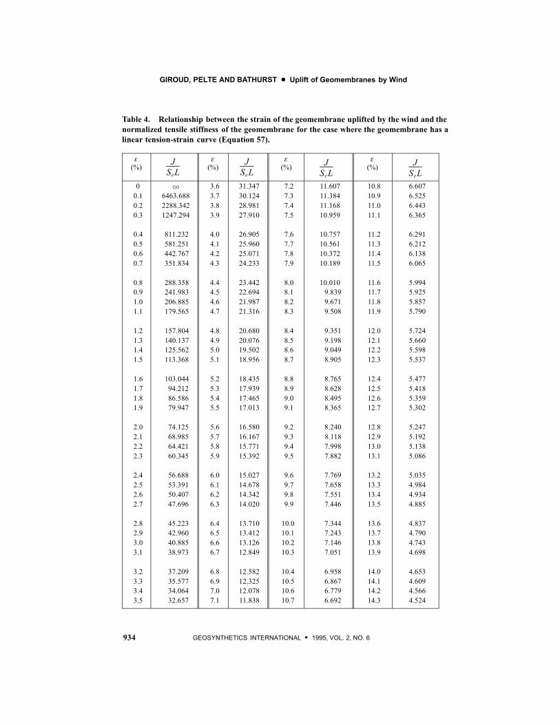
GIROUD, PELTE AND BATHURST D Uplift of Geomembranes by Wind
934 GEOSYNTHETICS INTERNATIONAL S 1995, VOL. 2, NO. 6
Table 4. Relationship between the strain of the geomembrane uplifted by the wind and the
normalized tensile stiffness of the geomembrane for the case where the geomembrane has a
linear tension-strain curve (Equation 57).
(%)
J
SeL
(%)
J
SeL
(%)
J
SeL
(%)
J
SeL
0
0.1
0.2
0.3
0.4
0.5
0.6
0.7
0.8
0.9
1.0
1.1
1.2
1.3
1.4
1.5
1.6
1.7
1.8
1.9
2.0
2.1
2.2
2.3
2.4
2.5
2.6
2.7
2.8
2.9
3.0
3.1
3.2
3.3
3.4
3.5
1
6463.688
2288.342
1247.294
811.232
581.251
442.767
351.834
288.358
241.983
206.885
179.565
157.804
140.137
125.562
113.368
103.044
94.212
86.586
79.947
74.125
68.985
64.421
60.345
56.688
53.391
50.407
47.696
45.223
42.960
40.885
38.973
37.209
35.577
34.064
32.657
3.6
3.7
3.8
3.9
4.0
4.1
4.2
4.3
4.4
4.5
4.6
4.7
4.8
4.9
5.0
5.1
5.2
5.3
5.4
5.5
5.6
5.7
5.8
5.9
6.0
6.1
6.2
6.3
6.4
6.5
6.6
6.7
6.8
6.9
7.0
7.1
31.347
30.124
28.981
27.910
26.905
25.960
25.071
24.233
23.442
22.694
21.987
21.316
20.680
20.076
19.502
18.956
18.435
17.939
17.465
17.013
16.580
16.167
15.771
15.392
15.027
14.678
14.342
14.020
13.710
13.412
13.126
12.849
12.582
12.325
12.078
11.838
7.2
7.3
7.4
7.5
7.6
7.7
7.8
7.9
8.0
8.1
8.2
8.3
8.4
8.5
8.6
8.7
8.8
8.9
9.0
9.1
9.2
9.3
9.4
9.5
9.6
9.7
9.8
9.9
10.0
10.1
10.2
10.3
10.4
10.5
10.6
10.7
11.607
11.384
11.168
10.959
10.757
10.561
10.372
10.189
10.010
9.839
9.671
9.508
9.351
9.198
9.049
8.905
8.765
8.628
8.495
8.365
8.240
8.118
7.998
7.882
7.769
7.658
7.551
7.446
7.344
7.243
7.146
7.051
6.958
6.867
6.779
6.692
10.8
10.9
11.0
11.1
11.2
11.3
11.4
11.5
11.6
11.7
11.8
11.9
12.0
12.1
12.2
12.3
12.4
12.5
12.6
12.7
12.8
12.9
13.0
13.1
13.2
13.3
13.4
13.5
13.6
13.7
13.8
13.9
14.0
14.1
14.2
14.3
6.607
6.525
6.443
6.365
6.291
6.212
6.138
6.065
5.994
5.925
5.857
5.790
5.724
5.660
5.598
5.537
5.477
5.418
5.359
5.302
5.247
5.192
5.138
5.086
5.035
4.984
4.934
4.885
4.837
4.790
4.743
4.698
4.653
4.609
4.566
4.524

GIROUD, PELTE AND BATHURST D Uplift of Geomembranes by Wind
935GEOSYNTHETICS INTERNATIONAL S 1995, VOL. 2, NO. 6
Table 4. (Continued)
(%)
J
SeL
(%)
J
SeL
(%)
J
SeL
(%)
J
SeL
14.4
14.5
14.6
14.7
14.8
14.9
15.0
15.1
15.2
15.3
15.4
15.5
15.6
15.7
15.8
15.9
16.0
16.1
16.2
16.3
16.4
16.5
16.6
16.7
16.8
16.9
17.0
17.1
17.2
17.3
17.4
17.5
17.6
17.7
17.8
17.9
4.482
4.441
4.400
4.361
4.322
4.283
4.246
4.209
4.172
4.136
4.101
4.066
4.031
3.998
3.964
3.932
3.900
3.868
3.836
3.806
3.776
3.745
3.716
3.687
3.658
3.630
3.602
3.575
3.548
3.521
3.495
3.469
3.444
3.418
3.393
3.369
18.0
18.1
18.2
18.3
18.4
18.5
18.6
18.7
18.8
18.9
19.0
19.1
19.2
19.3
19.4
19.5
19.6
19.7
19.8
19.9
20.0
20.1
20.2
20.3
20.4
20.5
20.6
20.7
20.8
20.9
21.0
21.1
21.2
21.3
21.4
21.5
3.345
3.321
3.297
3.274
3.251
3.229
3.206
3.184
3.163
3.141
3.120
3.099
3.078
3.058
3.038
3.018
2.998
2.979
2.960
2.941
2.922
2.905
2.885
2.867
2.849
2.832
2.814
2.797
2.780
2.763
2.747
2.730
2.714
2.698
2.682
2.666
21.6
21.7
21.8
21.9
22.0
22.1
22.2
22.3
22.4
22.5
22.6
22.7
22.8
22.9
23.0
23.1
23.2
23.3
23.4
23.5
23.6
23.7
23.8
23.9
24.0
24.1
24.2
24.3
24.4
24.5
24.6
24.7
24.8
24.9
25.0
25.1
2.651
2.635
2.620
2.605
2.590
2.576
2.561
2.547
2.532
2.518
2.504
2.491
2.477
2.464
2.450
2.437
2.424
2.411
2.399
2.386
2.373
2.361
2.348
2.336
2.324
2.312
2.301
2.289
2.278
2.266
2.255
2.243
2.232
2.221
2.210
2.199
25.2
25.3
25.4
25.5
25.6
25.7
25.8
25.9
26.0
26.1
26.2
26.3
26.4
26.5
26.6
26.7
26.8
26.9
27.0
27.1
27.2
27.3
27.4
27.5
27.6
27.7
27.8
27.9
28.0
28.1
28.2
28.3
28.4
28.5
28.6
28.7
2.189
2.178
2.168
2.157
2.147
2.137
2.127
2.117
2.107
2.097
2.087
2.077
2.068
2.059
2.049
2.040
2.031
2.021
2.012
2.003
1.994
1.986
1.977
1.968
1.960
1.951
1.943
1.934
1.926
1.918
1.910
1.902
1.894
1.886
1.878
1.870

GIROUD, PELTE AND BATHURST D Uplift of Geomembranes by Wind
936 GEOSYNTHETICS INTERNATIONAL S 1995, VOL. 2, NO. 6
Table 4. (Continued)
(%)
J
SeL
(%)
J
SeL
(%)
J
SeL
(%)
J
SeL
28.8
28.9
29.0
29.1
29.2
29.3
29.4
29.5
29.6
29.7
29.8
29.9
30.0
30.1
30.2
30.3
30.4
30.5
30.6
30.7
30.8
30.9
31.0
31.1
31.2
31.3
31.4
31.5
31.6
31.7
31.8
31.9
32.0
32.1
32.2
32.3
1.862
1.854
1.847
1.840
1.832
1.824
1.817
1.810
1.802
1.795
1.788
1.781
1.774
1.767
1.760
1.753
1.746
1.739
1.733
1.726
1.719
1.713
1.706
1.700
1.694
1.687
1.681
1.675
1.668
1.662
1.656
1.650
1.644
1.638
1.632
1.626
32.4
32.5
32.6
32.7
32.8
32.9
33.0
33.1
33.2
33.3
33.4
33.5
33.6
33.7
33.8
33.9
34.0
34.1
34.2
34.3
34.4
34.5
34.6
34.7
34.8
34.9
35.0
35.1
35.2
35.3
35.4
35.5
35.6
35.7
35.8
35.9
1.620
1.615
1.609
1.603
1.598
1.592
1.586
1.581
1.575
1.570
1.564
1.559
1.553
1.548
1.542
1.538
1.532
1.527
1.522
1.517
1.512
1.507
1.502
1.497
1.492
1.487
1.482
1.477
1.472
1.468
1.463
1.458
1.453
1.449
1.444
1.440
36.0
36.1
36.2
36.3
36.4
36.5
36.6
36.7
36.8
36.9
37.0
37.1
37.2
37.3
37.4
37.5
37.6
37.7
37.8
37.9
38.0
38.1
38.2
38.3
38.4
38.5
38.6
38.7
38.8
38.9
39.0
39.1
39.2
39.3
39.4
39.5
1.435
1.431
1.426
1.422
1.417
1.413
1.408
1.404
1.400
1.395
1.391
1.387
1.383
1.379
1.374
1.370
1.367
1.362
1.359
1.354
1.350
1.346
1.342
1.338
1.334
1.330
1.327
1.323
1.319
1.315
1.311
1.308
1.304
1.301
1.297
1.293
39.6
39.7
39.8
39.9
40.0
40.1
40.2
40.3
40.4
40.5
40.6
40.7
40.8
40.9
41.0
41.1
41.2
41.3
41.4
41.5
41.6
41.7
41.8
41.9
42.0
42.1
42.2
42.3
42.4
42.5
42.6
42.7
42.8
42.9
43.0
43.1
1.289
1.286
1.282
1.279
1.275
1.271
1.268
1.265
1.261
1.258
1.254
1.251
1.248
1.244
1.241
1.237
1.234
1.231
1.228
1.224
1.221
1.218
1.214
1.211
1.208
1.205
1.202
1.199
1.196
1.193
1.190
1.187
1.184
1.181
1.178
1.175

GIROUD, PELTE AND BATHURST D Uplift of Geomembranes by Wind
937GEOSYNTHETICS INTERNATIONAL S 1995, VOL. 2, NO. 6
Table 4. (Continued)
(%)
J
SeL
(%)
J
SeL
(%)
J
SeL
(%)
J
SeL
43.2
43.3
43.4
43.5
43.6
43.7
43.8
43.9
44.0
44.1
44.2
44.3
44.4
44.5
44.6
44.7
44.8
44.9
45.0
45.1
45.2
45.3
45.4
45.5
45.6
45.7
45.8
45.9
46.0
46.1
46.2
46.3
46.4
46.5
46.6
46.7
1.172
1.169
1.166
1.163
1.160
1.157
1.154
1.151
1.149
1.146
1.143
1.140
1.137
1.135
1.132
1.129
1.127
1.124
1.121
1.118
1.116
1.113
1.111
1.108
1.105
1.103
1.100
1.098
1.095
1.093
1.090
1.088
1.085
1.082
1.080
1.078
46.8
46.9
47.0
47.1
47.2
47.3
47.4
47.5
47.6
47.7
47.8
47.9
48.0
48.1
48.2
48.3
48.4
48.5
48.6
48.7
48.8
48.9
49.0
49.1
49.2
49.3
49.4
49.5
49.6
49.7
49.8
49.9
50.0
50.1
50.2
50.3
1.075
1.073
1.070
1.068
1.065
1.063
1.061
1.058
1.056
1.054
1.051
1.049
1.047
1.044
1.042
1.040
1.038
1.035
1.033
1.031
1.029
1.026
1.024
1.022
1.020
1.018
1.016
1.013
1.011
1.009
1.007
1.005
1.003
1.001
0.999
0.997
50.4
50.5
50.6
50.7
50.8
50.9
51.0
51.1
51.2
51.3
51.4
51.5
51.6
51.7
51.8
51.9
52.0
52.1
52.2
52.3
52.4
52.5
52.6
52.7
52.8
52.9
53.0
53.1
53.2
53.3
53.4
53.5
53.6
53.7
53.8
53.9
0.995
0.992
0.990
0.989
0.986
0.984
0.982
0.980
0.978
0.976
0.974
0.973
0.971
0.969
0.967
0.965
0.963
0.961
0.959
0.957
0.955
0.953
0.952
0.950
0.948
0.946
0.944
0.942
0.941
0.939
0.937
0.935
0.933
0.932
0.930
0.928
54.0
54.1
54.2
54.3
54.4
54.5
54.6
54.7
54.8
54.9
55.0
55.1
55.2
55.3
55.4
55.5
55.6
55.7
55.8
55.9
56.0
56.1
56.2
56.3
56.4
56.5
56.6
56.7
56.8
56.9
57.0
57.08
0.926
0.925
0.923
0.921
0.919
0.918
0.916
0.914
0.913
0.911
0.909
0.908
0.906
0.904
0.903
0.901
0.899
0.898
0.896
0.895
0.893
0.891
0.890
0.888
0.887
0.885
0.883
0.882
0.880
0.879
0.877
0.876
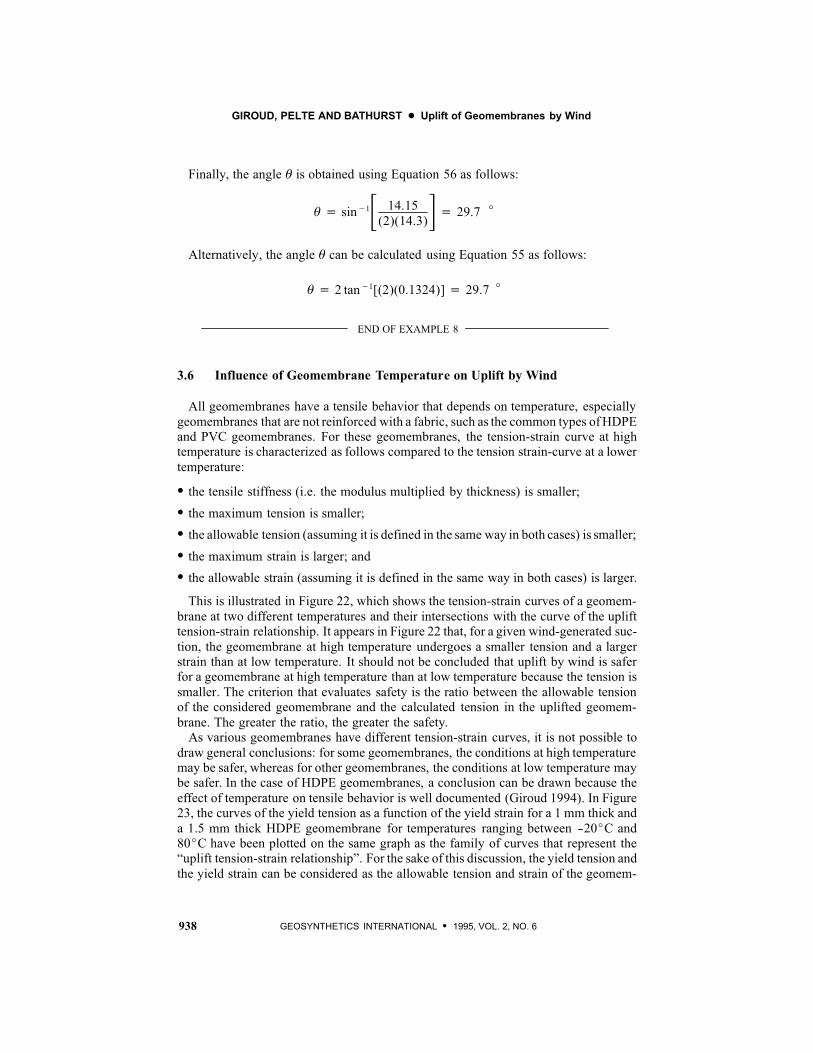
GIROUD, PELTE AND BATHURST D Uplift of Geomembranes by Wind
938 GEOSYNTHETICS INTERNATIONAL S 1995, VOL. 2, NO. 6
Finally, the angle $ is obtained using Equation 56 as follows:
$ sin"1% 14.15(2)(14.3)& 29.7 _
Alternatively, the angle $ can be calculated using Equation 55 as follows:
$ 2 tan"1[(2)(0.1324)] 29.7 _
END OF EXAMPLE 8
3.6 Influence of Geomembrane Temperature on Uplift by Wind
All geomembranes have a tensile behavior that depends on temperature, especially
geomembranes that are not reinforced with a fabric, such as the common types ofHDPEand PVC geomembranes. For these geomembranes, the tension-strain curve at hightemperature is characterized as follows compared to the tension strain-curve at a lower
temperature:
S the tensile stiffness (i.e. the modulus multiplied by thickness) is smaller;
S the maximum tension is smaller;
S the allowable tension (assuming it is defined in the same way in both cases) is smaller;
S the maximum strain is larger; and
S the allowable strain (assuming it is defined in the same way in both cases) is larger.
This is illustrated in Figure 22, which shows the tension-strain curves of a geomem-
brane at two different temperatures and their intersections with the curve of the uplifttension-strain relationship. It appears in Figure 22 that, for a given wind-generated suc-
tion, the geomembrane at high temperature undergoes a smaller tension and a largerstrain than at low temperature. It should not be concluded that uplift by wind is saferfor a geomembrane at high temperature than at low temperature because the tension is
smaller. The criterion that evaluates safety is the ratio between the allowable tensionof the considered geomembrane and the calculated tension in the uplifted geomem-
brane. The greater the ratio, the greater the safety.As various geomembranes have different tension-strain curves, it is not possible to
draw general conclusions: for some geomembranes, the conditions at high temperaturemay be safer, whereas for other geomembranes, the conditions at low temperature maybe safer. In the case of HDPE geomembranes, a conclusion can be drawn because the
effect of temperature on tensile behavior is well documented (Giroud 1994). In Figure23, the curves of the yield tension as a function of the yield strain for a 1 mm thick and
a 1.5 mm thick HDPE geomembrane for temperatures ranging between --20_C and80_C have been plotted on the same graph as the family of curves that represent the“uplift tension-strain relationship”. For the sake of this discussion, the yield tension and
the yield strain can be considered as the allowable tension and strain of the geomem-

GIROUD, PELTE AND BATHURST D Uplift of Geomembranes by Wind
939GEOSYNTHETICS INTERNATIONAL S 1995, VOL. 2, NO. 6
Figure 22. Influence of geomembrane temperature on the tension and strain of the uplifted
geomembrane.
Figure23. Curves representing a typical relationship between yield tension and yield strain
of 1.0 and1.5mmthickHDPEgeomembranes (fromGiroud1994) plotted on the samegraph
as the family of curves representing the uplift tension-strain relationship (from Figure 13).
Geomembrane strain, (%)
Geomembranetension,(kN/m)
T
tGM = 1.5 mm
tGM = 1 mm
Value of Se L (kN/m) along each curve
SeL
Geomembranetemperature(_C)

GIROUD, PELTE AND BATHURST D Uplift of Geomembranes by Wind
940 GEOSYNTHETICS INTERNATIONAL S 1995, VOL. 2, NO. 6
brane. It appears clearly in Figure 23 that HDPE geomembranes better resist wind upliftat low temperatures than at high temperatures. For example, a 1 mm thick HDPE geo-membrane would reach yield in a situation characterized by a Se L value of approxi-
mately 30 kN/m at 0_C and 20 kN/m at 60_C. Therefore, when evaluating the upliftresistance of an HDPE geomembrane, the highest possible temperature should be con-
sidered to calculate the factor of safety conservatively. However, the lowest possibletemperature should also be considered because, in this case, the tension in the uplifted
geomembrane has its highest value, which should be used for anchor trench design.It should also be noted that, in actual design situations, the comparison between geo-
membrane uplift at high and low temperature is complicated by the fact that wind veloc-
ity is often different in the winter and in the summer. This situation is illustrated in Ex-ample 9.
Example 9. A geomembrane, with a mass per unit area of 1.8 kg/m2, installed in areservoir located at the sea level is exposed to a wind velocity of 90 km/h in the winter
and 140 km/h in the summer. Typical temperatures of the geomembrane when the windblows are 0_C in the winter and 50_C in the summer. The tension-strain curve of the
geomembrane is assumed to be linear with a tensile stiffness of 900 kN/m at 0_C and400 kN/m at 50_C. What is the geomembrane tension on slopes that are 17 m long?
First, the situation in the winter is considered. Equation 39 gives the effective suctionas follows:
Se (0.05)(0.7)(902)! (9.81)(1.8) 283.5! 17.7 265.8 Pa
hence:
SeL (265.8)(17) 4519 N"m 4.52 kN"m
Then, the normalized tensile stiffness is obtained as follows:
J
SeL 9004.52
199.1
For J/(Se L) = 199, Table 4 gives = 1.0%. Then Equation 34 gives:
T = (0.010) (900) = 9.0 kN/m
Then it is useful to calculate ! to have the orientation of the tension T, which is neces-sary to design the anchor trench. The angle ! is calculated as follows using Equation56:
! sin!1# 4.52(2)(9.0)$ 14.5 _

GIROUD, PELTE AND BATHURST D Uplift of Geomembranes by Wind
941GEOSYNTHETICS INTERNATIONAL S 1995, VOL. 2, NO. 6
Second, the situation in the summer is considered. Equation 39 gives the effectivesuction as follows:
Se (0.05)(0.7)(1402)! (9.81)(1.8) 686.0! 17.7 668.3 Pa
hence:
SeL (668.3)(17) 11, 361 N"m 11.36 kN"m
Then, the normalized tensile stiffness is obtained as follows:
J
SeL 40011.36
35.2
For J/(Se L) = 35, Table 4 gives = 3.3%. Then Equation 34 gives:
T = (0.033)(400) = 13.2 kN/m
It appears that the tension is greater in the summer than in the winter. This is becausethe higher wind velocity in the summer has overcome the effect of the higher geomem-
brane stiffness in the winter. This is illustrated in Figure 24.The orientation, !, of the tension is then calculated as follows using Equation 56:
! sin!1# 11.4
(2)(13.2)$ 25.6 _
END OF EXAMPLE 9
In all the calculations and discussions presented in Section 3, it has been implicitlyassumed that the geomembrane has no wrinkles and no tension just before wind uplift
occurs. In reality, at high temperature, the geomembrane may exhibit wrinkles and, atlow temperature, the geomembrane may be under tension as a result of restrained con-
traction. Both cases can easily be addressed bymoving the geomembrane tension-straincurve laterally by an amount T , which is the thermal contraction or expansion of thegeomembrane calculated as follows:
ÁT "(#! #base) (58)
where: " = coefficient of thermal expansion-contraction of the geomembrane; # = tem-perature of the geomembrane when uplift occurs; and #base = temperature of the geo-membrane when it rests on the supporting groundwithout wrinkles and without tension.(This case is referred to as the base case hereinafter.)

GIROUD, PELTE AND BATHURST D Uplift of Geomembranes by Wind
942 GEOSYNTHETICS INTERNATIONAL S 1995, VOL. 2, NO. 6
Figure 24. Illustration of Example 9.
(Notes: The curves are as follows: straight lines for the geomembrane tension-strain curve at 0_C (Curve
0_) and at 50_C (Curve 50_); curves representing the uplift tension-strain relationship for a wind velocity of
90 km/h in the winter (Curve W) and for a wind velocity of 140 km/h in the summer (Curve S).)
Geomembrane strain, (%)
Geomembranetension,(kN/m)
T
(0_)
(50_)
(S)
(W)
The foregoing discussion is illustrated in Figure 25 which shows the following:
S If the geomembrane has wrinkles when uplifting begins, its behavior is represented
by Curve 1 (i.e. T > 0 because # > #base). The figure shows that, for a given value ofSeL, the apparent strain, app1 , in the uplifted geomembrane is greater than the strain, base , in the uplifted geomembrane for the base case where the geomembrane has nowrinkles or tension when uplifting begins (i.e. app1 > base). Since the geometry of theuplifted geomembrane (u, !) is governed by the apparent strain, a geomembrane isuplifted more (i.e. u and ! are larger) if it has wrinkles at the beginning of upliftingthan if it has no wrinkles. The figure also shows that the tension in the uplifted geo-membrane, T1 , is less than it would be in the base case where the geomembrane has
no wrinkles or tension when uplifting begins (i.e. T1 < Tbase). The tension, T1 corre-sponds to an actual strain 1 = app1 -- T < base . In summary, if a geomembrane haswrinkles when uplifting begins, it is uplifted more, but with a smaller tension, thanif the geomembrane has no wrinkles when uplifting begins.
S If the geomembrane is under tension when uplifting begins, its behavior is repre-
sented by Curve 2 (i.e. T < 0 because # < #base). The figure shows that, for a givenvalue of SeL, the apparent strain, app2 , in the uplifted geomembrane is less than thestrain, base , in the uplifted geomembrane for the base case where the geomembranehas no tension or wrinkles when uplifting begins (i.e. app2 < base). Since the geometry

GIROUD, PELTE AND BATHURST D Uplift of Geomembranes by Wind
943GEOSYNTHETICS INTERNATIONAL S 1995, VOL. 2, NO. 6
Figure 25. Uplift by the wind of a geomembrane with wrinkles at high temperature (Curve
1) and tension before uplift at low temperature (Curve 2).
Geomembranetension-strain curve
Curve of the uplift tension-strain relationship for theconsidered value of SeL
(Note: Both Curves 1 and 2 are derived from the geomembrane tension-strain curve by translation parallel
to the O axis.)
T > 0 T < 0
Thermal expansion (wrinkles before uplift)
Thermal contraction (tension before uplift)
T2
T1
Tbase
app2 app1
base
of the uplifted geomembrane (u, !) is governed by the apparent strain, a geomem-brane is uplifted less (i.e. u and ! are less) if it is under tension when uplifting beginsthan if it is not. The figure also shows that the tension in the uplifted geomembrane,
T2 , is greater than it would be in the base case where the geomembrane has no tensionor wrinkles when uplifting begins (i.e. T2 > Tbase). The tension, T2 corresponds to an
actual strain 2= app2 -- T = app2 + | T | > base . In summary, if a geomembrane is undertension when uplifting begins, it is uplifted less, but with a greater tension, than if the
geomembrane is not under tension when uplifting begins.
4 PRACTICAL RECOMMENDATIONS
4.1 Recommendations for Preventing Geomembrane Uplift
From the above discussions and design examples, it appears that geomembranes,
even those that are heavy, can be significantly uplifted by the wind and can be damagedas explained in Section 1. It is therefore important to try to prevent uplift of geomem-
branes by wind.

GIROUD, PELTE AND BATHURST D Uplift of Geomembranes by Wind
944 GEOSYNTHETICS INTERNATIONAL S 1995, VOL. 2, NO. 6
4.1.1 Protective Cover
A layer of heavy material, such as soil (assuming it is not removed by the wind), con-crete, or equivalent, covering the entire geomembrane, or certain parts most likely tobe uplifted, is an effective preventive measure. Equations have been provided in Sec-
tion 2.4 to calculate the required thickness of such protective covers. Examples haveshown that a thickness of a few centimeters is generally sufficient.
4.1.2 Impounded Liquid
A rather small depth of liquid, at the bottom of a reservoir, can prevent geomembraneuplift. Equations have been provided in Section 2.4 to calculate the required depth of
liquid (typically 100 to 300 mm). A factor of safety is recommended because the windmay displace the liquid and locally decrease the depth of liquid.
4.1.3 Sandbags
Sandbags are only effective for winds with a rather small velocity. It has been shownin Section 2.4 that, to ensure uplift prevention in case of high-velocity winds, the num-
ber of sandbags would be prohibitive. Also, sandbags can be harmful to the geomem-brane for the case of high-velocity winds because they can be displaced when the geo-
membrane is uplifted and could damage the geomembrane as they move. Sandbags aremost effective during construction to prevent the geomembrane from being displacedby low-velocity winds. It is more effective to use a line of adjacent sandbags along the
edge of the geomembrane panel just installed than to scatter the sandbags on theinstalled geomembrane; calculations presented in this paper have shown that scattered
sandbags are not very effective, whereas a line of adjacent sandbags at the edge of theinstalled geomembrane prevents air from flowing under the geomembrane, a major
cause of geomembrane uplift.
4.1.4 Suction Vents
Suction vents located at the top of slopes are generally believed to be an effective way
to prevent or reduce uplift of a geomembrane by the wind. These vents stabilize the geo-membrane by sucking air from beneath the geomembrane when the wind blows, there-by decreasing the air pressure beneath the geomembrane. For the suction vents to work,
air located beneath the geomembrane must flow toward the vent when the air vent isexposed to wind-generated suction. If the soil beneath the geomembrane has a low
permeability, there is little air beneath the geomembrane. This air will flow toward thevent after the geomembrane has been slightly uplifted. If the soil beneath the geomem-
brane is permeable there is a significant amount of air entrapped beneath the geomem-brane, and while this air is being sucked out by the suction vent, the geomembrane isuplifted. Therefore, in all cases the geomembrane may be uplifted for a short period of
time before the suction vents are effective. In cases where the soil beneath the geomem-brane has a low permeability, short strips of drainage geocomposites, radiating from the
suction vent, have been recommended to help drain the air located beneath the geo-membrane. However, the effectiveness of this method has not been evaluated.

GIROUD, PELTE AND BATHURST D Uplift of Geomembranes by Wind
945GEOSYNTHETICS INTERNATIONAL S 1995, VOL. 2, NO. 6
To the best of the authors’ knowledge, nomethod is available to design suction vents.Ideally, the design of suction vents should address the following: size and configurationof the vent; spacing between vents; and required permeability of the material located
beneath the geomembrane. The only point that is well established is that the vents mustbe at the crest or, at the top of the slope near the crest, in accordance with the data pres-
ented in Section 2.2. In a number of projects, suction vents have been placed every 15m along the periphery of ponds. The reason for selecting 15 m as the spacing is not
known. The shape of the suction vents should be such that precipitation water and runoffwater are prevented from entering the vent.
4.1.5 Plastic Tubes and Sandbags Associated with Suction Vents
Sand-filled plastic tubes or rows of sandbags running from the crest to the toe ofslopes are sometimes proposed in conjunction with suction vents. This is a logical com-bination because sandbags or sand-filled tubes are most effective in case of low-veloc-
ity winds and are effective without any delay, whereas suction vents (which are general-ly considered to be effective at any wind velocity) require some time to be effective,
as explained above. It is important to make sure that the tubes or the row of bags do nothamper circulation of air beneath the geomembrane, which is required for the function-
ing of the suction vents. Therefore such tubes or rows of sandbags should be placed mid-way between two consecutive suction vents and, if it has been determined that suctionvents are necessary, there should not be two parallel tubes or rows of adjacent sandbags
without a suction vent in between.
4.1.6 Vacuum
Geomembranes used as landfill covers are rarely left exposed. However, such a de-
sign may be considered in areas where the use of an exposed geomembrane is aestheti-cally acceptable and if precautions are taken to ensure that the geomembrane is not
damaged by the wind.The suction exerted by the wind on a landfill may be calculated using Equation 37
with the values of $ summarized in Figure 5, which were initially established for struc-tures associated with reservoirs. However, consistent with recommendations made inSection 2.2, values of $ increased by up to 30% or additional studies, such as wind-tun-nel tests of reduced-scale models and numerical simulations, may be warranted in thecase of landfills that have an unusual shape.
The use of suction vents to prevent geomembrane uplift by wind is not recommendedin the case of a landfill because such vents may promote the infiltration of air into thelandfill, which is undesirable because oxygen: inhibits the anaerobic process of waste
decomposition; may promote fires in the waste; and may, under certain conditions,create an explosive mixture with methane. Some landfills are equipped with an active
gas collection system to collect the methane generated as a result of anaerobic decom-position of the waste. These active gas collection systems comprise blowers that main-
tain a vacuum in a network of perforated pipes located in the waste. Typically, the mag-nitude of the vacuum is on the order of 10 kPa at the blower and is less throughout thenetwork of perforated pipes. Active gas collection systems are typically not designed
to apply any significant vacuum immediately beneath the landfill cover system, in order

GIROUD, PELTE AND BATHURST D Uplift of Geomembranes by Wind
946 GEOSYNTHETICS INTERNATIONAL S 1995, VOL. 2, NO. 6
to minimize the risk of air infiltration into the landfill. However, it should be possibleto modify an active gas collection system to apply a small vacuum (such as 1 to 2 kPa,according to Figure 3) beneath the geomembrane to prevent geomembrane uplift by the
wind. This could be achieved by placing some of the perforated pipes relatively closeto the geomembrane cover. These pipes, would mostly be dedicated to the prevention
of geomembrane uplift, and would only be activated when the wind starts blowing. Thevacuum system should be designed so that the required vacuum (e.g. 2 kPa) can be es-
tablished beneath the geomembrane before the wind velocity reaches its maximum val-ue. It is important that the blowers for the pipe network dedicated to geomembraneuplift prevention be supplied with electricity regardless of wind velocity, even though
high-velocity windsmay cause power outages; this could be achieved with awind-pow-ered electricity generator. It is also advisable to ensure a permanent supply of electrical
power to the blowers of the main pipe network, i.e. the network dedicated to gas collec-tion, because the pipes dedicated to geomembrane uplift prevention may not be fullyeffective if the gas collection system is not operating at the same time.
4.2 Recommendations for the Case of Exposed Geomembranes
When geomembranes are exposed, i.e. not covered with a protective layer, they are
likely to be uplifted by the wind. In Section 2.3, equations are provided that give thethreshold wind velocity beyond which a given geomembrane is uplifted depending onthe geomembrane mass per unit area, the location of the considered portion of geomem-
brane in the facility, and the altitude above sea level. The large tensions generated inthe uplifted geomembrane are transmitted to the anchor trenches. It is important that
the anchor trenches be designed to accommodate these large tensions. The design ofanchor trenches is beyond the scope of this paper. However, the method presented inthis paper provides two essential types of data for the design of anchor trenches: the ten-
sion, T, in the geomembrane, i.e. the tension exerted by the geomembrane on its anchortrench; and the orientation, !, of the tension T.Intermediate benches or anchor trenches (Figures 7c and 7d) are very effective be-
cause they decrease the length of free geomembrane subjected to wind suction. Since
wind-generated suction is larger in the upper portion of a slope than in the lower portion(see Figure 5), benches or anchor trenches should be more closely spaced in the upperportion of the slope than in the lower portion. Ideal spacings are shown in Figure 26.
These spacings are such that the product of the spacing and the suction factor, $, is aconstant. A remarkable example of such a design is Barlovento reservoir, constructed
in 1991-1992 in a large crater (600 m diameter) in the Canary Islands, Spain (Fayoux1992, 1993) (Figure 27) at an altitude of 700 m. A similar design had been done by thesenior author in 1977 for another crater reservoir, also in the Canary Islands, but not yet
constructed. The side slope of the Barlovento reservoir is 1V:2.75H and is 30 m high.In the first phase, only the bottom and the lower 20 m of the side slope were lined, using
a 1.5 mm thick PVC geomembrane reinforced with a polyester scrim on the side slopeand a 1.5 mm thick unreinforced PVC geomembrane on the bottom. As seen in Figure
27, because of the spiral shape of the anchor trenches, the number of anchor trenchesat a given location along the slope is either three or four, in addition to one anchor trenchat the top of the lined portion of the slope and one anchor trench at the toe of the slope.

GIROUD, PELTE AND BATHURST D Uplift of Geomembranes by Wind
947GEOSYNTHETICS INTERNATIONAL S 1995, VOL. 2, NO. 6
Figure 26. Ideal spacing for anchor trenches or benches on a slope: (a) two spacings;
(b) three spacings.
(a)
(b)
Figure 27. Barlovento reservoir in the Canary Islands (courtesy of D. Fayoux).
(Notes: Three stages of construction are seen on this photograph: 1) in the right part of the photograph, the
four intermediate anchor trenches are visible; 2) in the center-right of the photograph, which appears almost
identical to the right part, a layer of porous concrete has been placed on the slope and the geomembrane tabs
(which are anchored in the anchor trenches and pass through the porous concrete) are visible; and 3) on the
left half of the photograph, the white PVC geomembrane has been placed and seamed to the tabs. It should
be noted that the anchor trenches are not horizontal, but form a spiral at the periphery because they contain
a drain with a 1% slope.)

GIROUD, PELTE AND BATHURST D Uplift of Geomembranes by Wind
948 GEOSYNTHETICS INTERNATIONAL S 1995, VOL. 2, NO. 6
Figure 28. Additional soil mass at toe of slope to resist localized uplift of geomembrane at
bottom due to tension in geomembrane on slope.
The distances measured along the slope between the anchor trenches located on theslope are, from top to bottom: 14.1 m, 15.2 m, and 18.8 m.As indicated in Section 4.1, a relatively thin soil layer is sufficient to prevent geo-
membrane uplift at the bottom of a pond. However, this thin soil layer may not be suffi-cient as an “anchorage” to resist localized uplift due to the tension of the uplifted geo-
membrane at the toe of the slope. Therefore, an additional soil mass at the toe of theslope is required, as shown in Figure 28.
As indicated in Section 4.1, suction vents are generally believed to be an effectiveway to prevent or reduce uplift by the wind of exposed geomembranes located on aslope. Therefore, suction vents should be considered every time the slopes of a geo-
membrane-lined facility are expected to be exposed to high-velocity winds and cannotbe covered with a protective layer for any reasons such as stability or cost. However,
it is hard to find documented information on the performance of suction vents and a de-sign method needs to be developed.
5 CONCLUSIONS
The detailed analysis of the phenomenon of uplift of geomembranes by wind pres-ented in this paper has yielded the following results:
S The uplift effect of wind on geomembranes depends on wind velocity, altitude above
sea level, and location of the geomembrane in the considered facility (e.g. the geo-
membrane is more likely to be uplifted if it is at the crest of a dike than on a side slope,andmore likely to be uplifted on a side slope than at the bottom). Equations were pro-vided to calculate the wind-generated suction as a function of these parameters.
S Whether or not a geomembrane will be uplifted by the wind depends on the above
parameters and on the mass per unit area of the geomembrane. At a given location,
the threshold wind velocity at which a geomembrane starts being uplifted is higherfor a heavy geomembrane (such as a bituminous geomembrane) than for a light geo-
membrane (such as a polymeric geomembrane). Equations were provided to calcu-late threshold wind velocities.
S When a geomembrane is uplifted, its tension, strain, and deformation depend on its
tensile characteristics. Equations, tables and graphical methods were provided to de-

GIROUD, PELTE AND BATHURST D Uplift of Geomembranes by Wind
949GEOSYNTHETICS INTERNATIONAL S 1995, VOL. 2, NO. 6
termine the tension, strain and geometry of uplifted geomembranes as a function ofwind velocity, altitude above sea level, location of the geomembrane in the consid-ered facility, and tensile characteristics of the geomembrane. Geomembranes with a
high tensile stiffness (i.e. high modulus) deform less than geomembranes with a lowtensile stiffness, but they undergo a greater tension and apply a greater pullout force
on anchor trenches.
S The condition of the geomembrane when uplifting begins has a significant influence
on the magnitude of uplifting and the condition of the uplifted geomembrane. If ageomembrane has wrinkles when uplifting begins, it is uplifted more, but with asmaller tension than if the geomembrane has no wrinkles when uplifting begins. If
a geomembrane is under tension when uplifting begins, it is uplifted less, but with agreater tension than if the geomembrane is not under tension when uplifting begins.
S Since temperature has a significant effect on the tensile characteristics of geomem-
branes, the effect of temperature on geomembrane uplift by wind has been analyzed.
At a given location and for a given wind velocity, a given geomembrane will exhibitless strain but more tension at low temperature than at high temperature. The method
presented in this paper allows the designer to quantify the effect of temperature onwind uplift. It has been shown that HDPE geomembranes resist wind uplift better atlow temperature than at high temperature (i.e. the factor of safety based on allowable
tension and strain is greater at low than at high temperature).
S The most effective way to prevent the wind from uplifting geomembranes is to place
a protective cover on the geomembrane. Typical protective covers consist of a layerof soil or rock, concrete slabs or pavers, and bituminous revetments. A method has
been provided to determine the required thickness of the protective cover. Examplespresented in the paper show that a few centimeters are generally sufficient.
S Liquid stored in a pond is an effective way to prevent the wind from uplifting the geo-
membrane at the bottom of a pond. Equations which allow the determination of therequired depth of liquid are presented in the paper.
S Sandbags scattered on the geomembrane are only efficient to prevent geomembrane
uplift by low-velocity winds. The best way to use sandbags, during construction, is
to place a continuous row of sandbags at the edge of the installed portion of the geo-membrane to prevent the wind from getting under the geomembrane.
S Suction vents are based on a sound concept and they are believed to be effective in
preventing the wind from uplifting geomembranes or in reducing the magnitude ofgeomembrane uplift. However, to the best of the authors’ knowledge, there is no
method available for the design of suction vents, and there is little information ontheir performance. A variation of the suction vent strategy for landfill covers is to
modify the active gas collection system, if present, so that the blowers apply a smallsuction directly beneath the geomembrane cover to prevent uplift by wind.
The methods proposed in this paper are presented in a way that should be convenient
for design engineers, i.e. with equations, tables, graphical solutions and numerous de-sign examples. The senior author has used these methods, or previous versions of thesemethods, for the design of a number of geomembrane-lined structures since the early
1970s.

GIROUD, PELTE AND BATHURST D Uplift of Geomembranes by Wind
950 GEOSYNTHETICS INTERNATIONAL S 1995, VOL. 2, NO. 6
ACKNOWLEDGMENTS
The authors are pleased to acknowledge D. Fayoux of Groupe Solvay, Belgium, forthe valuable information he provided on the Barlovento reservoir and for thephotograph in Figure 27. The authors are also pleased to acknowledge B. Clark for the
valuable information she provided on landfill gas collection. The authors are gratefulto M.V. Khire for his review of the paper and to G. Saunders, A. Mozzar, S.M. Berdy
and K. Labinaz for their assistance in the preparation of the paper. Furthermore, the se-nior author is pleased to acknowledge the information and support provided by P. Huot
in the 1970s.
REFERENCES
Dedrick, A.R., 1973, “Air Pressures over Reservoir, Canal, and Water Catchment Sur-
faces Exposed toWind”, Ph.D. Thesis, Utah State University, Logan, Utah, USA, 189p.
Dedrick, A.R., 1974a, “Air Pressures over Surfaces Exposed toWind. WaterHarvestingCatchments”, Transactions of the ASAE, Vol. 17, No. 5, pp. 917-921.
Dedrick, A.R., 1974b, “Aerodynamic PressureDistributions over Reservoir, Canal, and
Water Catchment Surfaces Exposed to Wind”, Proceedings of the 6th InternationalColloquium on Plastics in Agriculture”, Vol. 1, Buenos Aires, Argentina, September1974, pp. 207-211.
Dedrick, A.R., 1975, “Air Pressures over Surfaces Exposed to Wind. Reservoirs”,Transactions of the ASAE, Vol. 18, No. 3, pp. 508-513.
Fayoux, D., 1992, “Use of PVC Geomembranes for Large Irrigation Works”, Proceed-
ings of XII Congreso Internacional de Plasticos en Agricultura, Granada, Spain, May1992, pp. I-43 - I-46.
Fayoux, D., 1993, “Le Bassin de Barlovento, The Barlovento Reservoir”, Proceedings
of Rencontres ’93, French Committee of Geotextiles and Geomembranes, Confer-ence held in Tours, France, September 1993, Vol. 2, pp. 365-374. (in French andEng-
lish)
Giroud, J.P., 1977, “Conception de l’étanchéité des ouvrages hydrauliques par géo-membranes”, Proceedings of the First International Symposium on Plastic and Rub-
ber Waterproofing in Civil Engineering, Vol. 1, Session 3, Paper 13, Liège, Belgium,June 1977, pp. III 13.1-III 13.17. (in French)
Giroud, J.P. and Huot, P., 1977, “Conception des barrages en terre et en enrochements
munis d’étanchéité par feuille mince”, Proceedings of the 11th Conference Euro-péenne de laCommission Internationale de l’Irrigation et duDrainage, CIID, Theme
3, Rome, Italy, May 1977, 8 p. (in French)
Giroud, J.P., 1994, “Quantification of Geosynthetics Behavior”, Proceedings of the 5thInternational Conference on Geotextiles, Geomembranes and Related Products, Vol.
4, Singapore, September 1994, pp. 1249-1273.
Goldstein, S., 1938, “Modern Developments in Fluid Dynamics”, Vol. 2, Oxford Engi-neering Science Series, Oxford University Press, United Kingdom, 702 p.

GIROUD, PELTE AND BATHURST D Uplift of Geomembranes by Wind
951GEOSYNTHETICS INTERNATIONAL S 1995, VOL. 2, NO. 6
Soderman, K.L. and Giroud, J.P., 1995, “Relationships Between Uniaxial and BiaxialStresses and Strains in Geosynthetics”, Geosynthetics International, Vol. 2, No. 2, pp.495-504.
The U.S. Standard Atmosphere, 1976, U.S. Government Printing Office, Washington,D.C., USA.
NOTATIONS
Basic SI units are given in parentheses.
A = area of a geomembrane (m2)
D = thickness of protective layer (m)
Dreq = required depth of protective layer (m)
F = force applied on geomembrane by uplift suction (defined in
Equation 42) (kN/m)
g = acceleration due to gravity (m/s2)
J = geomembrane tensile stiffness (N/m)
L = length of geomembrane subjected to suction (m)
Lmin = minimum value of L (m)
Lmax = maximum value of L (m)
p = atmospheric pressure at altitude z above sea level (Pa)
po = atmospheric pressure at sea level (Pa)
R = radius of circular-shaped uplifted geomembrane (m)
S = suction (Pa)
Se = “effective suction” defined by Equation 35 (Pa)
T = geomembrane tension (N/m)
Tall = allowable tension (N/m)
T%all
= normalized allowable tension as defined by Equation 48 (N/m)
Tbase = tension in an uplifted geomembrane for the base case where thegeomembrane has no wrinkles and no tension when uplifting begins
(N/m)
T1 = tension in an uplifted geomembrane that had wrinkles when upliftingbegan (N/m)
T2 = tension in an uplifted geomembrane that was under tension when
uplifting began (N/m)
tGM = thickness of the geomembrane (m)
u = geomembrane uplift (m)
V = wind velocity (m/s)
Vup = wind velocity that causes geomembrane uplift (m/s)
GIROUD, PELTE AND BATHURST D Uplift of Geomembranes by Wind
952 GEOSYNTHETICS INTERNATIONAL S 1995, VOL. 2, NO. 6
Vupmin = minimum value of Vup (m/s)
W = weight of a geomembrane (N)
z = altitude above sea level (m)
" = coefficient of thermal expansion-contraction of the geomembrane (_C-1)
% = lapse rate (_K/m)
# = temperature of the geomembrane when uplift occurs (_C)
#base = temperature of the geomembrane when it rests on the supporting groundwithout wrinkles and without tension (_C)
#0 = standard air temperature at sea level (_K)
pR = reference pressure variation (Pa)
= geomembrane strain (dimensionless)
all = allowable strain (dimensionless)
app = apparent strain of geomembrane (dimensionless)
app1 = apparent strain in an uplifted geomembrane that had wrinkles whenuplifting began (dimensionless)
app2 = apparent strain in an uplifted geomembrane that was under tension when
uplifting began (dimensionless)
base = strain in an uplifted geomembrane for the base case where thegeomembrane has no wrinkles and no tension when uplifting begins
(dimensionless)
T = thermal contraction or expansion as defined by Equation 58
(dimensionless)
! = angle between the extremities of the geomembrane and the straight linepassing through these extremities (_)
$ = suction factor defined by Equation 13 (dimensionless)
&GM = mass per unit area of the geomembrane (kg/m2)
&GMreq = mass per unit area of the geomembrane required to resist wind uplift(kg/m2)
' = air density (kg/m3)
'GM = density of the geomembrane (kg/m3)
'o = air density at sea level (kg/m3)
'P = density of the protective layer material (kg/m3)

187GEOSYNTHETICS INTERNATIONAL S 1997, VOL. 4, NO. 2
Technical Note by J.G. Zornberg and J.P. Giroud
UPLIFT OF GEOMEMBRANES BYWIND -
EXTENSION OF EQUATIONS
ABSTRACT: This technical note presents an extension of earlier analytical methods
published in 1995 by Giroud et al. for evaluating the uplift of geomembranes by wind.The extension incorporates: (i) the influence on wind uplift of the slope inclination ofan exposed geomembrane; and (ii) amore accurate expression of the tension-strain rela-
tionship in a wind uplifted geomembrane. Use of the revised methods is particularlyrelevant for projects in which the exposed geomembrane mass per unit area is high, the
slope inclination of the exposed geomembrane is steep, and the exposed geomembraneis subjected to strains due to mechanisms other than the wind (e.g. gravity, temperature)prior to wind uplift. Also, the revised equations are particularly appropriate for dimen-
sioning a protective layer placed on top of the geomembrane to prevent wind uplift. Theinformation provided in this technical note may be of particular significance for pro-
jects in which an exposed geomembrane is contemplated as the final cover for wastecontainment systems with steep slope configurations.
KEYWORDS: Geomembrane, Wind, Uplift, Design method, Steep slope.
AUTHORS: J.G. Zornberg, Assistant Project Engineer, GeoSyntec Consultants, 2100
Main Street, Suite 150, Huntington Beach, California 92648, USA, Telephone: 1/714969-0800, Telefax: 1/714-969-0820, E-mail: [email protected]; and J.P.
Giroud, Senior Principal, GeoSyntec Consultants, 621 N.W. 53rd Street, Suite 650,Boca Raton, Florida 33487, USA, Telephone: 1/561-995-0900, Telefax:
1/561-995-0925, E-mail: [email protected].
PUBLICATION: Geosynthetics International is published by the Industrial Fabrics
Association International, 345 Cedar St., Suite 800, St. Paul, Minnesota 55101-1088,USA, Telephone: 1/612-222-2508, Telefax: 1/612-222-8215. GeosyntheticsInternational is registered under ISSN 1072-6349.
DATES: Original manuscript received 8 January 1997, revised manuscript received
and accepted 21 April 1997. Discussion open until 1 January 1998.
REFERENCE: Zornberg, J.G. and Giroud, J.P., 1997, “Uplift of Geomembranes by
Wind - Extension of Equations”, Geosynthetics International, Vol. 4, No. 2, pp.187-207.

ZORNBERG AND GIROUD D Uplift of Geomembranes by Wind - Extension of Equations
188 GEOSYNTHETICS INTERNATIONAL S 1997, VOL. 4, NO. 2
1 INTRODUCTION
A thorough evaluation of the uplift of geomembranes by wind is presented in a pa-per by Giroud et al. (1995). The paper presents approaches to assess the maximumwind velocity that an exposed geomembrane can withstand without being uplifted, the
required thickness of a protective layer that would prevent the geomembrane frombeing uplifted, the tension and strain induced in the geomembrane by wind loads, and
the geometry of the uplifted geomembrane. The evaluation of the uplift of geomem-branes by wind is a design issue that deserves consideration not only for applications
in which geomembranes are temporarily exposed (e.g. during construction of conven-tional landfill cover and liner systems), but also for challenging projects in which anexposed geomembrane without any protective layer is contemplated for final closure
of a waste containment system.This technical note presents revisions and extensions of the work by Giroud et al.
(1995), including: (i) revision of a number of the original equations to account for theinfluence on wind uplift of the slope inclination of an exposed geomembrane; (ii) re-vision of the wind uplift tension-strain relationship to facilitate calculations and
graphical applications in cases where the geomembrane is already subjected to an ini-tial strain when wind uplifting begins; and (iii) methods for evaluating the geomem-
brane wind uplift under initial strain induced by gravity and temperature.The revised equations may be of particular relevance when an exposed geomem-
brane is considered as the final cover for a waste containment landfill with steep slo-pes. An example of such an application is given in Section 5. This example is inspiredby the feasibility evaluation of the use of an exposed geomembrane as the final cover
for the Operating Industries, Inc. (OII) landfill located in southern California, whichis in an area of high seismicity. The landfill slopes are up to 80 m high, with inter-
mediate slopes between benches as steep as 1V:1.5H and up to 28 m high. The mainreason for having considered an exposed geomembrane cover as a potential alterna-tive for final closure of the landfill was the difficulty in demonstrating adequate slope
stability, under static and seismic conditions, in the case of conventional covers wheregeosynthetics are overlain by soil layers. In contrast, an exposed geomembrane cover
would be stable under both static and seismic conditions. Evaluation of the uplift bywind of the geomembrane becomes, however, a key consideration in the assessment
of an exposed geomembrane as a final cover alternative.
2 INFLUENCE OF SLOPE INCLINATION ON GEOMEMBRANE
UPLIFT BY WIND
The forces per unit area acting on a geomembrane exposed on a slope and subjected
to wind-generated suction are shown in Figure 1. The suction, S, induced by the windis normal to the exposed geomembrane and, therefore, its average direction is normal
to the slope. A geomembrane exposed on a slope with inclination will resist winduplift by itself if the component of the geomembrane weight per unit area in the direc-tion normal to the slope is greater than or equal to the suction S. Therefore, in order to
prevent wind uplift, it should be verified that:

ZORNBERG AND GIROUD D Uplift of Geomembranes by Wind - Extension of Equations
189GEOSYNTHETICS INTERNATIONAL S 1997, VOL. 4, NO. 2
Exposed geomembrane
S
!GM g
!GM g cos
!GM g sin
Figure 1. Geomembrane exposed on a slope of inclination and subjected towind-induced suction.
(1)!GM g cos S
where: !GM = mass per unit area of the geomembrane; and g = acceleration due togravity.
The earlier equations (Giroud et al. 1995) do not include the term cos in Equa-tion 1. Although these earlier equations would rigorously be valid only for exposedhorizontal geomembranes (cos = 1), they would be appropriate for practical pur-poses in many cases because: (i) many structures in which geomembrane uplift bywind is an issue of concern have slopes that are not steep (cos 1); and (ii) the geo-membrane weight per unit area is generally much smaller than the wind-generatedsuction and, therefore, an error on the weight would have no significant impact on the
calculated value of the effective suction. However, using cos != 1 would not be ap-propriate in cases where the slope of the exposed geomembrane is steep or in caseswhere the mass per unit area of the geomembrane is comparatively high (e.g. if bitu-
minous geomembranes are used). The effect of the cos term is particularly signifi-cant when calculating the thickness of the protective layer on top of the geomembrane
which is required to prevent wind uplift.A revised version of the earlier equations, which incorporates the effect of the slope
inclination , is presented in the Appendix. The revised equations can be used to esti-mate, as a function of the slope inclination, the mass per unit area of geomembrane

ZORNBERG AND GIROUD D Uplift of Geomembranes by Wind - Extension of Equations
190 GEOSYNTHETICS INTERNATIONAL S 1997, VOL. 4, NO. 2
required to resist wind uplift, the threshold wind velocity below which a geomem-brane should not be uplifted by wind, the required thickness of a protective layer thatwould prevent wind uplift, and the effective suction acting on an exposed geomem-
brane. The revised equations in the Appendix supersede the original equations (Gi-roud et al. 1995) and, to facilitate cross-referencing, the same numbering sequence is
used for the revised and original equations (e.g. Equation A-14 in the Appendix is therevised version of the original Equation 14).
3 UPLIFT OF GEOMEMBRANES WITH INITIAL WRINKLES OR
TENSION
3.1 Uplift Tension-Strain Relationship
The fundamental relationship for the geomembrane uplift problem is the “uplifttension-strain relationship” defined by Equation 47 in the paper by Giroud et al.
(1995). In this relationship, the only strain component is the strain induced by thewind. Therefore, it is proposed to use the notation "w to distinguish this strain compo-nent from the total strain in the geomembrane, ", which may result from multiplecauses (e.g. wind, temperature, gravity). As the only cause of strain considered in therelationship presented by Giroud et al. (1995) is the wind, the notation " is used inEquation 47 of the original paper. However, this notation becomes confusing whenmultiple causes of strain are considered in the analysis.
The new version of the original Equation 47 resulting from the use of the notation"w is:
(A-47)"w!2TSe L
sin"1 #Se L2T$" 1
where: "w = geomembrane strain component induced by wind uplift; T = total geo-membrane tension; Se = effective suction; and L = length of geomembrane subjectedto suction.It is important to emphasize that the uplift tension-strain relationship (Equa-
tion A-47) relates the strain induced only by the wind, "w , with the total tension in thegeomembrane, T, induced also by sources other than wind such as temperature or gra-
vity. In other words, it should be noted that Equation A-47 is not a relationship be-tween the wind-induced strain, "w , and the wind-induced tension, Tw . This is because,while the geometry of the uplifted geomembrane is governed by the wind-inducedstrain" "w , the effective suction acting over a length L is resisted by the total tension,T, in the geomembrane (Figure 2).
Equations A-45, A-46, A-51 and A-57 presented in the Appendix were also revisedto explicitly use "w . The uplift tension-strain relationship expressed by Equation A-47is represented by the curve in Figure 3. Note that the horizontal axis of the graph pre-sented in Figure 3 corresponds to the wind-induced component of the geomembranestrain, "w .

ZORNBERG AND GIROUD D Uplift of Geomembranes by Wind - Extension of Equations
191GEOSYNTHETICS INTERNATIONAL S 1997, VOL. 4, NO. 2
F
Se
T = T0 + Tw
Geomembrane before uplift(" = "0)
Geomembrane after uplift(" = "0+ "w )
RT
A
B
O
##
u
L/2
L/2
Figure 2. Schematic representation of an uplifted geomembrane (based on Figure 9
from Giroud et al. 1995).
Wind-induced strain, "w (%)
Normalizedtension,T/(SeL)
2.5
2.0
1.5
1.0
0.5
0.00 20 40 60
57
Figure 3. Normalized uplift tension-strain relationship.
Notes: This curve was established using Equation A-47. This is a revised version of Figure 10 presented
by Giroud et al. (1995) in which the horizontal axis is the wind-induced component of the geomembrane
strain, "w , instead of the total geomembrane strain, ", used in the original figure.

ZORNBERG AND GIROUD D Uplift of Geomembranes by Wind - Extension of Equations
192 GEOSYNTHETICS INTERNATIONAL S 1997, VOL. 4, NO. 2
3.2 Graphical Application
The representation of the uplift tension-strain relationship expressed by EquationA-47 and shown in Figure 3, where the initial horizontal axis is "w instead of "" is use-ful in the evaluation of the effect of initial wrinkles or initial tension on the uplift by
wind of geomembranes. A graphical determination of the total strain, ", and total ten-sion, T, in a geomembrane after wind uplift, for the case of a geomembrane with ini-
tial wrinkles or initial tension, is shown in Figure 4. For the purposes of the discussionpresented herein, the initial strains in the geomembrane analyzed in Figure 4 are as-
sumed to be induced by temperature changes. However, the procedure illustrated inFigure 4 can be equally used to evaluate the total tension and strain in the geomem-brane if the initial strains are induced by other mechanisms.
Figure 4a shows a typical geomembrane tension-strain curve. The tension-strain be-havior of the geomembrane shown in Figure 4 was extended to the “negative strain”
portion of the curve in order to illustrate the behavior of a geomembrane with wrink-les. The axes of the geomembrane tension-strain curve are the total tension, T, and thetotal strain, ", in the geomembrane. Since geomembranes do not sustain compression,the tension is zero on the negative side of the " axis. Points A0 , B0 , and C0 representdifferent possible initial state conditions of a geomembrane before it is subjected to
wind-induced suction. State A0 represents a geomembrane that has not undergonestrains (neither positive nor negative) due to temperature changes, state B0 represents
a geomembrane with initial wrinkles due to thermal expansion (high temperaturewhen uplifting begins), and state C0 represents a geomembrane under initial tensiondue to thermal contraction (low temperature when uplifting begins).
Figure 4b illustrates the uplift tension-strain relationship for a specific value of Se L,which is defined by the geometry of the exposed geomembrane and the design wind
velocity. As discussed in Section 3.1, the axes of this uplift tension-strain relationshipare the total tension, T, and the wind-induced component, "w , of the geomembranestrain.
Figure 4c illustrates how to estimate the final tension and strain in a geomembranesubjected to wind-induced suction for three cases representing possible initial states
of a geomembrane when uplifting begins. The elements relevant for design providedby the graphical analysis illustrated in Figure 4c are the total tension, T, in the geo-
membrane, which should be less than the allowable tension, and the wind-inducedstrain component, "w , which defines the geometry of the uplifted geomembrane.The three cases illustrated in Figure 4c are discussed below.
Case A. In this case, the geomembrane has no wrinkles or tension when uplifting be-gins. Points A0 and A1 along the geomembrane tension-strain curve represent the states
before and after wind uplift and can be used to define the total tension, TA , and thewind-induced strain, "wA , in the geomembrane. Point A1 is the intersection of the geomem-brane tension strain-curve, T - ", with the uplift tension-strain curve, T - "w . The origin,O, of the uplift curve for this case (Curve A) is Point A0 , which represents the initial
state in the tension-strain curve of the geomembrane.
Case B. In this case, due to thermal expansion prior to wind action, the geomembrane
has wrinkles when uplifting begins, which are characterized by a “negative strain”.

ZORNBERG AND GIROUD D Uplift of Geomembranes by Wind - Extension of Equations
193GEOSYNTHETICS INTERNATIONAL S 1997, VOL. 4, NO. 2
Geomembranetotaltension,T
Geomembranetotaltension,T
Geomembrane total strain, " Geomembrane wind-induced strain, "w
OB0 A0 Ci0
(a) (b)
(c)
Geomembrane
tension-strain curve
Uplift curve C ("0 > 0)
Uplift curve A ("0 = 0)
Uplift curve B ("0 < 0, wrinkles)
TATB
TC
T
"wB
"wC
B0 A0
B1
A1
C1
C0
"wA
"
Figure 4. Uplift by wind of a geomembrane under initial strains: (a) schematic geomem-
brane tension-strain (T - ") curve; (b) schematic geomembrane uplift tension-strain (T -"w) relationship; (c) uplift by wind of a geomembrane under no initial strain (from A# to
A1), with initial wrinkles (from B# to B1), and under initial tension (from C# to C1).
Ci0
C0
Geomembranetension-strain curve
Uplift curve
Points B0 andB1 along the geomembrane tension-strain curve represent the states beforeand after wind uplift and can be used to define the total tension, TB , and the wind-in-duced strain, "wB . Point B1 is the intersection of the geomembrane tension-strain curve,

ZORNBERG AND GIROUD D Uplift of Geomembranes by Wind - Extension of Equations
194 GEOSYNTHETICS INTERNATIONAL S 1997, VOL. 4, NO. 2
T - ", with the uplift tension-strain curve, T - "w . The origin, O, of the uplift curve forthis case (Curve B) is Point B0 , which represents the initial state in the tension-straincurve of the geomembrane. Figure 4c shows that the total tension, TB , in the uplifted
geomembrane is smaller than the total tension, TA , in Case A and that the wind-inducedstrain, "wB , in the uplifted geomembrane is greater than the wind-induced strain, "wA ,in Case A. In summary, as stated by Giroud et al. (1995), “if a geomembrane haswrinkles when uplifting begins, it is uplifted more, but with a smaller tension than if
the geomembrane has no wrinkles when uplifting begins.”.
Case C. In this case, due to thermal contraction prior to wind action, the geomem-
brane is under tension when uplifting begins. Points C0 and C1 along the geomembranetension-strain curve represent the states before and after wind uplift and can be used todefine the total tension, TC , and the wind-induced strain, "wC , after wind uplift. PointC1 is the intersection of the geomembrane tension-strain curve, T - ", with the uplift ten-sion-strain curve, T - "w . The origin, O, of the uplift curve, T - "w , for this case (CurveC) is point Ci0 , the projection on the " axis of Point C0 , which represents the initial statein the tension-strain curve of the geomembrane. Figure 4c shows that the total tension,
TC , in the uplifted geomembrane is greater than the total tension, TA , in Case A and thatthe wind-induced strain, "wC , in the uplifted geomembrane is smaller than the strain,"wA , in Case A. In summary, as stated by Giroud et al. (1995), “if a geomembrane isunder tension when uplifting begins, it is uplifted less, but with a greater tension thanif the geomembrane has no wrinkles when uplifting begins.”.
3.3 Discussion
Figure 4c of this technical note should be compared with Figure 25 in the paper byGiroud et al. (1995). Both figures illustrate the same approach, which consists of
translating parallel to the strain axis one of the following two curves: the geomem-brane tension-strain curve (Figure 4a) or the uplift tension-strain curve (“uplift
curve”) (Figure 4b). In Figure 4c, the uplift curve is translated, whereas in Figure 25of the original paper the geomembrane tension-strain curve is translated. The conclu-sions drawn from Figure 4c in Section 3.2 are identical to those drawn by Giroud et al.
(1995) from Figure 25. Experience has shown that some engineers prefer the ap-proach in Figure 4c, whereas other engineers prefer the approach in Figure 25 (with
the horizontal axis labeled "w instead of ", as pointed out in Section 3.1). Therefore, itappears useful to have both approaches available. However, regardless of the ap-proach selected, it is important that the horizontal axis of Figure 4b be labeled "w .
4 WIND UPLIFT OF GEOMEMBRANES UNDER INITIAL STRAINS
INDUCED BY GRAVITY AND TEMPERATURE
The analysis presented in Section 3 regarding the uplift by the wind of a geomem-
brane under initial tension due to thermal contraction can also be applied for the caseof a geomembrane under initial tension induced by other sources (e.g. gravity forces,seismic forces, tractive forces caused by surface water flow). Similarly, the analysis
presented in Section 3 for wind uplift of a geomembrane initially with wrinkles due to

ZORNBERG AND GIROUD D Uplift of Geomembranes by Wind - Extension of Equations
195GEOSYNTHETICS INTERNATIONAL S 1997, VOL. 4, NO. 2
thermal expansion can also be applied to the case of a geomembrane initially withwrinkles caused by other reasons (e.g. induced during construction).Section 4 discusses the particular case of an exposed geomembrane under initial
tension induced both by thermal contraction and gravity forces. These two sources ofinitial tension in geomembranes may be particularly relevant when evaluating the
performance of geomembranes exposed on steep slopes. Geomembrane tensions in-duced by seismic forces and tractive water forces are not considered herein as it ap-
pears unreasonable, for design purposes, to consider that the design wind would occursimultaneously with a seismic event or with the design storm.The initial strain, "0 , and initial tension, T0 , in the geomembrane before uplifting
begins can be estimated from:
"0! "T% "g (2)
(3)T0! TT% Tg
where: "T = geomembrane strain component induced by thermal contraction; "g = geo-membrane strain component induced by gravity; TT = geomembrane tension compo-nent induced by thermal contraction; and Tg = geomembrane tension component in-
duced by gravity.The strain component induced by thermal contraction can be calculated using the
following equation, which is identical to Equation 58 in the paper by Giroud et al.(1995):
"T! $(%" %base) (4)
where: $ = coefficient of thermal contraction of the geomembrane; % = temperature ofthe geomembrane when uplift occurs; and %base = temperature of the geomembranewhen it rests on the supporting ground without wrinkles and without tension. After
determining the strain component induced by thermal contraction, "T , the correspond-ing tension component, TT , can be obtained using the nonlinear tension-strain curve
of the geomembrane as shown in Figure 5.If the geomembrane tension-strain curve, or a portion of it, can be assumed to be
linear, determination of TT does not require a graphical solution, but it can be esti-
mated using the geomembrane tensile stiffness, J, as follows:
TT! J "T (5)
The tension component induced by gravity, Tg , is the component of the weight of
the geomembrane and of the geomembrane protection layer, if any, in the direction ofthe slope (see Figure 1). Assuming that a geomembrane is properly anchored at the
crest of the slope, the tension component induced by gravity increases from zero atthe toe of the slope to a maximum tension at the crest of the slope. In the case of a

ZORNBERG AND GIROUD D Uplift of Geomembranes by Wind - Extension of Equations
196 GEOSYNTHETICS INTERNATIONAL S 1997, VOL. 4, NO. 2
Geomembranetotaltension,T
Geomembrane total strain, "
Geomembrane
tension-strain
curve
Tw
T
"T
"
Tg
TT
T0
"g "w
"0
[1]
[2]
[3]
Figure 5. Uplift by wind of a geomembrane with nonlinear tension-strain behavior
under initial tension induced by both thermal and gravity sources.
Notes: The nonlinear tension-strain curve is used to graphically define: TT from the estimated "T (see [1]
in figure); "g from the estimated value of Tg (see [2] in figure); and both Tw and "w from superimposing the
geomembrane tension-strain curve on the uplift tension-strain curve (see [3] in figure).
T
Uplift tension-strainrelationship
geomembrane without a protection layer, the tension component induced by gravity atthe crest of a slope of length L is:
Tg! !GM g L sin (6)
Since the tension component induced by gravity is not uniform along the geomem-brane length, the average tension (i.e. half of the tension estimated using Equation 6)would be representative of the average condition of the geomembrane. However, the
tension estimated using Equation 6 better represents the most critical section in thegeomembrane. After determining the tension component induced by gravity, Tg , the
corresponding strain component, "g , can be obtained from the nonlinear tension-straincurve of the geomembrane as shown in Figure 5. If the geomembrane tension-strain
curve, or a portion of it, can be assumed to be linear, the strain component, "g , can beestimated using the geomembrane tensile stiffness, J, as follows:

ZORNBERG AND GIROUD D Uplift of Geomembranes by Wind - Extension of Equations
197GEOSYNTHETICS INTERNATIONAL S 1997, VOL. 4, NO. 2
"g! Tg & J (7)
The procedure illustrated in Figure 5 assumes that thermal strains occur before the
gravity-induced strains. It should be noted, however, that for the case of a geomem-brane with a nonlinear tension-strain behavior, a different initial condition (i.e. "0 andT0) would be obtained if the gravity-induced strains were assumed to occur before the
thermal strains. The sequence illustrated in Figure 5 implies that gravity-inducedstrains occur at the moment wind uplift begins (i.e. after the thermal strains) and that,
before wind uplift, the component of the geomembrane weight parallel to the slopewas carried by shear stresses developed at the interface between the geomembraneand the side slope. A different assumption would be to consider that gravity-induced
strains occur during placement of the geomembrane (i.e. before the thermal strains)and that shear stresses between the geomembrane and the side slope were not mobi-
lized after construction. Nevertheless, the same initial condition (i.e. "0 and T0) wouldbe obtained, independently of the sequence in which thermal and gravity-induced
strains are assumed to occur, if the geomembrane has a linear tension-strain relation-ship.Once the initial state of the geomembrane before uplifting begins (i.e. "0 and T0) has
been defined, the geomembrane strain and tension components induced by wind uplift("w and Tw , respectively) can be determined following the procedure described pre-viously in Figure 4. These wind-induced strain and tension components should be ob-tained graphically if the geomembrane has a nonlinear tension-strain behavior.If the geomembrane tension-strain curve, or a portion of it, can be assumed to be
linear, determination of "w does not require a graphical solution, but it can be esti-mated using the geomembrane tensile stiffness J, the initial tension T0 , the effective
suction Se , and the geomembrane length L by solving the following equation, whichis adapted from Equation 57 by Giroud et al. (1995):
Se L
2 (T0% J "w)! sin# Se L
2 (T0% J "w)(1% "w)$ (A-57a)
The wind-induced strain component, "w , can also be estimated using the geomem-brane tensile stiffness J, the initial strain "0 , and the term Se L by solving the followingequivalent equation:
Se L
2 J ("0% "w)! sin# Se L
2 J ("0% "w)(1% "w)$ (A-57b)
Expressions A-57a or A-57b may be solved by trial and error in order to determine
"w . An initial trial value can be defined using Table 4 from Giroud et al. (1995), whichprovides "w for the case of a geomembrane with a linear tension-strain behavior, butwith no wrinkles or tension when uplifting begins ("0 = 0 and T0 = 0).After determining the wind-induced strain component, "w , the tension component,
Tw , can also be estimated using the geomembrane tensile stiffness, J :

ZORNBERG AND GIROUD D Uplift of Geomembranes by Wind - Extension of Equations
198 GEOSYNTHETICS INTERNATIONAL S 1997, VOL. 4, NO. 2
Tw! J "w (8)
Finally, the total strain, ", and total tension, T, in the geomembrane after wind upliftcan be defined from:
"! "0% "w (9)
(10)T! T0% Tw
5 DESIGN EXAMPLE
Use of the equations presented in this technical note is illustrated in the followingexample, which evaluates the wind uplift of a geomembrane that is exposed on a steep
landfill slope and which is initially under tension induced by both gravity and temper-ature before uplifting begins. These conditions are based on those considered in thefeasibility evaluation of the use of an exposed geomembrane as a final cover for the
OII landfill mentioned in Section 1.
Example. A reinforced geomembrane has a linear tension-strain curve characterized
by a tensile stiffness of 310 kN/m and a strain at break of 23%. This geomembrane isinstalled and left exposed as part of the final cover system for a landfill site located 150
m above sea level, in an area where, during a certain season, winds with velocities upto 115 km/h can be expected. The geomembrane is exposed on a steep (1V:1.5H) slope,
which is 28m high between benches. The geomembrane has a mass per unit area of 1.41kg/m2 and a coefficient of thermal expansion of 1.2 $!10-4_C-1. In order to have a factorof safety of 2, the allowable strain is 11.5%. Consider that the geomembrane is under
initial tension when uplifting begins due to its own weight and to thermal contractioninduced by a temperature change of 50_C. Assuming that the geomembrane is properly
anchored at the crest of the slope and that no protective layer is used on top of the geo-membrane, predict the total strain and tension in the geomembrane when it is upliftedby the considered wind. Calculate the thickness of a protective layer, with a density of
1600 kg/m3, which would be required to prevent the uplift of the geomembrane.
The length of geomembrane subjected to wind-generated suction is the length of theslope, which is:
L! 282% (1.5' 28)2( ! 50.5 m
The slope inclination is:
! tan"1(1&1.5)! 33.69û

ZORNBERG AND GIROUD D Uplift of Geomembranes by Wind - Extension of Equations
199GEOSYNTHETICS INTERNATIONAL S 1997, VOL. 4, NO. 2
The initial strain component induced by thermal contraction can be estimated usingEquation 4 as follows:
T (1.2! 10"4)(50) 0.0060 0.60%
From the estimated strain component, the corresponding tension component in-duced by thermal contraction can be determined for a geomembrane with a linear ten-sion-strain curve using Equation 5 as follows:
TT (310)(0.006) 1.86 kN#m
The initial tension component induced by gravity at the top of the side slope oflength L can be estimated using Equation 6 as follows:
Tg (1.41)(9.81)(50.5) sin(33.69û) 387 N#m 0.387 kN#m
From the estimated tension component, the corresponding strain component in-duced by gravity can then be determined using Equation 7 as follows:
g 0.387#310 0.00125 0.125%
The initial strain and tension in the geomembrane before uplifting begins can beestimated from Equations 2 and 3, respectively, as follows:
0 0.600$ 0.125 0.73%
T0 1.860$ 0.387 2.25 kN#m
A value ! = 0.7 is recommended by Giroud et al. (1995) for the suction factor if theentire slope is considered, which is the case in this example. Using Equation A-41presented in the Appendix, the effective suction on the side slope is calculated as fol-
lows:
Se (0.050)(0.7)(115)2 e"(1.252!10"4)(150)" (9.81)(1.41) cos(33.69û)
454.26" 11.51 442.75 Pa
It should be noted that, with cos" = 1 instead of cos(33.69_) = 0.83, the error on Seis only 0.5%. This confirms a comment made in Section 2 that, when the geomem-brane weight per unit area is much smaller than the wind generated suction (which is
often the case), using cos" = 1 does not have a significant impact on the calculatedvalue of the effective suction.

ZORNBERG AND GIROUD D Uplift of Geomembranes by Wind - Extension of Equations
200 GEOSYNTHETICS INTERNATIONAL S 1997, VOL. 4, NO. 2
Next, Se L is calculated as follows:
Se L (442.75)(50.5) 22, 359 N#m 22.36 kN#m
The strain component induced by wind-generated suction can be calculated using
Equation A-57a as follows:
22.36
2 (2.25$ 310 w) sin % 22.36
2 (2.25$ 310 w)(1$ w)&
The equation above must be solved by trial and error in order to obtain w . An ini-tial trial can be defined using Table 4 from Giroud et al. (1995), which solves the winduplift problem for a geomembrane with a linear tension-strain relationship, but with
no wrinkles or tension when uplifting begins. Using a normalized tensile stiffness(J/Se L) = (310/22.36) = 13.86, the initial trial value defined using Table 4 is 6.4%.
This initial trial value corresponds to the upper bound of the wind-induced strain onthe considered geomembrane, which is under tension when uplifting begins (see Sec-
tion 3.2). The solution obtained after solving Equation A-57a by trial and error is w = 0.0585 = 5.85%.The wind-generated tension component, Tw , can then be estimated using Equation
8 as follows:
Tw (310)(0.0585) 18.14 kN#m
Finally, the total tension and strain in the geomembrane when it is uplifted by the
considered wind can be estimated using Equations 9 and 10, respectively, as follows:
0.73$ 5.85 6.58%
T 2.25$ 18.14 20.39 kN#m
The total strain in the geomembrane after it has been subjected to wind-generatedsuction is 6.58%, which is less than the allowable strain of 11.5%. Therefore the geo-
membrane should not fail in tension when it is uplifted by the wind. Although the totaltension, T, in the geomembrane after wind uplift is lower than the allowable tension ofthe reinforced geomembrane, it is considerably higher than the allowable tensile
strength of typical nonreinforced geomembranes. The initial tension, T0 , in the ex-posed geomembrane before uplifting begins represents 11% of the total tension, T , in
the uplifted geomembrane.The thickness of the protective layer required to prevent uplift by wind of the geo-
membrane can be calculated using Equation A-33. Considering #p = 1600 kg/m3,$GM = 1.41 kg/m2, ! = 0.7, V = 115 km/h, " = 33.69_, and z = 150 m, the requiredthickness, treq , is calculated as follows:

ZORNBERG AND GIROUD D Uplift of Geomembranes by Wind - Extension of Equations
201GEOSYNTHETICS INTERNATIONAL S 1997, VOL. 4, NO. 2
treq 11600%" 1.41$ 0.005085 (0.7)(115)2
cos(33.69û)e"1.252!10
"4(150)&hence:
treq 11600
(" 1.41$ 55.52) 0.034 m 34 mm
It should be noted that, with cos" = 1 instead of cos(33.69_) = 0.83, an unconserva-tive value of 28 mm would have been obtained for the required thickness of the pro-tective layer, hence an 18% error. This confirms the comment made in Section 2 that
the effect of cos" is particularly significant when calculating the thickness of the pro-tective layer.
Finally, although the static and seismic stability of the 34 mm-thick protective layeron such a steep slope is not addressed herein, it should be recognized as an importantdesign consideration.
END OF EXAMPLE
6 CONCLUSIONS
This technical note presents a revised version of equations as well as an extension ofdiscussions initially presented by Giroud et al. (1995) which analyzes the phenomenonof uplift of geomembranes by wind. The following conclusions are drawn:
S The uplift effect of wind on geomembranes depends on the inclination of the side
slope on which the geomembrane is exposed. The effect of the slope inclination is
particularly relevant if the slope of the exposed geomembrane is steep and if heavygeomembranes are used. Also, the effect of slope inclination is significant for the cal-culation of the required thickness of a protective layer on top of the geomembrane
to prevent wind uplift. Revised equations are provided to estimate, as a function ofthe slope inclination, the mass per unit area of geomembrane required to resist wind
uplift, the threshold wind velocity below which a geomembrane should not beuplifted by wind, the required thickness of a protective layer that would prevent wind
uplift, and the effective suction acting on an exposed geomembrane.
S The “uplift tension-strain relationship” (Equation A-47) that governs the uplift prob-
lem relates the geomembrane strain induced exclusively by wind action (and not the
total geomembrane strain) to the total tension in the geomembrane induced not onlyby the wind but also by other sources such as temperature or gravity. Taking into ac-
count that the uplift relationship does not refer to the total geomembrane strain, a con-sistent approach is presented to assess the wind uplift phenomenon accounting for the
effect of initial wrinkles or initial tension in the geomembrane.

ZORNBERG AND GIROUD D Uplift of Geomembranes by Wind - Extension of Equations
202 GEOSYNTHETICS INTERNATIONAL S 1997, VOL. 4, NO. 2
S The effect of initial strains induced by multiple sources (e.g. temperature, gravity)on the uplift of geomembranes bywind can be evaluated either graphically, if the geo-membrane has a nonlinear tension-strain relationship, or analytically, if the geomem-
brane tension-strain curve can be assumed to be linear.Methods are presented to eval-uate the uplift of geomembranes under initial strains induced by multiple sources
when uplifting begins.
ACKNOWLEDGMENTS
The work presented in this technical note was prompted by wind uplift evaluations
made by the authors. The support of GeoSyntec Consultants is acknowledged. Theauthors are grateful to R. Brklacich for assistance during preparation of this technical
note.
REFERENCE
Giroud, J.P., Pelte, T. and Bathurst, R.J., 1995, “Uplift of Geomembranes by Wind”,
Geosynthetics International, Vol. 2, No. 6, pp. 897-952.
NOTATIONS
Basic SI units are given in parentheses.
A = area of geomembrane (m2)
F = force applied on geomembrane by uplift suction, defined by Equation 42
of the paper by Giroud et al. (1995) (N/m)
g = acceleration due to gravity (m/s2)
J = geomembrane tensile stiffness (N/m)
L = length of geomembrane subjected to suction (m)
p0 = atmospheric pressure at sea level (Pa)
R = radius of circular-shaped uplifted geomembrane (m)
S = suction (Pa)
Se = “effective suction” defined by Equation A-35 (Pa)
T = total geomembrane tension (N/m)
TA = total tension in uplifted geomembrane for base case (Case A) wheregeomembrane has no wrinkles and no tension when uplifting begins
(N/m)
TB = total tension in uplifted geomembrane that has wrinkles when upliftingbegins (Case B) (N/m)

ZORNBERG AND GIROUD D Uplift of Geomembranes by Wind - Extension of Equations
203GEOSYNTHETICS INTERNATIONAL S 1997, VOL. 4, NO. 2
TC = total tension in uplifted geomembrane that is under tension whenuplifting begins (Case C) (N/m)
Tw = geomembrane tension component induced by wind uplift (N/m)
Tg = geomembrane initial tension induced by gravity (N/m)
TT = geomembrane initial tension induced by temperature changes (N/m)
T0 = geomembrane initial tension (N/m)
treq = required thickness of protective layer (m)
u = geomembrane uplift (m)
V = wind velocity (m/s)
Vup = wind velocity that causes geomembrane uplift (m/s)
W = weight of geomembrane (N)
z = altitude above sea level (m)
% = coefficient of thermal expansion-contraction of geomembrane (_C-1)
" = slope inclination (_)
& = temperature of geomembrane when uplift occurs (_C)
&base = temperature of geomembrane when it rests on supporting groundwithout
wrinkles and without tension (_C)
= total geomembrane strain (dimensionless)
T = geomembrane initial strain induced by temperature changes
(dimensionless)
g = geomembrane initial strain induced by gravity forces (dimensionless)
w = geomembrane strain component induced by wind uplift (dimensionless)
wA = strain component in uplifted geomembrane for base case (Case A)where
geomembrane has no wrinkles and no tension when uplifting begins(dimensionless)
wB = strain component in an uplifted geomembrane that has wrinkles when
uplifting begins (Case B) (dimensionless)
wC = strain component in an uplifted geomembrane that is under tension whenuplifting begins (Case C) (dimensionless)
0 = geomembrane initial strain (dimensionless)
' = angle between extremities of uplifted geomembrane and straight linepassing through these extremities (_)
! = suction factor, defined by Equation 13 of the paper byGiroud et al. (1995)
(dimensionless)
$GM = mass per unit area of geomembrane (kg/m2)
$GMreq = mass per unit area of geomembrane required to resist wind uplift (kg/m2)
# = air density (kg/m3)
#p = density of protective layer material (kg/m3)
#0 = air density at sea level (kg/m3)

ZORNBERG AND GIROUD D Uplift of Geomembranes by Wind - Extension of Equations
204 GEOSYNTHETICS INTERNATIONAL S 1997, VOL. 4, NO. 2
APPENDIX
The following are revised equations for the evaluation of wind uplift. In order to
facilitate cross-referencing between the revised equations in this Appendix and theoriginal equations presented by Giroud et al. (1995), the same numbering sequence is
used in the revised and original sets of equations (e.g. Equation A-14 in this Appendixis the revised version of the original Equation 14). Equations presented by Giroud etal. (1995) which have not been revised are not repeated in this Appendix.
A-1 GEOMEMBRANE SENSITIVITY TO WIND UPLIFT(1)
(W#A) cos "' S (A-14)
(A-17)$GM' $GMreq !#oV2
2ge"#o g z#po 1
cos "
$GM' $GMreq 0.0659!V2
cos "
$GM' $GMreq 0.005085!V2
cos "
(A-18)
(A-19)
with $GMreq(kg#m2) and V(km#h)
with $GMreq(kg#m2) and V(km#h)
$GM' $GMreq 0.0659!V2
cos "e"(1.252 ! 10"4)z
$GM' $GMreq 0.005085!V2
cos "e"(1.252 ! 10"4)z
(A-20)
(A-21)
with $GMreq(kg#m2), V(km#h) and z(m)
with $GMreq(kg#m2), V(km#h) and z(m)
V ( Vup %2g$GM cos "!#oe"#ogz#po&1#2 (A-22)
(Note: Equation 22 in the original paper contained a typographical error, po was used instead of #o after ! in
the denominator.)
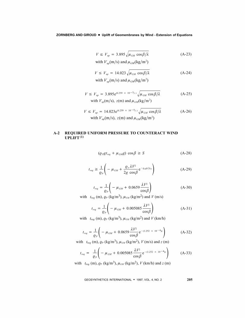
ZORNBERG AND GIROUD D Uplift of Geomembranes by Wind - Extension of Equations
205GEOSYNTHETICS INTERNATIONAL S 1997, VOL. 4, NO. 2
V ( Vup 3.895 $GM cos "#!)
V ( Vup 14.023 $GM cos "#!)
(A-23)
(A-24)
with Vup(m#s) and $GM(kg#m2)
with Vup(m#s) and $GM(kg#m2)
V ( Vup 3.895e(6.259 ! 10"5) z $GM cos "#!)
V ( Vup 14.023e(6.259 ! 10"5) z $GM cos "#!)
(A-25)
(A-26)
with Vup(m#s), z(m) and $GM(kg#m2)
with Vup(m#s), z(m) and $GM(kg#m2)
A-2 REQUIRED UNIFORM PRESSURE TO COUNTERACT WIND
UPLIFT(1)
(#Pgtreq$ $GMg) cos " ' S (A-28)
treq' 1
#P*" $GM$
#o !V2
2g cos "e"#ogz#po+ (A-29)
treq 1
#P*" $GM$ 0.0659
!V2
cos "+
with treq (m), #P (kg/m3), $GM (kg/m2) and V (m/s)
treq 1
#P*" $GM$ 0.005085
!V2
cos "+
with treq (m), #P (kg/m3), $GM (kg/m2) and V (km/h)
(A-30)
(A-31)
treq 1
#P*" $GM$ 0.0659
!V2
cos "e"(1.252 ! 10"4)z+
with treq (m), #P (kg/m3), $GM (kg/m2), V (m/s) and z (m)
treq 1
#P*" $GM$ 0.005085
!V2
cos "e"(1.252 ! 10"4)z+
with treq (m), #P (kg/m3), $GM (kg/m2), V (km/h) and z (m)
(A-32)
(A-33)

ZORNBERG AND GIROUD D Uplift of Geomembranes by Wind - Extension of Equations
206 GEOSYNTHETICS INTERNATIONAL S 1997, VOL. 4, NO. 2
A-3 EVALUATION OF EFFECTIVE SUCTION(1)
Se = S -- $GM g cos" (A-35)
Se !#(V2#2)" $GMg cos " (A-36)
Se !#o(V2#2)e"#o g z#po" $GMg cos " (A-37)
with Se(Pa), V(m#s) and $GM(kg#m2)
with Se(Pa), V(km#h) and $GM(kg#m2)
Se 0.6465!V2" 9.81$GM cos "
Se 0.050!V2" 9.81$GM cos "
(A-38)
(A-39)
Se 0.6465!V2e"(1.252 ! 10"4)z" 9.81$GM cos "
with Se(Pa), V(m#s), z(m) and $GM(kg#m2)
Se 0.050!V2e"(1.252 ! 10"4)z" 9.81$GM cos "
with Se(Pa), V(km#h), z(m) and $GM(kg#m2)
(A-40)
(A-41)
A-4 DETERMINATION OF GEOMEMBRANE TENSION AND STRAIN(2)
1$ w arc AB
L
2R'
2R sin '(A-45)
w '
sin '" 1 (A-46)
w 2TSeL
sin"1%SeL2T&" 1 (A-47)
with T T0$ Tw
w 12*2uL$ L2u+ sin"1,-.
22uL$ L2u
,/0" 1 (A-51)

ZORNBERG AND GIROUD D Uplift of Geomembranes by Wind - Extension of Equations
207GEOSYNTHETICS INTERNATIONAL S 1997, VOL. 4, NO. 2
SeL
2(T0$ J w) sin% SeL
2(T0$ J w)*1$ w+& (A-57a)
SeL
2J( 0$ w) sin% SeL
2J( 0$ w)*1$ w+& (A-57b)
Notes: (1)The revised equations incorporate the effect of slope inclination " through a term cos" that did not
exist in the original equations. Also, the notation treq is used, instead of Dreq in the original paper, to make it
clear that the dimension of the protective layer that is being calculated is the thickness (measured perpendicu-
larly to the slope), whereas the notationD is commonly used for the depth (measured vertically). For horizontal
slopes (" = 0) the revised equations are the same as those presented by Giroud et al. (1995).(2) The revised equations incorporate considerations discussed in Section 3.1 of this technical note regarding
the “uplift tension-strain” relationship, which relates the wind-induced strain component, w , to the total ten-
sion, T, in the geomembrane (T = T0 + Tw ). If the initial strain, 0 , and initial tension, T0 , in the geomembrane
are zero (i.e. if the total strain, ! w , and the total tension, T ! Tw), the revised equations are the same as those
presented by Giroud et al. (1995).

521GEOSYNTHETICS INTERNATIONAL S 1999, VOL. 6, NO. 6
Errata
UPLIFT OF GEOMEMBRANES BYWIND --EXTENSION OF EQUATIONS
TECHNICALNOTE FORERRATA: Zornberg, J.G. and Giroud, J.P., 1997, “Uplift
of Geomembranes by Wind – Extension of Equations”, Geosynthetics International,Vol. 4, No. 2, pp. 187-207.
PUBLICATION: Geosynthetics International is published by the Industrial FabricsAssociation International, 1801 County Road B West, Roseville, Minnesota
55113-4061, USA, Telephone: 1/651-222-2508, Telefax: 1/651-631-9334.Geosynthetics International is registered under ISSN 1072-6349.
REFERENCE FOR ERRATA: Zornberg, J.G. and Giroud, J.P., 1999, “Errata for‘Uplift of Geomembranes by Wind – Extension of Equations’”, Geosynthetics
International, Vol. 6, No. 6, pp. 521-522.
The authors inadvertently showed the wrong angle in Figure 2, p. 191 and used thewrong units in Equations A-18, A-20, A-24, and A-26, pp. 204-205, in their technicalnote, which appeared in Geosynthetics International, Vol. 4, No. 2.
ERRATUM FOR SECTION: 3.1 Uplift Tension-Strain Relationship
In Figure 2, p. 191 :
The angle at Point B (i.e. the angle between the geomembrane before uplift and the
geomembrane after uplift) should be instead of /2.
ERRATA FOR APPENDIX: A-1 GEOMEMBRANE SENSITIVITY TO
WIND UPLIFT
Equation A-18, p. 204, replace km/h with m/s to give :
!GM !GMreq! 0.0659"V2
cos #(A-18)
with !GMreq(kg m2) and V(m s)

ERRATA D Uplift of Geomembranes by Wind - Extension of Equations
522 GEOSYNTHETICS INTERNATIONAL S 1999, VOL. 6, NO. 6
Equation A-20, p. 204, replace km/h with m/s to give :
GM ! GMreq " 0.0659!V2
cos "e#(1.252 $ 10#4) z (A-20)
with GMreq(kg m2), V(m s) and z(m)
Equation A-24, p. 205, replace m/s with km/h to give :
V% Vup " 14.023 GM cos " !& (A-24)
with Vup(km h) and GM(kg m2)
Equation A-26, p. 205, replace m/s with km/h to give :
V% Vup " 14.023e(6.259 $ 10#5) z GM cos " !& (A-26)
with Vup(km h), z(m) and GM(kg m2)