Appendix F DA-10 Borrow Area Analysis - Mobile District 1: Time Series Plots ... (Chapter 4). To...
93
Appendix F DA-10 Borrow Area Analysis
Transcript of Appendix F DA-10 Borrow Area Analysis - Mobile District 1: Time Series Plots ... (Chapter 4). To...

Appendix F DA-10 Borrow Area Analysis

ERD
C/CH
L Le
tter
Rep
ort
MISSISSIPPI COASTAL IMPROVEMENT PROGRAM (MsCIP)
EFFECTS OF DA-10 REMOVAL ON CIRCULATION AND SEDIMENT TRANSPORT POTENTIAL WITHIN HORN ISLAND PASS AND LOWER
PASCAGOULA SOUND CHANNELS
Coa
stal
an
d H
ydra
ulic
s La
bor
ator
y
June 2012
Raymond S. Chapman, Alison S. Grzegorzewski, Phu V. Luong, Ernest R. Smith, S. Jarrell Smith and Michael W. Tubman
Approved for public release; distribution is unlimited.

ERDC/CHL Letter Report
ERDC/CHL Letter Report June 2012
MISSISSIPPI COASTAL IMPROVEMENT PROGRAM (MsCIP)
EFFECTS OF DA-10 REMOVAL ON CIRCULATION AND SEDIMENT TRANSPORT POTENTIAL WITHIN HORN ISLAND PASS AND LOWER
PASCAGOULA SOUND CHANNELS
Raymond S. Chapman, Alison S. Grzegorzewski, Phu V. Luong, Ernest R. Smith, S. Jarrell Smith and Michael W. Tubman
Coastal and Hydraulics Laboratory and Environmental U.S. Army Engineer Research and Development Center 3909 Halls Ferry Road Vicksburg, MS 39180

ERDC/CHL Letter Report
Abstract
ERDC-CHL was asked to perform wave, hydrodynamic and sediment transport potential modeling in support of the decision to remove or alter the existing dredged material placement site DA – 10 also known as Sand Island for use as a sand source for barrier island restoration. The effect of removing DA-10 was examined through preliminary numerical model analyses of waves, currents, and sediment transport potential. In addition, this preliminary analysis was designed to aid in the decision if more quantitative hydrodynamic and sediment transport analyses were required.
ERDC/CHL Letter Report
Contents
1 Introduction ........................................................................................................................... 5
2 Nearshore Wave Modeling ................................................................................................... 6
3 Circulation Modeling ........................................................................................................ 35
4 Sediment Modeling ........................................................................................................... 54
5 Summary ............................................................................................................................. 67
References ................................................................................................................................ 68
Appendix 1: Time Series Plots at Selected Locations With and Without DA-10 .................. 73

ERDC/CHL Letter Report
1 Introduction
The Mississippi mainland coast is bordered on the south by Mississippi Sound. Five barrier islands form the southern boundary of Mississippi Sound 10 to 15 miles to the south of the mainland. From west to east, the islands are Cat, Ship, Horn, Petit Bois, and Dauphin (Figure 1-1). All of Petit Bois, Horn, and Ship Islands and part of Cat Island are within the Gulf Islands National Seashore under the jurisdiction of the National Park Service (NPS). Tidal passes between the Gulf of Mexico and brackish waters of the Mississippi Sound consists of two deep draft Federal navigation channels located at Horn Island Pass and Ship Island Pass and two unmanaged inlets at Petit Bois Pass and Dog Keys Pass. To the west of Petit Bois Island and the Pascagoula Harbor Federal Navigation channel at Horn Island Pass lies the dredge material placement area DA-10, also known as Sand Island. DA-10 is being considered for use as a sand source in the MsCIP Comprehensive Plan to restore sediment to the Mississippi Barrier islands. Hurricane Katrina in 2005 severely impacted the mainland coast of Mississippi and the barrier island system. Although island breaching has been recorded historically along central Ship Island, the entrance between east and West Ship Islands has been continuous since 1969, when Hurricane Camille flooded all of coastal Mississippi. Camille Cut was significantly widened from approximately 2500 m to 5800 m by Hurricane Katrina in 2005. Within the scope of MsCIP, plans are being formulated to restore sediment to crucial areas of the barrier island system including Camille Cut at Ship Island
Figure 1-1. Mississippi barrier islands.

ERDC/CHL Letter Report
As part of this plan, a number of possible suitable sand sources have been identified. The dredged material placement site DA-10 is one of these sand sources. In order to address possible impacts of removing or altering DA-10, ERDC-CHL has undertaken a preliminary study to examine the effect of removing DA-10 through numerical model analyses of waves, currents, and sediment transport potential. It is important to note that due to the limited scope of work and schedule of this preliminary study, much of the hydrodynamic analysis utilized data of opportunity developed during earlier phases of the MsCIP and Bayou Casotte Harbor Channel Improvement Project. This preliminary analysis was designed to aid in the decision if more quantitative hydrodynamic and sediment transport analyses were required.
Chapter 2 documents the wave modeling approach required to provide radiation stress gradients for the hydrodynamics used to force the sediment transport potential model GTRAN. Chapter 1 provides an overview of the numerical wave model STWAVE and documents model validation in the Gulf of Mexico and within Mississippi Sound. Chapter 3 documents circulation modeling conducted to quantify the relative changes in circulation within Horn Island Pass and surrounding areas from alterations of DA-10. A combination of two-dimensional ADCIRC model and a three-dimensional numerical hydrodynamic model (CH3D-WES) was applied and provided hydrodynamic input to the sediment transport potential model GTRAN discussed in Chapters 4. Chapter 4 documents the sediment transport potential analysis. A summary of the findings is presented in Chapter 5.
2 Nearshore Wave Modeling
This chapter provides an overview of the nearshore numerical wave modeling approach and documents the wave model validation in the Gulf of Mexico and within the Mississippi Sound. Nearshore wave modeling was required to provide radiation stress gradients for the 3-D circulation model CH3D (Chapter 3). Wave modeling estimates were also required to provide input conditions for the sediment transport potential model GTRAN (Chapter 4). To assess nearshore wave model performance, a verification hindcast for the time period April-May 2010 was performed to coincide with a period of wave data collected by ERDC at two sites in the

ERDC/CHL Letter Report
vicinity of Ship Island. Chapter 2 in Wamsley et al. 2011 provides additional details regarding the 2010 field data collection effort.
STWAVE (Smith et al. 2001, Smith 2007) solves the steady-state wave action balance equation along piecewise, backward-traced wave rays on a Cartesian grid. STWAVE utilized 40 frequency bins, on the range 0.05-0.83 Hz and increasing in bandwidth linearly (Δf = 0.02), along with 72 directional bins of constant width 5 degrees. The parallel, full-plane version of STWAVE (henceforth referred to as STWAVE-FP) was applied at 200-m resolution in a nearshore domain that is 185 km x 170 km in spatial extent (Figure 2-1).
The STWAVE-FP nearshore wave modeling supported two main tasks during this project:
1) STWAVE-FP was used for the period April-June 2010 so that resulting radiation stress gradients could be implemented within the 3-D circulation model (Chapter 3). Radiation stress is the excess momentum flux carried by ocean waves. When waves break, momentum is transferred to the water column, forcing nearshore currents or changes in water level.
2) STWAVE-FP model was applied for the period April-June 2010 so that resulting wave parameters (height, period, direction) could be implemented with the sediment transport potential model to study the effects of the removal of Disposal Area 10 (DA-10) (Chapter 4).
STWAVE Grid Bathymetry/Topography
The STWAVE-FP grid bathymetry and topography were interpolated from the sl15v3 ADCIRC mesh. The circulation model ADCIRC covers a large domain including the entire Gulf of Mexico and the Atlantic Ocean eastward to the 60 degrees West longitude line. The high-resolution ADCIRC mesh includes over 2 million nodes and over 4 million elements, which the vast majority (over 50%) of the nodes and elements concentrated in the coastal Mississippi and Louisiana regions. The mesh bathymetry and topography were compiled from many sources, including: ETOPO1 in deep water (Amante and Eakins 2009), Coastal Relief DEMS (NOAA 2008), recent surveys by the Corps of Engineers and NOAA in the nearshore, as well as LIDAR surveys. Additional details on the ADCIRC sl15v3 mesh development and validation can be found in Bunya et al.

ERDC/CHL Letter Report
2010. For the existing post-Katrina condition, the ADCIRC mesh and STWAVE-FP grid were updated with additional detailed post-Katrina bathymetry derived from USGS data taken between June 2008 and June 2009 combined with EAARL LIDAR (Brock et al. 2007).
Figure 2-1. STWAVE-FP Existing Post-Katrina wave domain for March-June 2010 simulations.
In order to simulate the DA-10 removal scenario and resulting wave changes, the existing condition post-Katrina ADCIRC mesh was modified to include the DA-10 removal template that was provided to ERDC by the US Army Corps of Engineers Mobile District (SAM). The full-plane STWAVE domain was then created by direct interpolation from the modified ADCIRC mesh scenario.
Boundary Conditions
Wind Fields
The STWAVE-FP wind fields were spatially and temporally variable and interpolated from the ADCIRC modeling domain for the 2010 modeling simulation period. The April-June 2010 ADCIRC simulation used wind fields modeled by the Air Force Combat Climatology Center (AFCCC) on a 37×33 grid between 90.5778oW and 87.3240oW in longitude and

ERDC/CHL Letter Report
27.8353oN and 31.0099oN in latitude, with spatial resolution of 0.0986o in longitude and 0.0858o in latitude. The temporal resolution of the Air Force wind data are 1 hour. To assess the Air Force wind fields, the archived measured wind data from the NOAA NDBC Station #42040 was compared with the AFCCC data in 2010 (Figure 2-2). NDBC Station #42040 is located approximately 120 km south of Dauphin Island, AL (29°12'45" N 88°12'27" W) and the winds are measured 10-m above sea level. In addition, wind measurements from the NOAA National Ocean Service (NOS) Station at Gulfport Outer Range (GPOM6 #8744707) were also compared with the AFCCC wind data in 2010 (Figure 2-3). The Gulfport Outer Range Station is located north of West Ship Island in Mississippi Sound at 30°13’48” N 88°58’55” W and the winds are measured at 13.7 m above the site elevation. The station wind speed values were adjusted to 10-m wind speeds for comparison with the AFCCC wind data using the 1/7 exponential power law. The root-mean-square-error (RMSE) is 2.0 m/s at NDBC Station #42040 and the RMSE is 2.8 m/s at NOS Station at Gulfport Outer Range, i.e. the modeled AFCCC wind data show very good agreement with the measured wind data during the April-May 2010 period.
Figure 2-2. Comparison of Air Force wind speeds with measured NOAA NDBC Station #42040 wind speeds.

ERDC/CHL Letter Report
Figure 2-3. Comparison of Air Force wind speeds with measured NOAA NOS Gulfport Outer Range wind speeds.
Tides
Tidal water level adjustments were spatially and temporally variable within the STWAVE-FP model and were interpolated from the ADCIRC model output for the 2010 modeling simulation period. Seven tidal constituents were used during the ADCIRC simulations: K1, O1, Q1, M2, S2, N2, and K2.
Offshore Spectra
Directional wave spectra from the NOAA NDBC Station #42040 that is located approximately 120 km south of Dauphin Island, AL (29°12'45" N 88°12'27" W) were applied along the offshore boundary in STWAVE-FP. NDBC Station #42040 is located in a depth of approximately 165 m.
STWAVE-FP Validation
Field measurements are a critical asset for understanding wave processes and improving and validating nearshore wave models, such as STWAVE-FP. The validation of STWAVE-FP was performed with the ERDC-field data collected during March-July 2010 at Ship Island. In addition,
ERDC/CHL Letter Report
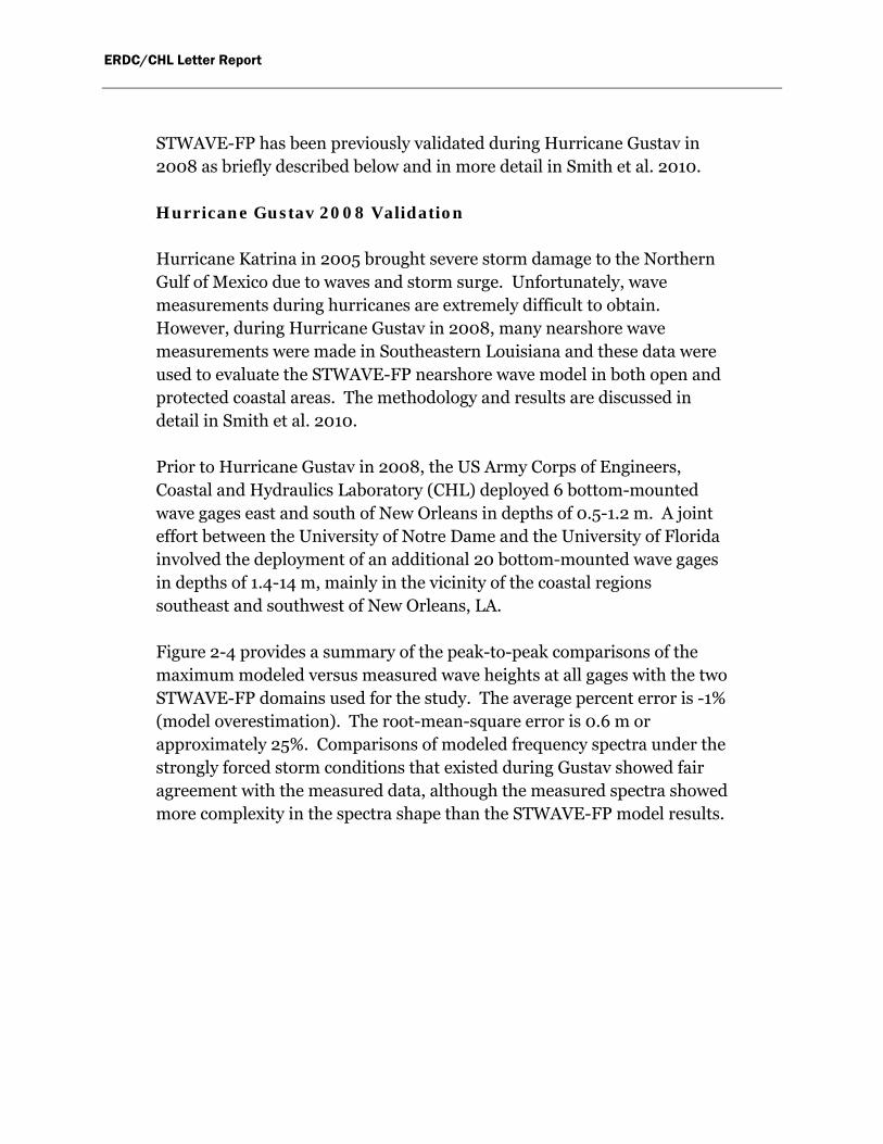
STWAVE-FP has been previously validated during Hurricane Gustav in 2008 as briefly described below and in more detail in Smith et al. 2010.
Hurricane Gustav 2008 Validation
Hurricane Katrina in 2005 brought severe storm damage to the Northern Gulf of Mexico due to waves and storm surge. Unfortunately, wave measurements during hurricanes are extremely difficult to obtain. However, during Hurricane Gustav in 2008, many nearshore wave measurements were made in Southeastern Louisiana and these data were used to evaluate the STWAVE-FP nearshore wave model in both open and protected coastal areas. The methodology and results are discussed in detail in Smith et al. 2010.
Prior to Hurricane Gustav in 2008, the US Army Corps of Engineers, Coastal and Hydraulics Laboratory (CHL) deployed 6 bottom-mounted wave gages east and south of New Orleans in depths of 0.5-1.2 m. A joint effort between the University of Notre Dame and the University of Florida involved the deployment of an additional 20 bottom-mounted wave gages in depths of 1.4-14 m, mainly in the vicinity of the coastal regions southeast and southwest of New Orleans, LA.
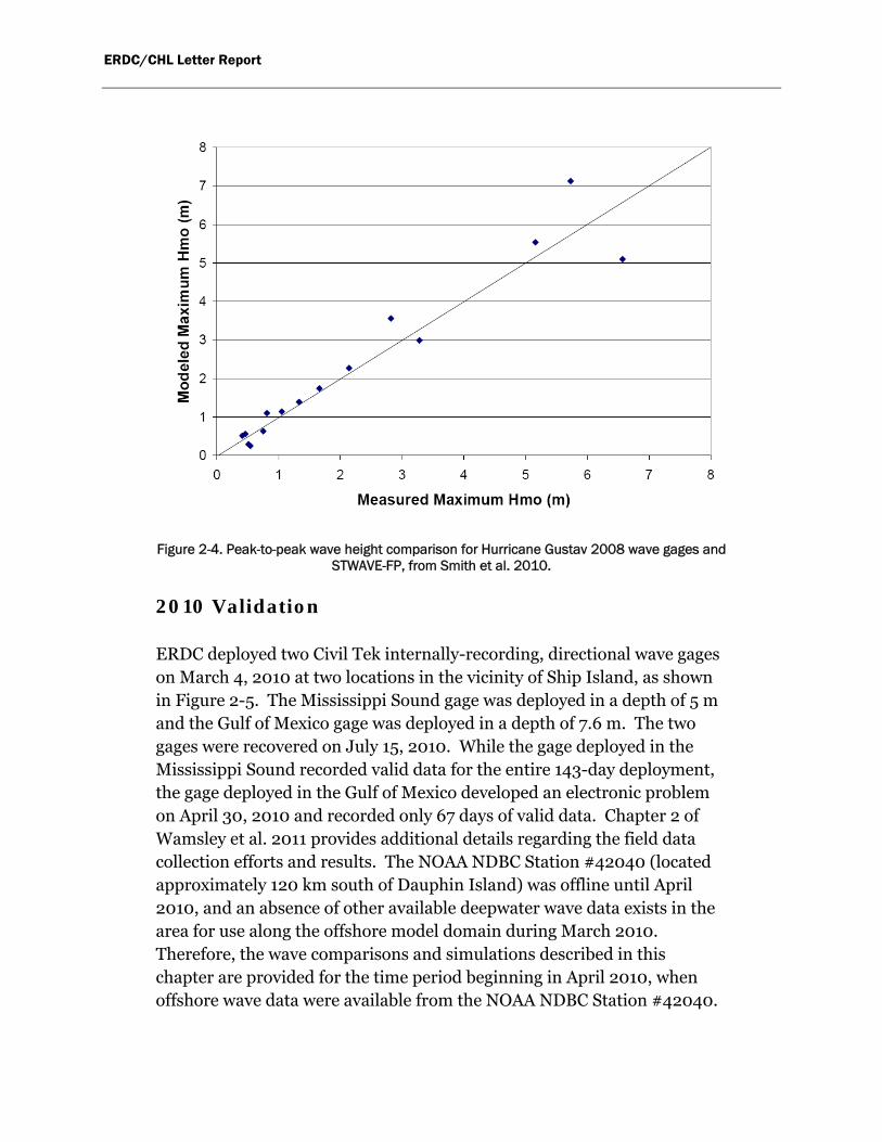
Figure 2-4 provides a summary of the peak-to-peak comparisons of the maximum modeled versus measured wave heights at all gages with the two STWAVE-FP domains used for the study. The average percent error is -1% (model overestimation). The root-mean-square error is 0.6 m or approximately 25%. Comparisons of modeled frequency spectra under the strongly forced storm conditions that existed during Gustav showed fair agreement with the measured data, although the measured spectra showed more complexity in the spectra shape than the STWAVE-FP model results.
ERDC/CHL Letter Report
Figure 2-4. Peak-to-peak wave height comparison for Hurricane Gustav 2008 wave gages and STWAVE-FP, from Smith et al. 2010.
2010 Validation
ERDC deployed two Civil Tek internally-recording, directional wave gages on March 4, 2010 at two locations in the vicinity of Ship Island, as shown in Figure 2-5. The Mississippi Sound gage was deployed in a depth of 5 m and the Gulf of Mexico gage was deployed in a depth of 7.6 m. The two gages were recovered on July 15, 2010. While the gage deployed in the Mississippi Sound recorded valid data for the entire 143-day deployment, the gage deployed in the Gulf of Mexico developed an electronic problem on April 30, 2010 and recorded only 67 days of valid data. Chapter 2 of Wamsley et al. 2011 provides additional details regarding the field data collection efforts and results. The NOAA NDBC Station #42040 (located approximately 120 km south of Dauphin Island) was offline until April 2010, and an absence of other available deepwater wave data exists in the area for use along the offshore model domain during March 2010. Therefore, the wave comparisons and simulations described in this chapter are provided for the time period beginning in April 2010, when offshore wave data were available from the NOAA NDBC Station #42040.

ERDC/CHL Letter Report
Figure 2-5. Location map showing the two 2010 ERDC wave gage deployment locations near Ship Island.
Direct Comparisons between Measured and Modeled Parameters
Figures 2-6 through 2-8 show the direct comparisons for the measured versus STWAVE-FP modeled zero-moment wave height, peak wave period, and wave direction at the Gulf of Mexico station. While a small over-prediction of wave height and under-prediction of peak wave period is observed, the STWAVE-FP model is able to reproduce these parameters within very good agreement. The comparison of modeled versus measured wave direction in Figure 2-8 shows excellent agreement between STWAVE-FP and the measurements, showing waves being predominantly propagated from the southeast at the Gulf of Mexico station.
Figures 2-9 through 2-11 show the direct comparisons for the measured versus STWAVE-FP modeled zero-moment wave height, peak wave period, and wave direction at the Mississippi Sound station. A more pronounced over-prediction pattern of wave height is observed at this station. In addition, an over-prediction of peak wave period is observed at this station. It is possible that bathymetrical inaccuracies account for some of the discrepancies observed between measurements and model predictions. Depth-limited and steepness-induced wave breaking processes are important in the numerical model simulations; therefore,

ERDC/CHL Letter Report
accurate bathymetry is critical. It may be more difficult to accurately measure wave heights less than 1 m, and that may account for some of the variability observed in Figure 2-9. Another explanation for the observed differences between measured versus modeled wave heights and periods is related to the pressure gages and the peak periods near or at the high-frequency cut-off for the spectral analysis. The high-frequency peaks in the spectra near the cut-off can be a result of amplification of noise due to large values of the pressure response function (applied to account for the depth attenuation of short-period wave components). Wave height in such situations may be either over-estimated (due to amplification of noise) or under-estimated (due to truncation of the energetic part of the spectrum). Wave periods would generally be under-estimated. In most applications, these truncated spectra would be disregarded for model verification, but for this application they provide valuable information about what was not measured. The direction comparison of measured versus modeled wave direction in Figure 2-11 shows excellent agreement between STWAVE-FP and the measurements, showing waves predominantly propagating from the southeast.
Figure 2-6. Measured vs. Modeled Hmo (m) at the Gulf of Mexico Station.

ERDC/CHL Letter Report
Figure 2-7. Measured vs. Modeled Tp (sec) at the Gulf of Mexico Station.
Figure 2-8. Measured vs. Modeled Dir (degrees clockwise from North) at the Gulf of Mexico
Station.

ERDC/CHL Letter Report
Figure 2-9. Measured vs. Modeled Hmo (m) at the Mississippi Sound Station.
Figure 2-10. Measured vs. Modeled Tp (sec) at the Mississippi Sound Station.

ERDC/CHL Letter Report
Figure 2-11. Measured vs. Modeled Dir (degrees clockwise from North) at the Mississippi Sound Station.
Wave Height Reduction Factor
A wave height reduction factor defined as the ratio of wave height at the Gulf of Mexico station to the wave height at the Mississippi Sound station was computed for the measured and modeled waves and is shown in Figure 2-12. The wave height reduction factor clearly demonstrates the attenuation in wave heights across Ship Island, from the exposed waves at the Gulf of Mexico station to the more sheltered waves at the Mississippi Sound station. While a small over-prediction of wave attenuation is shown in Figure 2-12 for the STWAVE-FP model when compared to the wave measurements, the wave model captured the reduction of waves across Ship Island with very good agreement overall. The average wave height reduction factor predicted by the model is 0.67, whereas the average wave height reduction factor observed in the measured data is 0.64.

ERDC/CHL Letter Report
Figure 2-12. Measured vs. Modeled Wave Reduction Factor demonstrating the attenuation of wave heights across Ship Island.
Time Series Figures at the Gulf of Mexico Station
Figures 2-13 through 2-15 show time series comparisons for the measured versus STWAVE-FP modeled zero-moment wave height, peak wave period, and wave direction at the Gulf of Mexico station. The STWAVE-FP model accurately captures the three largest increases in wave heights during the modeled time period that occurred on April 15, 24, and April 30, 2010. These are the only records in time when the wave gages recorded waves in excess of Hs = 1.5 m at the Gulf of Mexico Station. For these three wave events, the STWAVE-FP model is judged to show very good agreement with the measurements, with percent differences ranging from 4.3-5.7% as shown in Table 2-1.

ERDC/CHL Letter Report
Table 2-1: Wave Height Comparisons for three events at the Gulf of Mexico Station.
Date Hs (m)
Measured
Hs (m)
Modeled
% Difference; (Modeled-
Measured)/Measured
April 15, 2010 1.64 1.74 +5.7%
April 24, 2010 1.75 1.67 -4.6%
April 30, 2010 1.63 1.56 -4.3%
Figure 2-13. Time series of Measured and Modeled Hmo (m) at the Gulf of Mexico Station.

ERDC/CHL Letter Report
Figure 2-14. Time series of Measured and Modeled Tp (sec) at the Gulf of Mexico Station.
Figure 2-15. Time series of Measured and Modeled Direction (degrees clockwise from North) at the Gulf of Mexico Station.

ERDC/CHL Letter Report
Time Series Figures at the Mississippi Sound Station
Figures 2-16 through 2-18 show time series comparisons for the measured versus STWAVE-FP modeled zero-moment wave height, peak wave period, and wave direction at the Mississippi Sound station. A more pronounced pattern of over-prediction of wave height is observed at this station. In addition, an over-prediction of peak wave period is observed at this station. It is possible the bathymetrical inaccuracies account for some of the discrepancies between measurements and model predictions. Depth-limited and steepness-induced wave breaking processes are important in the numerical model simulations; therefore, accurate bathymetry is critical. The comparison of measured versus modeled wave direction in Figure 2-18 shows good agreement between STWAVE-FP wave and the measurements, showing waves being predominantly propagated from the south to southeast.
Figure 2-16. Time series of Measured and Modeled Hmo (m) at the Mississippi Sound Station.

ERDC/CHL Letter Report
Figure 2-17. Time series of Measured and Modeled Tp (sec) at the Mississippi Sound Station.
Figure 2-18. Time series of Measured and Modeled Direction (degrees clockwise from North)
at the Mississippi Sound Station.

ERDC/CHL Letter Report
Histograms for the Gulf of Mexico Station
Figures 2-19 through 2-24 show histograms for the measured and STWAVE-FP modeled zero-moment wave height, peak wave period, and wave direction at the Gulf of Mexico station. Both the measured (Figure 2-19) and the modeled (Figure 2-20) histograms for wave heights show that the vast majority of wave heights are Hmo < 1.0 m for the Gulf of Mexico station. While the measured waves (Figure 2-21) show the most frequently occurring peak periods as Tp = 3-4 sec, the modeled waves (Figure 2-22) show the most frequently occurring peak periods as Tp = 4-5 sec. Both the measured and modeled waves show excellent agreement for wave direction, with the predominant direction of wave propagation from the southeast, 135 degrees clockwise from North (Figures 2-23 and 2-24). Overall, STWAVE-FP is shown to model the measurements with very good agreement for the Gulf of Mexico station.
Figure 2-19. Histogram of the Measured Hmo (m) at the Gulf of Mexico Station.

ERDC/CHL Letter Report
Figure 2-20. Histogram of the Modeled Hmo (m) at the Gulf of Mexico Station.
Figure 2-21. Histogram of the Measured Tp (sec) at the Gulf of Mexico Station.

ERDC/CHL Letter Report
Figure 2-22. Histogram of the Modeled Tp (sec) at the Gulf of Mexico Station.
Figure 2-23. Histogram of the Measured Direction (clockwise from North) at the Gulf of Mexico Station.

ERDC/CHL Letter Report
Figure 2-24. Histogram of the Modeled Direction (clockwise from North) at the Gulf of Mexico Station.
Histograms for the Mississippi Sound Station
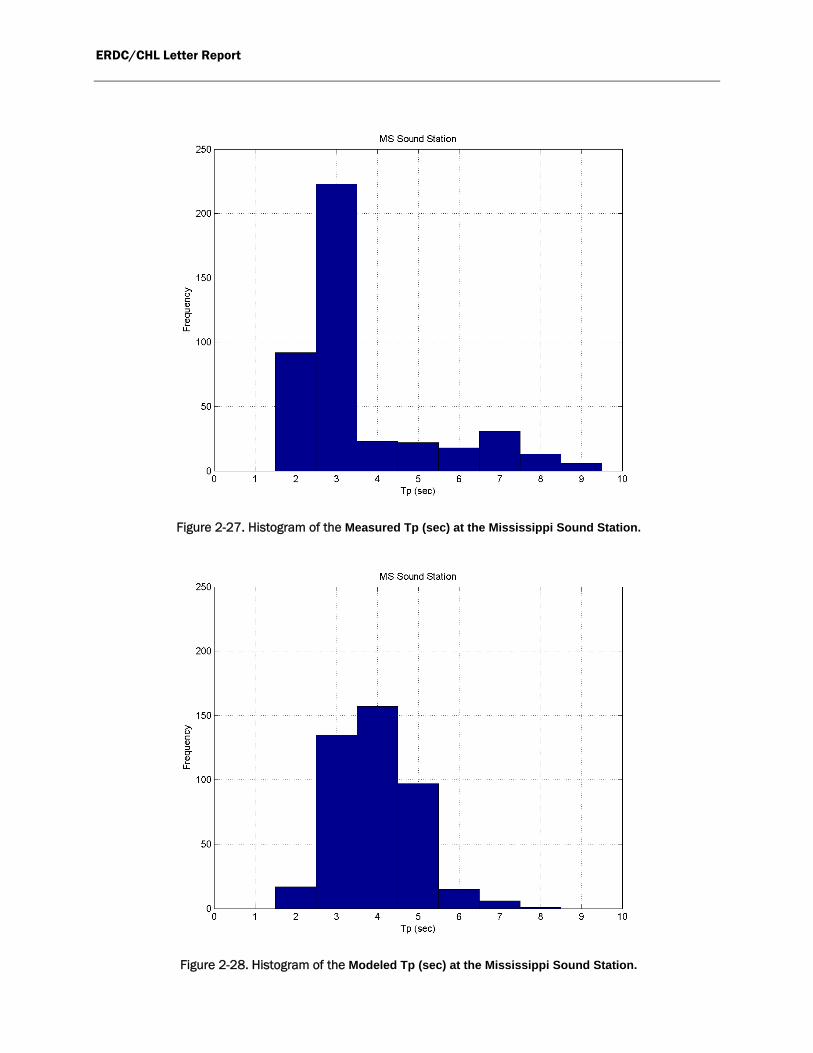
Figures 2-25 through 2-30 show histograms for the measured and STWAVE-FP modeled zero-moment wave height, peak wave period, and wave direction at the Mississippi Sound station. Both the measured (Figure 2-25) and the modeled (Figure 2-26) histograms for wave heights show that the vast majority of wave heights are Hmo < 0.6 m for the Mississippi Sound station. While the measured waves (Figure 2-27) show the most frequently occurring peak periods as Tp = 2-3 sec, the modeled waves (Figure 2-28) show the most frequently occurring peak periods as Tp = 3-5 sec. Both the measured and modeled waves show very good agreement for wave direction, with the predominant direction of waves propagating from the southeast to the south, i.e. 90-180 degrees clockwise from North (Figures 2-29 and 2-30). Overall, STWAVE-FP is shown to model the measurements with reasonable agreement at the Mississippi Sound station.

ERDC/CHL Letter Report
Figure 2-25. Histogram of the Measured Hmo (m) at the Mississippi Sound Station.
Figure 2-26. Histogram of the Modeled Hmo (m) at the Mississippi Sound Station.
ERDC/CHL Letter Report
Figure 2-27. Histogram of the Measured Tp (sec) at the Mississippi Sound Station.
Figure 2-28. Histogram of the Modeled Tp (sec) at the Mississippi Sound Station.

ERDC/CHL Letter Report
Figure 2-29. Histogram of the Measured Direction (degrees clockwise from North) at the Mississippi Sound Station.
Figure 2-30. Histogram of the Modeled Direction (degrees clockwise from North) at the Mississippi Sound Station.

ERDC/CHL Letter Report
Additional Measures of Model Performance
To quantify the predictive capability of STWAVE-FP, the root-mean-square-error (RMSE) was computed at the Gulf of Mexico and Mississippi Sound stations. The RMSE of the wave height is 0.27 m at the Gulf of Mexico station and 0.23 m at the Mississippi Sound station. To quantify the performance of ocean wave models, a scatter index (SI) is sometimes used (Zambreski, 1989, 1991; Komen et al., 1994; Romeiser, 1993), which is defined as the RMSE normalized with the mean observed value. The SI for the wave height is 0.45 at the Gulf of Mexico station and 0.76 at the Mississippi Sound station.
As discussed by Ris et al. (1999), this scatter index may appear to understate the skill of the wave model, as it tends to be large in some coastal applications. The reason is that the RMSE of the wave height is normalized with the mean observed wave height, which is usually rather small in coastal regions (0.6 m and 0.3 m at the Gulf of Mexico station and Mississippi Sound station, respectively). Therefore, the SI attains high values of 0.45 and 0.76 at the Gulf of Mexico station and Mississippi Sound station, respectively, due to being normalized by the small mean observed waves.
Ris et al. (1999) proposed two alternative model performance indices to supplement the standard RSME and SI calculations, referred to as the model performance index (MPI) and the operational performance index (OPI).
The model performance index (MPI) is considered to better diagnose the modeling performance and indicates the degree to which the model reproduces the observed changes of the waves, where MPI is defined as 1 minus the RMSE normalized with the root-mean-square (RMS) of the observed changes. The definition of RMS of the observed changes is identical to that of RMSE, except that all computed values are replaced by the observed incident values. For a perfect model, RMSE = 0 and the value of the MPI = 1, whereas MPI = 0 for a model that (erroneously) predicts no changes (RMSE = RMS of the observed changes). The MPI for the wave height is 0.58 at the Gulf of Mexico station and 0.74 at the Mississippi Sound station.
The more predictive operational performance index is defined as the RMSE normalized with the incident observed values. It is predictive and

ERDC/CHL Letter Report
operational in the sense that for a given value of the OPI (presumably a characteristic of the model and its implementation for a particular region), an error estimate can be made on the basis of incident wave conditions, prior to the computations. The OPI for the wave height is 0.23 at the Gulf of Mexico station and 0.22 at the Mississippi Sound station.
To determine the systematic part of the model performance, the bias is also considered. The bias is simply the mean error, defined as the STWAVE-FP model results minus the observations. The bias for the wave height is 0.16 m at the Gulf of Mexico station and 0.16 m at the Mississippi Sound station.
To quantify the predictive capability of STWAVE-FP, measures of model performance such as root-mean-square-error, scatter index, model performance index, operational performance index, and bias were computed for wave height at the Gulf of Mexico station at and the Mississippi Sound station and a summary of results are provided in Table 2-2.
Table 2-2: Performance of STWAVE-FP for Wave Height
Measure of
Performance
Gulf of
Mexico
Station
Mississippi
Sound
Station
Root-mean-square-error,
RMSE 0.27 m 0.23 m
Scatter index, SI 0.45 0.76
Model performance index,
MPI 0.58 0.74
Operational performance
index, OPI 0.23 0.22
Bias 0.16 m 0.16 m

ERDC/CHL Letter Report
In summary, the STWAVE-FP model compared with very good agreement to the measurements, overall. The wave model also predicted the attenuation in wave heights across Ship Island rather well, from the exposed waves at the Gulf of Mexico station to the more sheltered waves at the Mississippi Sound station. The average wave height reduction factor predicted by the model is 0.67, whereas the average wave height reduction factor observed in the measured data is 0.64, where the wave height reduction factor is defined as the ratio of wave height at the Gulf of Mexico station to the wave height at the Mississippi Sound station.
Summary and Wave Sensitivity to DA-10 Removal This section provides an overview of the nearshore numerical wave modeling approach and documentes the wave model validation in the Gulf of Mexico and within Mississippi Sound. STWAVE-FP nearshore wave modeling supported two main tasks during this project: STWAVE-FP model was applied for the period April-June 2010 so that the resulting radiation stress gradients could be applied within the 3-D circulation model (Chapter 3). In addition, STWAVE-FP results were used to provide input conditions for the sediment transport potential model GTRAN (Chapter 4).
Three representative locations were studied in order to determine the localized wave effects due to the removal of DA-10 (Figure 2-31). The time series of wave heights for the Existing and DA-10 Removal scenarios are shown in Figures 2-32 through 2-34 for each of the three locations. The maximum wave height during the simulated time period is approximated 1 m and the time-averaged mean wave height is approximately 0.5 m for the Existing conditions at three locations studied.

ERDC/CHL Letter Report
Figure 2-31. Location map showing GTRAN calculation points (red) and three detailed
locations for wave sensitivity analysis (black outline).
As expected, all three locations experienced an increase in wave energy due to the removal of DA-10. Under the Existing conditions, waves are physically obstructed by DA-10 and less wave energy is allowed to propagate into the Mississippi Sound. However, under the DA-10 Removal scenario, increased wave heights can be attributed to additional wave energy that is no longer dissipated by the material at DA-10 and these waves continue to propagate shoreward in its lee. The time-averaged wave height amplification is approximately 0.2 m for the 3 representative locations studied. The largest wave height increases are observed at and immediately leeward of DA-10, which was removed (degraded) to a subaqueous shoal for the DA-10 Removal scenario.

ERDC/CHL Letter Report
Figure 2-32. Time series of Hs (m) at Location #1 (Figure 2-31) for Existing and DA-10 Removal Scenarios.
Figure 2-33. Time series of Hs (m) at Location #2 (Figure 2-31) for Existing and DA-10
Removal Scenarios.

ERDC/CHL Letter Report
Figure 2-34. Time series of Hs (m) at Location #3 (Figure 2-31) for Existing and DA-10
Removal Scenarios.
3 Circulation Modeling
ADCIRC Grid, Model Forcing and Calibration
An existing pre-Katrina calibrated ADCIRC model was updated to represent post-Katrina Mississippi Sound (Figure 3-1). Post-Katrina bathymetry in Mississippi Sound and along the Chandeleur Islands is based on 2008 – 2009 surveys conducted by the United States Geological Survey (USGS) (Buster and Morton, 2011) and the US Army Corps of Engineers, Mobile District.

ERDC/CHL Letter Report
Figure 3-1. ADCIRC grid.
ADCIRC forcing consisted of wind and tidal constituent inputs. Tidal forcing was applied to the grid by imposing tidal water-level variations along its open-ocean boundary. Seven tidal constituents (i.e., K1, O1, Q1, M2, S2, N2 and K2) from the East Coast 2001 Data Base of Tidal Constituents (Mukai et. el., 2002, CHL Technical Note CHETIN-IV-40) were used in the simulations. Hourly wind speeds and directions for pre-Katrina simulations were available from NOAA National Data Buoy Center (NDBC) Stations DPIA1 on the eastern end of Dauphin Island and B42007 located 41 km south-southeast of Biloxi (30o 5.4’ N, 88o 46.14’ W). For the post-Katrina July 14 to 20, 2009 period, wind data were available from the U. S. Air Force Weather Agency Meteorological Office prediction model (https://afweather.afwa.af.mil/weather/met/met_home.html).
Bottom ADCP current velocity and water surface elevation measurements from a gage deployed north of Petit Bois Island (30.13 N , 88 30.27 W) were used for model data comparisons during the July 14 to 20, 2009 time period. This gage was deployed near the navigation channel through Horn Island Pass (HIP, Figure 1-1) in support of the Bayou Casotte Channel improvement Project. The data were processed to provide water

ERDC/CHL Letter Report
surface levels and depth-averaged current estimates. A comparison of ADCIRC simulated and measured current and elevation estimates are shown in Figure 3-2. The water surface elevation and depth-averaged current comparisons show reasonably good agreement in both phase and amplitude. It is known that meteorological forcing plays a significant role in the hydrodynamic response of Mississippi Sound. Consequently, it is important to note that when assessing the quality of the model data comparisons, it must be kept in mind that the meteorological forcing data used were input files of opportunity and not a project specific and analyzed climatology (IPET (2007) and Cox, A.T. and V.J. Cardone (2007)). In addition, atmospheric pressure forcing was not applied in these simulations.
Figure 3-2. ADCIRC stimulated (red lines) and measured (black lines) currents and water elevations at HIP for the July 14 to 20, 2009 ADCIRC calibration simulation.

ERDC/CHL Letter Report
In support of the CH3D circulation and GTRAN sediment transport potential modeling efforts, ADCIRC simulations with and without DA-10 (Figure 3-3) were preformed for the period March 2 to June 14, 2010, which generated tidal boundaries for CH3D. Upon removal of DA-10 from the grid, a depth of 2.4 m below mean tide level was specified.
Using ADCIRC simulation results generated in support of the Ship Simulator Task within the Bayou Casotte Channel Widening, an analysis of change in current structure within the HIP and Lower Pascagoula Channel was undertaken. Simulations were performed to examine peak flood and ebb conditions on May 1, 2010 with winds of 25 knots blowing steadily from the west (270o) and from the south-southeast (157.5o) with and without DA-10 in place. Figures 3-4 and 3-5 present the current structure for the west winds at a period of maximum flood and maximum ebb with and without DA-10, respectively. Figures 3-6 and 3-7 show maximum flood and ebb with the south-southeast winds.
Figure 3-3. ADCIRC grids, Horn Island Pass for the existing condition and without DA-10.

ERDC/CHL Letter Report
Figure 3-4. ADCIRC simulated currents at maximum flood for the existing condition and without DA10 with west winds of 25 knots.
Figure 3-5. ADCIRC simulated currents at maximum ebb for the existing condition and without DA10 with west winds of 25 knots.

ERDC/CHL Letter Report
Figure 3-6 . ADCIRC simulated currents at maximum flood for the existing condition and without DA10 with south-southeast winds of 25 knots.
Figure 3-7. ADCIRC simulated currents at maximum ebb for the existing condition and without DA10 with south-southeast winds of 25 knots.
Figures 3-8 and 3-9 present difference plots of current speed anddirection for the west wind simulation at maximum flood and ebb. The difference values in the figures are computed by subtracting the existing currents from the without DA-10 currents.

ERDC/CHL Letter Report
Figure 3-8. ADCIRC simulated current speed and direction differences at maximum flood between the existing condition and without DA10
with west winds of 25 knots
Figure 3-9. ADCIRC simulated current speed and direction differences at maximum ebb between the existing condition and without DA10 with west winds of 25 knots
Figures 3-10 and 3-11 present difference plots of current speed and direction for the south-southeast wind simulation at maximum flood and ebb, respectively.

ERDC/CHL Letter Report
Figure 3-10. ADCIRC simulated current speed and direction differences at maximum flood between the existing condition and without DA10 with south-southeast winds of 25 knots.
Figure 3-11. ADCIRC simulated current speed and direction differences at maximum ebb between the existing condition and without DA10 with south-southeast winds of 25 knots.
Time series plots of 60-hr simulations were generated to show differences in the currents for the existing condition and with DA10 reduced, at 11 locations starting about one mile south of Horn Island Pass in the Gulf, going along the center of the navigation channel through the Pass, and ending about one mile north of the Pass in the Sound. The locations of the comparison points are shown in Figure 3-12. The time series plots similar

ERDC/CHL Letter Report
to Figures 3-13 and 3-14 may be found in Appendix 1, where the figure numbering of 3-15 through 3-24 is retain.
For the two wind conditions simulated (west winds and winds from the south-southeast), it was observed that for west winds during flood, current speeds in the channel through the Pass are lower (maximum decrease: -0.15 m/s), while currents speeds in the channel north of the Pass are higher (maximum increase: 0.37 m/s). South of the Pass there is very little difference in the channel (a smaller than -0.02 m/s decrease). For west winds during ebb, there are lower current speeds north of and in the Pass (maximum decrease: -0.09 m/s), and higher current speeds south of the Pass (maximum increase: 0.18 m/s). For winds from the south-southeast during flood, current speeds are lower in and north of the Pass (maximum decrease: -0.17 m/s) and higher south of the Pass (maximum increase: 0.09 m/s). During ebb and south-southeast winds, there are lower current speeds in the Pass (maximum decrease: -0.08 m/s) and higher speeds north (maximum increase: 0.39 m/s) and south (maximum increase: 0.18 m/s) of the Pass. In each case, the differences are less that 1%.
Figure 3-12. Locations of time-series comparison plots.

ERDC/CHL Letter Report
Figure 3-13. Simulated current speeds and directions for the existing condition (black) and without DA10 (red) for locations one (top) and two (bottom)
with west winds of 25 knots.

ERDC/CHL Letter Report
Figure 3-14. ADCIRC simulated current speed and direction differences (existing minus without DA-10) of currents plotted in Figure 3-13.
CH3D Grid, Model Forcing and Calibration
The Curvilinear Hydrodynamic 3-D (CH3D-WES) model is routinely applied in 3-D hydrodynamic and water quality modeling studies at the Engineering Research and Development Center (ERDC), Mississippi. Within the scope of MsCIP, an updated version of CH3D was developed and calibrated. The single-block Mississippi Sound grid is 450x364 with 5 vertical sigma layers. This Mississippi Sound grid extends from Lake Pontchartrain, LA to Mobile Bay, AL. The single-block grid was then decomposed into 5-block grid for this study (Figure 3-37). Again, as previously explained, much of the differences seen in the model data

ERDC/CHL Letter Report
comparisons can be attributed to the lack of site specific wind and atmospheric pressure forcing.
Figure 3-37. Mississippi Sound CH3D 5-block Grid.
The initial calibration was in support of a MsCIP Water Quality Study, in which simulations were performed for March – September 1998. A tidal prism and storm event calibration was performed comparing ADCIRC, CH3D, and NOAA predicted water surface elevations at Dauphin Island Alabama (Figures 3-38) and observed water surface elevations at Waveland Mississippi (Figures 3-39). It is seen in these figures that the water surface elevation is tracked well at both locations, where the phase consistency is shown in Figure 3-38, and the response to storm wind forcing is shown in Figures 3-39.

ERDC/CHL Letter Report
Figure 3-38. Comparison of predicted water surface level with ADCIRC and CH3D predictions at Dauphin Island, AL.
Figure 3-39. Comparison of Observed water surface level with ADCIRC and CH3D predictions at Waveland, MS.
The CH3D grid and bathymetry then were updated to a post-Katrina surface using the 2008 - 2009 USGS bathymetric survey (Buster and Morton, 2011) data provided by the District. Validation simulations were
ERDC/CHL Letter Report
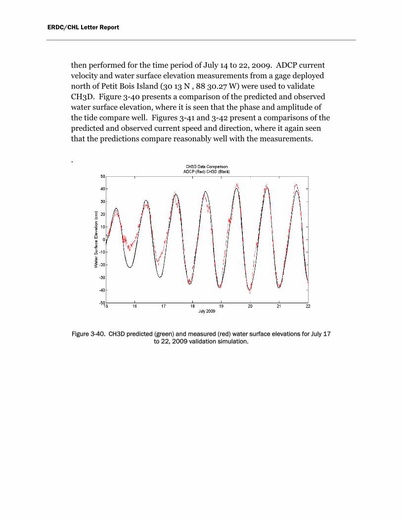
then performed for the time period of July 14 to 22, 2009. ADCP current velocity and water surface elevation measurements from a gage deployed north of Petit Bois Island (30 13 N , 88 30.27 W) were used to validate CH3D. Figure 3-40 presents a comparison of the predicted and observed water surface elevation, where it is seen that the phase and amplitude of the tide compare well. Figures 3-41 and 3-42 present a comparisons of the predicted and observed current speed and direction, where it again seen that the predictions compare reasonably well with the measurements.
.
Figure 3-40. CH3D predicted (green) and measured (red) water surface elevations for July 17 to 22, 2009 validation simulation.

ERDC/CHL Letter Report
Figure 3-41. CH3D predicted (green) and measured (red) current speed for July 17 to 22,
2009 validation simulation.
Figure 3-42. CH3D predicted (green) and measured (red) current speed for July 17 to 22, 2009 validation simulation.
CH3D grid depths in the vicinity of DA-10 were updated according to the NOAA chart 11357 and the 2008 - 2009 USGS bathymetric survey data (Buster and Morton, 2011) provided by the District. DA-10 was replaced

ERDC/CHL Letter Report
on the grid with depths 2.4 m below mean tide level. CH3D multi-block grid model was then setup for simulations on the existing DA10 grid as well as the reduced DA-10 grid. The Horn Island Pass block is shown in Figure 3-43 with DA-10, and on Figure 3-44 without DA-10.
Simulations during the time period of March 2 to June 14, 2010 were performed to supply near bottom velocities in support of GTRAN. An analysis of near bottom current structure in the vicinity of Horn Island Pass was next undertaken. Near bottom currents generated during a CH3D simulation correspond to the bottom layer of a five level sigma grid and consequently the vertical position of the near bottom velocity is relative to the depth. Specifically, a computation cell with a 10 m depth has a near bottom velocity that is 1 m above the seafloor.
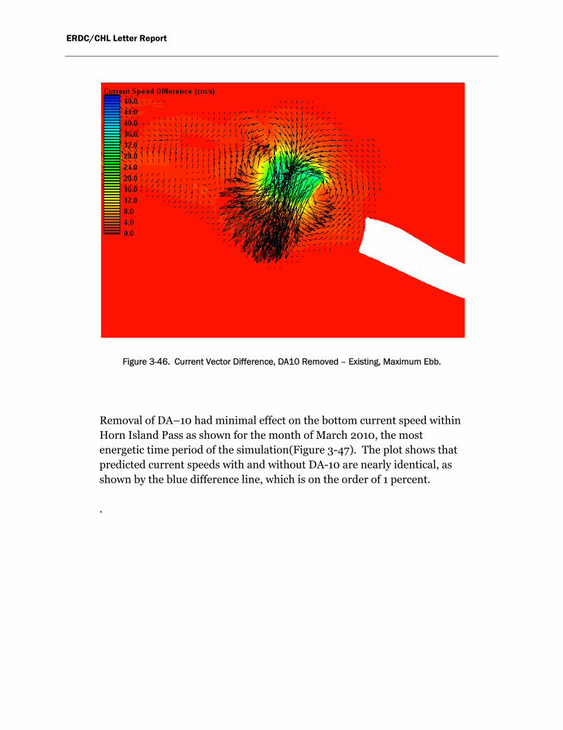
Simulations with and without DA-10 were performed and the differences in predicted near bottom current components were computed. Figures 3-45 and 3-46 present contour and vector plots of velocity vector differences at maximum flood and ebb, respectively, in which it is seen that the magnitude of appreciable velocity change is restricted to the DA-10 footprint.
Figure 3-43. DA10 Existing Grid.

ERDC/CHL Letter Report
Figure 3-44. DA10 Removed Grid.
Figure 3-45. Current Vector Difference, DA10 Removed – Existing, Maximum Flood.
ERDC/CHL Letter Report
Figure 3-46. Current Vector Difference, DA10 Removed – Existing, Maximum Ebb.
Removal of DA–10 had minimal effect on the bottom current speed within Horn Island Pass as shown for the month of March 2010, the most energetic time period of the simulation(Figure 3-47). The plot shows that predicted current speeds with and without DA-10 are nearly identical, as shown by the blue difference line, which is on the order of 1 percent.
.

ERDC/CHL Letter Report
Figure 3-47. Comparison of HIP Channel Current Speeds, Existing and DA10 Removed
Similarly, alteration of current direction within Horn Island Pass channel is small (Figure 3-48). Specifically, the change in current with and without the presence of DA-10 appears to be related to change in phase of the tide.
Figure 3-48. Comparison of HIP Channel Current Direction, Existing – DA-10 Removed

ERDC/CHL Letter Report
4 Sediment Transport
A primary focus of this study was to identify possible changes in sedimentation in the Pascagoula channel associated with removal of dredged material from DA 10. To address this concern, the numerical sediment transport model GTRAN was applied to the study area. GTRAN is utilized to estimate sand transport magnitudes and pathways in the area of DA-10 with DA-10 in place and with it removed to a 2.4-m depth (MTL).
This chapter provides background of the GTRAN model, input parameters for DA-10, and results from the model application.
GTRAN Model Description
To estimate sediment transport, predictive techniques were applied with available knowledge of environmental conditions and sediment properties. The sediment transport model GTRAN applied near-bottom currents calculated by CH3D and waves estimated by STWAVE to predict transport magnitudes and pathways in the study area. GTRAN is a local sediment transport model, which estimates potential transport rate (assuming unlimited sediment supply) and does not solve for continuity of mass or bed change. GTRAN includes effects of waves and currents on transport of non-cohesive sediment.
Transport Methods
GTRAN calculates sediment transport through a collection of sediment transport methods, algorithms that estimate sediment movement under specific wave and current conditions. Presently there are no sediment transport methods that are universally applicable to all environments and sediment types. For instance, a transport method developed for cobbles and boulders in an alpine stream is not likely to correctly represent sediment transport in an estuary or open-coast application. To correctly and reliably estimate sediment transport, the transport method must represent first-order transport processes within the region of application. A general description and overview will be given for each transport method applied.
Wikramanayake and Madsen Transport Method
Under contract with the U.S. Army Corps of Engineers, Dredging Research Program (DRP), researchers at Massachusetts Institute of Technology
ERDC/CHL Letter Report
developed non-cohesive sediment transport algorithms for combined wave-current environments. The algorithms include the effects of varia-tion between current and wave directions. The methods are outlined in DRP reports (Madsen and Wikramanayake 1991; Wikramanayake and Madsen 1994a) and were specifically designed for nearshore transport in high-energy regions, although the initial validation and calibration were performed outside the surf zone. User input includes near-bottom orbital velocity, mean currents, bed slope, and grain size.
The method uses a time-invariant turbulent eddy viscosity model and a time-varying near-bottom concentration model to estimate suspended sediment transport fluxes. The method first calculates the bed roughness, using methods outlined by Wikramanayake and Madsen (1994b). Bed load and suspended sediment concentrations are then calculated using bottom shear stress. Estimates of vertical variation in suspended sediment con-centration are based on a non-dimensional, time-varying, near-bottom reference concentration, Cr(t). This concentration can be estimated as:
*
b o cr
rcr
C tC t
(4-1)
where:
Cb = volume fraction of sediment in the bed γo = empirical resuspension coefficient Ψ*(t) = the Shield’s parameter based on instantaneous, skin-friction shear
stress Ψcr = the critical Shield’s parameter
Laboratory experiments have demonstrated that γo decreases with increasing Shield’s parameter or wave skin friction shear stress. However, data were insufficient to develop empirical methods to relate the resuspension coefficient to Shield’s parameter and constant values of γo are applied for rippled and flat beds, respectively. The Shield’s parameters are defined by:
**
501
u tt
s gd
(4-2)

ERDC/CHL Letter Report
1 tancr (4-3)
where:
u* (t) = bed shear velocity s = specific gravity of sediment g = acceleration due to gravity d50 = median grain diameter α1 = coefficient dependent on the local Reynolds number φ = angle of repose of the sediment grains The reference concentration is used to estimate vertically varying concen-trations in the water column due to steady and oscillatory currents. The estimated suspended sediment concentration is coupled with the vertically varying velocities to estimate the total suspended sediment flux.
The Wikramanayake and Madsen model also includes a method for esti-mating instantaneous bed-load flux based on the Meyer-Peter and Müller (1948) formula. This instantaneous bed-load flux, Qb , is estimated by:
* '50 50
'
81
cos21 tan
tan
cr bb
t sw bL
f
td s gd tQ t
t
(4-4)
where βL= h/6δ, h is the water depth, δ is the boundary layer length scale, Φt is the angle between the current and the wave direction, Φsw is the angle between the wave direction and bottom slope, and τb’ (t) is the instantaneous skin friction shear stress.
Wikramanayake and Madsen (1994a) performed several tests to compare their results to field measurements in wave/current environments and found that the model accurately predicted the current-related and wave-related sediment fluxes and distributions in the water column. No verifi-cation was performed for the bed-load model estimates. Field verification of the transport method has been performed by CHL against data sets from the Columbia River mouth (Gailani et al. 2003) and in the surf zone at the Field Research Facility, Duck, North Carolina. For both field verification exercises, the Wikramanayake and Madsen transport method agreed well with the data when wave-current shear stresses were strong
ERDC/CHL Letter Report
enough that suspended load transport dominates but overestimated sediment transport rates under less energetic conditions. Therefore other methods of approximating sediment transport were applied under bedload-dominated or current-dominated transport conditions.
Soulsby Bedload Transport Method
Soulsby (1997) developed a formula for combined wave-current bedload by integrating the current-only bedload formula of Nielsen (1992) over a single sinusoidal wave cycle. The formula is expressed as follows:
1
21 12x m m cr (4-5a)
1
22 12 0.95 0.19cos 2x w m (4-5b)
x1 x2maximum of and x (4-5c)
1
3 2501bx xq g s d (4-5d)
subject to Φx = 0 if θcr ≥ θmax
where:
θm = mean Shield’s parameter over a wave cycle θcr = critical Shield’s parameter for initiation of motion φ = angle between current direction and direction of wave travel θw = amplitude of oscillatory component of θ due to waves qbx = mean volumetric bedload transport rate per unit width θmax= maximum Shield’s parameter from combined wave-current stresses Soulsby’s combined wave-current bedload transport method was applied when sediment suspension was estimated to be near zero.
Van Rijn Current-dominated Transport Method
The Van Rijn (1984) current-only total transport method was parame-terized by Soulsby (1997) from Van Rijn’s comprehensive theory of sediment transport in rivers. Although the method was developed for sediment transport in the riverine environment, the method may also be appropriately applied in the marine environment under conditions for which waves contribute little to the bottom shear stress. The simpler,

ERDC/CHL Letter Report
parameterized formulae presented here approximate the full theory within ±25 percent and were developed for water depths between 1 and 20 m, velocities between 0.5 and 5 m/s, d50 between 0.1 and 2 mm, and for fresh water at 15 deg C. The resulting parameterized method estimates transport by the following simpler formulation:
t b sq q q (4-6)
2.41.2
501
250
0.0051
crb
U U dq Uh
hs gd
(4-7)
2.4
0.650*1
250
0.0121
crs
U U dq Uh D
hs gd
(4-8)
where:
0.1
50 10 5090
0.6
50 10 5090
40.19 log for 0.1 0.5
48.50 log for 0.5 2.0
cr
cr
hU d d mm
d
hU d d mm
d
1
3
* 502
1g sD d
qb=bedload transport qs=suspended load transport U = depth-averaged current h = water depth d90 = sediment diameter for which 90 percent is finer by weight
Model Setup
GTRAN requires X, Y, and Z coordinates for each location where sediment transport is to be calculated. The computational domain of the model for DA-10 was defined by 540 discrete points variably spaced between 80 and 740 m in the vicinity of Horn Island Pass. The number of points and spacing were selected so that there were sufficient points to define transport within Pascagoula Channel, and adjacent areas of interest with

ERDC/CHL Letter Report
the primary emphasis on capturing the area at and around DA-10 (Figure 4-1).
GTRAN input includes bed grain size, bathymetry, and hydrodynamic/environmental conditions. Sediment size distributions were assumed uniform within the domain. Input grain size was based on sample S-1-09 taken at DA10 with d50 = 0.32 mm, d90=0.41 mm and d10 = 0.25 mm.
With the initial bed conditions specified, the model applies environmental forcing conditions from STWAVE model and CH3D hydrodynamic model results at each of the computational points. The temporal resolution of the wave and current information is 1 hr. With local conditions determined, the model proceeds to estimate the wave/current-related bottom shear stresses and to estimate the depth of the active sediment layer. The
Figure 4-1. GTRAN calculation points. Contours indicate bathymetry in meters relative to Mean Sea Level.

ERDC/CHL Letter Report
transport method for each position and time step is selected based upon the relative contributions of waves and near-bed currents on the bed stress and whether the transport regime is bedload dominated or influenced by suspended sediment transport. Transport magnitude is computed by the appropriate transport regime discussed above and stored for each location and time interval.
Results
Three-month simulations from March 2 to June 14, 2010 were performed for the existing condition and with DA-10 removed. Figures 4-2 and 4-3, present the sand transport rate, averaged over the duration of each simulation. For the existing condition (Figure 4-2), the greatest sand transport rates occur at the shallow shoals exposed to the open gulf waves.
Figure 4-2. Estimated average sand transport rate for existing configuration. Contours indicate bathymetry in meters relative to Mean Sea Level.

ERDC/CHL Letter Report
Average transport rates are zero or near zero at DA-10, and are very low in the lee (north) of DA-10 due to wave sheltering. The sediment transport patterns with DA-10 removed (Figure 4-3) are generally similar, with two notable exceptions: 1) transport rates are much higher at the DA-10 location, and 2) the deeper depths at DA-10 allow increased wave transmission and sediment transport in the area to the north.
The ratio of cumulative transport for DA-10 removed to existing conditions was calculated for each GTRAN point. Figure 4-4 presents the DA-10 removed to existing ratios, where values greater than unity (red shades) indicate increased transport and values less than unity (blue shades) indicate a decreased transport with DA-10 removed. The figure indicates a factor of two or higher increase in transport with DA-10 removed at DA-10 and its lee. With DA-10 removed, the tidal flow through
Figure 4-3. Estimated average sand transport rate with DA-10 removed. Contours indicate bathymetry in meters relative to Mean Sea Level.

ERDC/CHL Letter Report
the inlet is less channelized, and the in-channel sediment transport decreases between DA-10 and Petit Bois Island. The redistribution of flow near the western tip of Petit Bois Island also results in decreased transport in the sound, east of the Pascagoula Channel.
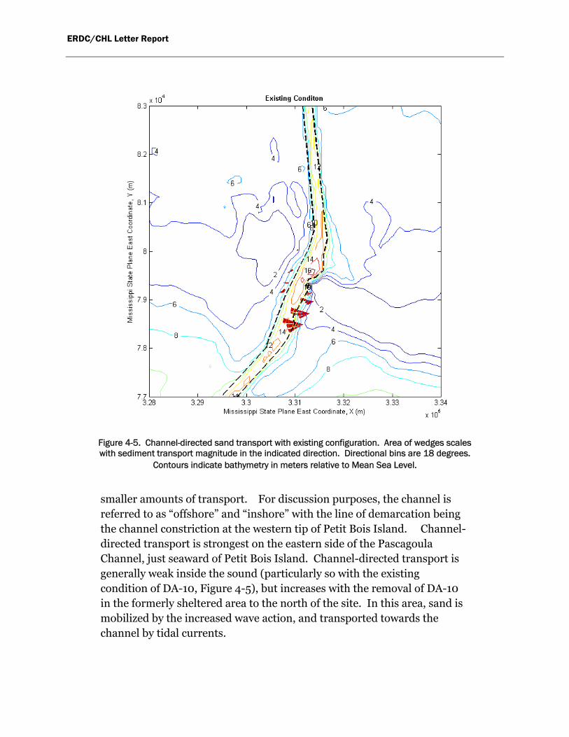
To this point, we have focused on changes in transport magnitude; however for channel sedimentation, direction is also important. Changes in directional transport were assessed adjacent to the navigation channel. Figures 4-5 and 4-6 present channel-directed transport roses for existing conditions and DA-10 removed, respectively. Each “wedge” in the rose represents cumulative transport for an 18 deg bin at each point, and any transport outside of a ±27 deg normal to the channel is excluded. Area of the colored wedge is scaled to transport potential. Therefore, large wedges indicate high transport in a specific direction while small wedges indicate
Figure 4-4. Ratio of sediment transport magnitude (removed/existing). Contours indicate bathymetry in meters relative to Mean Sea Level.
ERDC/CHL Letter Report
smaller amounts of transport. For discussion purposes, the channel is referred to as “offshore” and “inshore” with the line of demarcation being the channel constriction at the western tip of Petit Bois Island. Channel-directed transport is strongest on the eastern side of the Pascagoula Channel, just seaward of Petit Bois Island. Channel-directed transport is generally weak inside the sound (particularly so with the existing condition of DA-10, Figure 4-5), but increases with the removal of DA-10 in the formerly sheltered area to the north of the site. In this area, sand is mobilized by the increased wave action, and transported towards the channel by tidal currents.
Figure 4-5. Channel-directed sand transport with existing configuration. Area of wedges scales with sediment transport magnitude in the indicated direction. Directional bins are 18 degrees.
Contours indicate bathymetry in meters relative to Mean Sea Level.

ERDC/CHL Letter Report
The change in channel-directed transport between the two conditions was expressed as the ratio of transport with DA-10 removed to transport with existing conditions (Table 4-1). The values in Table 4-1 were determined from the sums of the channel-directed transport in each quadrant. For the offshore channel (south of the DA-10/Petit Bois constriction), transport on the west side of the channel was reduced to 60 percent of existing conditions with DA-10 removed, but transport on the east side of the channel increased by 10 percent. These changes in channel-directed transport are associated with the changes in flow patterns between Petit Bois Island and DA-10. With DA-10 removed, currents approaching the inlet are more aligned with the west side of the channel, but flood currents cross the eastern channel margin at a more oblique angle. Changes in sediment transport for the inshore channel (immediately north of the DA-10/Petit Bois constriction) are primarily influenced by the increased wave transmission with deepening of DA-10. Channel-directed transport on the
Figure 4-6. Channel-directed sand transport with DA-10 removed. Area of wedges scales with sediment transport magnitude in the indicated direction. Directional bins are 18 degrees.
Contours indicate bathymetry in meters relative to Mean Sea Level.

ERDC/CHL Letter Report
eastern side was unchanged, but increased by a factor of 60 (6000 percent) on the western side. The large value of transport ratio for the inshore/west region reflects the change from near-zero transport under the existing configuration to moderate transport with increased wave exposure. Considering all channel-directed transport along the channel margins, the removal of DA-10 results in 30 percent greater sand transport towards the channel.
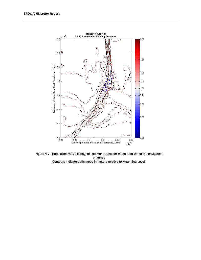
Horn Island Pass requires little dredging due to its high flow rate and high transport potential. Figure 4-7 presents the transport ratio of DA-10 removed to existing within the navigation channel. With DA-10 removed, transport potential between Petit Bois Island and DA-10 is 65 to 75 percent of existing in a 2.5 km (1.5 mi) reach of channel centered on the Petit Bois Island/DA-10 constriction. This reduction in sediment transport potential favors increased sedimentation, but whether the channel will shoal to a degree that requires dredging is undetermined. Net channel sedimentation is dependent upon the supply of sediment to the channel reach, and local sediment transport gradients. The channel sedimentation issue would be best evaluated through application of a mass conservative sediment transport model.
This screening-level sediment transport assessment suggests that removal of DA-10 could result in a 30 percent increase in channel-directed transport and a 25-35 percent decrease in transport capacity of the channel between Petit Bois Island and the DA-10 site. While the present analysis is insufficient to determine the response of this portion of the Pascagoula Channel or dredging requirements, the analysis does suggest that a closer examination of the sedimentation potential of this portion of channel is warranted.
Table 4-1: DA-10 removed to existing conditions channel-directed transport ratios
West East
Offshore 0.6 1.1
Inshore 60 No change
ERDC/CHL Letter Report
Figure 4-7. Ratio (removed/existing) of sediment transport magnitude within the navigation channel.
Contours indicate bathymetry in meters relative to Mean Sea Level.

ERDC/CHL Letter Report
5 Summary Within the scope of MsCIP, plans are being formulated to restore sediment to crucial areas along the Mississippi Barrier Islands. As part of this plan, a number of possible suitable sand sources have been identified. The dredged material disposal site DA-10 is one of these sand sources. In order to address the possible impacts of removing or altering DA-10, ERDC-CHL has undertake a study to examine the effect of removing DA-10 through numerical model analyses of waves, currents, and sediment transport potential.
Three representative locations north of DA-10 were studied to determine the localized wave effects due to the removal of DA-10. The maximum wave height during the simulated time period is approximated 1 m and the time-averaged mean wave height is approximately 0.5 m for the Existing conditions at three locations studied. Existing conditions, waves are physically obstructed by DA-10 and less wave energy is allowed to propagate into the Mississippi Sound. However, under the DA-10 Removal scenario, increased wave heights can be attributed to additional wave energy that is no longer dissipated by the material at DA-10 and these waves continue to propagate shoreward in its lee. The time-averaged wave height amplification is approximately 0.2 m for the 3 representative locations studied. The largest wave height increases are observed at and immediately leeward of DA-10, which was removed (degraded) to a subaqueous shoal for the DA-10 Removal scenario.
Hydrodynamic modeling using 2D ADCIRC and 3D CH3D was performed for existing conditions and with DA-10 removed. The results of these simulations show considerable increase in current speeds within the footprint of DA-10 removed; however, the impacts on current speed and direction within the Lower Pascagoula channel and Horn Island Pass are not significant. Near bottom current speeds and directions were provided for the sediment transport potential analysis.
The numerical sediment transport model GTRAN was applied to identify possible impacts of removing DA-10 to sedimentation in Pascagoula Channel. Waves calculated from STWAVE and currents calculated from CH3D from March 2 to June 14, 2010 were used to predict transport magnitudes and pathways in the study area.
ERDC/CHL Letter Report
GTRAN results showed that transport potential would increase at the DA-10 location and in the area in the lee of DA-10. Transport in the lee of DA-10 is low with existing conditions and the area is sheltered by DA-10 from wave energy. Higher transport rates were predicted in this area with removal of DA-10 due to increased exposure to wave energy and less sheltering. Conversely, GTRAN results showed that less transport occurs in the channel between DA-10 and Petit Bois Island with DA-10 removed.
This screening-level sediment transport assessment suggests that the complete removal of DA-10 could result in a 30 percent increase in channel-directed transport and a 25-35 percent decrease in transport capacity of the channel between Petit Bois Island and the DA-10 site. While the present analysis is insufficient to determine the response of this portion of the Pascagoula Channel or dredging requirements, the analysis does suggest that a closer examination of the sedimentation potential of this portion of channel is warranted if sedimentation quantities are required.

ERDC/CHL Letter Report
References
Amante, C., and Eakins, B.W., 2009. ETOPO1 1 Arc-Minute Global Relief Model: Procedures, Data Sources and Analysis. NOAA Technical Memorandum NESDID NGDC-24, 19 pp.
Brock, J., Wright, W., Nayegandhi , A., Patterson, M., Wilson, I and Travers, L., 2007. EAARL Topography-Gulf Islands National Seashore-Mississippi. USGS Open File Report 2007-1377.
Bunch, B. W., Channel, M., Corson, W. D., Ebersole, B. A., Lin, L., Mark, D. J., McKinney, J. P., Pranger, S. A., Schroeder, P. R., Smith, S. J., Tillman, D. H., Tracy, B. A., Tubman, M. W., and Welp, T. L. 2003. “Evaluation of Island and Nearshore Confined Disposal Facility Alternatives, Pascagoula River Harbor Dredged Material Management Plan,” Technical Report ERDC-03-3, U.S. Army Engineer Research and Development Center, Vicksburg, MS.
Bunch, B. W., Corson, W. D., Ebersole, B. A., Mark, D., J., McKinney, J. P., Tillman, D. H., and M. W. Tubman. 2005. “Evaluation of Gulfport Navigation Channel Alternatives, Gulfport Reevaluation Report (GRR),” Technical Report ERDC-TR-XX-X, U.S. Army Engineer Research and Development Center, Waterways Experiment Station, Vicksburg, MS.
Bunya, S., Dietrich, J.C., Westerink, J.J., Ebersole, B.A., Smith, J.M., Atkinson, J.H., Jensen, R., Resio, D.T., Leuttich, R.A., Dawson, C., Cardone, V.J., Cox, A.T., Powell, M.D., Westerink, H.J, and Roberts, H.J., 2010. A High-Resolution Coupled Riverine Flow, Tide, Wind, Wind Wave, and Storm Surge Model for Southern Louisiana and Mississippi. Part I – Model Development and Validation. Monthly Weather Review, 138, pg. 345-377.
Buster, N.A., and Morton, R.A., 2011, Historical bathymetry and bathymetric change in the Mississippi-Alabama coastal region, 1847–2009: U.S. Geological Survey Scientific Investigations Map 3154, 13 p. pamphlet.

ERDC/CHL Letter Report
Chapman, R. S., Johnson, B. H., and S. R. Vemulakonda. 1996. “Users Guide for the Sigma Stretched Version of CH3D-WES; A Three-Dimensional Numerical Hydrodynamic, Salinity and Temperature Model,” Technical Report HL-96-21, U.S. Army Engineer Waterways Experiment Station, Vicksburg, MS.
Chapman, R. S., Luong, P. V, and M. W. Tubman. 2006. “Mississippi Sound Hydrodynamic and Salinity Sensitivity Modeling”. Final Report prepared for U. S. Army District, Mobile, Mobile, AL.
Cox, A.T. and V.J. Cardone, 2007. Workstation Assisted Specification of Tropical Cyclone Parameters from Archived or Real Time Meteorological Measurements. 10th International Workshop on Wave Hindcasting and Forecasting and Coastal Hazard Symposium, North Shore,Hawaii, November 11-16, 2007.
Gailani, J. Z., S. J. Smith, and N. C. Kraus. 2003. “Monitoring dredged material disposal at the mouth of the Columbia River, Washington/Oregon, USA”. ERDC/CHL TR- 03-5. Vicksburg, MS: U.S. Army Engineer Research and Development Center.
Hayter, E. J., and R. S. Chapman, 2011. “Users Guide for the Sigma Stretched Version of CH3D-SEDZLJ; A Three-Dimensional Numerical Hydrodynamic, Salinity, Temperature, and Sediment Transport Model,” Technical Report ERDC/CHL TR-11-X, U.S. Army Engineer Research and Development Center, Coastal and Hydraulics Laboratory, Vicksburg, MS.
IPET, 2007. Performance Evaluation of the New Orleans and Southeast Louisiana Hurricane Protection System. U.S. Corps of Engineers http://ipet.wes.army.mil
Jones, C.A., and Lick, W., 2001. “SEDZLJ: A Sediment Transport Model,” Final Report. University of California, Santa Barbara, California.
Komen, G. J., L. Cavaleri, M. Donelan, K. Hasselmann, S. Hasselmann, and P. A. E. M. Janssen, 1994, Dynamics and Modelling of Ocean Waves, 532 pp., Cambridge Univ. Press, New York..

ERDC/CHL Letter Report
Luettich, R. A., Jr., Westerink, J. J., and N. W. Scheffner. 1992. “ADCIRC: An Advanced Three-Dimensional Circulation Model for Shelves, Coasts, and Estuaries,” Technical Report DRP-92-6, U.S. Army Engineer Waterways Experiment Station, Vicksburg, MS.
Madsen, O. S., and P. N. Wikramanayake. 1991. “Simple models for turbulent wave-current bottom boundary layer flow”. Contract Report DRP-91-1. Vicksburg, MS: U.S. Army Engineer Waterways Experiment Station.
Meyer-Peter, E., and R. Müller. 1948. “Formulas for bed-load transport”. Second International Association of Hydraulic Engineering and Research (IAHR) Congress, Stockholm, Sweden. Delft, Netherlands: IAHR.
Mukai, A.Y., J.J. Westerink, R.A. Luettich, and D. Mark. 2002. “Eastcoast 2001, A tidal constituent database for Western North Atlantic, Gulf of Mexico, and Carribean Sea.” ERDC/CHL TR-02-24, U.S. Army Corps of Engineers Engineer Research and Development Center, Vicksburg, MS.
NOAA National Geophysical Data Center, NGDC Coastal Relief Model, Retrieved 01 December 2008, http://www.ngdc.noaa.gov/mgg/coastal/coastal.html
Nielsen, P., 1992. “Coastal Bottom Boundary Layers and Sediment Transport”. World Scientific Publishing, Singapore, Advanced Series on Ocean Engineering, vol. 4.
Ris, R.C., Holthuijsen, L.J., and Booij, N., J., 1999. A third generation wave model for coastal regions 2. Verification. Geophys. Res., 104, C4, 7667–7681.
Romeiser, R., 1993. Global validation of the wave model WAM over a 1-year period using Geosat wave height data, J. Geophys. Res., 98, 4713–4726.
Smith, J.M., Sherlock, A.R., and Resio, D.T., 2001. STWAVE: Steady-State Spectral Wave Model User’s Manual for STWAVE, Version 3.0. USACE Engineer Research and Development Center, Technical Report ERDC/CHL SR-01-1, Vicksburg, MS 80 pp.
Smith, J.M., 2007. Full-Plane STWAVE II: Model Overview. ERDC TN-SWWRP, U.S. Army Engineer Research and Development Center, Vicksburg, MS.
ERDC/CHL Letter Report
Smith, J.M., Jensen, R.E., Kennedy, A.B., Dietrich, C.J., and Westerink, J.J.W., 2010. Waves in Wetlands: Hurricane Gustav. Proceedings from the 32nd International Conference on Coastal Engineering. Shanghai, China, June 30-July 5, 2010.
Snir, M. Otto, S, Huss-Lederman, S, Walker, D, and J. Dongarra, 1998. “MPI - The Complete Reference: Volume 1, the MPI Core.” MIT Press, Cambridge, MA.
Soulsby, R.L., 1997. “Dynamics of Marine Sands.” Thomas Telford. London.
Van Rijn, L.C., 1984. “Sediment Transport: part I: bedload transport; part ii: suspended load transport: part iii: bed forms and alluvial roughness”, Journal of Hydraulic Engineering 110(10): 1431-1456; 110(11): 1613-1641, 110(12): 1733-1754.
Wamsley et al., 2011. Mississippi Coastal Improvement Program, Barrier Island Restoration Numerical Modeling, Technical Report ERDC/CHL TR-11-X, U.S. Army Engineer Research and Development Center, Coastal and Hydraulics Laboratory, Vicksburg, MS.
Wikramanayake, P.N., and Madsen, O.S., 1991.”Calculation of movable bed friction factors”, Tech. Rep. DACW-39-88-K-0047, 105 pp., CERC, U.S. Army Engineer Waterway Experiment Station, Vicksburg, MS., 1991.
Wikramanayake, P.N., and Madsen, O.S., 1994a. “Calculation of suspended sediment transport by combined wave-current flows.” Contract Report DRP-94-7, U.S. Army Engineer Waterway Experiment Station, Vicksburg, MS, USA.
Wikramanayake, P.N., and Madsen, O.S., 1994b. “Calculation of movable bed friction factors”. Contract Report DRP-94-5, U.S. Army Engineer Waterway Experiment Station, Vicksburg, MS, USA.
Zambreski, L., 1989. A verification study of the global WAM model, December 1987–November 1988, Tech. Rep. 63, Eur. Cent. for Medium-Range Weather Forecasts, Reading, England.
Zambreski, L., 1991. An evaluation of two WAM hindcasts for LEWEX, in Directional Ocean Wave Spectra, edited by R. C. Beal, pp. 167–172, Johns Hopkins Univ. Press, Baltimore, MD.
ERDC/CHL Letter Report
Appendix 1 – Time series of Current Speed, Direction and Differences Existing and Without DA-10
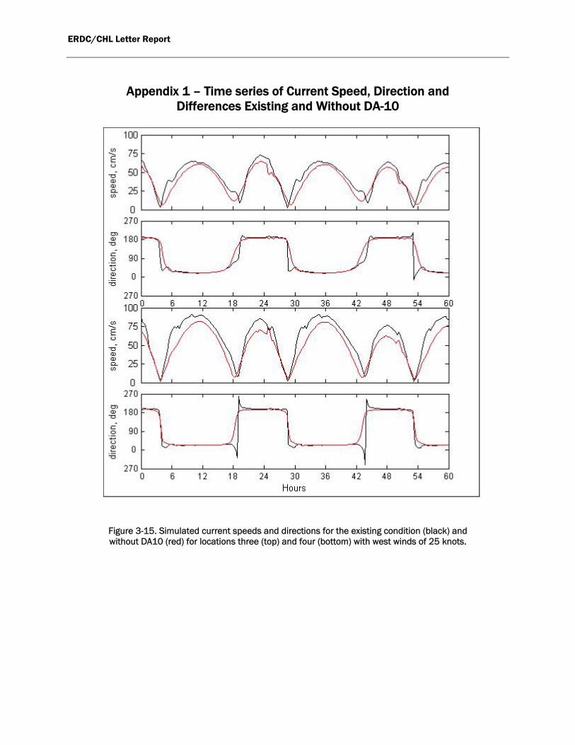
Figure 3-15. Simulated current speeds and directions for the existing condition (black) and without DA10 (red) for locations three (top) and four (bottom) with west winds of 25 knots.
ERDC/CHL Letter Report
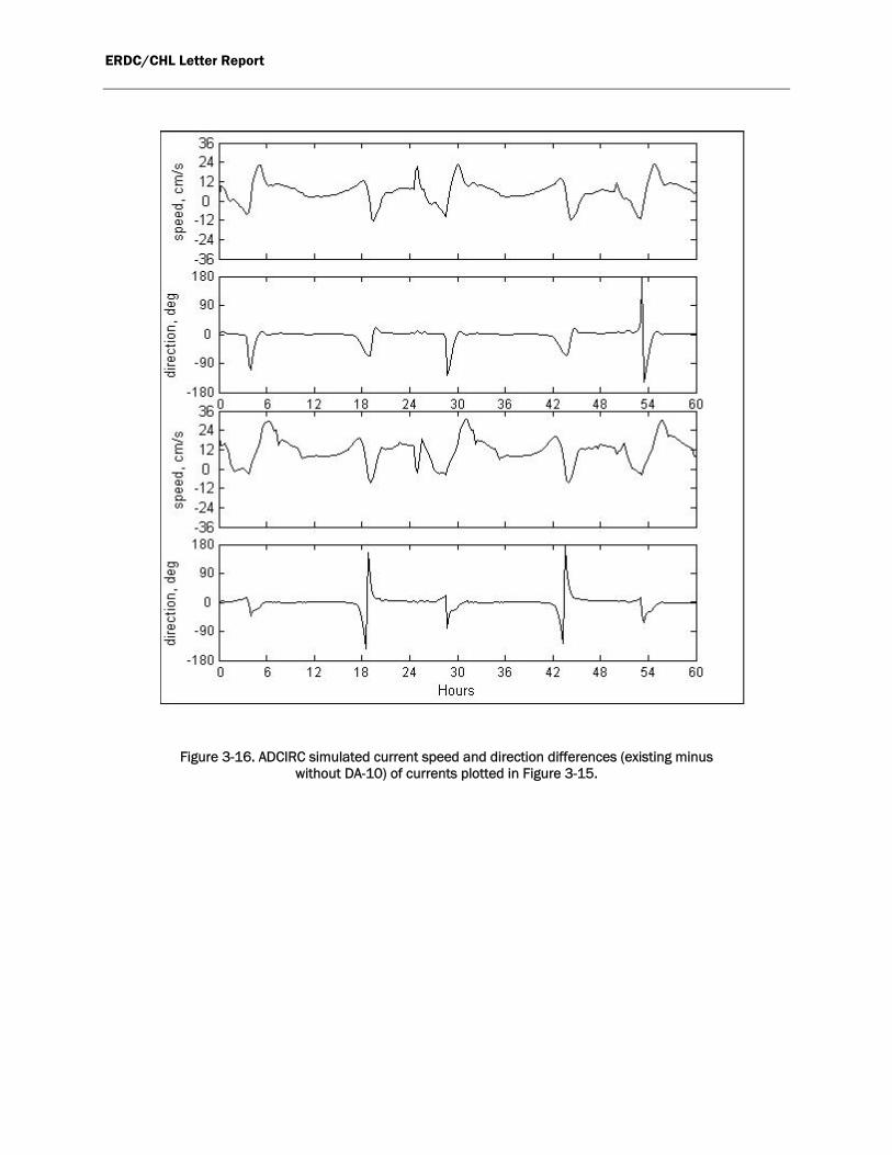
Figure 3-16. ADCIRC simulated current speed and direction differences (existing minus without DA-10) of currents plotted in Figure 3-15.
ERDC/CHL Letter Report
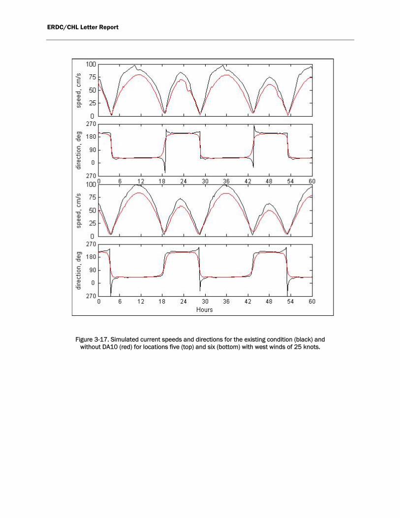
Figure 3-17. Simulated current speeds and directions for the existing condition (black) and without DA10 (red) for locations five (top) and six (bottom) with west winds of 25 knots.

ERDC/CHL Letter Report
Figure 3-18. ADCIRC simulated current speed and direction differences (existing minus without DA-10) of currents plotted in Figure 3-17.

ERDC/CHL Letter Report
Figure 3-19. Simulated current speeds and directions for the existing condition (black) and without DA10 (red) for locations seven (top) and eight (bottom) with west winds of 25 knots.

ERDC/CHL Letter Report
Figure 3-20. ADCIRC simulated current speed and direction differences (existing minus without DA-10) of currents plotted in Figure 3-19.

ERDC/CHL Letter Report
Figure 3-21. Simulated current speeds and directions for the existing condition (black) and without DA10 (red) for locations nine (top) and ten (bottom) with west winds of 25 knots.

ERDC/CHL Letter Report
Figure 3-22. ADCIRC simulated current speed and direction differences (existing minus without DA-10) of currents plotted in Figure 3-21.

ERDC/CHL Letter Report
Figure 3-23. Simulated current speeds and directions for the existing condition (black) and without DA10 (red) for location eleven with west winds of 25 knots.
Figure 3-24. ADCIRC simulated current speed and direction differences (existing minus without DA-10) of currents plotted in Figure 3-23.

ERDC/CHL Letter Report
Figure 3-25. Simulated current speeds and directions for the existing condition (black) and without DA10 (red) for locations one (top) and two (bottom) with south-southeast winds of 25
knots.

ERDC/CHL Letter Report
Figure 3-26. ADCIRC simulated current speed and direction differences (existing minus without DA-10) of currents plotted in Figure 3-25.

ERDC/CHL Letter Report
Figure 3-27. Simulated current speeds and directions for the existing condition (black) and without DA10 (red) for locations three (top) and four (bottom) with south-southeast winds of
25 knots.

ERDC/CHL Letter Report
Figure 3-28. ADCIRC simulated current speed and direction differences (existing minus without DA-10) of currents plotted in Figure 3-27.

ERDC/CHL Letter Report
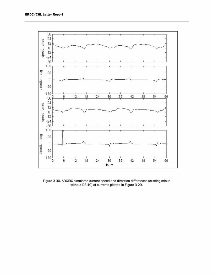
Figure 3-29. Simulated current speeds and directions for the existing condition (black) and without DA10 (red) for locations five (top) and six (bottom) with south-southeast winds of 25
knots.
ERDC/CHL Letter Report
Figure 3-30. ADCIRC simulated current speed and direction differences (existing minus without DA-10) of currents plotted in Figure 3-29.

ERDC/CHL Letter Report
Figure 3-31. Simulated current speeds and directions for the existing condition (black) and without DA10 (red) for locations seven (top) and eight (bottom) with south-southeast winds of
25 knots

ERDC/CHL Letter Report
Figure 3-32. ADCIRC simulated current speed and direction differences (existing minus without DA-10) of currents plotted in Figure 3-31.

ERDC/CHL Letter Report
Figure 3-33. Simulated current speeds and directions for the existing condition (black) and without DA10 (red) for locations nine (top) and ten (bottom) with south-southeast winds of 25
knots

ERDC/CHL Letter Report
Figure 3-34. ADCIRC simulated current speed and direction differences (existing minus without DA-10) of currents plotted in Figure 3-33.

ERDC/CHL Letter Report
Figure 3-35. Simulated current speeds and directions for the existing condition (black) and without DA10 (red) for location eleven with south-southeast winds of 25 knots
Figure 3-36. ADCIRC simulated current speed and direction differences (existing minus without DA-10) of currents plotted in Figure 3-35.