Final decision

Electricity transmission network service providers

Post-tax revenue model handbook

September 2007

© Commonwealth of Australia 2007

This work is copyright. Apart from any use permitted by the Copyright Act 1968, no part may be reproduced without permission of the Australian Competition and Consumer Commission. Requests and inquiries concerning reproduction and rights should be addressed to the Director Publishing, Australian Competition and Consumer Commission, GPO Box 3131, Canberra ACT 2601.

Australian Energy Regulator GPO Box 520 Melbourne Vic 3001

Ph: (03) 9290 1444 Fax: (03) 9290 1457 Email: AERInquiry@aer.gov.au

Amendment record

Version Date Pages

1 September 2007 24pp.

iii

Contents

Shortened forms ............................................................................................................ iv

1. Nature and authority............................................................................................ 1 1.1 Introduction.................................................................................................... 1 1.2 Authority ........................................................................................................ 1 1.3 Role of the model........................................................................................... 1 1.4 Confidentiality ............................................................................................... 1 1.5 Processes for revision .................................................................................... 1 1.6 Version history and effective date ................................................................. 1

2. The model .............................................................................................................. 2 2.1 Input sheet ...................................................................................................... 2

Opening regulated asset base ......................................................................... 4 Forecast real capital expenditure—as incurred.............................................. 5 Forecast real asset disposals—as incurred..................................................... 6 Forecast real net capital expenditure—as incurred........................................ 6 Forecast real capital expenditure—as commissioned .................................... 6 Forecast real asset disposals—as de-commissioned ...................................... 6 Forecast real net capital expenditure—as commissioned .............................. 6 Forecast real operating and maintenance expenditure ................................... 6 Cost of capital ................................................................................................ 7 Maximum allowed revenue for the current year............................................ 7 Energy delivered forecast .............................................................................. 7

2.2 WACC sheet .................................................................................................. 8 2.3 Assets sheet .................................................................................................... 9

Rolling forward the RAB and depreciation ................................................. 10 2.4 Analysis sheet .............................................................................................. 11

Building block approach to deriving cash flows.......................................... 13 Taxation and related costs and benefits ....................................................... 13 Cash flow analysis ....................................................................................... 14

2.5 Smoothing sheet........................................................................................... 16 2.6 Price path (nominal) sheet ........................................................................... 17 2.7 Price path (real) sheet................................................................................... 18 2.8 Chart 1–MAR sheet ..................................................................................... 18 2.9 Chart 2–Price path sheet .............................................................................. 19 2.10 Chart 3–Building Blocks sheet .................................................................... 20

iv

Shortened forms

ABBRR annual building block revenue requirement

AER Australian Energy Regulator

ATO Australian Tax Office

capex capital expenditure

CAPM capital asset pricing model

CPI consumer price index

IRR internal rate of return

MAR maximum allowed revenue

MWh megawatt hour

NEM National Electricity Market

NEMMCO National Electricity Market Management Company

NEL National Electricity Law

NER National Electricity Rules

NPV net present value

opex operating and maintenance expenditure

PTRM post-tax revenue model

PV present value

RAB regulated asset base

RFM roll forward model

TNSP transmission network service provider

WACC weighted average cost of capital

1

1. Nature and authority

1.1 Introduction

This handbook sets out the Australian Energy Regulator’s (AER) post-tax revenue model (PTRM) for electricity transmission network service providers (TNSPs). The PTRM is a series of Microsoft Excel spreadsheets developed in accordance with the requirements of clause 6A.5 of the National Electricity Rules (NER).

1.2 Authority

Clause 6A.5.2(a) of the NER requires the AER to develop and publish the PTRM, in accordance with the transmission consultation procedures.

1.3 Role of the model

The PTRM will be used by the AER to determine the maximum allowed revenue (MAR) to be earned by a TNSP over a regulatory control period. The TNSP uses the MAR to calculate the transmission prices to be paid by network users at each connection point in its network.

1.4 Confidentiality

The AER’s obligations regarding confidentiality and the disclosure of information provided to it by a TNSP are governed by the Trade Practices Act 1974, the National Electricity Law (NEL) and the NER.

1.5 Processes for revision

The AER may amend or replace the PTRM from time to time in accordance with clause 6A.5.2(b) of the NER and the transmission consultation procedures. A subsequent version of this handbook will accompany each new version of the PTRM.

1.6 Version history and effective date

A version number and an effective date of issue will identify each version of this handbook.

2

2. The model The PTRM is a set of Microsoft Excel spreadsheets that perform iterative calculations to derive a MAR for the next regulatory control period from a given set of inputs. The PTRM allows the user to vary the inputs to assess their impact on output data such as the MAR and other derived parameters.

The PTRM is configured to perform the calculations automatically whenever an input is recorded. If several inputs are to be recorded sequentially, the manual operation of the PTRM is recommended. In this case, Excel’s iteration mode of calculations needs to be selected. To do so, select Options from the Tools menu in Excel, then select the Calculations tab. Make sure that Manual (rather than Automatic) is selected and tick the iteration box.

When the manual mode is selected, a number of macros built in the PTRM (e.g. ‘Fix_Te’ and ‘Smooth’) will need to be operated manually. To run the macros, select Macro from the Tools menu, and then select Macros. To operate ‘Fix_Te’, highlight it and click on Run. To operate ‘Smooth’, highlight it and click on Run.

2.1 Input sheet

The Input sheet provides for key input variables to be entered in the PTRM. These are automatically linked to corresponding cells in the relevant sheets. Values should be entered into each cell that has light blue shading. This sheet has been split into eleven sections:

opening regulated asset base (RAB)

forecast real capital expenditure (capex)—as incurred

forecast real asset disposals—as incurred

forecast real net capex—as incurred

forecast real capex—as commissioned

forecast real asset disposals—as de-commissioned

forecast real net capex—as commissioned

forecast operating and maintenance expenditure (opex)

cost of capital

MAR for the current year

energy delivered forecast.

The input data must be recorded in the PTRM in a consistent format because the data is collected from TNSPs according to the AER’s submission guidelines.

3

Figure 1 provides an example of the Input sheet.

There is scope for making inputs into the other sheets. A few items may need to be specified outside of the Input sheet to capture a specific situation (e.g. tax loss carried forward in the Analysis sheet). These situations are addressed when they arise.

Figure 1: Input sheet

12345

6789

27

28293031323351

52535455565775

76777879808199

100101102103104105123

124125126127128129147

148149150151152153171

172173174175176177178179

180181182183184185186187188189190

191192193194

195196197198199

ABCD E F G H I J K L M N O P Q

Opening Asset Value

Assets Under Construction

Remaining Life

Standard Life

Opening Tax Value

Tax Remaining

Life

Tax Standard

Life

Base Financial

Year1,000.00 50.00 30.0 50.0 900.00 30.0 47.5 2007-08

800.00 20.00 30.0 50.0 700.00 30.0 47.5300.00 10.00 n/a n/a 200.00 n/a n/a

2,180.00 80.00 1,800.00

Year 2007-08 2008-09 2009-10 2010-11 2011-12 2012-13 2013-14 2014-15 2015-16 2016-1750.00 50.00 40.00 40.00 50.00 50.00 50.00 40.00 40.00 50.00 10.00 10.00 5.00 5.00 10.00

110.00 110.00 85.00 85.00 110.00 - - - - -

$ 500.00

Year 2007-08 2008-09 2009-10 2010-11 2011-12 2012-13 2013-14 2014-15 2015-16 2016-175.00 5.00 5.00 5.00 5.00 5.00 5.00 5.00 5.00 5.00 2.00 2.00 2.00 2.00 2.00

12.00 12.00 12.00 12.00 12.00 - - - - -

$ 60.00

Year 2007-08 2008-09 2009-10 2010-11 2011-12 2012-13 2013-14 2014-15 2015-16 2016-1745.00 45.00 35.00 35.00 45.00 - - - - - 45.00 45.00 35.00 35.00 45.00 - - - - - 8.00 8.00 3.00 3.00 8.00 - - - - -

98.00 98.00 73.00 73.00 98.00 - - - - -

$ 440.00

Year 2007-08 2008-09 2009-10 2010-11 2011-12 2012-13 2013-14 2014-15 2015-16 2016-1745.00 45.00 35.00 35.00 45.00 45.00 45.00 35.00 35.00 45.00 7.00 7.00 5.00 5.00 7.00

97.00 97.00 75.00 75.00 97.00 - - - - -

441.00$

Year 2007-08 2008-09 2009-10 2010-11 2011-12 2012-13 2013-14 2014-15 2015-16 2016-173.00 3.00 3.00 3.00 3.00 3.00 3.00 3.00 3.00 3.00 2.00 2.00 2.00 2.00 2.00 8.00 8.00 8.00 8.00 8.00 - - - - -

40.00$

Year 2007-08 2008-09 2009-10 2010-11 2011-12 2012-13 2013-14 2014-15 2015-16 2016-1742.00 42.00 32.00 32.00 42.00 - - - - - 42.00 42.00 32.00 32.00 42.00 - - - - - 5.00 5.00 3.00 3.00 5.00 - - - - -

89.00 89.00 67.00 67.00 89.00 - - - - -

401.00$

Year 2007-08 2008-09 2009-10 2010-11 2011-12 2012-13 2013-14 2014-15 2015-16 2016-1750.00 50.00 50.00 50.00 50.00 10.00 10.00 10.00 10.00 10.00 2.00 2.00 2.00 2.00 2.00 1.03 1.05 1.07 1.07 1.08 - - - - -

63.03 63.05 63.07 63.07 63.08 - - - - -

315.29$ Cost of Capital

Value6.00%3.00%1.10%6.00%

50.00%60.00%

1.000.08%

ValueCurrent Maximum Allowed Revenue 250.00

Year 2006-07 2007-08 2008-09 2009-10 2010-11 2011-12 2012-13 2013-14 2014-15 2015-16 2016-17Energy 26,000,000 27,000,000 28,000,000 29,000,000 30,000,000 31,000,000

Forecast Operating and Maintenance Expenditure ($m Real 2006-07)

Forecast Net Capital Expenditure – As Incurred ($m Real 2006-07)

Forecast Capital Expenditure – As Commissioned ($m Real 2006-07)

Forecast Asset Disposal – As De-Commissioned ($m Real 2006-07)

Forecast Net Capital Expenditure – As Commissioned ($m Real 2006-07)

Total

Utilisation of Imputation (Franking) Credits γProportion of Debt Funding D/VEquity Beta βe

Energy Delivered Forecast (MWh)

Maximum Allowed Revenue for 2006-07 ($m Nominal)

Nominal Risk Free Rate RfInflation Rate fDebt Risk Premium DRPMarket Risk Premium MRP

Debt Raising Cost Benchmark Dr

Input Variables

Forecast Capital Expenditure – As Incurred ($m Real 2006-07)

Forecast Asset Disposal – As Incurred ($m Real 2006-07)

Transmission linesSubstationsEasements

Easements

Transmission linesSubstations

Easements

Transmission linesSubstations

Easements

Opening Regulated Asset Base for 2007-08 ($m Nominal)

SubstationsEasements

Transmission lines

Total

Controllable opexCorporateEfficiency carryover

Total

Total

Total

Total

Total

Transmission linesSubstations

Debt raising costs

Asset Class NameTransmission linesSubstations

Transmission lines

Total

SubstationsEasements

Input cells are in blue

Easements

Asset Class 1Asset Class 2Asset Class 3

4

The PTRM can handle input data for up to a 10 year regulatory control period.1 The PTRM can be adjusted to account for regulatory control periods of longer duration.

The PTRM is configured to use the straight-line method as the default position for calculating depreciation. After consultation with the AER, TNSPs may propose that depreciation profiles other than the straight-line method be accommodated within the PTRM as part of pre-lodgement discussions and subject to satisfying the criteria in clause 6A.6.3(b) of the NER.

The PTRM is also configured to recognise capex on a partially as-incurred (hybrid) approach as the default position.2 After consultation with the AER, TNSPs may propose that a full as-incurred approach be accommodated within the PTRM as part of pre-lodgement discussions.

Opening regulated asset base

The opening RAB is the value of assets on which a return will be earned. The Input sheet requires a value for the opening RAB (broken into asset classes) at the start of the first year of the current regulatory control period. The RAB will fluctuate each year to reflect forecast capex (as-incurred), asset disposals and regulatory depreciation.

The recorded input values are linked to the Assets sheet, which also calculates depreciation for the regulatory control period. Notes have also been included for various cells with specific comments and explanations about the relevance of the inputs.

Asset class name

The asset classes/names are recorded in column G. It is important that the number of asset classes recorded in the RAB section matches the number of asset classes identified in the capex section. This allows the PTRM to model consistent depreciation across the asset classes.

The PTRM is configured to accommodate up to 20 asset classes.3 The number of asset classes used in the PTRM will vary between businesses. However, for each business the number of asset classes used in the PTRM must be consistent with that used in the AER’s roll forward model (RFM) to allow the closing RAB values determined in the RFM to be used as inputs to the opening RAB values in the PTRM.

Opening asset value

The opening asset values for each asset class are recorded in column J.

1 For a standard (shorter) regulatory control period, the input spaces that are not required should be

left blank or equal to zero. 2 The partially as-incurred method for recognising capex calculates the return on capital based on an

as-incurred approach and the return of capital (depreciation) is based on an as-commissioned approach.

3 The PTRM can be expanded to accommodate additional asset classes, when necessary.

5

Assets under construction

The value of assets under construction for each asset class is recorded in column K.4 These values should be consistent with those used in the RFM. The total value of assets under construction as at the end of the final year of the current regulatory control period (cell K27) is rolled into the opening RAB value (cell J27).

Remaining life

The remaining life of the asset classes is recorded in column L, based on the economic life of the assets.5

Standard life

The standard life of the asset classes is recorded in column M and measures how long the infrastructure would physically last had it just been built.

Opening tax value

The opening tax value for each asset class is sourced from the closing tax asset value for the current regulatory control period which has been determined in the RFM and is recorded in column N.

Tax remaining life

The remaining life of the asset classes for taxation purposes is recorded in column O based on the tax life specified by the Australian Tax Office (ATO) for the category of assets and commissioning date.

Tax standard life

The tax standard life of the asset classes is recorded in column P.

Base financial year

The financial year for the start of the next regulatory control period (year one) is recorded in cell Q7.

Forecast real capital expenditure—as incurred

Forecast capex (as-incurred) values for the next regulatory control period are recorded for each year in rows 31 to 50 (by asset class). Capex is rolled into the RAB when spending is incurred. Generally, capex falls into three broad categories:

asset augmentation (e.g. works to enlarge a network or to increase the capability of a network)

4 Inputs for assets under construction are only relevant for TNSPs moving from a full

as-commissioned approach to a partially as-incurred approach for recognising capex. 5 Generally assumed to be the weighted average remaining life of all individual assets in the class.

6

asset replacement (e.g. replacing assets that have passed their useful lives)

non-network asset (e.g. support the business expenditure)

These inputs are assumed to be in end of the year terms.

Forecast real asset disposals—as incurred

Forecast asset disposal (as-incurred) values are recorded for the year in which the disposal is expected to take place, in rows 55 to 74. These inputs are assumed to be in end of the year terms.

Forecast real net capital expenditure—as incurred

This section on forecast net capex does not require inputs to be recorded. For each asset class, forecast net capex is calculated based on the recorded forecast capex less forecast asset disposals. Forecast net capex (as-incurred) values are displayed in rows 79 to 98 and form part of the roll forward of the RAB in the Assets sheet. These inputs are assumed to be in end of the year terms.

Forecast real capital expenditure—as commissioned

Forecast capex (as-commissioned) values are recorded for each year in rows 103 to 122. These inputs are assumed to be in end of the year terms.

Forecast real asset disposals—as de-commissioned

The forecast de-commissioned asset values are recorded for each year in rows 127 to 146. These inputs are assumed to be in end of the year terms.

Forecast real net capital expenditure—as commissioned

This section on forecast net capex does not require inputs to be recorded. For each asset class, forecast net capex is calculated based on the recorded forecast capex less the value of de-commissioned assets. Forecast net capex (as-commissioned) values are displayed in rows 151 to 170 and are used to calculate depreciation in the Assets sheet. These inputs are assumed to be in end of the year terms.

Forecast real operating and maintenance expenditure

Opex typically includes items such as wages and salaries, leasing costs, costs associated with maintaining transmission assets, input costs and other service contract expenses paid to third parties. The forecast opex values for each year are recorded in rows 175 to 177, including any carryover amounts determined according to the efficiency benefit sharing scheme developed by the AER. Row 178 does not require inputs to be recorded because the calculation for benchmark debt raising cost is formula-driven and is based on the practice of treating the allowance as an opex line item. Additional opex inputs can be recorded by adding rows to this section—click on the button labelled Insert new row. These inputs are assumed to be in end of the year terms.

The forecast total opex values (row 179) are linked to the Analysis sheet.

7

Cost of capital

The cost of capital section (rows 183 to 189) records the following parameters:

nominal risk free rate

inflation rate

debt risk premium

market risk premium

gamma (utilisation of imputation (franking) credits)

proportion of debt funding

equity beta.

Each of these parameters is linked to the WACC sheet. The value or methodology for determining each parameter is specified in clause 6A.6.2 of the NER.6

The allowance for benchmark debt raising cost is also recorded in row 190. The value of the debt raising cost allowance is based on the notional debt issue size and is determined according to the methodology set out in Debt and equity raising transaction costs: Final report to the ACCC, a 2004 report by the Allen Consulting Group.

Maximum allowed revenue for the current year

Cell G194 records the current MAR for a TNSP. It is linked to the Price Path sheets and helps provide historical comparisons for forecast revenues over the next regulatory control period.

Energy delivered forecast

The energy delivered forecast section (row 198) records information, which is linked to the Price Path sheets. Energy delivered forecasts may be obtained from the most recent National Electricity Market Management Company statement of opportunities, a TNSP’s annual planning report or other relevant industry sources.

6 Clause 6A.5.3(b)(1) of the NER requires the AER to specify in the PTRM a methodology that is

likely to result in the best estimate of expected inflation. For the time being, the AER will use a range of indicators to guide it in determining the appropriate forecast inflation (see section 4.7 of AER, Final decision—Post-tax revenue model, September 2007). An inflation forecast of 3 per cent, based on this approach, provides the best estimate in the PTRM framework at this time (see AER, Draft decision—SP AusNet transmission network revenue cap 2008–09 to 2012-13, September 2007).

8

2.2 WACC sheet

The WACC sheet calculates the required return on equity, cost of debt and the weighted average cost of capital (WACC) using the relevant cost of capital parameters from the Input sheet.

The effective tax rates derived from the cash-flow analysis are also reported in the WACC sheet, including various measures of WACC calculated from the forecast cash-flows in the Analysis sheet. The nominal vanilla WACC (cell F27) is multiplied by the opening RAB in the Analysis sheet to determine the return on capital building block.

Figure 2 provides an example of the WACC sheet.

Figure 2: WACC sheet

12345

67891011121314151617181920212223242526272829303132333435

A B C D E F G H

Cost of Capital Parameters

Input Data & Calculated Inputs

Basic Building Block Model

Nominal Risk Free Rate Rf 6.00%Real Risk Free Rate Rrf 2.91%Inflation Rate f 3.00%Cost of Debt Margin DRP 1.10%Nominal Pre-tax Cost of Debt Rd 7.10%Real Pre-tax Cost of Debt Rrd 3.98%Market Risk Premium MRP 6.00%Corporate Tax Rate T 30.00%Effective Tax Rate for Equity (From Relevant Cashflows) Te 19.17% 19.17%Effective Tax Rate for Debt (Effective Debt Shield) Td 30.00% 30.00%Utilisation of Imputation (Franking) Credits γ 50.00%Proportion of Equity Funding E/V 40.00%Proportion of Debt Funding D/V 60.00%Equity Beta βe 1.00

WACC Analysis

Formula ApproximationPost-tax Nominal Return on Equity(pre-imp) 12.00% 12.00%Post-tax Real Return on Equity(pre-imp) 8.74% 8.74%Nominal Vanilla WACC 9.06% 9.06%Real Vanilla WACC 5.88% 5.88%Post-tax Nominal WACC 7.27% 8.52%Post-tax Real WACC 4.15% 5.36%Pre-tax Nominal WACC 9.57% 9.59%Pre-tax Real WACC 6.38% 6.40%Nominal Tax Allowance 0.51% 0.53%Real Tax Allowance 0.49% 0.51%

9

2.3 Assets sheet

The Assets sheet calculates the value of the RAB for each year over the next regulatory control period in real and nominal terms. It also calculates both regulatory and tax depreciation. The Assets sheet displays 55 years of data so that the effective tax rate can be estimated.

Figure 3 provides an example of the Assets sheet.

Figure 3: Assets sheet

123456789103152535455688194

316317318319320321322323324325326327328329342355368590591

A B C D E F G H I J K

Asset Roll Forward0 1 2 3 4 5

Year 2006-07 2007-08 2008-09 2009-10 2010-11 2011-12

Inflation Assumption (CPI % increase) 3.00% 3.00% 3.00% 3.00% 3.00% 3.00%Cumulative Inflation Index (CPI end period) 100% 103.0% 106.1% 109.3% 112.6% 115.9%

Opening Regulated Asset Base 2,180.0 Real Capex 100.8 100.8 75.1 75.1 100.8 Nominal Capex 103.9 107.0 82.1 84.5 116.9

Real Asset Values

Real Straight-line Depreciation 60.00 61.73 63.46 64.77 66.09 Transmission lines 33.3 34.2 35.1 35.7 36.4

Substations 26.7 27.5 28.4 29.1 29.7 Easements - - - - -

Real Residual RAB (end period) 2,180.0 2,220.8 2,260.0 2,271.6 2,282.0 2,316.7 Real Residual RAB (start period) - 2,180.0 2,220.8 2,260.0 2,271.6 2,282.0

Nominal Asset Values

Inflation on Opening RAB 65.4 68.6 71.9 74.5 77.1 Nominal Straight-line Depreciation 61.8 65.5 69.3 72.9 76.6 Nominal Regulatory Depreciation 3.6- 3.1- 2.6- 1.6- 0.4- Nominal Residual RAB (end period) 2,180.0 2,287.5 2,397.6 2,482.3 2,568.4 2,685.7 Inflated Nominal Residual RAB (start period) - 2,245.4 2,356.1 2,469.5 2,556.7 2,645.4

Nominal Tax Values

Tax Depreciation 53.3 55.2 57.0 58.5 60.0 Transmission lines 30.0 30.9 31.8 32.6 33.3

Substations 23.3 24.2 25.2 25.9 26.7 Easements - - - - -

Residual Tax Value (end period) 1,800.0 1,838.3 1,877.6 1,893.8 1,910.7 1,953.8

10

Rolling forward the RAB and depreciation

For consistency, the depreciation in a period must equal the difference between the RAB at the start and end of the period. Further, as depreciation is intended to represent the return of capital over the life of the asset, accumulated depreciation should not exceed the initial actual capital cost of the infrastructure.

The opening RAB and real forecast net capex values displayed in this sheet (rows 9 to 30) are sourced from the Input sheet. Nominal forecast net capex values are displayed in rows 31 to 51. The modelling of capex in the PTRM is based on a partially as-incurred approach. Under this approach the return on capital is calculated based on as-incurred forecast net capex and the return of capital (depreciation) is calculated based on as-commissioned forecast net capex.

Capex can be incurred evenly throughout the year and therefore it is reasonable to assume that on average it takes place half-way through the year. However, the PTRM calculates the return on capital based on the opening RAB for each year and capex is not added to the RAB until the end of the year in which the asset is incurred. To address this timing difference of modelling the real capex, a half-real vanilla WACC is provided (capitalised and recovered over the life of the assets) to compensate for the six-month period before capex is included in the RAB (rows 10 to 30).7

Real asset values are displayed in rows 55 to 317. Real straight-line depreciation is calculated in rows 55 to 315. It uses the opening RAB, forecast capex (as-commissioned) values and asset lives from the Input sheet. The individual depreciation profiles for each asset class can be viewed by expanding rows 56 to 315. The roll forward of the closing RAB in real terms for each year is calculated in row 316.

Nominal asset values are displayed in rows 321 to 325. To compensate the TNSP for inflation, the residual value of the RAB at the end of each year is adjusted upwards for the amount of expected inflation in that year. This adjustment is calculated in row 321. The change in the nominal value of the RAB from year to year in nominal terms is calculated by adjusting the closing RAB (row 324) for forecast net capex (as-incurred) and the regulatory depreciation allowance. Regulatory depreciation (row 323) is calculated as the nominal straight-line depreciation (row 322), less the inflation adjustment on the opening RAB (row 321).

Depreciation for tax purposes is calculated in rows 329 to 590 based on the tax asset values, net capex (as-commissioned) values and tax asset lives from the Input sheet. The individual tax depreciation profiles for each asset class can be viewed by expanding rows 330 to 589. Tax depreciation is calculated separately because asset values and asset lives for tax purposes generally differ from that for regulatory purposes.

7 The half-real vanilla WACC is calculated by the square root of (1 + real vanilla WACC) to account

for the compounding effect on an annual rate.

11

2.4 Analysis sheet

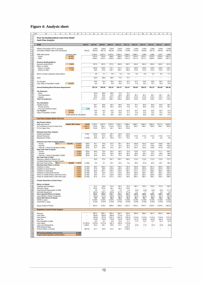
The Analysis sheet itemises the basic costs, or building blocks, of the TNSP, which are then added together to calculate the annual building block revenue requirement (ABBRR). In other words, the Analysis sheet is where the data from the Input sheet is combined with the calculations in the Assets and WACC sheets to estimate a TNSP’s revenue requirement. The Analysis sheet displays 55 years of data so that the effective tax rate can be estimated.

The Analysis sheet also includes an analysis of the forecast cash flows. This analysis provides rate of return measures estimated from forecast revenues and costs, including: expected post and pre-tax returns on equity, effective tax rates, the effective cost of debt and selected measures of the WACC.

Figure 4 below provides an example of the Analysis sheet.

12

Figure 4: Analysis sheet

123456789

101112131415161718192021222324252627282930313233343536373839404142434445464748495051525354555657585960616263646566676869707172737475767778798081828384858687888990919293949596979899100101102103104

A B C D E F G H I J K L M N O P

Post-Tax Building Block Cash Flow ModelCash Flow Analysis

Year 2006-07 2007-08 2008-09 2009-10 2010-11 2011-12 2012-13 2013-14 2014-15 2015-16 2016-17

Inflation Assumption (CPI % increase) 3.00% 3.00% 3.00% 3.00% 3.00% 3.00% 3.00% 3.00% 3.00% 3.00%Cumulative Inflation Index (CPI end period) 100.0% 103.0% 106.1% 109.3% 112.6% 115.9% 119.4% 123.0% 126.7% 130.5% 134.4%

RAB (start period) (nominal value) 2,180.0 2,287.5 2,397.6 2,482.3 2,568.4 2,685.7 2,685 2,682 2,677 2,669 - Equity 40.00% 872.0 915.0 959.0 992.9 1,027.3 1,074.3 1,074.1 1,073.0 1,070.8 1,067.5 - Debt 60.00% 1,308.0 1,372.5 1,438.6 1,489.4 1,541.0 1,611.4 1,611.2 1,609.5 1,606.2 1,601.3

Revenue Building BlocksNominal Vanilla WACC 9.06% 197.5 207.2 217.2 224.9 232.7 243.3 243.3 243.0 242.5 241.8 Return on Asset - Return on Equity 12.00% 104.6 109.8 115.1 119.1 123.3 128.9 128.9 128.8 128.5 128.1 - Return on Debt 7.10% 92.9 97.4 102.1 105.7 109.4 114.4 114.4 114.3 114.0 113.7

Return of Asset (regulatory depreciation) 3.6- 3.1- 2.6- 1.6- 0.4- 0.4 2.9 5.4 8.2 11.1

Opex 64.9 66.9 68.9 71.0 73.1 - - - - -

Tax Payable 16.8 18.2 19.6 20.9 22.2 23.7 24.6 25.5 26.3 27.2 Less Value of Imputation Credits 50.00% 8.4- 9.1- 9.8- 10.4- 11.1- 11.9- 12.3- 12.7- 13.2- 13.6-

Annual Building Block Revenue Requirement 267.25 280.09 293.34 304.74 316.47 255.60 258.43 261.20 263.88 266.48

Tax Expenses - Opex 64.9 66.9 68.9 71.0 73.1 - - - - - - Tax Depreciation 53.3 55.2 57.0 58.5 60.0 62.1 62.1 62.1 62.1 62.1 - Interest 92.9 97.4 102.1 105.7 109.4 114.4 114.4 114.3 114.0 113.7 Total Tax Expenses 211.1 219.5 228.1 235.2 242.6 176.5 176.5 176.3 176.1 175.8

Tax CalculationTaxable Income 56.1 60.6 65.3 69.5 73.9 79.1 82.0 84.9 87.8 90.7 - Pre-tax Income 56.1 60.6 65.3 69.5 73.9 79.1 82.0 84.9 87.8 90.7 - Tax Loss Carried Forward 0.00 - - - - - - - - - - Tax Payable 30.00% 16.8 18.2 19.6 20.9 22.2 23.7 24.6 25.5 26.3 27.2 Value of Imputation Credits 50.00% 8.4 9.1 9.8 10.4 11.1 11.9 12.3 12.7 13.2 13.6

(intermediate tax calculation) 16.8 18.2 19.6 20.9 22.2 23.7 24.6 25.5 26.3 27.2

Cash Flow Analysis Below This Line

Net Present ValuesRAB (start period) Project NPV Check (19.0) 2,180.0 2,287.5 2,397.6 2,482.3 2,568.4 2,685.7 2,685.3 2,682.4 2,677.0 2,668.8 PV for Returns on and of Asset Only 2,545.0 193.9 204.1 214.6 223.3 232.3 243.7 246.1 248.5 250.7 252.9 PV for Capex Only 384.0 103.9 107.0 82.1 84.5 116.9 - - - - -

Nominal Cash Flow AnalysisCapital Expenditure 2,180 103.9 107.0 82.1 84.5 116.9 - - - - - Interest Payments - 92.9 97.4 102.1 105.7 109.4 114.4 114.4 114.3 114.0 113.7 Repayment of Debt (1,308) 64.5- 66.1- 50.8- 51.7- 70.4- 0.2 1.7 3.3 4.9 6.6

Nominal Cash Flow to Equity Holders - Pre-tax Te = 19.17% 13.24% (872) 70.1 74.8 91.0 95.1 87.4 140.9 142.3 143.7 144.9 146.1 - Post-tax 10.70% (872) 53.2 56.7 71.4 74.3 65.3 117.2 117.7 118.2 118.6 118.9 - Post-tax + Value of Imputation Credits 12.00% (872) 61.7 65.8 81.2 84.7 76.3 129.1 130.0 130.9 131.8 132.5 Real Cash Flow to Equity - Pre-tax 9.95% (872) 68.0 70.5 83.3 84.5 75.4 118.0 115.7 113.4 111.1 108.7 - Post-tax 7.48% (872) 51.7 53.4 65.4 66.0 56.3 98.2 95.7 93.3 90.9 88.5 - Post-tax + Value of Imputation Credits 8.74% (872) 59.9 62.0 74.3 75.3 65.9 108.1 105.7 103.4 101.0 98.6 Net Cash Flow to DebtDeduction Utilised to Reduce Tax 92.9 97.4 102.1 105.7 109.4 114.4 114.4 114.3 114.0 113.7 Unutilised Deductions Carried Forward - - - - - - - - - - Net Cash Flow to Debt Td = 30.00% 4.97% (1,308) 0.5 2.1 20.7 22.4 6.2 80.3 81.8 83.3 84.7 86.2 Nominal Cash Flows to AssetsCashflow to Asset 9.59% (2,180) 98.5 106.2 142.3 149.2 126.4 255.6 258.4 261.2 263.9 266.5 Cashflow to Asset Post-tax 8.52% (2,180) 81.6 88.0 122.8 128.4 104.3 231.9 233.8 235.7 237.6 239.3 Cashflow to Asset Real 6.40% (2,180) 95.6 100.1 130.3 132.6 109.1 214.1 210.1 206.2 202.2 198.3 Cashflow to Asset Real Post-tax 5.36% (2,180) 79.2 83.0 112.3 114.0 89.9 194.2 190.1 186.1 182.1 178.0 Check on Vanilla WACC Cash Flow (nom) 9.06% (2,180) 90.0 97.1 132.6 138.8 115.4 243.7 246.1 248.5 250.7 252.9 Check on Vanilla WACC Cash Flow (real) 5.88% (2,180) 87.4 91.6 121.3 123.3 99.5 204.1 200.1 196.1 192.2 188.2

Further Dissection of Cash Flows

Return on EquityCashflow with Imputation 61.7 65.8 81.2 84.7 76.3 129.1 130.0 130.9 131.8 132.5 Add back Capex 103.9 107.0 82.1 84.5 116.9 - - - - - Less Nominal Depreciation of RAB 3.6 3.1 2.6 1.6 0.4 (0.4) (2.9) (5.4) (8.2) (11.1) Add Debt Repayment (64.5) (66.1) (50.8) (51.7) (70.4) 0.2 1.7 3.3 4.9 6.6 Gives Nominal Return to Equity 104.6 109.8 115.1 119.1 123.3 128.9 128.9 128.8 128.5 128.1 Less Inflation in Equity Component (26.2) (27.4) (28.8) (29.8) (30.8) (32.2) (32.2) (32.2) (32.1) (32.0) Gives Real Return to Equity 78.5 82.3 86.3 89.4 92.5 96.7 96.7 96.6 96.4 96.1 %ROE (1 year) 12.00% 12.00% 12.00% 12.00% 12.00% 12.00% 12.00% 12.00% 12.00% 12.00%%real ROE (1 year) 8.74% 8.74% 8.74% 8.74% 8.74% 8.74% 8.74% 8.74% 8.74% 8.74%

Equity at Start of Period 872.0 915.0 959.0 992.9 1,027.3 1,074.3 1,074.1 1,073.0 1,070.8 1,067.5

Regulatory Control Period Analysis

Revenue - 267.2 280.1 293.3 304.7 316.5 255.6 258.4 261.2 263.9 266.5 Less Opex - (64.9) (66.9) (68.9) (71.0) (73.1) - - - - - Less Interest (92.9) (97.4) (102.1) (105.7) (109.4) (114.4) (114.4) (114.3) (114.0) (113.7) Less Tax - (16.8) (18.2) (19.6) (20.9) (22.2) (23.7) (24.6) (25.5) (26.3) (27.2) Plus Imputation Credits - 8.4 9.1 9.8 10.4 11.1 11.9 12.3 12.7 13.2 13.6 Less Capex (2,180.0) (103.9) (107.0) (82.1) (84.5) (116.9) - - - - - Less Loan Repayments 1,308.0 64.5 66.1 50.8 51.7 70.4 (0.2) (1.7) (3.3) (4.9) (6.6) RAB Residual Value 1,074.3 - - - - - Post-tax Return on Equity (872.0) 61.7 65.8 81.2 84.7 1,150.6 - - - - -

IRR (during regulatory control period) 12.00%Target (during regulatory control period) 12.00%

13

Building block approach to deriving cash flows

Clause 6A.5.4 of the NER requires the AER to apply the building block approach to assess the revenues required by a TNSP to recover the full cost of providing the regulated (prescribed) service. The revenue requirement includes a commercial return on its investment.

The key building blocks are:

the return on capital comprising (row 15):

the post tax return on equity (row 17)

the cost of debt (or the interest payments incurred) required to service borrowings (row 18)

the regulatory depreciation or return of capital (row 20)

opex (row 22)

net tax liabilities payable (the figure is net in the sense that it is the annual tax payable by the TNSP (row 24) less the value of imputation credits available to investing shareholders (row 25)).

The costs are determined for each year of the next regulatory control period to derive the ABBRR (row 27). As costs can fluctuate from year to year, the revenue requirement is smoothed over the regulatory control period to give the MAR (see section 2.5).

Taxation and related costs and benefits

Tax is payable on revenue less tax costs recognised by the ATO. Tax-deductible costs include interest or debt servicing, depreciation allowances and opex (rows 30 to 32).

Spreadsheet calculations

Tax payable by the TNSP for each year is calculated in rows 30 to 41, in three steps:

1. Pre-tax income is calculated as the ABBRR less the estimated total tax expense (row 37).

2. Tax loss carried forward is calculated (row 38).

3. Taxable income (row 36) is then the sum of the above.

The tax costs (rows 30 to 32) used in calculating the pre-tax income for the year are the same as those in the building blocks (rows 18 and 22) with the exception of depreciation. In the case of the building blocks, regulatory depreciation (row 20) is calculated based on the economic life of the asset (see rows 55 to 315 and 321 to 323 of the Assets sheet). Tax depreciation is generally based on a much shorter tax life or calculated in a different way (see rows 329 to 589 of the Assets sheet).

14

The tax payable is recognised as a building block cost and added to the revenue building blocks (row 24). Offsetting this tax cost is the benefit shareholders receive from imputation credits (gamma). This offsetting benefit is equal to gamma multiplied by the tax payable and is recorded in rows 25 and 40.

Cash flow analysis

Cash flow analysis is fundamental to the AER’s revenue determinations. It provides a comprehensive check on the validity of revenue determinations to ensure that the outcomes are consistent with the assumptions forming the basis of the building block approach. The Analysis sheet is designed to check the desired rate of return on equity that can be expected from the regulated revenue stream.

Net present values

The total returns on and of capital (comprising the RAB and capex) is calculated in row 47. The present value (PV) for these cash flows at the start of the first year of the next regulatory control period is calculated in cell F47. The PV for capex is calculated in cell F48. The PV can be used to show that the PTRM is providing the correct returns to the asset. The project net present value (NPV) check (cell F46) for the RAB should be equal to zero, which indicates that the asset is receiving the correct returns. Note that the NPV check on the returns is only relevant for depreciable assets (i.e. not applicable to easements).

Net cash flows available to equity holders

Net nominal pre-tax cash flows to equity holders (row 56) are represented by nominal revenues less:

opex

capex

interest payments

any repayment of debt in the period.

Net nominal post-tax cash flow to equity holders (row 57) is obtained by further deducting the tax expense of the business. Row 58 adds back the value of imputation credits to calculate the net post-tax benefits available to equity holders in a period.

The internal rate of return (IRR) of the net cash flows over the life of the assets is calculated in column E. The key IRR is the net post-tax returns to equity holders inclusive of imputation credits (re), as that is conceptually the return indicated by the capital asset pricing model (CAPM) calculation. The CAPM determined re should be validated by the estimated cash flows (row 58).

The corresponding real cash flows and the respective IRRs are calculated in rows 60 to 62.

15

The difference in the IRR applying to pre-tax and post-tax cash flows to equity allows the effective rate of tax (Te = 1 – rpost/rpre) to be calculated (cell D56). This can then be used as an input to the formula-based WACC calculations.

It is important to note that the formula-based WACC calculations will only provide an approximation of the actual WACC outcomes implied by the cash flow calculations. In practice, Te is substantially below the corporate tax rate for assets that can be depreciated at a faster rate for tax purposes.

Net cash flows necessary to service debt and the effective debt shield

The cost of debt is reduced by the value of the ‘debt shield’ (row 64) in calculating tax liabilities. Where the interest expense in a year reduces taxable income by a corresponding amount, the net cost of debt for investors is reduced by the corporate tax rate.

However, where the taxable income is so low that the full interest deduction is not required to reduce tax liabilities to zero, the value of the debt shield benefit is deferred to a later period. This effect is analysed in rows 64 to 66. That part of interest expense used to defer tax is calculated in each period (row 64) and the unused part carried forward is embodied in the tax loss carried forward calculation (row 65). This allows the net cost to the firm of paying debt holders, after taking account of the tax concession, to be calculated.

The IRR calculation (cell E66) represents the effective cost of debt, which is generally well below the nominal cost of debt based on the current interest rates.

Nominal cash flows to assets and calculation of WACC estimates

The cash flows to the different sources of capital (debt and equity) have been presented above, but the cash flows to the assets as a whole are of interest since these aggregate numbers characterise the nature of the regulated business.

The IRRs from these cash flows are the WACC estimates expected from the application of the regulatory framework and have greater validity than any formula-based approximations. They are summarised in the WACC sheet along with the formula-based approximations. It should be noted that the WACC outcomes are calculated for reporting purposes only. They are not required for setting revenues since the modelling already provides the requisite revenue forecasts.

Regulatory control period analysis

Rows 92 to 103 provide an additional analysis of the cash flow to equity holders over a regulatory control period.

The purpose of this section is to confirm that the desired re target remains over the regulatory control period. Rows 92 to 103 are essentially an expansion of the calculations used to derive row 58—that is, cash flow to equity holders inclusive of the value of imputation credits.

16

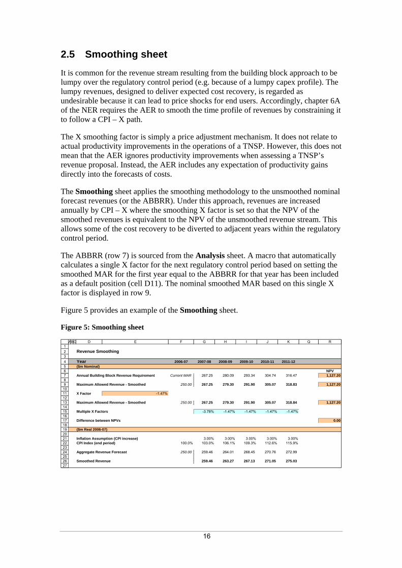
2.5 Smoothing sheet

It is common for the revenue stream resulting from the building block approach to be lumpy over the regulatory control period (e.g. because of a lumpy capex profile). The lumpy revenues, designed to deliver expected cost recovery, is regarded as undesirable because it can lead to price shocks for end users. Accordingly, chapter 6A of the NER requires the AER to smooth the time profile of revenues by constraining it to follow a CPI – X path.

The X smoothing factor is simply a price adjustment mechanism. It does not relate to actual productivity improvements in the operations of a TNSP. However, this does not mean that the AER ignores productivity improvements when assessing a TNSP’s revenue proposal. Instead, the AER includes any expectation of productivity gains directly into the forecasts of costs.

The Smoothing sheet applies the smoothing methodology to the unsmoothed nominal forecast revenues (or the ABBRR). Under this approach, revenues are increased annually by CPI – X where the smoothing X factor is set so that the NPV of the smoothed revenues is equivalent to the NPV of the unsmoothed revenue stream. This allows some of the cost recovery to be diverted to adjacent years within the regulatory control period.

The ABBRR (row 7) is sourced from the Analysis sheet. A macro that automatically calculates a single X factor for the next regulatory control period based on setting the smoothed MAR for the first year equal to the ABBRR for that year has been included as a default position (cell D11). The nominal smoothed MAR based on this single X factor is displayed in row 9.

Figure 5 provides an example of the Smoothing sheet.

Figure 5: Smoothing sheet

123456789

101112131415161718192021222324252627

ABC D E F G H I J K Q R

Revenue Smoothing

Year 2006-07 2007-08 2008-09 2009-10 2010-11 2011-12($m Nominal)

NPVAnnual Building Block Revenue Requirement Current MAR 267.25 280.09 293.34 304.74 316.47 1,127.20

Maximum Allowed Revenue - Smoothed 250.00 267.25 279.30 291.90 305.07 318.83 1,127.20

X Factor -1.47%

Maximum Allowed Revenue - Smoothed 250.00 267.25 279.30 291.90 305.07 318.84 1,127.20

Multiple X Factors -3.78% -1.47% -1.47% -1.47% -1.47%

Difference between NPVs 0.00

Inflation Assumption (CPI increase) 3.00% 3.00% 3.00% 3.00% 3.00%CPI Index (end period) 100.0% 103.0% 106.1% 109.3% 112.6% 115.9%

Aggregate Revenue Forecast 250.00 259.46 264.01 268.45 270.76 272.99

Smoothed Revenue 259.46 263.27 267.13 271.05 275.03

($m Real 2006-07)

17

A TNSP may nominate the X factor to apply for each year (inputs at row 15) of the next regulatory control period. These X factors may differ from year to year subject to satisfying the requirements of the NER.

Clause 6A.6.8 requires X factors to be set such that:

1. The NPV of the expected smoothed MAR (cell R9 or R13) must equal the NPV of the expected ABBRR (cell R7).

2. The expected smoothed MAR for the final year of the regulatory control period must be as close as reasonably possible to the ABBRR for that year.

A TNSP’s nominated X factors may be recorded in row 15 and the buttons in row 17 can be used to ensure that the NPVs of the smoothed and unsmoothed revenue streams are equal—that is, the difference between the NPVs is zero (cell R17). Based on this approach, the nominal smoothed MAR is displayed in row 13.

The Smoothing sheet also calculates the expected ABBRR and smoothed MAR in real terms (rows 24 and 26) by taking the nominal revenues and dividing by the inflation forecast over the next regulatory control period.

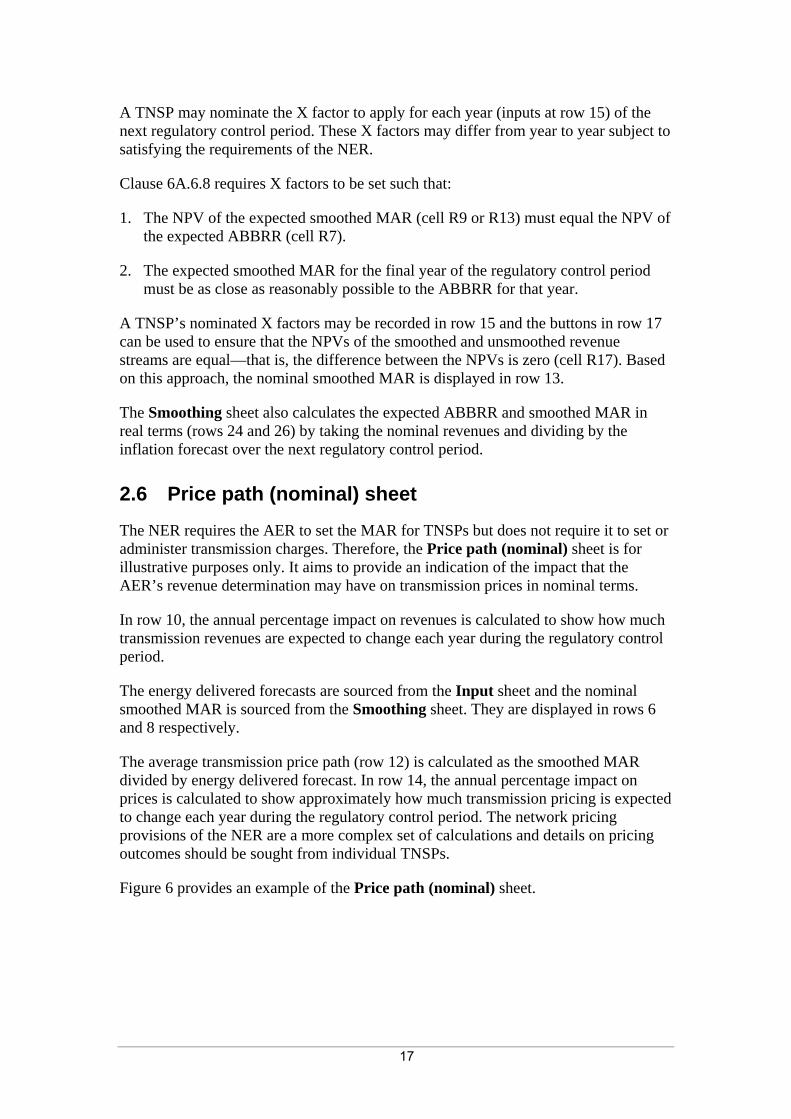
2.6 Price path (nominal) sheet

The NER requires the AER to set the MAR for TNSPs but does not require it to set or administer transmission charges. Therefore, the Price path (nominal) sheet is for illustrative purposes only. It aims to provide an indication of the impact that the AER’s revenue determination may have on transmission prices in nominal terms.

In row 10, the annual percentage impact on revenues is calculated to show how much transmission revenues are expected to change each year during the regulatory control period.

The energy delivered forecasts are sourced from the Input sheet and the nominal smoothed MAR is sourced from the Smoothing sheet. They are displayed in rows 6 and 8 respectively.

The average transmission price path (row 12) is calculated as the smoothed MAR divided by energy delivered forecast. In row 14, the annual percentage impact on prices is calculated to show approximately how much transmission pricing is expected to change each year during the regulatory control period. The network pricing provisions of the NER are a more complex set of calculations and details on pricing outcomes should be sought from individual TNSPs.

Figure 6 provides an example of the Price path (nominal) sheet.

18

Figure 6: Price Path (nominal) sheet

12345678910111213141516

A B C D E F G H I J K Q R S

Price Path Analysis

Year 2006-07 2007-08 2008-09 2009-10 2010-11 2011-12

Energy (MWh) 26,000,000 27,000,000 28,000,000 29,000,000 30,000,000 31,000,000

Smoothed Revenue ($m Nominal) 250,000,000 267,246,304 279,302,786 291,903,181 305,072,028 318,834,970

Annual Percentage Impact on Revenues 6.90% 4.51% 4.51% 4.51% 4.51% Total 24.94%Average 4.99%

Price Path ($/MWh) 9.62$ 9.90$ 9.98$ 10.07$ 10.17$ 10.28$

Annual Percentage Impact on Prices 2.94% 0.78% 0.91% 1.03% 1.14% Total 6.79%Average 1.36%

2.7 Price path (real) sheet

The Price path (real) sheet is set up in a similar manner to the Price path (nominal) sheet except that the transmission prices are calculated in real terms.

Figure 7 provides an example of the Price path (real) sheet.

Figure 7: Price Path (real) sheet

12345678910111213141516

A B C D E F G H I J K Q R S

Price Path Analysis

Year 2006-07 2007-08 2008-09 2009-10 2010-11 2011-12

Energy (MWh) 26,000,000 27,000,000 28,000,000 29,000,000 30,000,000 31,000,000

250,000,000 259,462,431 263,269,663 267,132,762 271,052,545 275,029,846

Annual Percentage Impact on Revenues 3.78% 1.47% 1.47% 1.47% 1.47% Total 9.65%Average 1.93%

Price Path ($/MWh) 9.62$ 9.61$ 9.40$ 9.21$ 9.04$ 8.87$

Annual Percentage Impact on Prices -0.06% -2.16% -2.03% -1.91% -1.81% Total -7.97%-1.59%

Smoothed Revenue ($m Real 2006-07)

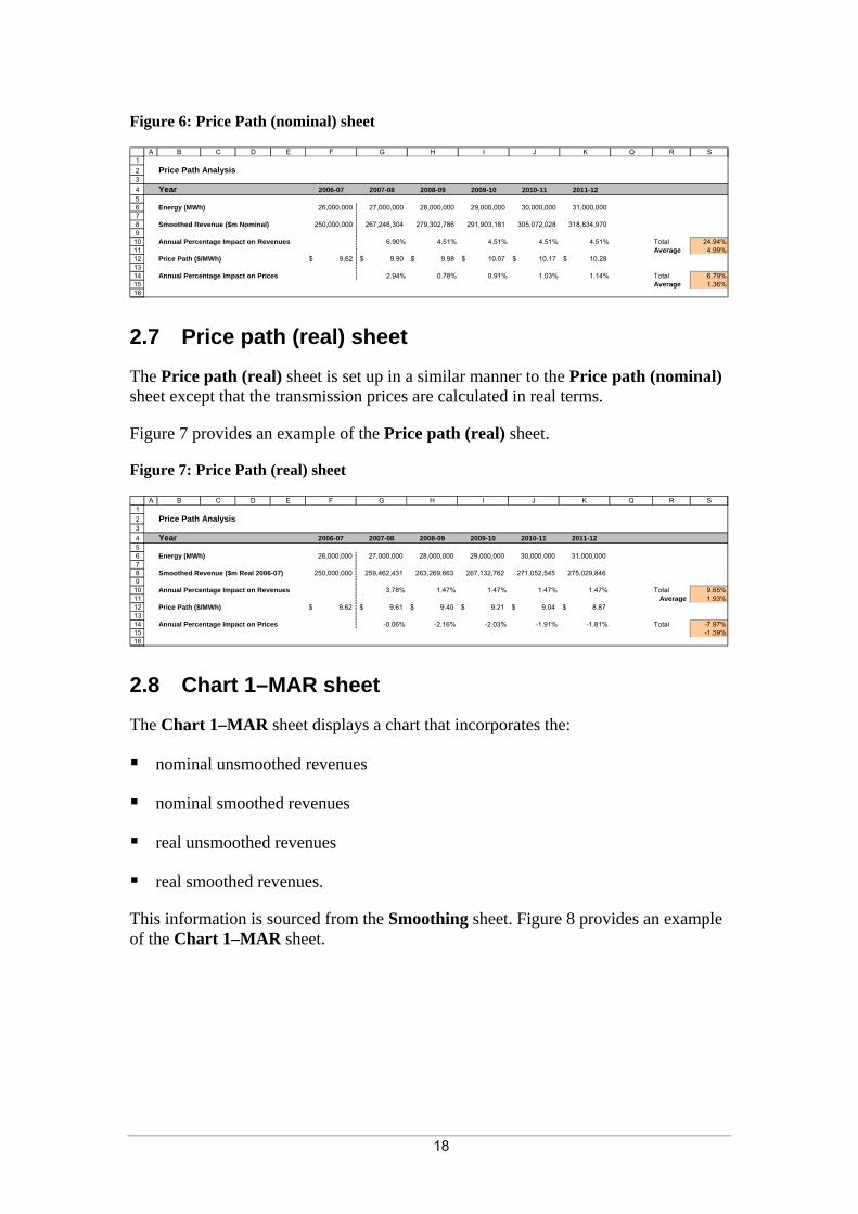
2.8 Chart 1–MAR sheet

The Chart 1–MAR sheet displays a chart that incorporates the:

nominal unsmoothed revenues

nominal smoothed revenues

real unsmoothed revenues

real smoothed revenues.

This information is sourced from the Smoothing sheet. Figure 8 provides an example of the Chart 1–MAR sheet.

19

Figure 8: Chart 1–MAR

Chart 1 - Smoothing of the Maximum Allowed Revenue

$100

$150

$200

$250

$300

$350

$400

2006-07 2007-08 2008-09 2009-10 2010-11 2011-12

Year

($m

)

Nominal unsmoothed revenueNominal smoothed revenueReal unsmoothed revenueReal smoothed revenue

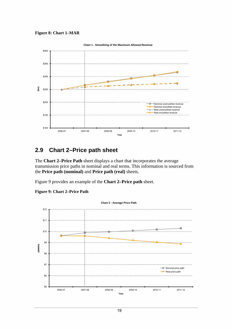
2.9 Chart 2–Price path sheet

The Chart 2–Price Path sheet displays a chart that incorporates the average transmission price paths in nominal and real terms. This information is sourced from the Price path (nominal) and Price path (real) sheets.

Figure 9 provides an example of the Chart 2–Price path sheet.

Figure 9: Chart 2–Price Path

Chart 2 - Average Price Path

$5

$6

$7

$8

$9

$10

$11

$12

2006-07 2007-08 2008-09 2009-10 2010-11 2011-12

Year

($/M

Wh)

Nominal price pathReal price path

20

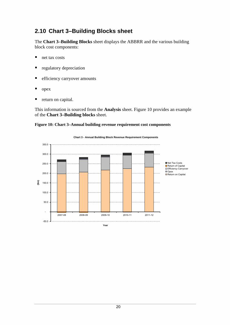
2.10 Chart 3–Building Blocks sheet

The Chart 3–Building Blocks sheet displays the ABBRR and the various building block cost components:

net tax costs

regulatory depreciation

efficiency carryover amounts

opex

return on capital.

This information is sourced from the Analysis sheet. Figure 10 provides an example of the Chart 3–Building blocks sheet.

Figure 10: Chart 3–Annual building revenue requirement cost components

Chart 3 - Annual Building Block Revenue Requirement Components

-50.0

-

50.0

100.0

150.0

200.0

250.0

300.0

350.0

2007-08 2008-09 2009-10 2010-11 2011-12

Year

($m

)

Net Tax CostsReturn of CapitalEfficiency CarryoverOpexReturn on Capital