Appendix B

Emissions Inventory Methodology

THIS PAGE INTENTIONALLY LEFT BLANK

B - 1

I. EMISSIONS INVENTORY DEVELOPMENT FOR CARGO HANDLING EQUIPMENT

A. Overview Cargo handling equipment can be a significant source of diesel particulate matter (PM) emissions in communities near ports and intermodal rail facilities. To reduce diesel particulate matter (PM) emissions in these communities CARB passed a regulation requiring reductions in emissions from cargo handling equipment. With proposed amendments to that regulation staff is updating the inventory with a wealth of new information collected since 2005. These new sources of information include the regulatory reporting data which provides an accounting of all the cargo handling equipment (CHE) in the state including their model year, horsepower and activity. In addition, the Ports and Los Angeles and Long Beach have been conducting annual emissions inventories, and a number of the major rail yards and other ports in the state have completed individual emissions inventories. The methodology discussed here reflects updated population and activity, the impact of the recession on growth, and engine load. Emissions estimates were developed for six equipment classes associated with California’s 14 ports 16 and intermodal rail yards. The updated inventory and emissions model, Cargo Handling Emissions Inventory Model, or CHEI, and the CHEI Working Files are posted on ARB’s web site at http://www.arb.ca.gov/ports/cargo/cheamd2011.htm. (ARB, 2011f), (ARB,2011o)

B. Methodology for Estimating Emissions The emissions from each type of equipment covered by the CHE regulation are calculated using the following equation:

Emissions = Pop * HP * LF * Activity * EF Where:

Pop = Equipment population HP = Maximum rated horsepower (hp) LF = Load factor Activity = Activity or annual operation (hr/yr) EF = Emission factor (g/hp-hr)

The equation above is applied to each piece of equipment, and the results summed to provide the emissions inventory. To estimate emissions in future years, staff projects a baseline population of vehicles into the future by modeling turnover and purchasing characteristics. These projections are modeled in a Microsoft Access database that projects future populations and emissions based

B - 2

on location-specific characteristics and behavior, economic forecasts, and ARB’s regulatory requirements. This forecasting module is described in detail in chapter III of this appendix. The baseline inventory and the inputs to the equation above are described in section I.C below.

C. Emissions Inventory Inputs

1. Population After the CHE rule was adopted in December, 2005, the regulation required all ports and rail yards with applicable vehicles to submit equipment inventories to ARB by January 31, 2007. (ARB, 2005c) The reporting forms required information such as vehicle make, model and serial number, and also usage characteristics such as hours used and average load factor during operation. These reports provided a new inventory of equipment for 2006 that serves as a baseline population for the updated inventory model. The equipment population estimated for the original inventory developed in 2005 was based on a survey of ports and rail yards that ARB distributed in December, 2004 and a separate survey in 2001 and 2002 from the Port of Los Angeles and Port of Long Beach. (ARB, 2005b) The equipment population at the ports of Los Angeles and Long Beach represent over half of the population of cargo handling equipment in California. The combined surveys provided information on approximately 2,000 pieces of equipment, and the results were scaled upwards to estimate the total population of equipment in the state. This updated inventory is based on regulatory reporting data that accounts for all equipment in the state and therefore requires no scaling. ARB received equipment reports from 72 companies that operate at the 14 ports and 16 rail yards covered by the regulation. Table I-1 details the count of equipment reported by facility.

Table I-1: Population of Equipment by Facility

Location Port/Rail Population Port of Los Angeles P 1424 Port of Long Beach P 1307 Port of Oakland P 600 BNSF Los Angeles R 274 Port of Stockton P 145 Port of Hueneme P 96 UPRR ICTF R 86 BNSF San Bernardino R 83

B - 3

Location Port/Rail Population San Diego Port & Railyard P 66 Port of San Francisco P 61 UPRR LA/Commerce R 51 Port of Richmond P 48 UPRR Oakland R 35 BNSF Stockton R 33 UPRR LATC R 29 Port of Sacramento P 28 BNSF Oakland R 26 UPRR Lathrop R 23 BNSF Commerce R 22 UPRR City of Industry R 20 Port of Redwood City P 20 BNSF Fresno R 9 Other Bay Area Ports & Railyards P 8 BNSF Richmond R 4 Port of Humboldt Bay P 19 Total 4517 Table I-2 and Table I-3 show the combined population of equipment in ports and rail yards, respectively, and compares the totals against the original inventory population estimates for calendar year 2006.

Table I-2: Calendar Year 2006 Equipment Population for All Ports

Equipment Type Original Inventory

Updated Inventory

Yard Tractor 2115 1861 Forklift 461 712

Container Handling Equipment 529 500

Crane 278 (All Cranes)

253 (RTG Only)

Construction Equipment 134 192

Other General Industrial Equipment 41 149

Total 3558 3667

B - 4

Table I-3: Equipment Population for All Rail Yards

Equipment Type Original Inventory

Updated Inventory

Yard Tractor 326 507

Crane 82 (All Cranes)

89 (RTG Only)

Forklift 24 66

Container Handling Equipment 30 25

Other General Industrial Equipment 5 15

Construction Equipment 1 3

Total 468 705 As shown in the preceding tables, the updated population for ports is very close to the original inventory estimates, only 2 percent higher overall. The population for rail yards, however, is 51 percent higher than the original inventory. This new data provided not only an updated count of equipment, but also allowed staff to improve the inventory with updated location-specific characteristics, such as equipment age. Table I-4 compares the updated average age of equipment based on the reporting data against the averages age from the original inventory. The data shown for the original inventory below is the averages ages in 2006. Because the baseline for the original inventory was calendar year 2004, the averages in the table are shown after the impact of two years of attrition predicted by the original inventory model. This comparison is useful in showing the difference in the expected average age of equipment in the original inventory and the average ages from the reporting data. The significant difference seen in expected average and the average age reported to ARB not only impacts the baseline population, but also lead to revised projections of turnover and vehicle purchasing that more closely model real world conditions.

B - 5

Table I-4: Average Equipment Age by Type in Calendar Year 2006

Equipment Type Original Inventory

Updated Inventory

Yard Tractor 3.6 4.6 Forklift 4.1 12.7 Container Handling Equipment 5.2 5.9

Crane 7 6.7 (RTG Only)

Construction Equipment 5.4 13.6 Other General Industrial Equipment 4.6 13.1 Total 4.2 7.1

Overall, the updated inventory demonstrates a minor increase in overall population, but a shift to a significantly older average vehicle age.

2. Turnover

Turnover is a function that describes the relationship between equipment age and the proportion of equipment that has been removed from the port or rail yard fleet. These vehicles may leave a specific port/rail yard because of scrappage or because they are being sold to another fleet. The function is expressed in terms of a fraction of vehicles by age that remains in the population. The average lifetime varies by the type of equipment and the location. For this updated inventory staff relied on the turnover rate curves as defined by U.S. Environmental Protection Agency (U.S. EPA). (USEPA, 2005) U.S. EPA provides equations for which the user defines the useful life and maximum age of the equipment. Useful life is defined as the age where 50% of the vehicles have been turned over and the maximum life is the age at which all the vehicles have left the specific port or rail yard fleet. The application of these turnover functions was tailored to align with our understanding of the useful life information included in the reporting data.

In order to reflect location-specific turnover characteristics staff developed useful life and maximum life inputs based on groups of fleets with similar average age equipment. For example, all yard tractor at ports and rail yards with an average age around 5 years follow the same turnover trends whereas yard tractor fleets with an average around 10 years follow their own turnover trend. This way, smaller fleets which are difficult to model can follow the trends of similarly-aged larger ones. The assumption is that equipment with similar averge age will have the same turnover rates. The categorizations for these groupings can be found in Appendix A.

B - 6

Turnover rates follow a traditional s-curve, but the shape of the curve is defined by the useful life and maximum life. Based on the age distributions developed from the grouped data in the table above staff identified the useful life as 1.5 times the average age of the equipment. The maximum age was defined as the 98th percentile of the age distribution. The following graphs are examples of the s-curves for RTG cranes with an average age of 6 and forklifts with an average age of 21. As you can see for this example location, RTG cranes are generally turned over by age 10. In the other example location, forklifts are maintained until almost 35 years old.

Figure I-1: Example Turnover Rates for Cranes and Forklifts

B - 7

Turnover Curve Development The turnover functions, or s-curve, developed for this updated inventory are specific to individual locations and equipment type characteristics and were developed in three steps: (1) Group similar fleets into the same category; (2) Develop a Business As Usual (BAU) age distribution; (3) Stretch or compress the curve so turnover models the BAU distribution. The result is that locations with a similar average age will follow the turnover rates. (1) Group similar fleets into the same category Since some equipment types at ports and rail yards have small populations, staff grouped locations with similar characteristics together. Different equipment types, however, were never modeled using the same turnover rates since the data shows that the different CHE equipment types are too unique to have the same turnover assumptions. Locations that were grouped together were based on average vehicle age into a (L)ow, (M)edium, (H)igh, or (O)ver-high category (see Appendix A). For example, all the equipment given a ‘High’ average age designation are used to develop the same BAU age distribution, which will be discussed in more detail later. (2) Develop a Business As Usual (BAU) age distribution Once the categories have been established, many different sources of population data are compiled to develop an age distribution that represents business as usual in the absence of the regulation. To develop this BAU age distribution staff relied on the regulatory reporting database (ARB, 2005c), the annual inventories for the Port of Los Angeles/Port of Long Beach (Starcrest, 2010a) (Starcrest 2010b), the 2005 Port of Oakland inventory (Environ, 2008), the 2005 Railyard Health Risk Assessment inventories (ARB, 2008), and ARB’s 2004 CHE equipment survey. (ARB, 2005b) The BAU age distributions were developed from a polynomial fit of the data. These curves are then used for turnover and purchasing and are unique to each category of equipment type shown in Appendix A. (3) Stretch or compress the curve so turnover models the BAU distribution The useful life of the turnover function was determined to be at 1.5 times the average age of the BAU distribution because this is where the distributions had a significant drop off in population. It was also observed that the model preserved BAU well at this useful life. The max life was placed at the 98th percentile of the population data. Any equipment that was reported older than this had a very large standard deviation from what was normal; increasing the max age to include these outliers would result in a population much older than anticipated.

B - 8

3. Purchasing The other component of equipment turnover is purchasing. Purchasing is very specific to each port and rail yard. Some locations maintain vehicles that are very young and thus purchase young vehicles while other maintain older equipment and thus purchase older vehicles. Since the updated inventory developed for these amendments is location-group and equipment-specific purchasing behavior was necessary at this level of detail. In order to establish purchasing habits for each location-group an historically average baseline age distribution was developed. This distribution, hereby referred to as the ‘business as usual age distribution’ was estimated from 2001-2007 historical equipment inventory data (see Turnover Curve Development above). This age distribution represents the age distribution of the equipment at that location in the absence of the rule and recession. This distribution was used as a target age distribution in projecting fleet turnover in the absence of the recession and regulation. The distribution of vehicle purchases was determined by the business as usual age distribution for the baseline inventory. New vehicle purchases under the rule inventory were dictated by the rule requirements. The example for yard trucks below helps to illustrate the concept. The blue line is the 2006 age distribution. After attrition is applied the resulting population (the dark green line with boxes) is a year older and smaller as a result of vehicles leaving the fleet (turnover). To determine the age of vehicles purchased the business as usual (BAU) age distribution is used to distribute new vehicle purchases among the ages where the attrited 2007 population is below the business as usual population. These purchases are added to the 2007 attrited population resulting in the 2007 grown population (light green line with triangles). In reality this adjustment takes into account both purchasing and necessary modifications to turnover rates where the estimated turnover assumptions don’t exactly match fleet behavior. Over time the base year age distribution will move towards resembling the business as usual age distribution.

B - 9

Figure I-2: Purchasing Example for 2006 to 2007 population change

Purchasing Distribution After turnover has been applied to a given population purchasing is distributed among model years to eventually reestablish the BAU age distribution. These purchases enter the fleet at a specific location as a result of turnover and growth and are accomplished in two steps: (1) Calculating the number of total vehicles that need to be purchased; and (2) Distributing the purchases so the BAU distribution is eventually reestablished. (1) Calculating the number of total vehicles that need to be purchased The total number of vehicles that need to be purchased is a function of the number retired and the expected growth from one year to the next. The growth of a population is calculated by multiplying the count of equipment before retirement by a growth factor (see ‘6. Growth & Recovery’ for details on growth factors). (2) Distributing the results so the BAU distribution is reestablished into the future The total number of vehicles purchased is distributed among model years so that each age bin gets relatively closer to the BAU distribution. If an age bin is already above the BAU distribution there is no purchasing for that bin. The percentage of vehicles given to each bin is chosen so that each gets proportionally closer to BAU. For example, if 3 vehicles are to be distributed between age 3 and age 5 which have populations of 8 and 10 respectively, and BAU has these populations

B - 10

both at 12 vehicles, then the age 3 bin gets 2 vehicles and age 10 bin gets 1 vehicle.

4. Engine Load Factor

Engine load is the average operational level of an engine in a given application as a fraction or percentage of the engine manufacturer’s maximum rated horsepower. Since emissions are directly proportional to engine horsepower, load factors are used in the inventory calculations to adjust the maximum rated horsepower to normal operating levels.

In 2006 the Port of Los Angeles and Port of Long Beach conducted a study of engine load for yard trucks. (Starcrest, 2008a) (Starcrest, 2008b) In 2009, a similar study was performed for cranes operated at both ports. (Starcrest, 2010a) (Starcrest, 2010b) Both studies demonstrated that the load factor used in the original inventory was too high. The result was that the load factor for yard trucks was reduced to 0.39, and to 0.2 for RTG cranes. Load factors for excavators were updated from 0.57 to 0.55, as excavators were combined with the ‘Tractor/Loader/Backhoe’ category into the ‘Construction Equipment’ category of CHE, with a shared load factor of 0.55. Table I-5 below displays the load factor in the original inventory and the updated load factors.

In the original inventory, the load factors for each equipment type were taken from the ARB OFFROAD model. (ARB, 2007) For all other CHE equipment types except yard trucks and RTG cranes this remains the best available data.

Table I-5: Engine Load Factors

Equipment Original Inventory Updated Inventory Yard Tractor 0.65 0.39 RTG Crane 0.43 0.2 Excavator 0.57 0.55

Forklift 0.30 0.30 Material Handling Equip 0.59 0.59

Other General Industrial Equip 0.51 0.51 Tractor/Loader/Backhoe 0.55 0.55

B - 11

5. Activity

Background The activity or annual operation of off-road equipment is measured in annual average hours of use and varies by equipment type and age. Since the original rulemaking a number of new data sources have become available. These data show, Figures I-3 and I-4 below, that there are differences in activity by location as well as differences in activity as the equipment ages. These differences have been analyzed and taken into account in this updated inventory. Activity profiles for CHE in the original rulemaking inventory were estimated using data from a CARB survey of ports and rail yards in 2004. (ARB, 2004) Activity data were collected from 69 owner/operators statewide and captured operating hours for approximately 2,000 pieces of equipment. These data were aggregated to represent typical activity of specific equipment types at ports and rail yards as shown in Table I-6.

Table I-6: Activity Values for CHE in Original Inventory

Equipment Type Port Rail YardCrane 1371 1632

Excavator 2222 1162Forklift 1098 803

Material Handling Equip 2388 2388Other General Industrial Equip 693 1632

Sweeper/Scrubber 872 872Tractor/Loader/Backhoe 755 755

Yard Tractor 2536 1289

Annual Hours

B - 12

Figure I-3: Yard Truck Annual Hours by Location (2006)

0

1000

2000

3000

4000

5000

6000

RY 1

RY 2

RY 3

RY 4

RY 5

RY 6

RY 7

Port

1

RY 8

RY 9

RY 1

0

Port

2

RY 1

1

Port

3

RY 1

2

RY 1

3

Port

4

Port

5

Port

6

Port

7

Port

8

Annu

al H

ours

Port Yard Trucks (Original)

RY Yard Trucks (Original)

Figure I-4: Activity by Age for Yard Tractors in a California Port

0

1000

2000

3000

4000

5000

6000

7000

0 5 10 15 20 25 30 35

Age (years)

Ann

ual H

ours

Data Sources Since the original CHE emissions inventory was developed in 2005, new data sources for CHE activity have become available. These new data sources are

B - 13

the basis for the activity values in the new emissions inventory and are described below. CHE Regulation Reporting Data: As part of the 2006 CHE regulation, fleet owners and operators of CHE were required to submit information to CARB regarding equipment populations and hours of use. (ARB, 2005) Data were collected for over 4,000 pieces of equipment. Rail Yard Health Risk Assessments (HRA): As part of the rail yard emission reduction program, health risk assessments were initiated in 2005 to determine the relative risk of exposure to diesel particulate matter in the proximity of 17 intermodal rail yards. As part of the assessment, activity data were collected for over 400 pieces of cargo handling equipment. (ARB, 2008) Starcrest/ENVIRON Port Emissions Inventories: CHE emissions inventories for the past several years have previously been developed by the Starcrest consulting group for the Ports of Los Angeles, Long Beach and San Diego. In addition, the ENVIRON consulting group developed a CHE emissions inventory for the Port of Oakland in 2005. (Environ, 2008) As part of the emission inventory development process, activity data for several thousand pieces of equipment were collected at each of these ports. For the current inventory, calendar year 2006 activity data from these consulting reports were used as new sources of activity data. (Starcrest, 2008a) (Starcrest, 2008b) (Starcrest, 2008c)

Methodology Depending on the equipment type and location, staff used either one of two methods to develop activity profiles. For those locations where use was determined to be a function of age an appropriate activity profile was developed. For those locations where activity was not determined to be a function of age an average activity was employed. These two methods are described below. Trend Method: For this method, staff identified those equipment types displaying a significant decreasing trend in activity by age. Significant decreasing trends were identified by plotting all the available activity data described previously for each equipment type and location and performing a linear regression. The trend was considered significant it the slope was negative (i.e. decreasing activity by age) and contained a t-value greater than the critical t value at the 95% confidence level. In these cases, the trend line equation was used to calculate the activity by age profile for the specific equipment type and location. In order to ensure that the activity values never became zero due to the decreasing trend line, staff determined an inflection point (i.e. age) where activity ceased to decrease and became constant. The first step was to identify the age

B - 14

that represented twice the average age of the equipment types in a given location. Staff then calculated the average activity of all available data for the specific equipment type above this age. The point at which the decreasing trend line intersected this activity value was then used to define the activity by age profile for the specific equipment type and location. Figure I-5 shows an example activity by age profile for yard tractors at the Port of Los Angeles using the new methodology as well as the activity by age profile in the previous inventory.

Figure I-5: Activity by Age Profile for POLA Yard Tractors

0

500

1000

1500

2000

2500

3000

3500

Act

ivit

y (h

ours

/yea

r)

Age (years)

Updated

Original

Average Method: For those equipment types where there was no significant trend, the average of all activity values was assigned to specific equipment type and location. In other words, one activity value was assigned to the equipment type regardless of how old the equipment was.

Results Using the above methodologies, staff calculated the overall average hours by equipment type. The results are shown in Tables I-7 and I-8 for ports and rail yards, respectively. For comparison purposes, the average activity values used in the previous emissions inventory are also shown.

B - 15

Table I-7: Average Activity Values at Ports

Original Inventory (for 2006) Updated Inventory (2006)Equipment Type (hours/year) (hours/year)

Construction Equipment 1,084 1,497Container Handling Equipment 2,388 1,884

Forklift 1,098 701Other General Industrial Equipment 693 1,265

RTG Crane 1,371 1,574Yard Tractor 2,536 2,020

All Equipment 2,159 1,656

Table I-8: Average Activity Values at Rail Yards

Original Inventory (for 2006) Updated Inventory (2006)Equipment Type (hours/year) (hours/year)

Construction Equipment 755 141Container Handling Equipment 2,388 1,705

Forklift 803 2,234Other General Industrial Equipment 1,632 1,024

RTG Crane 1,632 3,398Yard Tractor 1,289 4,627

6. Growth & Recovery The growth factors used to estimate cargo handling equipment emissions in future years was based on growth factors from ARB’s Ocean-Going vessel (OGV) inventory for container, bulk, general and reefers vessels. Information on these growth factors can be found in the OGV technical appendix. (ARB, 2011l) The economic recession that officially started in December of 2007 and ended in June 2009 was the most severe since the Great Depression, and had a severe impact on industries throughout California. To forecast activity following the recession, three recovery scenarios were considered to encompass the possible rates of growth of “fast”, “slow”, and “average”. The fast recovery scenario assumes that total activity would return to projected historically average levels in 2017 and then grow at the historical average rate. A return to trend by 2017 was based on the Congressional Budget Office forecast which indicated that real gross domestic product at a nationwide level will converge with potential gross domestic product trends no later than 2015. This forecast was modified with the assumption that California’s recovery will lag the nation by several years, yielding the 2017 recovery date assumed for the fast recovery scenario. For the slow recovery scenario, staff assumed that activity would be permanently depressed relative to historical levels, but continue to grow at historical rates. The average scenario is the average of the fast and slow scenarios. The impact of the recession was estimated from port call and TEU data. Given the uncertainty in forecasting emissions after such a deep recession, staff relied

B - 16

on the average recovery scenario. This scenario, for the years of interest for these regulatory amendments, is also supported by the most recent San Pedro Bay forecasts. The methodology is consistent with the In-Use On-Road and Off-Road rules. The growth rates were aggregated according to ports and rail yards in the South Coast, San Diego, Bay Area, Hueneme and the North Coast and are shown in Figure I-6 below and in Appendix B. Figure I-6: Growth Factors

Economic Recovery Factors The age distribution of off-road diesel equipment has important implications for the emissions inventory. In general, an older vehicle will produce more emissions than a newer vehicle operating under the same conditions. In light of the economic recession, it is important to assess the impacts of the economy on sales of new off-road diesel equipment. Depending on the state of the economy in a given calendar year, one of several scenarios will occur regarding the sales of the new equipment. These scenarios will impact the relative proportion of the new model year equipment in the age distribution. These scenarios include:

• New equipment sales are higher than expected equipment sales. The proportion of the new model year equipment pieces in the age distribution

B - 17

will therefore be higher than the proportion in a baseline (no impact) age distribution.

• New equipment sales are lower than expected equipment sales. The proportion of the new model year equipment pieces in the age distribution will therefore be lower than the proportion in a baseline (no impact) age distribution.

• New equipment sales are equal to expected equipment sales. The proportion of the new model year equipment pieces will therefore be equal to the proportion in a baseline (no impact) age distribution age distribution.

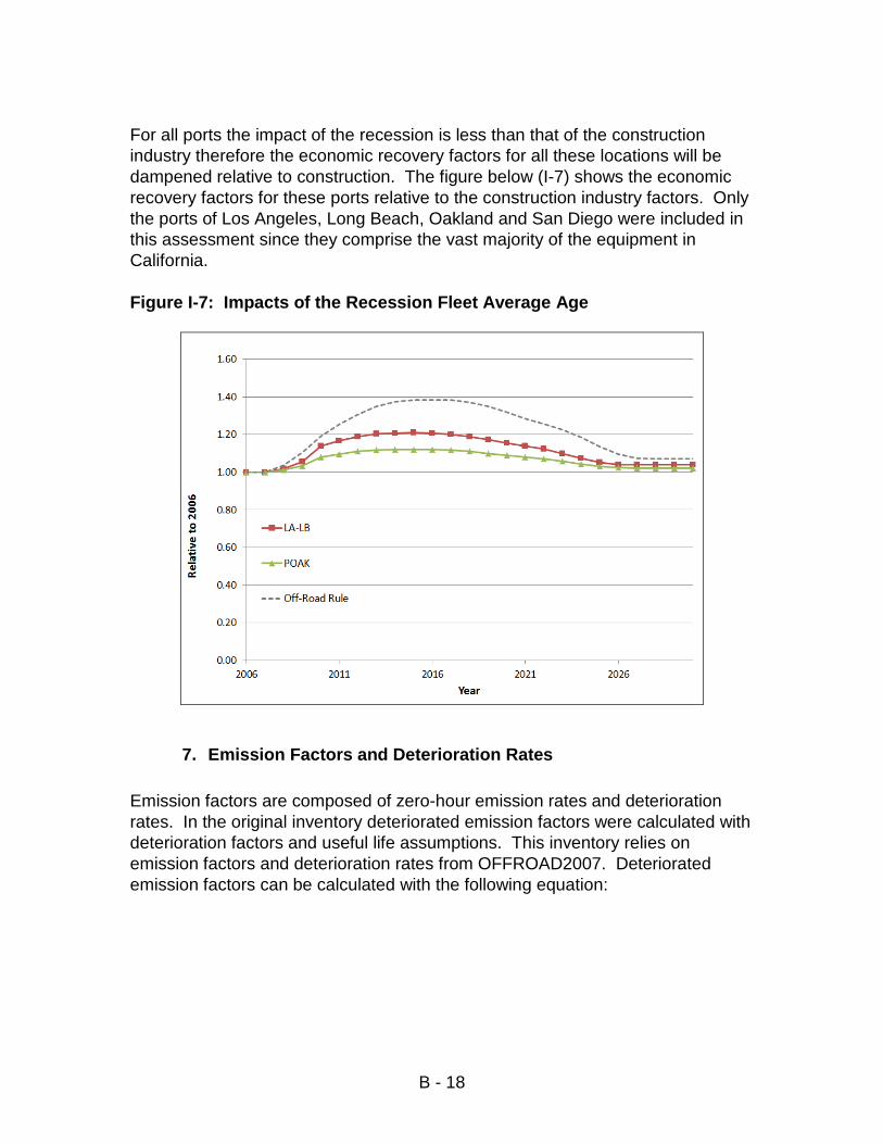
The Off-Road In-Use Equipment Regulation emissions inventory incorporated these impacts by estimating the impact of new off-road diesel equipment sales on future age distributions. Staff did this by developing economic recovery factors, which are a measure of how much a port or rail yard’s fleet ages over time. During times of economic recession, less new equipment is purchased and the average age of the fleet increases. As a result the average age of a given fleet increases comared to the base year. The economic recovery factors define the fleet average age in the future. The method, however, relies on equipment sales and economic surrogate information such as gross domestic product (GDP). (ARB, 2010b) Without equipment sales information for CHE staff relied on the same methods used for the Off-Road In-Use Equipment Regulation. (ARB, 2010b) Since construction equipment sales were proportional to GDP it was assumed the CHE sales would follow trends in TEU throughput at the ports. Staff utilized the economic recovery factors developed for the Construction and Mining Category and dampened them according to the relative difference in the impacts of the recession on the industry. For example, the Ports of Los Angeles and Long Beach (LA/LB) saw a 25% drop in TEU while the construction industry experienced nearly a 50% drop in GDP. Therefore the economic recovery factors were halved to account for this difference in recessionary impacts. This is evident in Figure I-7 which shows both the LA/LB and Off-Road recovery factors. The LA/LB factors are about half of the Off-Road factors. The Table I-9 shows the impacts of the recession for the combined ports of Los Angeles (POLA, 2010) and Long Beach (POLB, 2010), the Port of Oakland (POAK, 2010), and the Port of San Diego (AAPA, 2010): Table I-9: Impacts of the Recession on TEU

Port TEU Change 2006-2009 LA+LB 25% POAK 14% POSD 7%

B - 18

For all ports the impact of the recession is less than that of the construction industry therefore the economic recovery factors for all these locations will be dampened relative to construction. The figure below (I-7) shows the economic recovery factors for these ports relative to the construction industry factors. Only the ports of Los Angeles, Long Beach, Oakland and San Diego were included in this assessment since they comprise the vast majority of the equipment in California. Figure I-7: Impacts of the Recession Fleet Average Age

7. Emission Factors and Deterioration Rates Emission factors are composed of zero-hour emission rates and deterioration rates. In the original inventory deteriorated emission factors were calculated with deterioration factors and useful life assumptions. This inventory relies on emission factors and deterioration rates from OFFROAD2007. Deteriorated emission factors can be calculated with the following equation:

B - 19

EF = Zh + dr * CHrs Where: EF = Emission factor (g/bhp-hr) Zh = Zero-hour emission rate when the equipment is new (g/bhp-hr) Dr = Deterioration rate or the increase in zero-hour emissions as the equipment is used (g/bhp-hr2) CHrs = Cumulative hours or total number of hours accumulated on the equipment; maximum value is equal to 12,000 hours The diesel emission factors in the model are in grams per brake horsepower-hour and vary by fuel type, horsepower, and model year. To estimate fuel consumption, an emission factor is replaced with a brake-specific fuel consumption (BSFC) value (lb/hp-hr). BSFC values are used from the U.S. EPA NONROAD model. (USEPA, 2004) Emission Factors Emission factors for future years were based on the OFFROAD model which incorporates the impacts of new engine standards (Tier 3 and 4) for each year and horsepower range. The emission factors reflect any phase-in of emission standards allowed by the regulations establishing the new engine standards. Because the regulation is based on specific Tier requirements the OFFROAD2007 emission factors were updated to align with U.S. EPA horsepower bins. Deterioration rates are in units of g/hp-hr2 (grams per brake horsepower-hour-hour) and are defined as the change in emissions as a function of usage. These are based on the deterioration rates of on-highway diesel-powered engines with similar horsepower ratings. The rate of emissions changes over time as a result of wear on various parts of an engine due to use. It is assumed that at some point during the life of an equipment its engine would be rebuilt back to the standard of that particular emissions tier (varies by model year of the engine). As a result cumulative hours in the equation above is capped. In this inventory cumulative hours was capped at 12,000 hours, consistent with the Off-Road In Use Equipment Regulation, since no data was specifically available for CHE. Emission factors for on-road engines in were based on a study that tested both on-road and off-road engines in yard tractors. (ARB, 2006) The factors in Table I-10 are applied to off-road emission factors to convert them to on-road emission factors.

B - 20

Table I-10: On-Road Conversion Factors

MY HP Bin HC CO NOx PM 2003 175 0.33 1 0.44 0.70 2004 175 0.33 1 0.44 0.70 2005 175 0.33 1 0.44 0.70 2006 175 0.33 1 0.44 0.70 2007 175 0.33 1 0.69 0.70 2008 175 0.33 1 0.42 0.07 2009 175 0.33 1 0.42 0.07 2010 175 0.33 1 0.42 0.07 2011 175 0.33 1 0.07 0.07 2012 175 0.33 1 0.13 0.67 2013 175 0.33 1 0.13 0.67 2014 175 0.33 1 0.13 0.67

2015+ 175 0.33 1 0.67 0.67 2003 300 0.33 1 0.44 0.70 2004 300 0.33 1 0.44 0.70 2005 300 0.33 1 0.44 0.70 2006 300 0.33 1 0.69 0.70 2007 300 0.33 1 0.42 0.07 2008 300 0.33 1 0.42 0.07 2009 300 0.33 1 0.42 0.07 2010 300 0.33 1 0.07 0.07 2011 300 0.33 1 0.13 0.67 2012 300 0.33 1 0.13 0.67 2013 300 0.33 1 0.13 0.67

2014+ 300 0.33 1 0.67 0.67 2003 600 0.33 1 0.44 0.70 2004 600 0.33 1 0.44 0.70 2005 600 0.33 1 0.44 0.70 2006 600 0.33 1 0.69 0.70 2007 600 0.33 1 0.42 0.07 2008 600 0.33 1 0.42 0.07 2009 600 0.33 1 0.42 0.07 2010 600 0.33 1 0.07 0.07 2011 600 0.33 1 0.13 0.67 2012 600 0.33 1 0.13 0.67 2013 600 0.33 1 0.13 0.67

2014+ 600 0.33 1 0.67 0.67

B - 21

Emission Controls A number of the state’s deep-water ports have implemented cargo handling equipment emission reduction strategies using state funding, such as the Carl Moyer Program, or through port mechanisms. In addition the regulation requires the use of additional emission controls. The emissions inventory reflects the population of emission controlled equipment resulting from these programs. The reductions by emission control are consistent with the original inventory and are presented in Table I-11. These reductions are applied to the base emission rates. In some cases, such as O2 Diesel, there are emissions disbenefits. Table I-11: Emission Control Emissions Reductions (percent reduction)

Engine changes HC CO NOx PM DOC 0.7 0.7 0 0.3

DOC + O2Diesel 0.48 0.73 0.02 0.44 DPF 0 0 0 0.85

O2 Diesel -0.75 -0.1 0.02 0.2

8. Fuel Correction Factors California implemented diesel fuel regulations in 1993, which lowered the limits of aromatic compounds and the sulfur content of fuel marketed in California. The fuel correction factors (FCF) used in the emissions inventory model are dimensionless multipliers applied to the basic exhaust emission rates that account for differences in the properties of certification fuels compared to those of commercially dispensed fuels. In instances where engines or vehicles are not required to certify, the FCFs reflect the impact in changes of dispensed fuel over time as refiners respond to changes in fuel specific regulations compared to the fuel used to obtain the test data. The FCFs used in the model were specific to horsepower group and model year and were based on data described in a 2005 OFFROAD Modeling Change Technical Memo. (ARB, 2005d)

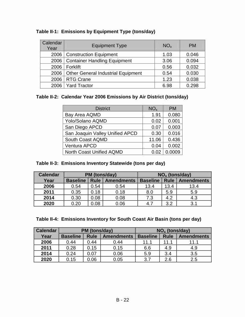
II. EMISSIONS INVENTORY RESULTS The emission inventory for cargo handling equipment includes total emissions for the locations identified in Table I-1. The data in Table II-1 summarizes the statewide inventory of oxides of nitrogen (NOx) and diesel particulate matter (PM) for 2006 by equipment type. Combined yard trucks, container handling equipment (top picks, sides picks, etc.), and cranes are responsible for approximately 85 percent of the emissions for all pollutants.

B - 22

Table II-1: Emissions by Equipment Type (tons/day)

Calendar Year Equipment Type NOx PM

2006 Construction Equipment 1.03 0.046 2006 Container Handling Equipment 3.06 0.094 2006 Forklift 0.56 0.032 2006 Other General Industrial Equipment 0.54 0.030 2006 RTG Crane 1.23 0.038 2006 Yard Tractor 6.98 0.298

Table II-2: Calendar Year 2006 Emissions by Air District (tons/day)

District NOx PM Bay Area AQMD 1.91 0.080 Yolo/Solano AQMD 0.02 0.001 San Diego APCD 0.07 0.003 San Joaquin Valley Unified APCD 0.30 0.016 South Coast AQMD 11.06 0.436 Ventura APCD 0.04 0.002 North Coast Unified AQMD 0.02 0.0009

Table II-3: Emissions Inventory Statewide (tons per day) Calendar

Year PM (tons/day) NOx (tons/day)

Baseline Rule Amendments Baseline Rule Amendments 2006 0.54 0.54 0.54 13.4 13.4 13.4 2011 0.35 0.18 0.18 8.0 5.9 5.9 2014 0.30 0.08 0.08 7.3 4.2 4.3 2020 0.20 0.08 0.06 4.7 3.2 3.1

Table II-4: Emissions Inventory for South Coast Air Basin (tons per day) Calendar

Year PM (tons/day) NOx (tons/day)

Baseline Rule Amendments Baseline Rule Amendments 2006 0.44 0.44 0.44 11.1 11.1 11.1 2011 0.28 0.15 0.15 6.6 4.9 4.9 2014 0.24 0.07 0.06 5.9 3.4 3.5 2020 0.15 0.06 0.05 3.7 2.6 2.5

B - 23

Table II-5: Emissions Inventory for San Francisco Air Basin (tons per day) Calendar

Year PM (tons/day) NOx (tons/day)

Baseline Rule Amendments Baseline Rule Amendments 2006 0.08 0.08 0.08 1.9 1.9 1.9 2011 0.05 0.03 0.03 1.1 0.9 0.9 2014 0.05 0.01 0.01 1.1 0.7 0.7 2020 0.03 0.01 0.01 0.8 0.5 0.5

B - 24

III. References (ARB, 2011f) California Air Resources Board, “Cargo Handling Emissions Inventory Model,” July 2011. http://www.arb.ca.gov/ports/cargo/cheamd2011.htm (ARB, 2011o) California Air Resources Board, “Cargo Handling Emissions Inventory Model Working Files,” July 2011. http://www.arb.ca.gov/ports/cargo/cheamd2011.htm

(ARB, 2005b) California Air Resources Board, CHE Survey, 2005. (USEPA, 2005) U.S. Environmental Protection Agency, Calculation of Age Distributions in the Nonroad Model: Growth and Scrappage, 2005. http://nepis.epa.gov/Adobe/PDF/P1004L8U.PDF (ARB, 2005c) California Air Resources Board, CHE Equipment 2005 Reporting Data, 2005. (Starcrest, 2010a) Starcrest Consulting, Port of Los Angeles Inventory of Air Emissions 2009, June 2010. http://www.portoflosangeles.org/environment/studies_reports.asp (Starcrest, 2010b) Starcrest Consulting, Port of Long Beach Air Emissions Inventory, June 2010. http://www.polb.com/environment/air/emissions.asp (Environ, 2008) Environ International Corporation, Port of Oakland 2005 Seaport Air Emissions Inventory, March 2008. http://www.portofoakland.com/environm/airEmissions.asp (ARB, 2008) California Air Resources Board, Railyard Health Risk Assessments and Mitigation Measures, 2008. http://www.arb.ca.gov/railyard/hra/hra.htm (Starcrest, 2008a) Starcrest Consulting, Port of Los Angeles 2006 Emissions Inventory, July 2008. http://www.portoflosangeles.org/DOC/REPORT_Air_Emissions_Inventory_Volume1.pdf (Starcrest, 2008b) Starcrest Consulting, Port of Long Beach Emissions Inventory 2006, June 2008. http://www.polb.com/environment/air/emissions.asp

B - 25

(Starcrest, 2008c) Starcrest Consulting, The Port of San Diego 2006 Emissions Inventory, March 2008. http://www.portofsandiego.org/environment/clean-air.html#doc (ARB, 2007) California Air Resources Board, OFFROAD2007 Model, 2007. http://www.arb.ca.gov/msei/offroad/offroad.htm (ARB, 2011l) California Air Resources Board, Appendix D: Emissions Estimation Methodology for Ocean-Going Vessels, 2011. http://www.arb.ca.gov/regact/2011/ogv11/ogv11appd.pdf (ARB, 2010b) California Air Resources Board, APPENDIX D: OSM AND SUMMARY OF OFF-ROAD EMISSIONS INVENTORY UPDATE, 2010. http://www.arb.ca.gov/regact/2010/offroadlsi10/offroadappd.pdf (ARB, 2010c) California Air Resources Board, Preliminary Results of Joint ARB/DOSH/OSHSB Field Study of Retrofit Feasibility for Most Common Vehicles, May 2010. (POLA, 2010) Port of Los Angeles, Port of Los Angeles Container Statistics – 2010, 2010. http://www.portoflosangeles.org/maritime/stats_2010.asp (POLB, 2010) Port of Long Beach, Port of Long Beach Container Statistics – 2010, 2010. http://www.polb.com/economics/stats/yearly_teus.asp (POAK, 2010) Port of Oakland, Container History - Port of Oakland TEU's Activity (1990 - 2010), 2010. http://www.portofoakland.com/maritime/facts_cargo.asp (AAPA, 2010) American Association of Port Authorities, North America: Container Port Traffic 1990-2010, 2011. http://www.aapa-ports.org/industry/content.cfm?ItemNumber=900&navItemNumber=551 (USEPA, 2004) U.S. Environmental Protection Agency, NONROAD Model (nonroad engines, equipment, and vehicles), 2004. http://www.epa.gov/oms/nonrdmdl.htm (ARB, 2006) California Air Resources Board, Cargo Handling Equipment Yard Truck Emission Testing, 2006. http://www.arb.ca.gov/ports/cargo/documents/yttest.pdf

B - 26

(ARB, 2005d) California Air Resources Board, OFFROAD Modeling Change Technical Memo, OFF-ROAD EXHAUST EMISSIONS INVENTORY FUEL CORRECTION FACTORS, 2005. http://www.arb.ca.gov/msei/offroad/techmemo/arb_offroad_fuels.pdf

B - 27

Appendix A

Categorization of Similar Equipment Equipment Category Location

Construction Equipment H Port of Humboldt Bay Construction Equipment H Port of Richmond Construction Equipment H Port of Stockton Construction Equipment H UPRR Oakland Construction Equipment L BNSF Stockton Construction Equipment L Other Bay Area Ports & Railyards Construction Equipment L Port of Long Beach Construction Equipment L Port of Redwood City Construction Equipment L Port of Sacramento Construction Equipment L Port of San Francisco Construction Equipment L San Diego Port & Railyard Construction Equipment M Port of Los Angeles Construction Equipment M Port of Oakland Container Handling Equipment H BNSF Fresno Container Handling Equipment H BNSF Los Angeles Container Handling Equipment H BNSF Oakland Container Handling Equipment H BNSF San Bernardino Container Handling Equipment H Port of Hueneme Container Handling Equipment H Port of San Francisco Container Handling Equipment H Port of Stockton Container Handling Equipment H San Diego Port & Railyard Container Handling Equipment H UPRR City of Industry Container Handling Equipment H UPRR ICTF Container Handling Equipment H UPRR LA/Commerce Container Handling Equipment H UPRR LATC Container Handling Equipment H UPRR Lathrop Container Handling Equipment L BNSF Stockton Container Handling Equipment L Port of Long Beach Container Handling Equipment L Port of Los Angeles Container Handling Equipment L Port of Oakland Container Handling Equipment L UPRR Oakland Forklift H Port of Hueneme Forklift H Port of Oakland Forklift H Port of Sacramento Forklift H UPRR LA/Commerce Forklift L BNSF Fresno Forklift L BNSF Oakland

B - 28

Categorization of Similar Equipment Equipment Category Location

Forklift L BNSF San Bernardino Forklift L BNSF Stockton Forklift L Other Bay Area Ports & Railyards Forklift L Port of Redwood City Forklift L UPRR City of Industry Forklift L UPRR ICTF Forklift L UPRR LATC Forklift L UPRR Lathrop Forklift L UPRR Oakland Forklift M BNSF Los Angeles Forklift M Port of Long Beach Forklift M Port of Los Angeles Forklift M Port of Stockton Forklift O Port of Humboldt Bay Forklift O Port of Richmond Forklift O Port of San Francisco Forklift O San Diego Port & Railyard Other General Industrial Equipment H BNSF Los Angeles Other General Industrial Equipment H Port of Hueneme Other General Industrial Equipment H Port of Long Beach Other General Industrial Equipment H Port of Oakland Other General Industrial Equipment H Port of Redwood City Other General Industrial Equipment H Port of Richmond Other General Industrial Equipment H Port of Sacramento Other General Industrial Equipment H Port of Stockton Other General Industrial Equipment H UPRR ICTF Other General Industrial Equipment H UPRR Lathrop Other General Industrial Equipment H UPRR Oakland Other General Industrial Equipment L BNSF Stockton Other General Industrial Equipment L Port of Los Angeles Other General Industrial Equipment L San Diego Port & Railyard Other General Industrial Equipment L UPRR LA/Commerce RTG Crane H BNSF Fresno RTG Crane H BNSF Richmond RTG Crane H Other Bay Area Ports & Railyards RTG Crane H Port of Hueneme RTG Crane H Port of Oakland RTG Crane H UPRR City of Industry RTG Crane H UPRR LA/Commerce RTG Crane L BNSF Commerce

B - 29

Categorization of Similar Equipment Equipment Category Location

RTG Crane L BNSF Los Angeles RTG Crane L BNSF San Bernardino RTG Crane L BNSF Stockton RTG Crane L Port of Long Beach RTG Crane L Port of Los Angeles RTG Crane L UPRR ICTF RTG Crane L UPRR LATC RTG Crane L UPRR Lathrop RTG Crane L UPRR Oakland Yard Tractor H BNSF Fresno Yard Tractor H BNSF Oakland Yard Tractor H BNSF Richmond Yard Tractor H BNSF San Bernardino Yard Tractor H Other Bay Area Ports & Railyards Yard Tractor H Port of Hueneme Yard Tractor H Port of Humboldt Bay Yard Tractor H Port of Long Beach Yard Tractor H Port of Los Angeles Yard Tractor H Port of Oakland Yard Tractor H Port of Redwood City Yard Tractor H Port of Sacramento Yard Tractor H Port of San Francisco Yard Tractor H Port of Stockton Yard Tractor H San Diego Port & Railyard Yard Tractor H UPRR LA/Commerce Yard Tractor L BNSF Commerce Yard Tractor L BNSF Los Angeles Yard Tractor L BNSF Stockton Yard Tractor L UPRR City of Industry Yard Tractor L UPRR ICTF Yard Tractor L UPRR LATC Yard Tractor L UPRR Lathrop Yard Tractor L UPRR Oakland

B - 30

Appendix B Growth Rates:

Area Year Growth Factor Bay Area 2000 0.73 Bay Area 2001 0.77 Bay Area 2002 0.82 Bay Area 2003 0.86 Bay Area 2004 0.90 Bay Area 2005 0.95 Bay Area 2006 1.00 Bay Area 2007 0.89 Bay Area 2008 0.84 Bay Area 2009 0.66 Bay Area 2010 0.70 Bay Area 2011 0.76 Bay Area 2012 0.81 Bay Area 2013 0.88 Bay Area 2014 0.96 Bay Area 2015 1.04 Bay Area 2016 1.11 Bay Area 2017 1.20 Bay Area 2018 1.26 Bay Area 2019 1.32 Bay Area 2020 1.36 Bay Area 2021 1.42 Bay Area 2022 1.47 Bay Area 2023 1.53 Bay Area 2024 1.59 Bay Area 2025 1.67 Bay Area 2026 1.73 Bay Area 2027 1.80 Bay Area 2028 1.82 Bay Area 2029 1.83 Bay Area 2030 1.82 Port Hueneme 2000 0.99 Port Hueneme 2001 0.99 Port Hueneme 2002 0.99 Port Hueneme 2003 0.99 Port Hueneme 2004 1.00 Port Hueneme 2005 1.00 Port Hueneme 2006 1.00

B - 31

Port Hueneme 2007 0.87 Port Hueneme 2008 0.80 Port Hueneme 2009 0.61 Port Hueneme 2010 0.63 Port Hueneme 2011 0.66 Port Hueneme 2012 0.69 Port Hueneme 2013 0.73 Port Hueneme 2014 0.77 Port Hueneme 2015 0.82 Port Hueneme 2016 0.85 Port Hueneme 2017 0.89 Port Hueneme 2018 0.91 Port Hueneme 2019 0.93 Port Hueneme 2020 0.94 Port Hueneme 2021 0.95 Port Hueneme 2022 0.96 Port Hueneme 2023 0.97 Port Hueneme 2024 0.99 Port Hueneme 2025 1.00 Port Hueneme 2026 1.02 Port Hueneme 2027 1.03 Port Hueneme 2028 1.05 Port Hueneme 2029 1.07 Port Hueneme 2030 1.08 San Diego 2000 1.05 San Diego 2001 1.04 San Diego 2002 1.03 San Diego 2003 1.02 San Diego 2004 1.02 San Diego 2005 1.01 San Diego 2006 1.00 San Diego 2007 0.90 San Diego 2008 0.86 San Diego 2009 0.69 San Diego 2010 0.74 San Diego 2011 0.81 San Diego 2012 0.88 San Diego 2013 0.97 San Diego 2014 1.07 San Diego 2015 1.18 San Diego 2016 1.29

B - 32

San Diego 2017 1.41 San Diego 2018 1.50 San Diego 2019 1.60 San Diego 2020 1.68 San Diego 2021 1.78 San Diego 2022 1.88 San Diego 2023 1.99 San Diego 2024 2.11 San Diego 2025 2.25 San Diego 2026 2.38 San Diego 2027 2.52 San Diego 2028 2.69 San Diego 2029 2.87 San Diego 2030 3.04 South Coast 2000 0.73 South Coast 2001 0.77 South Coast 2002 0.81 South Coast 2003 0.86 South Coast 2004 0.90 South Coast 2005 0.95 South Coast 2006 1.00 South Coast 2007 0.91 South Coast 2008 0.88 South Coast 2009 0.71 South Coast 2010 0.77 South Coast 2011 0.84 South Coast 2012 0.92 South Coast 2013 1.03 South Coast 2014 1.13 South Coast 2015 1.26 South Coast 2016 1.38 South Coast 2017 1.52 South Coast 2018 1.63 South Coast 2019 1.75 South Coast 2020 1.85 South Coast 2021 1.97 South Coast 2022 2.09 South Coast 2023 2.22 South Coast 2024 2.37 South Coast 2025 2.53 South Coast 2026 2.69

B - 33

South Coast 2027 2.86 South Coast 2028 3.06 South Coast 2029 3.27 South Coast 2030 3.48

B - 34

THIS PAGE INTENTIONALLY LEFT BLANK