Appendix A Tookany/Tacony-Frankford Creek SWMM Validation
151
Appendix A Tookany/Tacony-Frankford Creek SWMM Validation
Transcript of Appendix A Tookany/Tacony-Frankford Creek SWMM Validation
Appendix A
Tookany/Tacony-Frankford Creek SWMM Validation

Appendix A: Tookany/Tacony-Frankford Creek SWMM Validation Page A-2 Philadelphia Water Department June 2013
A.1 Introduction This appendix describes the development and validation of the Tookany/Tacony-Frankford Creek Tributary H&H Model used to provide the hydraulic and bacteria loadings to the United States Environmental Protection Agency (US EPA) Water Quality Analysis Simulation Program (WASP) model.
The US EPA Storm Water Management Model (SWMM) version 5 was used to develop the Combined Sewer System (CSS) Model and Watershed Model that comprise the Tributary Hydraulic and Hydrologic (H&H) Model. SWMM hydrology, represented by subcatchments, simulated both the quantity and quality of runoff in a drainage basin and the routing of flows and contaminants to sewers or receiving waters. SWMM hydrology can accept precipitation (rainfall or snowfall) hyetographs and perform a step by step accounting of snowmelt, infiltration losses in pervious areas, surface detention, overland flow, and water quality constituents leading to the calculation of one or more hydrographs and/or pollutographs at a certain geographic point such as a sewer inlet. SWMM hydraulics, represented by nodes and links, simulate dynamic hydraulic flow routing and pollutant routing through open channel and closed conduit systems (US EPA, 2010).
The Tookany/Tacony-Frankford Creek Tributary H&H Model was developed to simulate the stormwater runoff and water quality loading from combined sewer overflows (CSOs) and minor tributaries to the receiving waters. The model was developed primarily utilizing information obtained through previous modeling efforts and Geographic Information Systems (GIS), and was driven using continuous radar rainfall time series. Event mean concentrations (EMCs) were used to predict the stormwater quality components of the model. Flow validations were performed using monitoring records from United States Geological Survey (USGS) gaging stations. The model validation period of the Tributary H&H Model was dictated by available USGS streamflow and radar rainfall data.
The following sections of this report further describe the models used in development and validation of the Tookany/Tacony-Frankford Creek Tributary H&H Model.
A.2 Discussion of Legacy Models and Reports Several previously published models and reports were used to develop the Tookany/Tacony-Frankford Creek Tributary H&H Model. This section discusses the role of legacy publications in model development.
A.2.1 Long Term Control Plan Update Combined Sewer System (CSS) Model The Northeast District combined sewer system of Philadelphia was originally modeled as part of the Long Term Control Plan (Philadelphia Water Department, 1997). Additional refinement of the CSS Model occurred as part of the Long Term Control Plan Update. Combined sewer system

Appendix A: Tookany/Tacony-Frankford Creek SWMM Validation Page A-3 Philadelphia Water Department June 2013
model development and calibration methodology are discussed within Supplemental Documentation Volume 4 (Philadelphia Water Department, 2011).
The CSS Model domain included:
• The combined service area within the City borders, which drains to the Philadelphia Water Department (Water Department) Water Pollution Control Plants.
• The sanitary portion of the separate sewered area, within and outside the City, which drains to the Water Department Water Pollution Control Plants. A simplified version of the sanitary collection system is modeled inside the City, and indirectly modeled outside the City.
• The combined sewer overflow and interceptor relief outfall pipes within the City, which discharge into the receiving waters.
A.2.2 HEC-2 Model An open channel HEC-2 model of Tookany/Tacony-Frankford Creek was developed as part of a Federal Emergency Management Agency (FEMA) Flood Insurance Study (FIS). The Tookany/Tacony-Frankford Creek HEC-2 Model was originally developed in 1974 (Federal Emergency Management Agency, 2001). Channel geometry data within the Tookany/Tacony-Frankford Creek Watershed Model was supplemented with historic FEMA HEC-2 model data.
A.2.3 Fluvial Geomorphology (FGM) Study Fluvial geomorphology data was collected as part of the Tookany/Tacony-Frankford Creek Watershed Comprehensive Characterization Report (Philadelphia Water Department, 2005). Channel geometry and bed roughness data derived in the FGM study were used in development of the Tookany/Tacony-Frankford Creek Watershed Model.
A.2.4 Act 167 Stormwater Management Plan A coupled CSS and Watershed Model of Tookany/Tacony-Frankford Creek was developed as part of the Tookany/Tacony-Frankford Creek Act 167 Stormwater Management Plan (Philadelphia Water Department, 2008). The Northeast District CSS Model was integrated into a model of the Tookany/Tacony-Frankford Creek watershed. Outfall pipes from the regulator structures in the CSS Model were connected to open channel nodes of the Watershed Model so wet weather overflows could be routed to the Tookany/Tacony-Frankford Creek. The result was a model that included the collection system pipe network and all upstream inputs. The model developed for the Act 167 Plan served as the starting point for Tributary H&H Model development.
The Act167 Model domain included:
• The combined service area within the City borders, which drains to the Water Department Water Pollution Control Plants.
• The sanitary portion of the separate sewered area, within and outside the City, which drains to the Water Department Water Pollution Control Plants. A simplified version

Appendix A: Tookany/Tacony-Frankford Creek SWMM Validation Page A-4 Philadelphia Water Department June 2013
of the sanitary collection system is modeled inside the City, and indirectly modeled outside the City.
• The combined sewer overflow and interceptor relief outfall pipes within the City, which discharge into receiving waters.
• Open channel representations of the receiving waters and major tributaries within the watershed.
• The stormwater and direct runoff areas within and outside of the City borders. Stormwater collection system conduits are not explicitly modeled.
A.3 Model Development The coupled CSS and Watershed Model of Tookany/Tacony-Frankford Creek, developed as part of the Tookany/Tacony-Frankford Creek Act 167 Plan report, served as the starting point for Tributary H&H Model development. The Act 167 Model was simplified by removing bridges, short culverts, and short cross sections. This simplification also improved model stability. The simplified model is referred to as the Tributary H&H Model and was validated against two USGS stream gages. This model provides the hydraulic and bacteria loadings to the WASP model.
The Tookany/Tacony-Frankford Creek Tributary H&H Model includes the entire stream drainage area and extends beyond the Water Department service area into Montgomery County. The model representation of both the channel and the watershed areas beyond the Water Department service area was intended to capture the water quality effect of outfall T-01 which discharges to Rock Creek, a small tributary stream upstream of the City boundary. Figure 1-5 shows the model extents, subwatershed areas, and locations of Water Department and municipal collection system CSOs within the watershed area. In addition to the main channel of Tookany/Tacony-Frankford Creek, several smaller streams were represented in the model to control and improve the timing and shape of the simulated hydrograph at the validation locations.
Within the City, both combined sewer and sanitary sewered areas are included in the Tributary H&H Model. Watershed areas outside the City and outside the CSS are also accounted for in the model. The non-combined sewer areas are mostly within the communities neighboring the City of Philadelphia to the north and west. These areas contribute runoff and associated pollutant loads to the receiving waters either through stormwater collection systems, direct runoff, or through minor tributary waterways.
A.3.1 Hydraulic Model Development SWMM uses a link-node description of sewer and open channel systems facilitating the physical prototype and the mathematical solution of the gradually-varied unsteady flow (St. Venant) equations which form the mathematical basis of the model. The links transmit the flow from node to node. Properties associated with the links include roughness, length, cross-sectional area, hydraulic radius, and surface width. The primary dependent variable for the links is discharge. Variables associated with nodes include volume, head, and surface area. The
Appendix A: Tookany/Tacony-Frankford Creek SWMM Validation Page A-5 Philadelphia Water Department June 2013
primary dependent variable for nodes is head, which is assumed to be changing in time, but constant throughout any one node.
Open Chanel Cross Sections The hydraulic network consisted of open channel representations of the Tookany/Tacony-Frankford Creek and major tributaries within the watershed. It was developed from two separate data sets:
• Cross sectional data from HEC-2 models used in the Philadelphia County FIS
• Cross sectional data obtained through the FGM Study
The Water Department surveyed cross sections were used as the main channel for the Tookany/Tacony-Frankford Creek Act 167 Model; the Act 167 Model was the starting point for development of the open channel portion of the Tributary H&H Model. For the Act 167 Model , the cross sections were extended by using GIS data to draw lines perpendicular to 2 ft contour lines. The extended cross sections were then plotted in MS Excel and corrected if any obvious elevation discontinuities existed between the two data sets. Because contour lines are taken to a datum, the surveyed cross section was shifted up or down to be a smooth extension of the contours. Cross sections were extended until they reached about 40 ft higher than the stream bed elevation and were assumed to be representative until the next upstream survey point. Cross sections were also drawn for the top decks of bridges and culverts using the 2 ft contours to accurately model flood conditions in the Act 167 Plan. However, these bridges and short culverts were removed to improve model stability in the Tributary H&H model.
The Water Department stream survey ended roughly at Bristol Street. Between this point and the Delaware River, data from the Philadelphia County FIS HEC-2 Model of the Tookany/Tacony-Frankford Creek was used to supplement the stream survey. Where the two data sets overlapped, cross sections were compared. The two models agreed fairly well so it was assumed HEC-2 cross sections, while less accurate, were a reasonable approximation. All Water Department surveyed cross sections along the main stem of the Tookany/Tacony-Frankford Creek were sorted by river mile and connected.
Minor tributaries were assembled individually and tied into the main stem. Because the Water Department surveys did not exist at the exact location where tributaries tie into the mainstem, the elevation of these points were interpolated from the Water Department cross sections on either side.
The resultant tributary channel network consisted of over 200 channel cross sections representing more than 22 miles of stream. Since conduit length is the primary constraint when stabilizing a model, some conduits were replaced with lengthened equivalent conduits before being put into the model. However, this was done only when necessary. The Act 167 Model contains documentation of extended reaches. In the Tookany/Tacony-Frankford Creek Tributary H&H Model, bridge crossings, most culverts, and short channels were consolidated and simplified to longer open channel conduits. The hydraulic configurations of the stream are based upon the best available information, but should not be considered a truly accurate depiction of actual stream conditions beyond the objectives of the water quality modeling tasks.
Appendix A: Tookany/Tacony-Frankford Creek SWMM Validation Page A-6 Philadelphia Water Department June 2013
All elevations within the model are based on inverts calculated from the topographic contours and surveyed cross sections. Ground elevations are set as the maximum elevation found in the station elevation pairs defining any natural cross section. They are sufficiently high to prevent the hydraulic grade line within the channel from exceeding the user defined channel elevation.
The Water Department pebble counts along Tookany/Tacony-Frankford Creek were used to estimate the value for Manning’s roughness within the channel. Channel roughness values for the Tookany/Tacony-Frankford Creek were assigned at all Water Department channel survey points. These roughness values are assumed to be representative until the next upstream survey point.
Floodplain roughness values for the transects were estimated from ortho-photography, field photographs at all Water Department survey points, and a flyover video of Frankford Creek. These values are assumed to be representative until the next upstream survey point.
A.3.2 Hydrologic Model Development Subcatchment Delineation Watersheds were delineated for the Tookany/Tacony-Frankford Creek using GIS surface contour layers obtained from Pennsylvania Spatial Data Access (PASDA). Sheds were delineated to survey rebars and were defined by 2 ft topographic contour lines. Subcatchment watersheds were delineated to selected points along the main channel at critical stream junctions or at pre-defined intervals. Since runoff from combined areas reaches the receiving water as a CSO input, sheds were defined for any watershed area not defined as a CSO subcatchment in the CSS Model. In this way runoff from areas defined as sanitary service areas, storm sheds, and non-contributing areas (to the collection system) was included in the Watershed Model. The defined subwatersheds serve as the modeling unit in the Tributary H&H Model.
Overland Slope In SWMM, runoff is calculated by approximating a non-linear reservoir which forms above the surface once the demands of infiltration, evaporation, and storage have been satisfied. The overland flow is generated using Manning’s equation:
Where: Q = surface runoff (cfs), W = width of watershed (ft), S = average slope of watershed (ft/ft) d = depth in the non-linear reservoir (ft), n = Manning roughness coefficient, and ds = depression storage depth in the non-linear reservoir (ft).
Overland slope is a quantifiable physical parameter and is not adjusted during model validation. An average overland flow slope technique was used to define subcatchment slopes for the Tookany/Tacony-Frankford Creek Tributary H&H Model.
Appendix A: Tookany/Tacony-Frankford Creek SWMM Validation Page A-7 Philadelphia Water Department June 2013
The average slope values of the Tookany/Tacony-Frankford sheds were found by using Spatial Analyst, a toolset in ArcGIS that analyzes and models cell based data. The average slope was calculated by using a 1 arc-second DEM that was bounded by a polygon feature class representation of the model subcatchments. Within Spatial Analyst, the "Slope" function calculates the maximum rate of change in value from that cell to its neighbors. For this analysis, the percent slope was calculated and redrawn as a new raster file. The "Zonal Statistics" function was then used to average the slope values within the shed boundaries.
Width The width parameter impacts the time of concentration and the hydrograph shape in the hydrologic portion of SWMM. Subcatchments are represented as rectangular areas defined by the subcatchment width parameter. By definition, the width of a watershed is equal to the area of the watershed divided by the length of the overland flow path. The width parameter is one of the main validation parameters used to adjust hydrograph shape, and to some degree hydrograph volume. Watersheds assigned a large width, and therefore a small overland flow length, will have a short time of concentration. Reducing width increases the flow length and will thus increase the time of concentration. Increasing the overland flow length also reduces the runoff volume as the flow is exposed to evaporation and infiltration over pervious areas for a longer period of time. Stormwater collection systems and minor undefined waterways are examples of how the overland flow length can be shortened, and the width increased. Overland flow length is a more intuitive parameter, and therefore is used as the basis for adjusting and discussing the SWMM width parameter. Since the width parameter is adjusted during validation, it is only necessary to obtain an approximate initial value.
The initial estimates for watershed width were obtained by calculating two times the square root of the watershed area. This approach provides a width based on an idealized square watershed along the middle of the watershed. Since actual watersheds are not rectangular with properties of symmetry and uniformity, it should be expected that these values will be widely adjusted during the validation process.
Gross Impervious Cover An estimate of gross impervious area for model subcatchments was based on clipping the Water Department impervious surface coverage with the Tookany/Tacony-Frankford Creek subcatchment shed coverage and calculating the percent impervious cover for each subcatchment. Impervious surface information was obtained from the 2004 Sanborn planimetric layer maintained by the Office of Watersheds. Impervious surface classifications in the layer were grouped into three broad categories (buildings, parking, streets/sidewalks). For each subcatchment, the area of impervious surface was summed to generate a total impervious area.
Land use data was used to estimate impervious cover for portions of the watershed areas outside of the Water Department service area and within neighboring Montgomery County. The Delaware Valley Regional Planning Commission completed a digital land use file based on aerial photography flown in March through May of 1995 that was used in this analysis. Land use was interpreted in seventeen categories from 1330 Photo Atlas Sheets at the 1 inch = 400 ft. scale.
Appendix A: Tookany/Tacony-Frankford Creek SWMM Validation Page A-8 Philadelphia Water Department June 2013
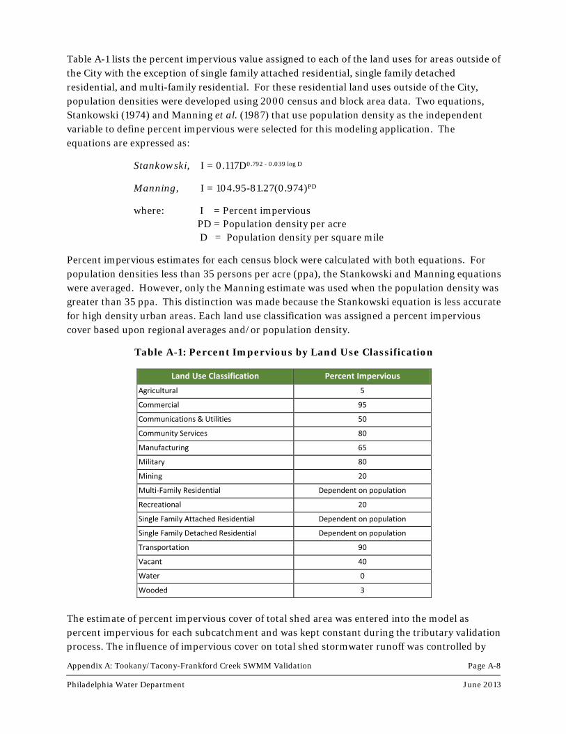
Table A-1 lists the percent impervious value assigned to each of the land uses for areas outside of the City with the exception of single family attached residential, single family detached residential, and multi-family residential. For these residential land uses outside of the City, population densities were developed using 2000 census and block area data. Two equations, Stankowski (1974) and Manning et al. (1987) that use population density as the independent variable to define percent impervious were selected for this modeling application. The equations are expressed as:
Stankowski, I = 0.117D0.792 - 0.039 log D
Manning, I = 104.95-81.27(0.974)PD
where: I = Percent impervious PD = Population density per acre D = Population density per square mile
Percent impervious estimates for each census block were calculated with both equations. For population densities less than 35 persons per acre (ppa), the Stankowski and Manning equations were averaged. However, only the Manning estimate was used when the population density was greater than 35 ppa. This distinction was made because the Stankowski equation is less accurate for high density urban areas. Each land use classification was assigned a percent impervious cover based upon regional averages and/or population density.
Table A-1: Percent Impervious by Land Use Classification
Land Use Classification Percent Impervious Agricultural 5
Commercial 95
Communications & Utilities 50
Community Services 80
Manufacturing 65
Military 80
Mining 20
Multi-Family Residential Dependent on population
Recreational 20
Single Family Attached Residential Dependent on population
Single Family Detached Residential Dependent on population
Transportation 90
Vacant 40
Water 0
Wooded 3
The estimate of percent impervious cover of total shed area was entered into the model as percent impervious for each subcatchment and was kept constant during the tributary validation process. The influence of impervious cover on total shed stormwater runoff was controlled by

Appendix A: Tookany/Tacony-Frankford Creek SWMM Validation Page A-9 Philadelphia Water Department June 2013
the percent routed parameter, which was considered to be the impervious runoff validation parameter.
Percent Impervious Cover Routed SWMM simulates surface runoff from drainage areas using three “planes” of overland flow. One plane represents all impervious surfaces directly connected to the hydraulic system and included initial abstraction or surface detention storage (puddles, cracks, etc. which do not permit immediate runoff). A second plane represents all pervious areas and impervious areas not directly connected to the hydraulic system. The third plane is defined as the fraction of the directly connected area that provides no detention storage and thus produces runoff immediately. Furthermore, a portion of the pervious runoff can be routed to the impervious surface (i.e. Pervious Routing), or a portion of the impervious runoff can be routed to the pervious surface (i.e. Impervious Routing). The runoff from the drainage area is the sum of the flow from the three planes, after considering internal routing.
Impervious surfaces, by definition, do not have an infiltration component. However, impervious surfaces are not always connected to a collection or conveyance system, and may instead route to a pervious surface where the runoff generated has the opportunity to infiltrate. The fraction of the total area that is impervious and drains directly to the collection or conveyance system is defined as the directly connected impervious area (DCIA). In SWMM, the “% Impervious” hydrologic parameter represents the gross impervious area as a percentage of the total shed area. The PERVIOUS method of subcatchment routing is used to approximate hydrograph flow paths from the subcatchments. When the PERVIOUS method is used, a value for the percent of total runoff from the impervious area that is routed over the remaining pervious area of the shed is defined. The remaining impervious area not routed is termed the DCIA, which drains directly to the collection and conveyance system. The PERVIOUS routing method allows for complex hydrographs to be reproduced as DCIA is manifested as a near immediate system response to precipitation, while the pervious area runoff may have a slower response.
Soils The rate of infiltration is a function of soil properties in the drainage area, ground slopes, and ground cover. The Green-Ampt method of calculating infiltration was employed for the Tookany/Tacony-Frankford Creek Tributary H&H Model. The Green-Ampt equation for infiltration has physically based parameters that can be estimated based on soil characteristics. The soil parameters used in this method are: average capillary suction, saturated hydraulic conductivity, and the initial moisture deficit. In SWMM, pervious area runoff is generated when rainfall volume and intensity exceed the soil infiltration capacity and evaporation demands. Infiltration is primarily controlled by setting the soil saturated hydraulic conductivity, which is the rate at which water will infiltrate the soil after the soil has reached a point of saturation. By lowering the saturated hydraulic conductivity, the pervious area begins to generate runoff. Once the saturated hydraulic conductivity threshold for pervious runoff is found, additional increment adjustments downward tend to produce very significant responses. Therefore, saturated hydraulic conductivity was a primary validation parameter.
Soil information for the Tookany/Tacony-Frankford Creek watershed was obtained from the
Appendix A: Tookany/Tacony-Frankford Creek SWMM Validation Page A-10 Philadelphia Water Department June 2013
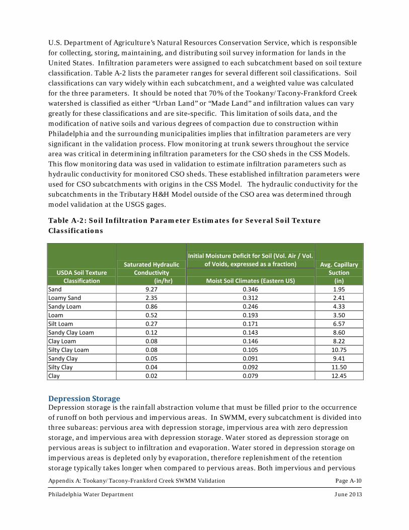
U.S. Department of Agriculture’s Natural Resources Conservation Service, which is responsible for collecting, storing, maintaining, and distributing soil survey information for lands in the United States. Infiltration parameters were assigned to each subcatchment based on soil texture classification. Table A-2 lists the parameter ranges for several different soil classifications. Soil classifications can vary widely within each subcatchment, and a weighted value was calculated for the three parameters. It should be noted that 70% of the Tookany/Tacony-Frankford Creek watershed is classified as either “Urban Land” or “Made Land” and infiltration values can vary greatly for these classifications and are site-specific. This limitation of soils data, and the modification of native soils and various degrees of compaction due to construction within Philadelphia and the surrounding municipalities implies that infiltration parameters are very significant in the validation process. Flow monitoring at trunk sewers throughout the service area was critical in determining infiltration parameters for the CSO sheds in the CSS Models. This flow monitoring data was used in validation to estimate infiltration parameters such as hydraulic conductivity for monitored CSO sheds. These established infiltration parameters were used for CSO subcatchments with origins in the CSS Model. The hydraulic conductivity for the subcatchments in the Tributary H&H Model outside of the CSO area was determined through model validation at the USGS gages.
Table A-2: Soil Infiltration Parameter Estimates for Several Soil Texture Classifications
USDA Soil Texture Classification
Saturated Hydraulic Conductivity
(in/hr)
Initial Moisture Deficit for Soil (Vol. Air / Vol. of Voids, expressed as a fraction) Avg. Capillary
Suction (in) Moist Soil Climates (Eastern US)
Sand 9.27 0.346 1.95 Loamy Sand 2.35 0.312 2.41 Sandy Loam 0.86 0.246 4.33 Loam 0.52 0.193 3.50 Silt Loam 0.27 0.171 6.57 Sandy Clay Loam 0.12 0.143 8.60 Clay Loam 0.08 0.146 8.22 Silty Clay Loam 0.08 0.105 10.75 Sandy Clay 0.05 0.091 9.41 Silty Clay 0.04 0.092 11.50 Clay 0.02 0.079 12.45
Depression Storage Depression storage is the rainfall abstraction volume that must be filled prior to the occurrence of runoff on both pervious and impervious areas. In SWMM, every subcatchment is divided into three subareas: pervious area with depression storage, impervious area with zero depression storage, and impervious area with depression storage. Water stored as depression storage on pervious areas is subject to infiltration and evaporation. Water stored in depression storage on impervious areas is depleted only by evaporation, therefore replenishment of the retention storage typically takes longer when compared to pervious areas. Both impervious and pervious
Appendix A: Tookany/Tacony-Frankford Creek SWMM Validation Page A-11 Philadelphia Water Department June 2013
depression storage were adjusted as validation parameters. For all subcatchments, impervious depression storage was initially set as 0.063 inches and pervious depression storage was set at 0.25 inches, (Viessman and Lewis, 2002). By default, the model assumes 25% of the impervious area has zero depression storage. This default value was not altered in the setup of the Tookany/Tacony-Frankford Creek Tributary H&H Model.
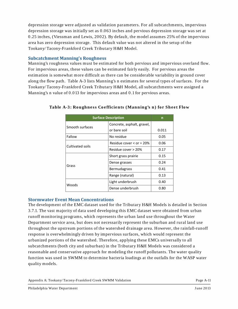
Subcatchment Manning's Roughness Manning’s roughness values must be estimated for both pervious and impervious overland flow. For impervious areas, these values can be estimated fairly easily. For pervious areas the estimation is somewhat more difficult as there can be considerable variability in ground cover along the flow path. Table A-3 lists Manning’s n estimates for several types of surfaces. For the Tookany/Tacony-Frankford Creek Tributary H&H Model, all subcatchments were assigned a Manning’s n value of 0.013 for impervious areas and 0.1 for pervious areas.
Table A-3: Roughness Coefficients (Manning’s n) for Sheet Flow
Source: US Department of Agriculture, June 1986
Stormwater Event Mean Concentrations The development of the EMC dataset used for the Tributary H&H Models is detailed in Section 3.7.1. The vast majority of data used developing this EMC dataset were obtained from urban runoff monitoring programs, which represents the urban land use throughout the Water Department service area, but does not necessarily represent the suburban and rural land use throughout the upstream portions of the watershed drainage area. However, the rainfall-runoff response is overwhelmingly driven by impervious surfaces, which would represent the urbanized portions of the watershed. Therefore, applying these EMCs universally to all subcatchments (both city and suburban) in the Tributary H&H Models was considered a reasonable and conservative approach for modeling the runoff pollutants. The water quality function was used in SWMM to determine bacteria loadings at the outfalls for the WASP water quality models.
Surface Description n
Smooth surfaces Concrete, asphalt, gravel, or bare soil 0.011
Fallow No residue 0.05
Cultivated soils Residue cover < or = 20% 0.06
Residue cover > 20% 0.17
Grass
Short grass prairie 0.15 Dense grasses 0.24 Bermudagrass 0.41 Range (natural) 0.13
Woods Light underbrush 0.40 Dense underbrush 0.80
Appendix A: Tookany/Tacony-Frankford Creek SWMM Validation Page A-12 Philadelphia Water Department June 2013
A.3.3 Model Input Precipitation Radar rainfall was obtained from Vieux & Associates, Inc. and processed to be used for the hydrologic validation period (years 2010 and 2012) and the water quality validation period (years 2003 and 2004). The radar grid was calibrated to the existing Water Department rain gage network, consisting of 24 gages within the City limits. Precipitation for each model subcatchment was calculated by area weighting 1 km2 radar grids intersecting the individual subcatchment boundaries. The radar rainfall data was necessary to provide coverage for sheds outside the coverage of the Water Department gage network. This improved the simulation of events with complex hydrographs and quick runoff responses. In a rainfall-runoff model, much of the uncertainty in the model results from the uncertainty inherent in the precipitation data. Therefore, using a detailed precipitation input that accounts for the temporal and spatial distribution in rainfall intensities and volumes, increases the accuracy and precision of the model results. Compared to using the Water Department rain gage network directly, radar rainfall has the potential to better represent the spatial distribution of rainfall between gages within the City, and for locations outside the rain gage network.
Evaporation Evaporation data was loaded into the model in the form of average monthly evaporation rates. Evaporation data usually can be obtained from the National Weather Service or from other pan measurements, however, long-term daily evaporation data was limited in the Philadelphia area. Neither the Philadelphia Airport nor the Wilmington Airport recorded evaporation data. One site located in New Castle County, Delaware recorded daily evaporation data from 1956 through 1994. Average daily evaporation (inches per day) from this site was used to estimate typical monthly evaporation rates, which were used by the model.
Baseflow Baseflow is required for each tributary in order to perform the in-stream hydrological validation of the watershed models. An estimate of baseflow was calculated using USGS gages 01467086 and 01467807. Baseflow is mostly comprised of groundwater discharge to the stream, while runoff is a result of overland discharge. Baseflow separation involved disaggregating monitored flow time series into wet and dry components based upon expected hydrological response times. In order to extract a baseflow from monitored streamflow data, the data set was first merged with rainfall data. All data during wet weather and 72 hours afterwards was removed to isolate dry weather flows. An average annual baseflow was estimated and used as a dry weather input to the model. The dry weather flow was weighted by contributing watershed area. Baseflow values were controlled within SWMM as multipliers on a constant dry weather inflow at the inflow nodes.
Boundary Condition Tide elevation data was needed where the Frankford Creek meets the Delaware River to provide an accurate head boundary. Since the Torresdale Avenue dam was the most downstream extent of the water quality modeling effort, the mean tide value from NOAA tide data was used as the ultimate boundary condition at the Delaware River. However, the model should be updated with
Appendix A: Tookany/Tacony-Frankford Creek SWMM Validation Page A-13 Philadelphia Water Department June 2013
a tidal time series if it is to be used to simulate the tidal portion of the Tookany/Tacony-Frankford Creek.
A.4 Validation
A.4.1 Validation Approach Validation of the Tributary H&H Model was performed using flow data collected at USGS monitoring locations along the Tookany/Tacony-Frankford Creek. Flow monitoring data was available for the 2010-2012 validation period. Initial estimates of selected variables were adjusted within a specified range until a satisfactory correlation between simulated and measured streamflow, over a range of events, was obtained. Stormwater runoff and the associated pollutant loadings from the watershed areas, including the stormwater contributions from separate sanitary sewered areas, were input to the Tributary H&H Model at nodes along the tributary networks. Flow from CSOs upstream of the USGS gaging stations is captured in the streamflow data, so was therefore a part of the validation dataset. However, flow from CSOs was considered fixed by the overflow validation process in the CSS Model, and therefore CSO shed parameters were not adjusted during validation of the Tributary H&H Model.
As discussed in Section A.3.2, runoff in SWMM is generated when the precipitation exceeds the demands of infiltration, evaporation, and storage. The rate of runoff is determined by the subcatchment area, width, slope, depth of the non-linear reservoir, and the roughness coefficient. Subcatchment area, slope, and total impervious area are quantifiable parameters and, therefore, were not adjusted during the validation process. Infiltration parameters, width, and percent routed were the primary parameters adjusted during validation. In addition, depression storage and overland roughness coefficients were adjusted during the validation process. Depression storage and overland roughness parameters were set independently for the pervious and impervious portions of the subcatchments.
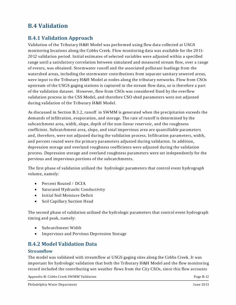
The first phase of validation utilized the hydrologic parameters that control event hydrograph volume, namely:
• Percent Routed / DCIA • Saturated Hydraulic Conductivity • Initial Soil Moisture Deficit • Soil Capillary Suction Head
The second phase of validation utilized the hydrologic parameters that control event hydrograph timing and peak, namely:
• Subcatchment Width • Impervious and Pervious Depression Storage
Appendix A: Tookany/Tacony-Frankford Creek SWMM Validation Page A-14 Philadelphia Water Department June 2013
A.4.2 Model Validation Data Streamflow The model was validated with streamflow at USGS gaging sites along the Tookany/Tacony-Frankford Creek. It was important for hydrologic validation that both the Tributary H&H Model and the flow monitoring record included the contributing wet weather flows from the City CSOs, since this flow accounts for a sizable portion of the streamflow in this urban stream. Instantaneous USGS flow monitoring data in 15 minute intervals was available over recent time periods for two gages along the Tookany/Tacony-Frankford Creek.
Presently there are two gages along the Tookany/Tacony-Frankford Creek, 01467086 and 01467087. Gage 01467086, located near the Adams Avenue bridge, is the more upstream gage and near where the stream passes through the City border. Gage 01467087 at the Castor Avenue bridge is the more downstream gage. The Castor Avenue gage is approximately 2.8 miles upstream of the mouth of the stream at the Delaware River and above the influence of tide. Current USGS gage data from 2010 through 2012 was used in favor of historical daily records for hydrologic validation. Current data better represents existing wet weather response of the watershed. The data is recorded in 15 minute increments, which provides a finer resolution for hydrographs.
USGS gage 01467086 has a well defined rating curve with wet weather flows up to 2000 cfs. Flows from this USGS gage were used to calibrate the model primarily outside the City. USGS gage 01467087 has a poorly defined rating curve. The peak field measured flow rate is about 2000 cfs. Field notes for this point report the reading as “poor”. The next highest recorded point is 158 cfs. Since the downstream gage 01467087 at Castor Avenue is the only active gage during the water quality validation period (2003-2004), and a water quality sampling station exists at the gage site, it was not excluded in the current year validation. The upper gage 01467086 was used to validate the modeled watershed areas outside the City, and the lower gage was used to validate the watershed areas below the upstream gage. Section 2.2.2 contains additional discussion of USGS gage station rating curve development and published flow data error ranges.
Event Definition Wet weather events were defined for each monitored dataset using the flow and precipitation monitoring records. A total of 146 events were defined for both gages within the hydrologic validation period of January 2010 through December 2012. The monitored and predicted hydrographs were split into discrete wet weather events over time, so comparisons could be made on an event by event basis. Events were defined not by continuous rainfall, but continuous wet weather response. Additionally, since snowmelt was not simulated, snowfall and all potential snow-melt events were removed from the validation data set.
During the validation process, each of these events was evaluated repeatedly to compare the observed and simulated event statistics for event volume and peak flow. The observed and simulated hydrographs were compared for their general response shape and timing. During the validation process, the model hydrologic parameters were adjusted to provide a better fit between the simulated and monitored flows. Care was taken to exclude the influence of events
Appendix A: Tookany/Tacony-Frankford Creek SWMM Validation Page A-15 Philadelphia Water Department June 2013
which had unusually large or small responses to the rainfall hyetograph so that the overall model validation would not be skewed by a select number of events. The ratio of monitored flow to precipitation volume over the contributing watershed area was also used as a reason to exclude events from the validation process. If there seemed to be a mismatch between rainfall and runoff response or hydrograph shape and timing, the event was deemed an outlier.
A.4.3 Validation Results Flow monitoring data from USGS stations 01467087 Frankford Creek at Castor Avenue and 01467086 Tacony Creek above Adams Avenue were used to perform the hydrologic validation of the Tookany/Tacony-Frankford Creek Tributary H&H Model. The upstream gage, 01467086 at Adams Avenue, is close to the City border and was used to validate the more upstream sheds that mostly lie outside the City and the Water Department service area. The downstream gage, 01467087 at Castor Avenue, was used to perform the hydrologic validation for the watershed area below the Adams Avenue gage. Flow data at this gage was used with caution since there is limited field measured flow data for large wet weather flows. USGS assigned a site rating condition of “poor” to this station. The rating curve includes more field measured flow rates of small and medium sized events and should provide a good representation of actual conditions in this range. Model flow time series were compared to observed flow for the events defined at both gages within the hydrologic validation period of January 2010 through December 2012.
Since the percent DCIA value was fixed as the total impervious area of the watershed subcatchments, it was not adjusted during validation. The model parameter adjusted to represent the effect of directly connected impervious areas was the “percent routed” parameter, since the pervious method of subcatchment routing was employed to represent the routing of runoff from impervious areas onto adjacent pervious areas. Through validation the percent routed parameter was determined to be 30% and was universally applied to all watershed subcatchments. This takes into account both the upstream and downstream gages.
A width of 10 times the square root of the shed area was assigned to the Tookany/Tacony-Frankford Creek watersheds. This value, which is larger than the initial area based estimates, was increased to reduce peak flows and to extend the simulated hydrograph.
The saturated hydraulic conductivity was adjusted to 0.30 in/hr for all sheds. This value was increased from the initial estimate based on the GIS soil information. The saturated hydraulic conductivity was first determined for the headwater sheds upstream of the Adams Avenue gage. Similar infiltration parameters were then applied to all sheds downstream of the gage and a reasonable fit was observed for the events at the Castor Avenue gage.
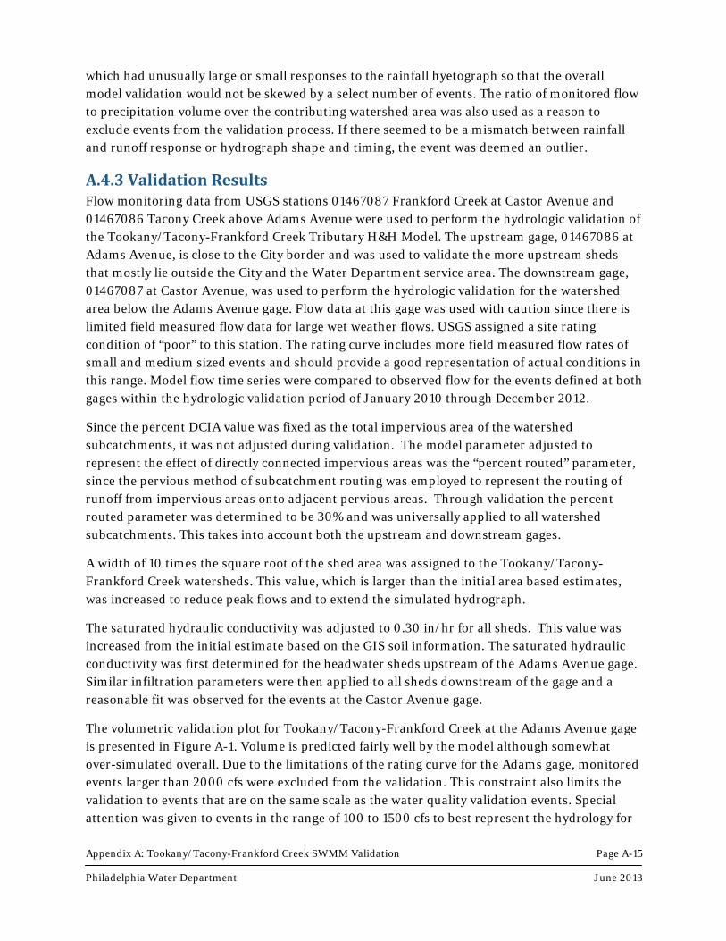
The volumetric validation plot for Tookany/Tacony-Frankford Creek at the Adams Avenue gage is presented in Figure A-1. Volume is predicted fairly well by the model although somewhat over-simulated overall. Due to the limitations of the rating curve for the Adams gage, monitored events larger than 2000 cfs were excluded from the validation. This constraint also limits the validation to events that are on the same scale as the water quality validation events. Special attention was given to events in the range of 100 to 1500 cfs to best represent the hydrology for
Appendix A: Tookany/Tacony-Frankford Creek SWMM Validation Page A-16 Philadelphia Water Department June 2013
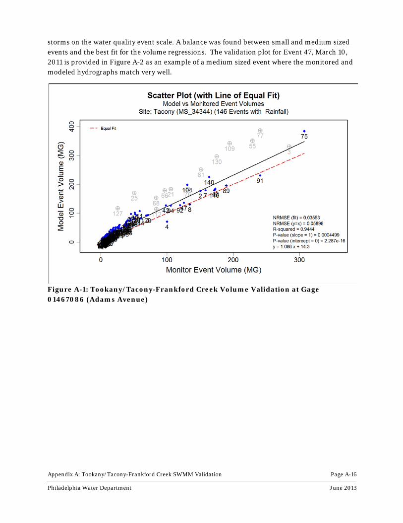
storms on the water quality event scale. A balance was found between small and medium sized events and the best fit for the volume regressions. The validation plot for Event 47, March 10, 2011 is provided in Figure A-2 as an example of a medium sized event where the monitored and modeled hydrographs match very well.
Figure A-1: Tookany/Tacony-Frankford Creek Volume Validation at Gage 01467086 (Adams Avenue)
Appendix A: Tookany/Tacony-Frankford Creek SWMM Validation Page A-17 Philadelphia Water Department June 2013
Figure A-2: Tookany/Tacony-Frankford Creek Example Validation Plot at Gage 01467086 (Adams Avenue)
Appendix A: Tookany/Tacony-Frankford Creek SWMM Validation Page A-18 Philadelphia Water Department June 2013
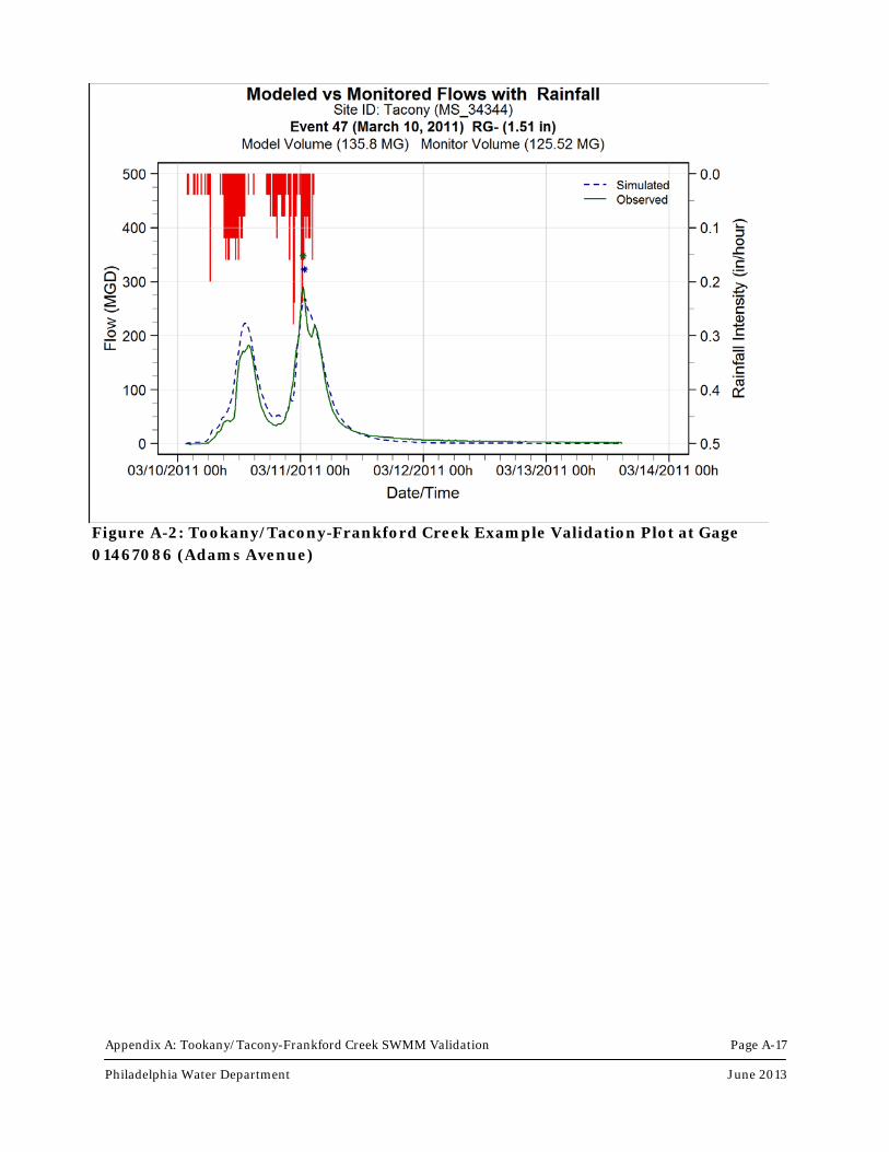
The volumetric validation plot for Tookany/Tacony-Frankford Creek at the Castor Avenue gage is presented in Figure A-3. Overall, the model does a good job of predicting volume. The regression is driven by one extreme event, however moderate and small-sized events seem to be simulated fairly well. These results suggest that the limitations of the rating curve for the Castor Avenue gage may not have a large impact on the overall validation for moderate and small events. The relatively good volume results at the Castor Avenue gage also suggest that the validation at the Adams Avenue gage was adequate. The validation plot for Event 140, October 28, 2012 is provided in Figure A-4 as an example of a medium to large-sized event where the monitored and modeled hydrographs match very well.
The validation results show that the model adequately represents the monitored data, and that overall it provides a good representation of the flows in Tookany/Tacony-Frankford Creek.
Figure A-3: Tookany/Tacony-Frankford Creek Volume Validation at Gage 01467087 (Castor Avenue)

Appendix A: Tookany/Tacony-Frankford Creek SWMM Validation Page A-19 Philadelphia Water Department June 2013
Figure A-4: Tookany/Tacony-Frankford Creek Example Validation Plot at Gage 01467087 (Castor Avenue)

Appendix A: Tookany/Tacony-Frankford Creek SWMM Validation Page A-20 Philadelphia Water Department June 2013
References US Environmental Protection Agency (US EPA), 2010. Storm Water Management Model (SWMM). <http://www.epa.gov/nrmrl/wswrd/wq/models/swmm/> (April 4, 2013).
Federal Emergency Management Agency, 2001. Flood Insurance Study: Montgomery County, Pennsylvania (All Jurisdictions).
Manning et al., 1987. Nationwide Evaluation of Combined Sewer Overflows and Urban Stormwater Discharges, Volume III: Characterization of Discharges, USEPA.
Philadelphia Water Department, 1997. CSO Documentation: Long Term Control Plan. <http://www.phillyriverinfo.org/CSOLTCPU/CSOLTCP/pdf/CSO%20LTCP.pdf> (May 9, 2013).
Philadelphia Water Department, 2005. Tookany/Tacony-Frankford Watershed Comprehensive Characterization Report. <http://www.phillywatersheds.org/doc/Tacony_Frankford_CCR.pdf> (May 9, 2013).
Philadelphia Water Department, 2008. Tookany/Tacony-Frankford Watershed Act 167 Stormwater Management Plan. <http://www.phillywatersheds.org/doc/TTF_Act167_Plan.pdf> (May 9, 2013).
Philadelphia Water Department, 2011. Green City Clean Waters. Philadelphia Water Department. <http://www.phillywatersheds.org/ltcpu/LTCPU_Complete.pdf> (May 9, 2013).
Stankowski, S.J, 1974. Magnitude and Frequency of Floods in New Jersey with Affects of Urbanization: NJDEP, Division of Water Resources, Special Report 38.
USDA, 1986. Urban Hydrology for Small Watersheds, TR-55.
Viessman, W. and Lewis, G.L, 2002. Introduction to Hydrology, 5th Edition. Prentice Hall.
Appendix B
Cobbs Creek SWMM Validation

Appendix B: Cobbs Creek SWMM Validation Page B-2 Philadelphia Water Department June 2013
B.1 Introduction This appendix describes the development and validation of the Cobbs Creek Tributary H&H Model used to provide the hydraulic and bacteria loadings to the United States Environmental Protection Agency (US EPA) Water Quality Analysis Simulation Program (WASP) model.
The US EPA Storm Water Management Model (SWMM) version 5 was used to develop the Combined Sewer System (CSS) Model and Watershed Model that together comprise the Tributary Hydraulic and Hydrologic (H&H) Model. SWMM5 hydrology, represented by subcatchments, simulated both the quantity and quality of runoff in a drainage basin and the routing of flows and contaminants to sewers or receiving waters. SWMM5 hydrology can accept precipitation (rainfall or snowfall) hyetographs and perform a step by step accounting of snowmelt, infiltration losses in pervious areas, surface detention, overland flow, and water quality constituents leading to the calculation of one or more hydrographs and/or pollutographs at a certain geographic point such as a sewer inlet. SWMM5 hydraulics, represented by nodes and links, simulates dynamic hydraulic flow routing and pollutant routing through open channel and closed conduit systems (US EPA, 2010).
The Cobbs Creek Tributary H&H Model was developed to simulate the stormwater runoff and water quality loading from combined sewer overflows (CSOs) and minor tributaries to the receiving waters. The model was developed primarily utilizing information obtained through previous modeling efforts and Geographic Information Systems (GIS) and was driven using continuous radar rainfall time series. Event mean concentrations (EMCs) were used to predict the stormwater quality components of the model. Flow validations were performed using monitoring records from United States Geological Survey (USGS) gaging stations. The model validation period of the Tributary H&H Model was dictated by available USGS stream flow and radar-rainfall data.
The following sections of this report further describe the models used in development and validation of the Cobbs Creek Tributary H&H Model.
B.2 Discussion of Legacy Models and Reports Several previously published models and reports were used to develop the Cobbs Creek Tributary H&H Model. This section discusses the role of legacy publications in model development.
B.2.1 Long Term Control Plan Update Combined Sewer System (CSS) Model The Southwest District combined sewer system of Philadelphia was originally modeled as part of the Long Term Control Plan (Philadelphia Water Department, 1997). Additional refinement of the CSS Model occurred as part of the Long Term Control Plan Update. CSS Model development and calibration methodology are discussed within Supplemental Documentation Volume 4 (Philadelphia Water Department, 2011).

Appendix B: Cobbs Creek SWMM Validation Page B-3 Philadelphia Water Department June 2013
The CSS Model domain included:
• The combined service area within the City borders, which drains to the Philadelphia Water Department (Water Department) Water Pollution Control Plants.
• The sanitary portion of the separate sewered area, within and outside the City, which drains to the Water Department Water Pollution Control Plants. A simplified version of the sanitary collection system is modeled inside the City, and indirectly modeled outside the City.
• The CSO and interceptor relief outfall pipes within the City, which discharge into the receiving waters.
B.2.2 HEC-2 Model An open channel HEC-2 model of Cobbs Creek was developed as part of a Federal Emergency Management Agency (FEMA) Flood Insurance Study (FIS). The Cobbs Creek HEC-2 Model was originally developed in 1974 (Federal Emergency Management Agency, 2001). Channel geometry data within the Cobbs Creek Watershed Model was supplemented with historic FEMA HEC-2 Model data.
B.2.3 Fluvial Geomorphology (FGM) Study Fluvial geomorphology data was collected as part of the Darby-Cobbs Creek Watershed Comprehensive Characterization Report (Philadelphia Water Department, 2004). Channel geometry and bed roughness data derived in the FGM study were used in development of the Cobbs Creek Watershed Model.
B.2.4 Act 167 Stormwater Management Plan A coupled CSS and Watershed Model of Cobbs Creek was developed as part of the Darby-Cobbs Creeks Act 167 Stormwater Management Plan (Philadelphia Water Department, 2008). The Southwest District CSS Model was integrated into a model of the Darby-Cobbs Creek watershed. Outfall pipes from the regulator structures in the CSS Model were connected to open channel nodes of the Watershed Model so wet weather overflows could be routed to the Cobbs Creek. The result was a model that included the collection system pipe network and all upstream inputs. The model developed for the Act 167 Plan served as the starting point for Tributary H&H Model development.
The Act 167 Model domain included:
• The combined service area within the City borders, which drains to the Water Department Water Pollution Control Plants.
• The sanitary portion of the separate sewered area, within and outside the City, which drains to the Water Department Water Pollution Control Plants. A simplified version of the sanitary collection system is modeled inside the City, and indirectly modeled outside the City.
• The combined sewer overflow and interceptor relief outfall pipes within the City, which discharge into receiving waters.
Appendix B: Cobbs Creek SWMM Validation Page B-4 Philadelphia Water Department June 2013
• Open channel representations of the receiving waters and major tributaries within the watershed.
• The stormwater and direct runoff areas within and outside of the City borders. Stormwater collection system conduits are not explicitly modeled.
B.3 Model Development The coupled CSS and Watershed Model of Cobbs Creek developed as part of the Cobbs Creek Act 167 Plan report served as the starting point for Tributary H&H Model development. The Act 167 Model was simplified by removing bridges, short culverts, and short cross sections. This simplification also improved model stability. The simplified model is referred to as the Tributary H&H Model and was validated against two USGS stream gages. This model provides the hydraulic and bacteria loadings to the WASP model.
The Cobbs Creek Tributary H&H Model includes the entire stream drainage area and extends beyond the Water Department service area and into Delaware and Montgomery Counties. The model representation of both the channel and the watershed areas beyond the Water Department service area was intended to capture the water quality effect of both East and West Indian Creeks. Figure 1-6 shows the model extents, subwatershed areas, and locations of Water Department and municipal collection system CSOs within the watershed area. In addition to the main channel of Cobbs Creek, the stream Naylor's Run was represented in the model to control and improve the timing and shape of the simulated hydrograph at the validation locations.
Within the City, both combined sewer and sanitary sewered areas are included in the Tributary H&H Model. Watershed areas outside the City and outside the CSS are also accounted for in the model. The non-combined sewer areas are mostly within the communities neighboring the City of Philadelphia to the north and west. These areas contribute runoff and associated pollutant loads to the receiving waters either through stormwater collection systems, direct runoff, or through minor tributary waterways.
B.3.1 Hydraulic Model Development SWMM5 uses a link-node description of sewer and open channel systems facilitating the physical prototype and the mathematical solution of the gradually-varied unsteady flow (St. Venant) equations which form the mathematical basis of the model. The links transmit the flow from node to node. Properties associated with the links include roughness, length, cross-sectional area, hydraulic radius, and surface width. The primary dependent variable for the links is discharge. Variables associated with nodes include volume, head, and surface area. The primary dependent variable for nodes is head, which is assumed to be changing in time, but constant throughout any one node.

Appendix B: Cobbs Creek SWMM Validation Page B-5 Philadelphia Water Department June 2013
Open Chanel Cross Sections The hydraulic network consisted of open channel representations of the Cobbs Creek and major tributaries within the watershed. It was developed from two separate data sets:
• Cross sectional data from HEC-2 models used in the Philadelphia County FIS
• Cross sectional data obtained through the FGM Study
The Water Department surveyed cross sections were used as the main channel for the Cobbs Creek Act 167 Model; the Act 167 Model was the starting point for development of the open channel portion of the Tributary H&H Model. At each of the surveyed locations, detailed profiles of the stream cross section were taken and two rebars were installed to mark each. The cross sections were extended out beyond the 100-year flood plain using GIS data. For cross sections that lie within the City of Philadelphia, a 1/3rd arc-second digital elevation model (DEM) was used. For cross sections that fell outside of the City boundaries, a 1 arc-second DEM was used. Cross sections were also drawn for the top decks of bridges and culverts to model flood conditions in the Act 167 Plan. However, these bridges and short culverts were removed to improve model stability in the Tributary H&H Model.
Cross sections from the HEC-2 Model of the Cobbs Creek used in the Philadelphia County FIS was used to supplement the Water Department survey. The HEC-2 Model was created to evaluate potential flooding in Cobbs Creek and included detailed cross sectional data of potential flow obstructions including dams and roadway/railway bridges. The cross sectional data was converted to City datum and formatted for use by SWMM5. Where the two data sets overlapped, cross sections were compared. The two models agreed fairly well so it was assumed HEC-2 cross sections, while less accurate, were a reasonable approximation. All Water Department surveyed cross sections along the main stem of the Cobbs Creek were sorted by river mile and connected.
The resultant tributary channel network consisted of over 100 channel cross sections representing more than 16 miles of stream. Since conduit length is the primary constraint when stabilizing a model, some conduits were replaced with lengthened equivalent conduits before being put into the model. However, this was done only when necessary. The Act 167 Model contains documentation of extended reaches. In the Cobbs Creek Tributary H&H Model, bridge crossings, most culverts, and short channels were consolidated and simplified to longer open channel conduits. The hydraulic configurations of the stream are based upon the best available information, but should not be considered a truly accurate depiction of actual stream conditions beyond the objectives of the water quality modeling tasks.
All elevations within the model are based on inverts calculated from the topographic contours and surveyed cross sections. Ground elevations are set as the maximum elevation found in the station elevation pairs defining any natural cross section. They are sufficiently high to prevent the hydraulic grade line within the channel from exceeding the user defined channel elevation.
The Water Department pebble counts along Cobbs Creek were used to estimate the value for Manning’s roughness within the channel. Channel roughness values for the Cobbs Creek were
Appendix B: Cobbs Creek SWMM Validation Page B-6 Philadelphia Water Department June 2013
assigned at all Water Department channel survey points. These roughness values are assumed to be representative until the next upstream survey point.
Floodplain roughness values for the transects were estimated from ortho-photography, field photographs at all Water Department survey points. These values are assumed to be representative until the next upstream survey point.
B.3.2 Hydrologic Model Development Subcatchment Delineation Subcatchment areas outside of the City were delineated by analyzing 1/3rd arc-second DEM to identify drainage divides. Further subdelineations at the subcatchment level were implied from topography, since limited to no collection system information was available. While, in general, subcatchment areas can be defined by surface topography, this is not always the case as subsurface drainage systems (sewers) can cross surface topographic divides. Subcatchment watersheds were delineated to selected points along the main channel at critical stream junctions or at pre-defined intervals. Since runoff from combined areas reaches the receiving water as a CSO input, sheds were defined for any watershed area not defined as a CSO subcatchment in the CSS Model. In this way runoff from areas defined as sanitary service areas, storm sheds, and non-contributing areas (to the collection system) was included in the Watershed Model. The defined sub-watersheds serve as the modeling unit in the Tributary H&H Model.
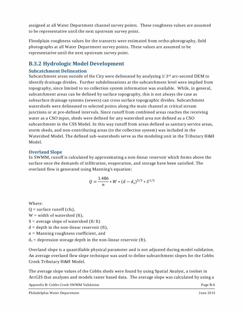
Overland Slope In SWMM, runoff is calculated by approximating a non-linear reservoir which forms above the surface once the demands of infiltration, evaporation, and storage have been satisfied. The overland flow is generated using Manning’s equation:
Where: Q = surface runoff (cfs), W = width of watershed (ft), S = average slope of watershed (ft/ft) d = depth in the non-linear reservoir (ft), n = Manning roughness coefficient, and
ds = depression storage depth in the non-linear reservoir (ft).
Overland slope is a quantifiable physical parameter and is not adjusted during model validation. An average overland flow slope technique was used to define subcatchment slopes for the Cobbs Creek Tributary H&H Model.
The average slope values of the Cobbs sheds were found by using Spatial Analyst, a toolset in ArcGIS that analyzes and models raster based data. The average slope was calculated by using a
Appendix B: Cobbs Creek SWMM Validation Page B-7 Philadelphia Water Department June 2013
1/3rd arc-second DEM that was bounded by a polygon feature class representation of the model subcatchments. Within Spatial Analyst, the "Slope" function calculates the maximum rate of change in value from that cell to its neighbors. For this analysis, the percent slope was calculated and redrawn as a new raster file. The "Zonal Statistics" function was then used to average the slope values within the shed boundaries.
Width The width parameter impacts the time of concentration and the hydrograph shape in the hydrologic portion of SWMM. Subcatchments are represented as rectangular areas defined by the subcatchment width parameter. By definition, the width of a watershed is equal to the area of the watershed divided by the length of the overland flow path. The width parameter is one of the main validation parameters used to adjust hydrograph shape, and to some degree hydrograph volume. Watersheds assigned a large width, and therefore a small overland flow length, will have a short time of concentration. Reducing width increases the flow length and will thus increase the time of concentration. Increasing the overland flow length also reduces the runoff volume as the flow is exposed to evaporation and infiltration over pervious areas for a longer period of time. Stormwater collection systems and minor undefined waterways are examples of how the overland flow length can be shortened, and the width increased. Overland flow length is a more intuitive parameter, and therefore is used as the basis for adjusting and discussing the SWMM width parameter. Since the width parameter is adjusted during validation, it is only necessary to obtain an approximate initial value.
The initial estimates for watershed width were obtained by calculating two times the square root of the watershed area. This approach provides a width based on an idealized square watershed along the middle of the watershed. Since actual watersheds are not rectangular with properties of symmetry and uniformity, it should be expected that these values will be widely adjusted during the validation process.
Gross Impervious Cover Gross percent impervious area was estimated from the 2006 National Land Cover Database impervious land coverage. An estimate of total impervious area for model subcatchments was based on clipping the impervious surface coverage with the Cobbs Creek subcatchment shed coverage and calculating the percent impervious cover for each subcatchment.
The estimate of percent impervious cover of total shed area was entered into the model as percent impervious for each subcatchment and was kept constant during the tributary validation process. Gross impervious area was not adjusted during the validation process. The influence of impervious cover on total shed stormwater runoff was controlled by the percent routed parameter, which was considered to be the impervious runoff validation parameter and simulated the effect of directly connected impervious area (DCIA).
Percent Impervious Cover Routed SWMM5 simulates surface runoff from drainage areas using three “planes” of overland flow. One plane represents all impervious surfaces directly connected to the hydraulic system and included initial abstraction or surface detention storage (puddles, cracks, etc. which do not
Appendix B: Cobbs Creek SWMM Validation Page B-8 Philadelphia Water Department June 2013
permit immediate runoff). A second plane represents all pervious areas and impervious areas not directly connected to the hydraulic system. The third plane is defined as the fraction of the directly connected area that provides no detention storage and thus produces runoff immediately. Furthermore, a portion of the pervious runoff can be routed to the impervious surface (i.e. Pervious Routing), or a portion of the impervious runoff can be routed to the pervious surface (i.e. Impervious Routing). The runoff from the drainage area is the sum of the flow from the three planes, after considering internal routing.
Impervious surfaces, by definition, do not have an infiltration component. However, impervious surfaces are not always connected to a collection or conveyance system, and may instead route to a pervious surface where the runoff generated has the opportunity to infiltrate. The fraction of the total area that is impervious and drains directly to the collection or conveyance system is defined as DCIA. In SWMM, the “% Impervious” hydrologic parameter represents the gross impervious area as a percentage of the total shed area. The PERVIOUS method of subcatchment routing is used to approximate hydrograph flow paths from the subcatchments. When the PERVIOUS method is used, a value for the percent of total runoff from the impervious area that is routed over the remaining pervious area of the shed is defined. The remaining impervious area not routed is termed the DCIA, which drains directly to the collection and conveyance system. The PERVIOUS routing method allows for complex hydrographs to be reproduced as DCIA is manifested as a near immediate system response to precipitation, while the pervious area runoff may have a slower response.
Soils The rate of infiltration is a function of soil properties in the drainage area, ground slopes, and ground cover. The Green-Ampt method of calculating infiltration was employed for the Cobbs Creek Tributary H&H Model. The Green-Ampt equation for infiltration has physically based parameters that can be estimated based on soil characteristics. The soil parameters used in this method are: average capillary suction, saturated hydraulic conductivity, and the initial moisture deficit. In SWMM, pervious area runoff is generated when rainfall volume and intensity exceed the soil infiltration capacity and evaporation demands. Infiltration is primarily controlled by setting the soil saturated hydraulic conductivity, which is that rate at which water will infiltrate the soil after the soil has reached a point of saturation. By lowering the saturated hydraulic conductivity, the pervious area begins to generate runoff. Once the saturated hydraulic conductivity threshold for pervious runoff is found, additional increment adjustments downward tend to produce very significant responses. Therefore, saturated hydraulic conductivity was a primary validation parameter.
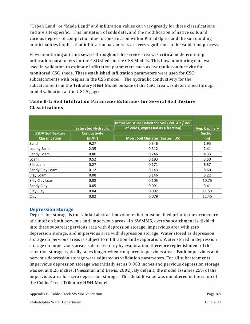
Soil information for the Cobbs watershed was obtained from the United States Department of Agriculture’s Natural Resources Conservation Service, which is responsible for collecting, storing, maintaining, and distributing soil survey information for lands in the United States. Infiltration parameters were assigned to each subcatchment based on soil texture classification. Table B-1 lists the parameter ranges for several different soil classifications. Soil classifications can vary widely within each subcatchment, and a weighted value was calculated for the three parameters. It should be noted that 80% of the Cobbs Creek watershed is classified as either
Appendix B: Cobbs Creek SWMM Validation Page B-9 Philadelphia Water Department June 2013
“Urban Land” or “Made Land” and infiltration values can vary greatly for these classifications and are site-specific. This limitation of soils data, and the modification of native soils and various degrees of compaction due to construction within Philadelphia and the surrounding municipalities implies that infiltration parameters are very significant in the validation process.
Flow monitoring at trunk sewers throughout the service area was critical in determining infiltration parameters for the CSO sheds in the CSS Models. This flow monitoring data was used in validation to estimate infiltration parameters such as hydraulic conductivity for monitored CSO sheds. These established infiltration parameters were used for CSO subcatchments with origins in the CSS model. The hydraulic conductivity for the subcatchments in the Tributary H&H Model outside of the CSO area was determined through model validation at the USGS gages.
Table B-1: Soil Infiltration Parameter Estimates for Several Soil Texture Classifications
USDA Soil Texture Classification
Saturated Hydraulic Conductivity
(in/hr)
Initial Moisture Deficit for Soil (Vol. Air / Vol. of Voids, expressed as a fraction) Avg. Capillary
Suction (in) Moist Soil Climates (Eastern US)
Sand 9.27 0.346 1.95 Loamy Sand 2.35 0.312 2.41 Sandy Loam 0.86 0.246 4.33 Loam 0.52 0.193 3.50 Silt Loam 0.27 0.171 6.57 Sandy Clay Loam 0.12 0.143 8.60 Clay Loam 0.08 0.146 8.22 Silty Clay Loam 0.08 0.105 10.75 Sandy Clay 0.05 0.091 9.41 Silty Clay 0.04 0.092 11.50 Clay 0.02 0.079 12.45 Depression Storage Depression storage is the rainfall abstraction volume that must be filled prior to the occurrence of runoff on both pervious and impervious areas. In SWMM5, every subcatchment is divided into three subareas: pervious area with depression storage, impervious area with zero depression storage, and impervious area with depression storage. Water stored as depression storage on pervious areas is subject to infiltration and evaporation. Water stored in depression storage on impervious areas is depleted only by evaporation, therefore replenishment of the retention storage typically takes longer when compared to pervious areas. Both impervious and pervious depression storage were adjusted as validation parameters. For all subcatchments, impervious depression storage was initially set as 0.063 inches and pervious depression storage was set at 0.25 inches, (Viessman and Lewis, 2002). By default, the model assumes 25% of the impervious area has zero depression storage. This default value was not altered in the setup of the Cobbs Creek Tributary H&H Model.
Appendix B: Cobbs Creek SWMM Validation Page B-10 Philadelphia Water Department June 2013
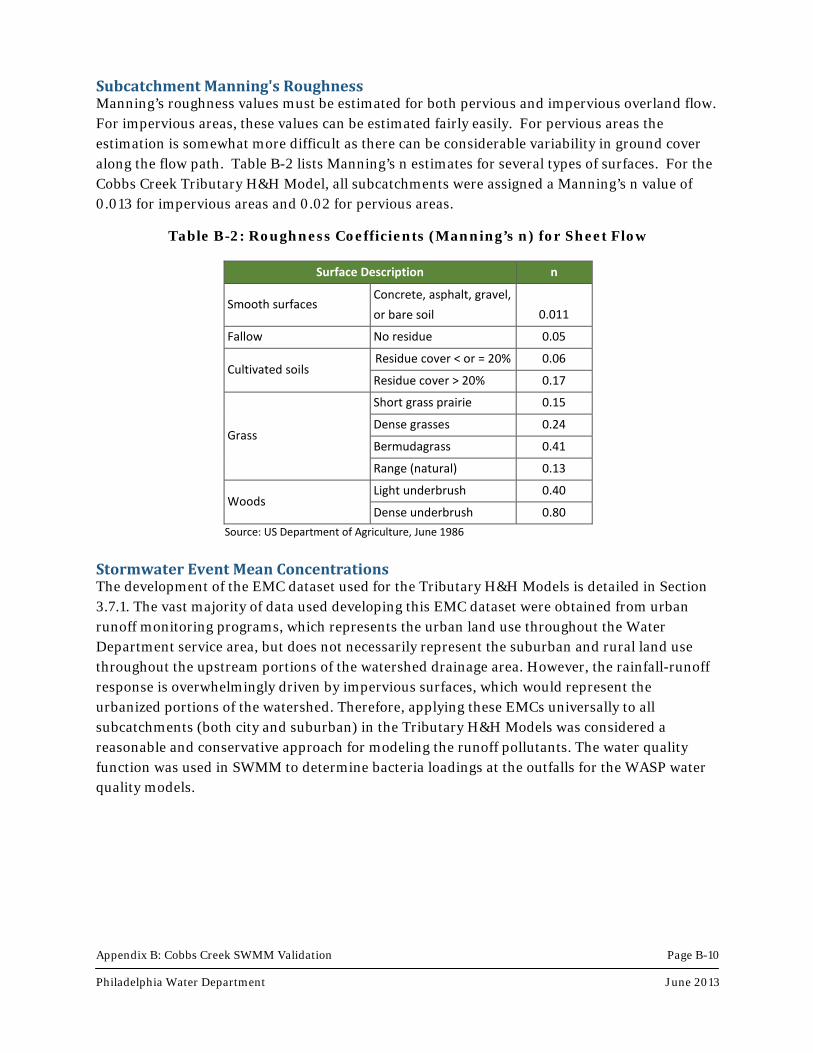
Subcatchment Manning's Roughness Manning’s roughness values must be estimated for both pervious and impervious overland flow. For impervious areas, these values can be estimated fairly easily. For pervious areas the estimation is somewhat more difficult as there can be considerable variability in ground cover along the flow path. Table B-2 lists Manning’s n estimates for several types of surfaces. For the Cobbs Creek Tributary H&H Model, all subcatchments were assigned a Manning’s n value of 0.013 for impervious areas and 0.02 for pervious areas.
Table B-2: Roughness Coefficients (Manning’s n) for Sheet Flow
Surface Description n
Smooth surfaces Concrete, asphalt, gravel, or bare soil 0.011
Fallow No residue 0.05
Cultivated soils Residue cover < or = 20% 0.06
Residue cover > 20% 0.17
Grass
Short grass prairie 0.15 Dense grasses 0.24 Bermudagrass 0.41 Range (natural) 0.13
Woods Light underbrush 0.40 Dense underbrush 0.80
Source: US Department of Agriculture, June 1986 Stormwater Event Mean Concentrations The development of the EMC dataset used for the Tributary H&H Models is detailed in Section 3.7.1. The vast majority of data used developing this EMC dataset were obtained from urban runoff monitoring programs, which represents the urban land use throughout the Water Department service area, but does not necessarily represent the suburban and rural land use throughout the upstream portions of the watershed drainage area. However, the rainfall-runoff response is overwhelmingly driven by impervious surfaces, which would represent the urbanized portions of the watershed. Therefore, applying these EMCs universally to all subcatchments (both city and suburban) in the Tributary H&H Models was considered a reasonable and conservative approach for modeling the runoff pollutants. The water quality function was used in SWMM to determine bacteria loadings at the outfalls for the WASP water quality models.
Appendix B: Cobbs Creek SWMM Validation Page B-11 Philadelphia Water Department June 2013
B.3.3 Model Input Precipitation Radar rainfall was obtained from Vieux & Associates, Inc. and processed to be used for the hydrologic validation period (years 2011 and 2012) and the water quality validation period (year 2003). The radar grid was calibrated to the existing Water Department rain gage network, consisting of 24 gages within the city limits. Precipitation for each model subcatchment was calculated by area weighting 1 km2 radar grids intersecting the individual subcatchment boundaries. The radar-rainfall data was necessary to provide coverage for sheds outside the coverage of the Water Department gage network. This improved the simulation of events with complex hydrographs and quick runoff responses. In a rainfall-runoff model, much of the uncertainty in the model results from the uncertainty inherent in the precipitation data. Therefore, using a detailed precipitation input that accounts for the temporal and spatial distribution in rainfall intensities and volumes, increases the accuracy and precision of the model results. Compared to using the Water Department rain gage network directly, radar rainfall has the potential to better represent the spatial distribution of rainfall between gages within the City, and for locations outside the rain gage network.
At the time of writing this report, the above mentioned radar rainfall data was not readily available for the year 2000 bacteria validation event for Cobbs Creek. For this event, instead of using radar rainfall to drive the model, the Water Department rain gage network was used directly.
Evaporation Evaporation data was loaded into the model in the form of average monthly evaporation rates. Evaporation data usually can be obtained from the National Weather Service or from other pan measurements, however, long-term daily evaporation data was limited in the Philadelphia area. Neither the Philadelphia Airport nor the Wilmington Airport recorded evaporation data. One site located in New Castle County, Delaware recorded daily evaporation data from 1956 through 1994. Average daily evaporation (inches per day) from this site was used to estimate typical monthly evaporation rates, which were used by the model.
Baseflow Baseflow is required for each tributary in order to perform the in-stream hydrological validation of the watershed models. An estimate of baseflow was calculated using USGS gage 01475548. Baseflow is mostly comprised of groundwater discharge to the stream, while runoff is a result of overland discharge. Baseflow separation involved disaggregating monitored flow time series into wet and dry components based upon expected hydrological response times. In order to extract a baseflow from monitored streamflow data, the data set was first merged with rainfall data. All data during wet weather and 72 hours afterwards was removed to isolate dry weather flows. An average annual baseflow was estimated and used as a dry weather input to the model. The dry weather flow was weighted by contributing watershed area. Baseflow values were controlled within SWMM5 as multipliers on a constant dry weather inflow at the inflow nodes.
Appendix B: Cobbs Creek SWMM Validation Page B-12 Philadelphia Water Department June 2013
B.4 Validation
B.4.1 Validation Approach Validation of the Tributary H&H Model was performed using flow data collected at USGS monitoring locations along the Cobbs Creek. Flow monitoring data was available for the 2011-2012 validation period. Initial estimates of selected variables were adjusted within a specified range until a satisfactory correlation between simulated and measured stream flow, over a range of events, was obtained. Stormwater runoff and the associated pollutant loadings from the watershed areas, including the stormwater contributions from separate sanitary sewered areas, were input to the Tributary H&H Model at nodes along the tributary networks. Flow from CSOs upstream of the USGS gaging stations is captured in the stream flow data, so is therefore a part of the validation dataset. However, flow from CSOs was considered fixed by the overflow validation process in the CSS Model, and therefore CSO shed parameters were not adjusted during validation of the Tributary H&H Model.
As discussed in Section B.3.2, runoff in SWMM is generated when the precipitation exceeds the demands of infiltration, evaporation, and storage. The rate of runoff is determined by the subcatchment area, width, slope, depth of the non-linear reservoir, and the roughness coefficient. Subcatchment area, slope, and total impervious area are quantifiable parameters and, therefore, were not adjusted during the validation process. Infiltration parameters, width, and percent routed were the primary parameters adjusted during validation. In addition, depression storage and overland roughness coefficients were adjusted during the validation process. Depression storage and overland roughness parameters were set independently for the pervious and impervious portions of the subcatchments.
The first phase of validation utilized the hydrologic parameters that control event hydrograph volume, namely:
• Percent Routed / DCIA • Saturated Hydraulic Conductivity • Initial Soil Moisture Deficit • Soil Capillary Suction Head
The second phase of validation utilized the hydrologic parameters that control event hydrograph timing and peak, namely:
• Subcatchment Width • Impervious and Pervious Depression Storage
B.4.2 Model Validation Data Streamflow The model was validated with streamflow at USGS gaging sites along the Cobbs Creek. It was important for hydrologic validation that both the Tributary H&H Model and the flow monitoring record included the contributing wet weather flows from the City CSOs, since this flow accounts

Appendix B: Cobbs Creek SWMM Validation Page B-13 Philadelphia Water Department June 2013
for a sizable portion of the stream flow in this urban stream. Instantaneous USGS flow monitoring data in 15 minute intervals was available over recent time periods for two gages along the Cobbs Creek.
Presently there are two gages along the Cobbs Creek, 01475530 and 01475548. Gage 01475530, located at the Route 1 bridge, is the more upstream gage and near where the stream passes through the City border. Gage 01475548 at the Mt. Moriah Cemetery is the more downstream gage. The Mt. Moriah gage is approximately two-thirds the river mile distance downstream of the Route. 1 gage to the mouth of the Cobbs Creek Watershed (confluence with Darby Creek) and above the influence of tide. Current USGS gage data from 2011 through 2012 was used in favor of historical daily records for hydrologic validation. Current data better represents existing wet weather response of the watershed. The data is recorded in 15 minute increments, which provides a finer resolution for hydrographs. Flows from the Route 1 gage were used to calibrate the model primarily outside the City, while the lower gage at Mt. Moriah was used to validate the watershed areas below the upstream gage. Section 2.2.2 contains additional discussion of USGS gage station rating curve development and published flow data error ranges.
Event Definition Wet weather events were defined for each monitored dataset using the flow and precipitation monitoring records. A total of 110 wet-weather events at USGS Gage 01475530 (Rt. 1), and 109 wet weather events at USGS Gage 01475548 (Mt. Moriah) were defined within the hydrologic validation period of January 2011 through December 2012. The monitored and predicted hydrographs were split into discrete wet weather events over time, so comparisons could be made on an event by event basis. Events were defined not by continuous rainfall, but continuous wet weather response. Additionally, since snowmelt was not simulated, snowfall and all potential snowmelt events were removed from the validation data set. This determination was based on precipitation and temperature data obtained from the Philadelphia International Airport.
The defined events were mostly similar in duration, except for small differences in event timing, and other differences due to the spatial distribution of rainfall. There was a higher percentage of pervious cover contributing to the upper gage at Route 1, so the events responded slower, with more prolonged wet weather tails. Consequently, a few of the events at Route 1 were merged, based on timing and extended wet weather tails, as compared to the Mt. Moriah events.
During the validation process, each of these events was evaluated repeatedly to compare the observed and simulated event statistics for event volume and peak flow. The observed and simulated hydrographs were compared for their general response shape and timing. During the validation process, the model hydrologic parameters were adjusted to provide a better fit between the simulated and monitored flows. Care was taken not to include the influence of events which had unusually large or small responses to the rainfall hyetograph so that the overall model validation would not be skewed by a select number of events. The ratio of monitored flow to precipitation volume over the contributing watershed area was also used as a reason to exclude events from the validation process. If there seemed to be a mismatch between rainfall and runoff response or hydrograph shape and timing, the event was deemed an outlier.
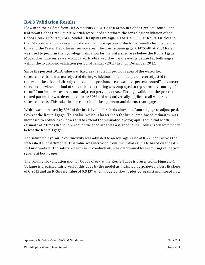
Appendix B: Cobbs Creek SWMM Validation Page B-14 Philadelphia Water Department June 2013
B.4.3 Validation Results Flow monitoring data from USGS stations USGS Gage 01475530 Cobbs Creek at Route 1 and 01475548 Cobbs Creek at Mt. Moriah were used to perform the hydrologic validation of the Cobbs Creek Tributary H&H Model. The upstream gage, Gage 01475530 at Route 1 is close to the City border and was used to validate the more upstream sheds that mostly lie outside the City and the Water Department service area. The downstream gage, 01475548 at Mt. Moriah was used to perform the hydrologic validation for the watershed area below the Route 1 gage. Model flow time series were compared to observed flow for the events defined at both gages within the hydrologic validation period of January 2011 through December 2012.
Since the percent DCIA value was fixed as the total impervious area of the watershed subcatchments, it was not adjusted during validation. The model parameter adjusted to represent the effect of directly connected impervious areas was the “percent routed” parameter, since the pervious method of subcatchment routing was employed to represent the routing of runoff from impervious areas onto adjacent pervious areas. Through validation the percent routed parameter was determined to be 30% and was universally applied to all watershed subcatchments. This takes into account both the upstream and downstream gages.
Width was increased by 50% of the initial value for sheds above the Route 1 gage to adjust peak flows at the Route 1 gage. This value, which is larger than the initial area-based estimates, was increased to reduce peak flows and to extend the simulated hydrograph. The initial width estimate of 2 times the square root of the shed area was assigned to the Cobbs Creek watersheds below the Route 1 gage.
The saturated hydraulic conductivity was adjusted to an average value of 0.22 in/hr across the watershed subcatchments. This value was increased from the initial estimate based on the GIS soil information. The saturated hydraulic conductivity was determined by examining validation results at both gages.
The volumetric validation plot for Cobbs Creek at the Route 1 gage is presented in Figure B-1. Volume is predicted fairly well at this gage by the model as indicated by achieved a best fit slope of 0.9515 and an R-Square value of 0.9137 when modeled flow is plotted against monitored flow.
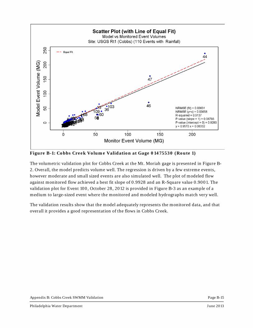
Appendix B: Cobbs Creek SWMM Validation Page B-15 Philadelphia Water Department June 2013
Figure B-1: Cobbs Creek Volume Validation at Gage 01475530 (Route 1)
The volumetric validation plot for Cobbs Creek at the Mt. Moriah gage is presented in Figure B-2. Overall, the model predicts volume well. The regression is driven by a few extreme events, however moderate and small sized events are also simulated well. The plot of modeled flow against monitored flow achieved a best fit slope of 0.9928 and an R-Square value 0.9001. The validation plot for Event 100, October 28, 2012 is provided in Figure B-3 as an example of a medium to large-sized event where the monitored and modeled hydrographs match very well.
The validation results show that the model adequately represents the monitored data, and that overall it provides a good representation of the flows in Cobbs Creek.
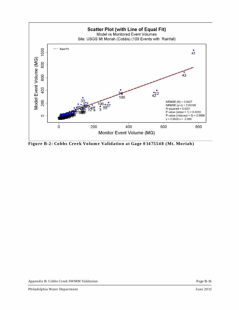
Appendix B: Cobbs Creek SWMM Validation Page B-16 Philadelphia Water Department June 2013
Figure B-2: Cobbs Creek Volume Validation at Gage 01475548 (Mt. Moriah)
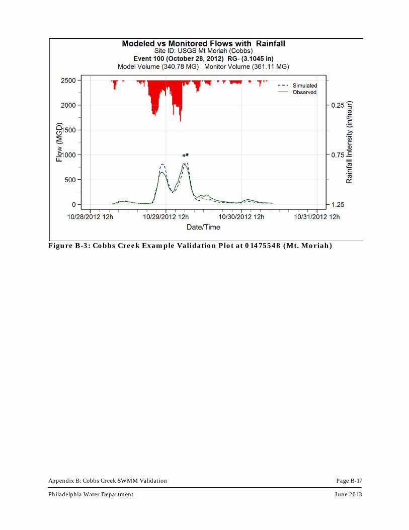
Appendix B: Cobbs Creek SWMM Validation Page B-17 Philadelphia Water Department June 2013
Figure B-3: Cobbs Creek Example Validation Plot at 01475548 (Mt. Moriah)

Appendix B: Cobbs Creek SWMM Validation Page B-18 Philadelphia Water Department June 2013
References
US Environmental Protection Agency (US EPA), 2010. Storm Water Management Model (SWMM). <http://www.epa.gov/nrmrl/wswrd/wq/models/swmm/> (April 4, 2013).
Federal Emergency Management Agency, 2001. Flood Insurance Study: Montgomery County, Pennsylvania (All Jurisdictions).
Philadelphia Water Department, 1997. CSO Documentation: Long Term Control Plan. <http://www.phillyriverinfo.org/CSOLTCPU/CSOLTCP/pdf/CSO%20LTCP.pdf> (May 9, 2013).
Philadelphia Water Department. 2004. Darby-Cobbs Watershed Comprehensive Characterization Report. <http://www.phillywatersheds.org/doc/DarbyCobbs_CCR.pdf> (May 9, 2013).
Philadelphia Water Department, 2008. Darby-Cobbs Creeks Watershed Act 167 Stormwater Management Plan. <http://www.phillywatersheds.org/doc/Darby_Cobbs_167.pdf> (May 9, 2013).
Philadelphia Water Department, 2011. Green City Clean Waters. Philadelphia Water Department. <http://www.phillywatersheds.org/ltcpu/LTCPU_Complete.pdf> (May 9, 2013).
USDA, 1986. Urban Hydrology for Small Watersheds, TR-55.
Viessman, W. and Lewis, G.L, 2002. Introduction to Hydrology, 5th Edition. Prentice Hall.
Appendix C
Tookany/Tacony-Frankford Creek
Bacteria Model Validation Simulations

Appendix C: Tacony Creek Bacteria Model Validation Simulations:
This report compares observed bacteria data and WASP predicted outputs for the following eight storms: May 06, 2003, May 07, 2003, May 16, 2003, July10, 2003, Sept 23, 2003, Oct 14, 2003, July 07, 2004, and Aug 30, 2004.
iii
Table of Contents 1. General Information ................................................................................................................................. 1
1.1. Segmentation Map .......................................................................................................................... 2 2. SWMM Model Validations ....................................................................................................................... 3
2.1. Modeled vs. Monitored Flows with Rainfall .................................................................................. 3 2.2. Validation Scatter Plots................................................................................................................... 7
3. E. coli ........................................................................................................................................................ 10 3.1. E. coli Time Series ........................................................................................................................ 10
3.1.1. May 06, 2003 Storm - TF280 ........................................................................................... 10 3.1.2. May 06, 2003 Storm - TF680 ........................................................................................... 11 3.1.3. May 06, 2003 Storm - TF975 ........................................................................................... 11 3.1.4. May 07, 2003 Storm - TF280 ........................................................................................... 12 3.1.5. May 07, 2003 Storm - TF680 ........................................................................................... 12 3.1.6. May 07, 2003 Storm - TF975 ........................................................................................... 13 3.1.7. May 16, 2003 Storm - TF280 ........................................................................................... 13 3.1.8. May 16, 2003 Storm - TF680 ........................................................................................... 14 3.1.9. May 16, 2003 Storm - TF975 ........................................................................................... 14 3.1.10. July 10, 2003 Storm - TF280 .......................................................................................... 15 3.1.11. July 10, 2003 Storm - TF680 .......................................................................................... 15 3.1.12. July 10, 2003 Storm - TF975 .......................................................................................... 16 3.1.13. Sept 23, 2003 Storm - TF280 ......................................................................................... 16 3.1.14. Sept 23, 2003 Storm - TF680 ......................................................................................... 17 3.1.15. Sept 23, 2003 Storm - TF975 ......................................................................................... 17 3.1.16. Oct 14, 2003 Storm - TF280........................................................................................... 18 3.1.17. Oct 14, 2003 Storm - TF680........................................................................................... 18 3.1.18. Oct 14, 2003 Storm - TF975........................................................................................... 19 3.1.19. July 07, 2004 Storm - TF280 .......................................................................................... 19 3.1.20. July 07, 2004 Storm - TF680 .......................................................................................... 20 3.1.21. July 07, 2004 Storm - TF975 .......................................................................................... 20 3.1.22. Aug 30, 2004 Storm - TF280 ......................................................................................... 21 3.1.23. Aug 30, 2004 Storm - TF680 ......................................................................................... 21 3.1.24. Aug 30, 2004 Storm - TF975 ......................................................................................... 22
3.2. E. coli and Flow Out Time Series ................................................................................................. 22 3.2.1. May 06, 2003 Storm - TF280 ........................................................................................... 22 3.2.2. May 06, 2003 Storm - TF680 ........................................................................................... 23 3.2.3. May 06, 2003 Storm - TF975 ........................................................................................... 23 3.2.4. May 07, 2003 Storm - TF280 ........................................................................................... 24 3.2.5. May 07, 2003 Storm - TF680 ........................................................................................... 24 3.2.6. May 07, 2003 Storm - TF975 ........................................................................................... 25 3.2.7. May 16, 2003 Storm - TF280 ........................................................................................... 25 3.2.8. May 16, 2003 Storm - TF680 ........................................................................................... 26 3.2.9. May 16, 2003 Storm - TF975 ........................................................................................... 26 3.2.10. July 10, 2003 Storm - TF280 .......................................................................................... 27 3.2.11. July 10, 2003 Storm - TF680 .......................................................................................... 27
iv
3.2.12. July 10, 2003 Storm - TF975 .......................................................................................... 28 3.2.13. Sept 23, 2003 Storm - TF280 ......................................................................................... 28 3.2.14. Sept 23, 2003 Storm - TF680 ......................................................................................... 29 3.2.15. Sept 23, 2003 Storm - TF975 ......................................................................................... 29 3.2.16. Oct 14, 2003 Storm - TF280........................................................................................... 30 3.2.17. Oct 14, 2003 Storm - TF680........................................................................................... 30 3.2.18. Oct 14, 2003 Storm - TF975........................................................................................... 31 3.2.19. July 07, 2004 Storm - TF280 .......................................................................................... 31 3.2.20. July 07, 2004 Storm - TF680 .......................................................................................... 32 3.2.21. July 07, 2004 Storm - TF975 .......................................................................................... 32 3.2.22. Aug 30, 2004 Storm - TF280 ......................................................................................... 33 3.2.23. Aug 30, 2004 Storm - TF680 ......................................................................................... 33 3.2.24. Aug 30, 2004 Storm - TF975 ......................................................................................... 34
3.3. Predicted and Observed E. coli Concentration Box Plots ............................................................. 35 3.3.1. E. coli Concentration for 2003-2004 Storms - TF280 ...................................................... 35 3.3.2. E. coli Concentration for 2003-2004 Storms - TF680 ...................................................... 35 3.3.3. E. coli Concentration for 2003-2004 Storms - TF975 ...................................................... 36 3.3.4. E. coli Concentration for 2003-2004 Storms - All Sites ................................................... 36
3.4. Predicted vs. Observed E. coli Load Scatter Plots ........................................................................ 37 3.4.1. E. coli Load for 2003-2004 Storms - TF280 .................................................................... 37 3.4.2. E. coli Load for 2003-2004 Storms - TF680 .................................................................... 38 3.4.3. E. coli Load for 2003-2004 Storms - TF975 .................................................................... 38 3.4.4. E. coli Load for 2003-2004 Storms - All Sites ................................................................. 39
3.5. Statistical Analysis - Observed Data ............................................................................................. 40 3.6. Statistical Analysis - Simulated Data ............................................................................................ 41
4. Fecal Coliform ......................................................................................................................................... 42 4.1. Fecal Coliform Time Series .......................................................................................................... 42
4.1.1. May 06, 2003 Storm - TF280 ........................................................................................... 42 4.1.2. May 06, 2003 Storm - TF680 ........................................................................................... 43 4.1.3. May 06, 2003 Storm - TF975 ........................................................................................... 43 4.1.4. May 07, 2003 Storm - TF280 ........................................................................................... 44 4.1.5. May 07, 2003 Storm - TF680 ........................................................................................... 44 4.1.6. May 07, 2003 Storm - TF975 ........................................................................................... 45 4.1.7. May 16, 2003 Storm - TF280 ........................................................................................... 45 4.1.8. May 16, 2003 Storm - TF680 ........................................................................................... 46 4.1.9. May 16, 2003 Storm - TF975 ........................................................................................... 46 4.1.10. July 10, 2003 Storm - TF280 .......................................................................................... 47 4.1.11. July 10, 2003 Storm - TF680 .......................................................................................... 47 4.1.12. July 10, 2003 Storm - TF975 .......................................................................................... 48 4.1.13. Sept 23, 2003 Storm - TF280 ......................................................................................... 48 4.1.14. Sept 23, 2003 Storm - TF680 ......................................................................................... 49 4.1.15. Sept 23, 2003 Storm - TF975 ......................................................................................... 49 4.1.16. Oct 14, 2003 Storm - TF280........................................................................................... 50 4.1.17. Oct 14, 2003 Storm - TF680........................................................................................... 50 4.1.18. Oct 14, 2003 Storm - TF975........................................................................................... 51 4.1.19. July 07, 2004 Storm - TF280 .......................................................................................... 51 4.1.20. July 07, 2004 Storm - TF680 .......................................................................................... 52
v
4.1.21. July 07, 2004 Storm - TF975 .......................................................................................... 52 4.1.22. Aug 30, 2004 Storm - TF280 ......................................................................................... 53 4.1.23. Aug 30, 2004 Storm - TF680 ......................................................................................... 53 4.1.24. Aug 30, 2004 Storm - TF975 ......................................................................................... 54
4.2. Fecal Coliform and Flow Out Time Series ................................................................................... 54 4.2.1. May 06, 2003 Storm - TF280 ........................................................................................... 54 4.2.2. May 06, 2003 Storm - TF680 ........................................................................................... 55 4.2.3. May 06, 2003 Storm - TF975 ........................................................................................... 55 4.2.4. May 07, 2003 Storm - TF280 ........................................................................................... 56 4.2.5. May 07, 2003 Storm - TF680 ........................................................................................... 56 4.2.6. May 07, 2003 Storm - TF975 ........................................................................................... 57 4.2.7. May 16, 2003 Storm - TF280 ........................................................................................... 57 4.2.8. May 16, 2003 Storm - TF680 ........................................................................................... 58 4.2.9. May 16, 2003 Storm - TF975 ........................................................................................... 58 4.2.10. July 10, 2003 Storm - TF280 .......................................................................................... 59 4.2.11. July 10, 2003 Storm - TF680 .......................................................................................... 59 4.2.12. July 10, 2003 Storm - TF975 .......................................................................................... 60 4.2.13. Sept 23, 2003 Storm - TF280 ......................................................................................... 60 4.2.14. Sept 23, 2003 Storm - TF680 ......................................................................................... 61 4.2.15. Sept 23, 2003 Storm - TF975 ......................................................................................... 61 4.2.16. Oct 14, 2003 Storm - TF280........................................................................................... 62 4.2.17. Oct 14, 2003 Storm - TF680........................................................................................... 62 4.2.18. Oct 14, 2003 Storm - TF975........................................................................................... 63 4.2.19. July 07, 2004 Storm - TF280 .......................................................................................... 63 4.2.20. July 07, 2004 Storm - TF680 .......................................................................................... 64 4.2.21. July 07, 2004 Storm - TF975 .......................................................................................... 64 4.2.22. Aug 30, 2004 Storm - TF280 ......................................................................................... 65 4.2.23. Aug 30, 2004 Storm - TF680 ......................................................................................... 65 4.2.24. Aug 30, 2004 Storm - TF975 ......................................................................................... 66
4.3. Predicted and Observed Fecal Coliform Concentration Box Plots ............................................... 67 4.3.1. Fecal Coliform Concentration for 2003-2004 Storms - TF280 ........................................ 67 4.3.2. Fecal Coliform Concentration for 2003-2004 Storms - TF680 ........................................ 68 4.3.3. Fecal Coliform Concentration for 2003-2004 Storms - TF975 ........................................ 69 4.3.4. Fecal Coliform Concentration for 2003-2004 Storms - All Sites ..................................... 70
4.4. Predicted vs. Observed Fecal Coliform Load Scatter Plots .......................................................... 70 4.4.1. Fecal Coliform Load for 2003-2004 Storms - TF280 ...................................................... 71 4.4.2. Fecal Coliform Load for 2003-2004 Storms - TF680 ...................................................... 71 4.4.3. Fecal Coliform Load for 2003-2004 Storms - TF975 ...................................................... 72 4.4.4. Fecal Coliform Load for 2003-2004 Storms - All Sites ................................................... 72
4.5. Statistical Analysis - Observed Data ............................................................................................. 73 4.6. Statistical Analysis - Simulated Data ............................................................................................ 74
vi
List of Tables 1-1. TTF Monitoring Locations ...................................................................................................................... 1 3-1. Total Rainfall and Peak Flow for Eight Storms .................................................................................... 37 3-2. E. coli - Observed Data Statistical Analysis .......................................................................................... 40 3-3. E. coli - Simulated Data Statistical Analysis ......................................................................................... 41 4-1. Total Rainfall and Peak Flow for Eight Storms .................................................................................... 70 4-2. Fecal Coliform - Observed Data Statistical Analysis ............................................................................ 73 4-3. Fecal Coliform - Simulated Data Statistical Analysis ........................................................................... 74
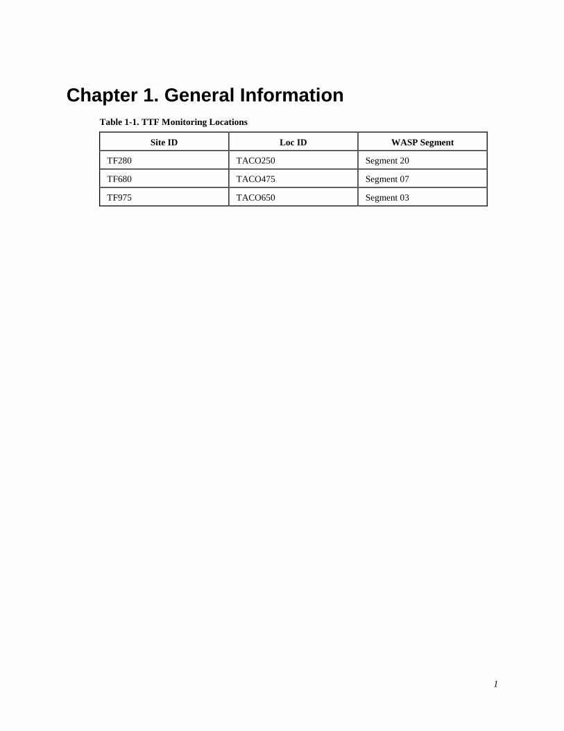
1
Chapter 1. General Information Table 1-1. TTF Monitoring Locations
Site ID Loc ID WASP Segment
TF280 TACO250 Segment 20
TF680 TACO475 Segment 07
TF975 TACO650 Segment 03
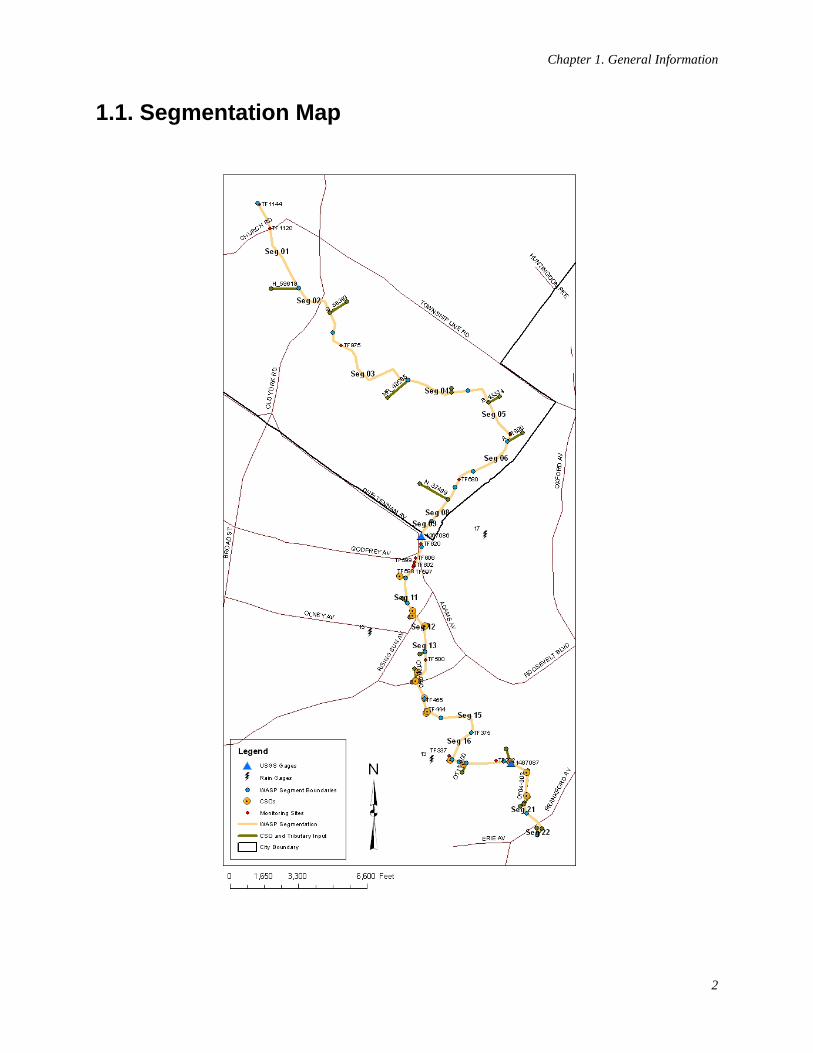
Chapter 1. General Information
2
1.1. Segmentation Map
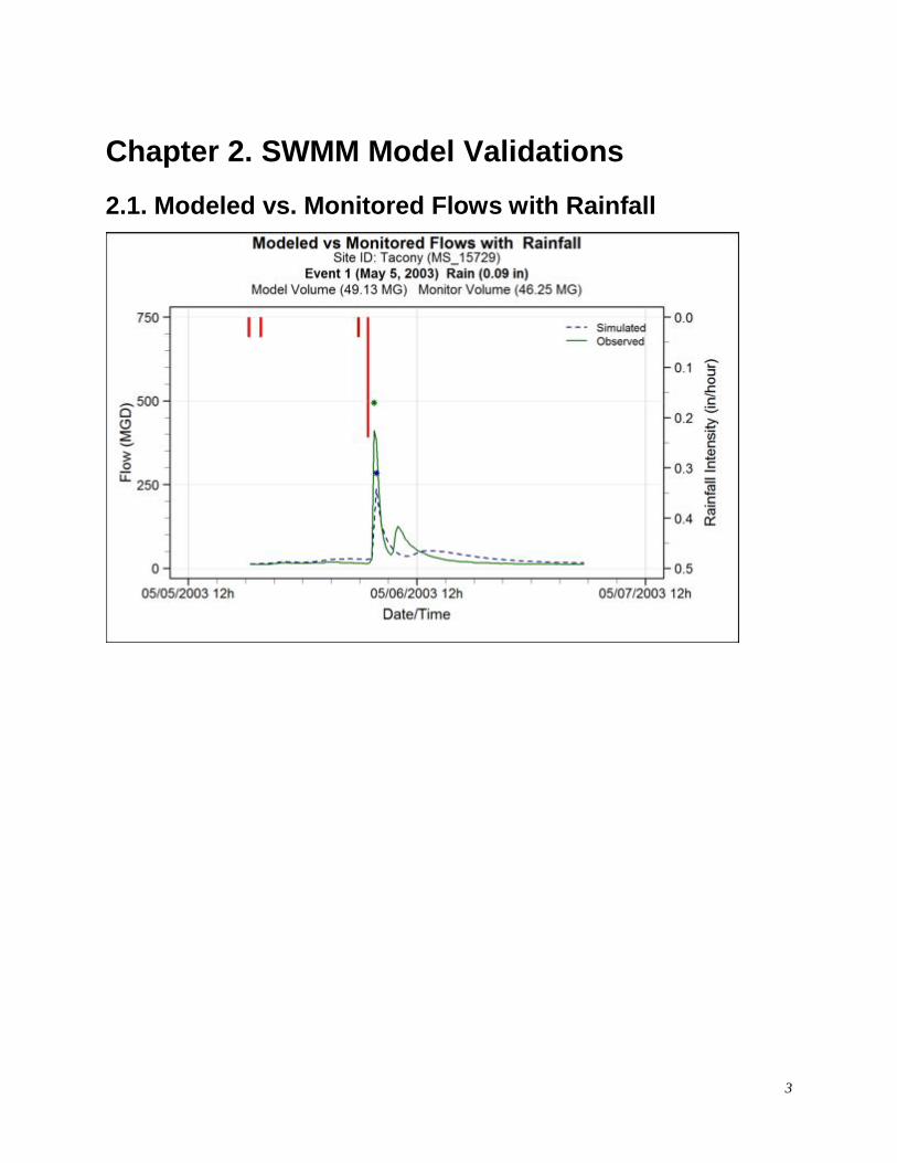
3
Chapter 2. SWMM Model Validations
2.1. Modeled vs. Monitored Flows with Rainfall
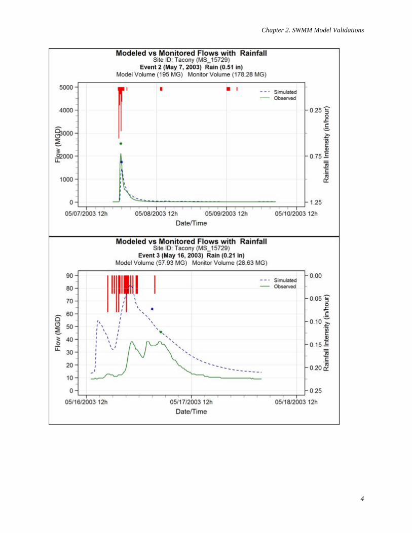
Chapter 2. SWMM Model Validations
4

Chapter 2. SWMM Model Validations
5
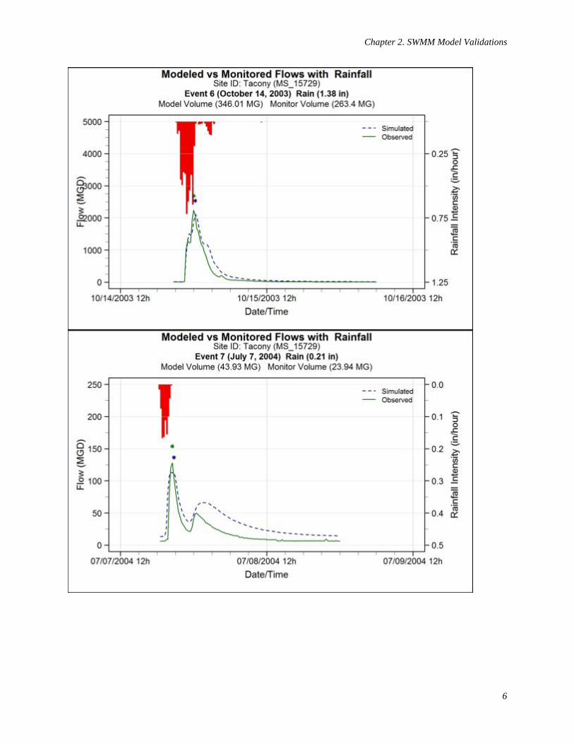
Chapter 2. SWMM Model Validations
6
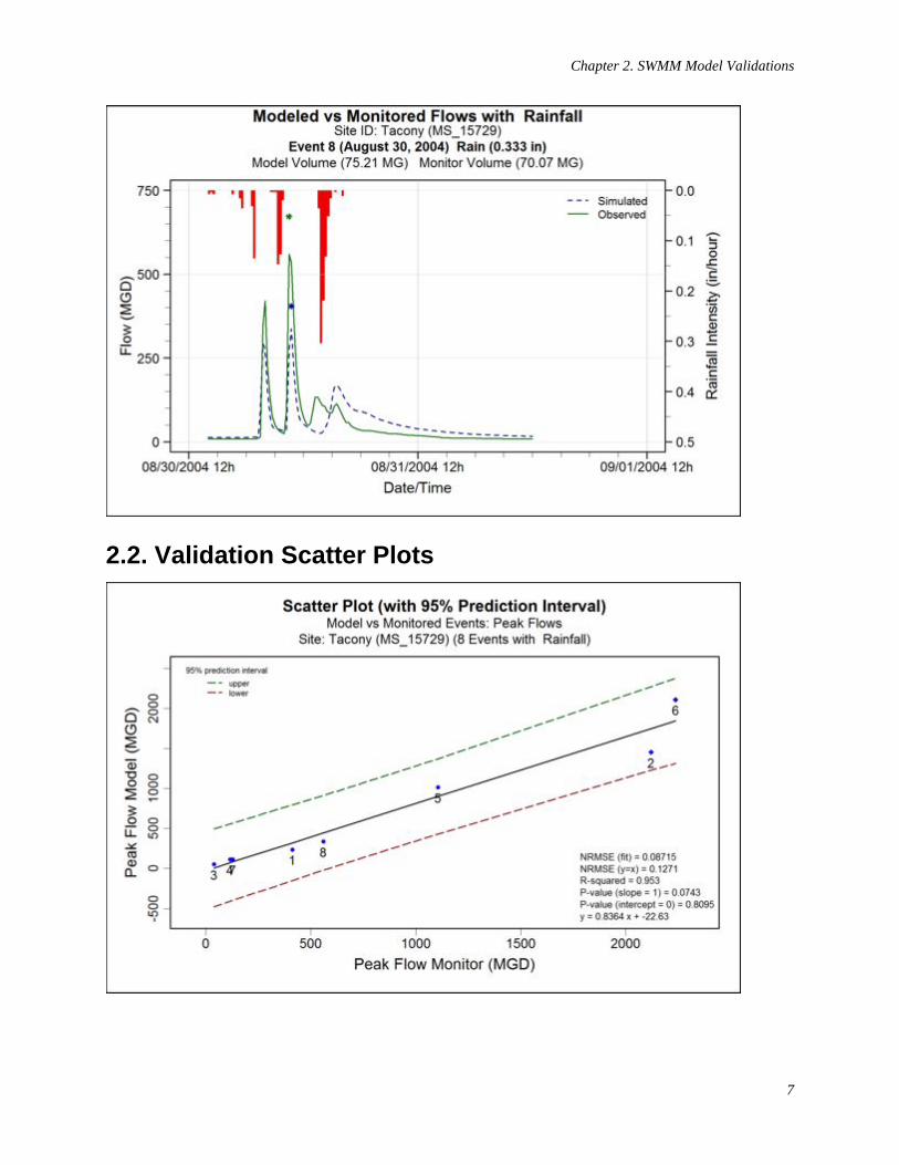
Chapter 2. SWMM Model Validations
7
2.2. Validation Scatter Plots
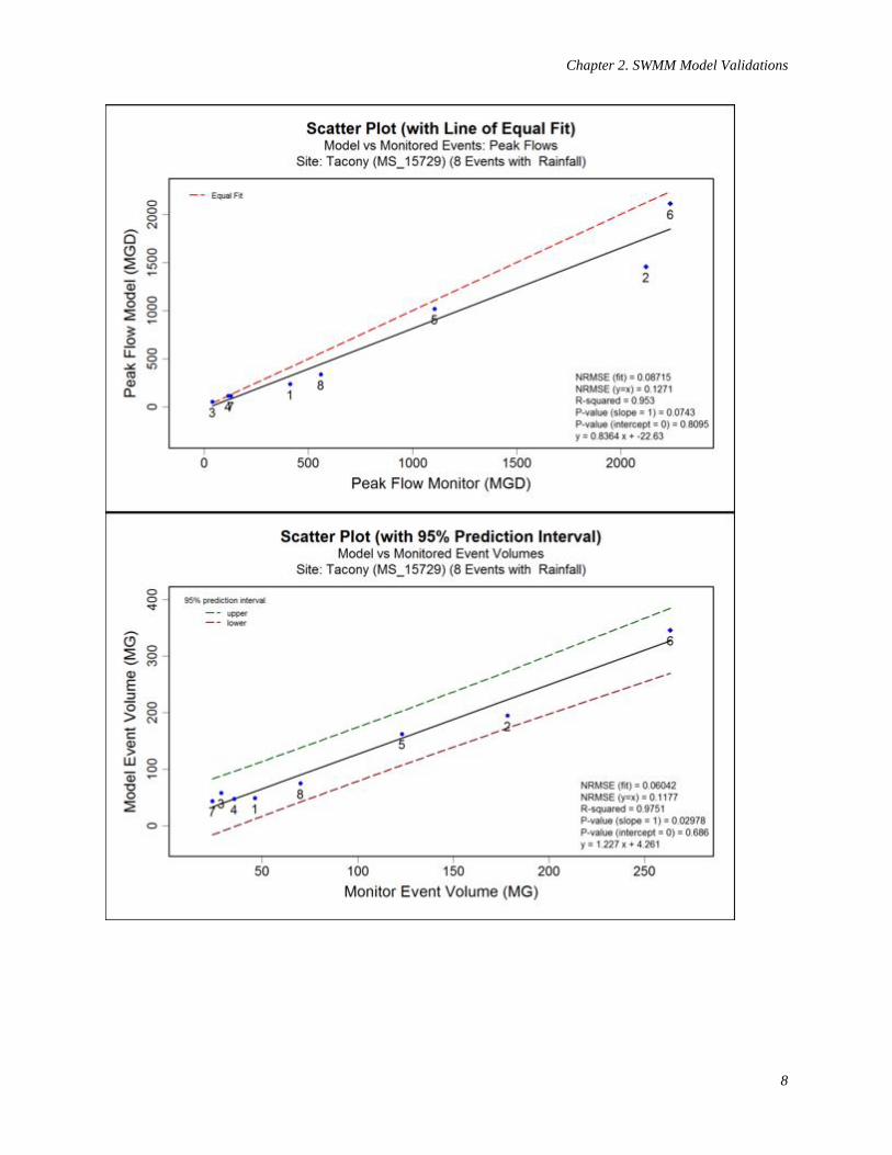
Chapter 2. SWMM Model Validations
8
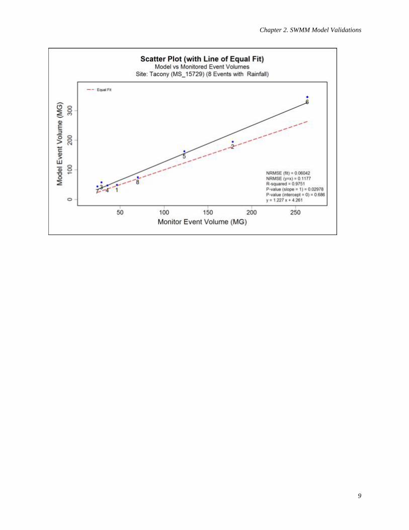
Chapter 2. SWMM Model Validations
9
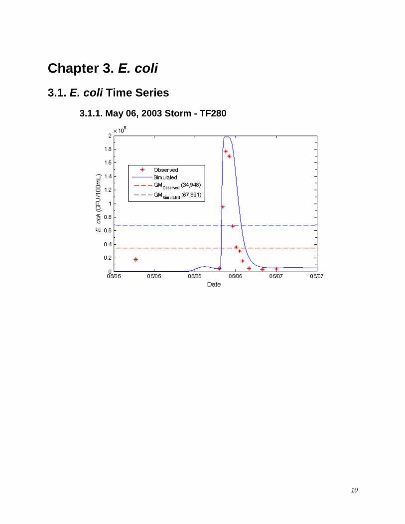
10
Chapter 3. E. coli
3.1. E. coli Time Series
3.1.1. May 06, 2003 Storm - TF280
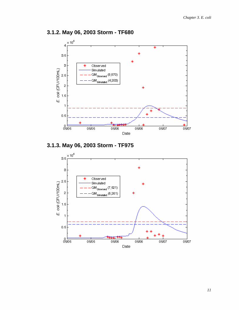
Chapter 3. E. coli
11
3.1.2. May 06, 2003 Storm - TF680
3.1.3. May 06, 2003 Storm - TF975
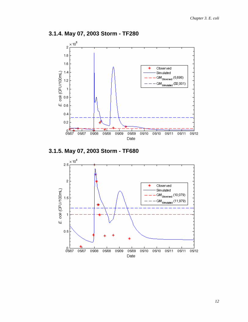
Chapter 3. E. coli
12
3.1.4. May 07, 2003 Storm - TF280
3.1.5. May 07, 2003 Storm - TF680
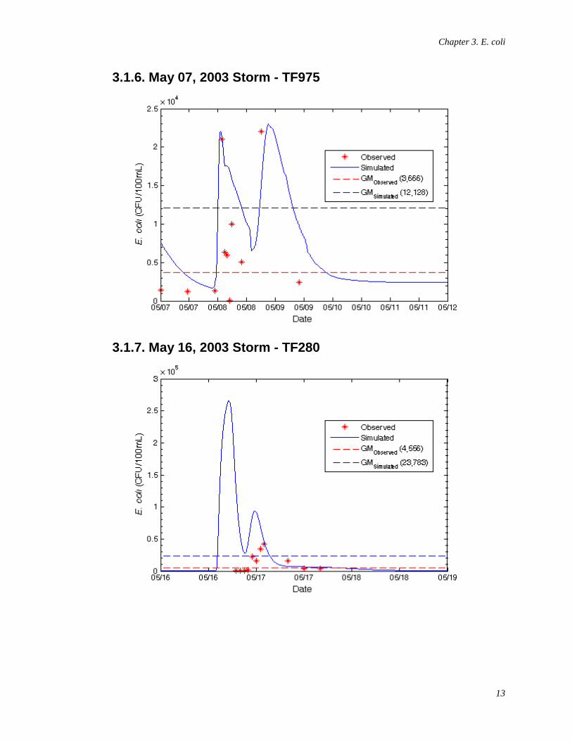
Chapter 3. E. coli
13
3.1.6. May 07, 2003 Storm - TF975
3.1.7. May 16, 2003 Storm - TF280
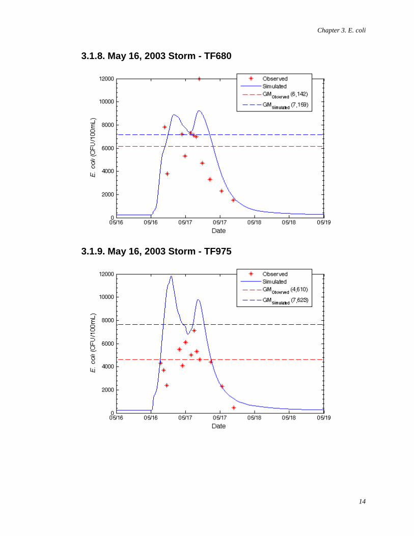
Chapter 3. E. coli
14
3.1.8. May 16, 2003 Storm - TF680
3.1.9. May 16, 2003 Storm - TF975
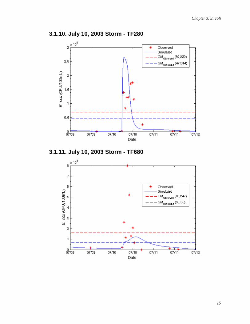
Chapter 3. E. coli
15
3.1.10. July 10, 2003 Storm - TF280
3.1.11. July 10, 2003 Storm - TF680
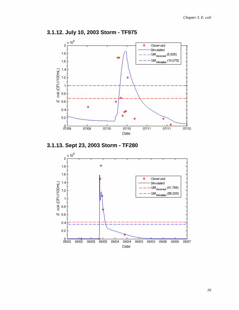
Chapter 3. E. coli
16
3.1.12. July 10, 2003 Storm - TF975
3.1.13. Sept 23, 2003 Storm - TF280
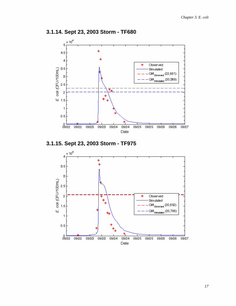
Chapter 3. E. coli
17
3.1.14. Sept 23, 2003 Storm - TF680
3.1.15. Sept 23, 2003 Storm - TF975
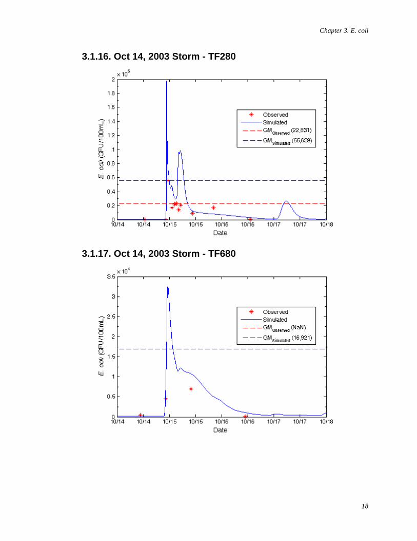
Chapter 3. E. coli
18
3.1.16. Oct 14, 2003 Storm - TF280
3.1.17. Oct 14, 2003 Storm - TF680
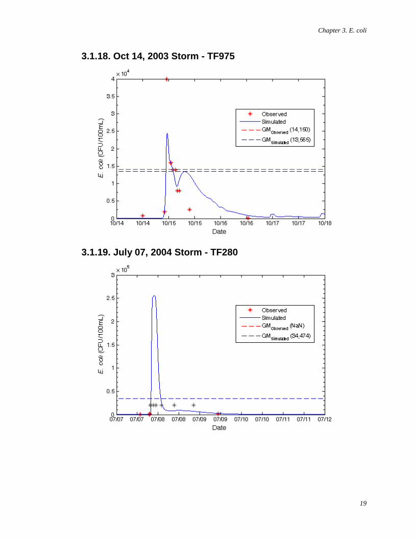
Chapter 3. E. coli
19
3.1.18. Oct 14, 2003 Storm - TF975
3.1.19. July 07, 2004 Storm - TF280
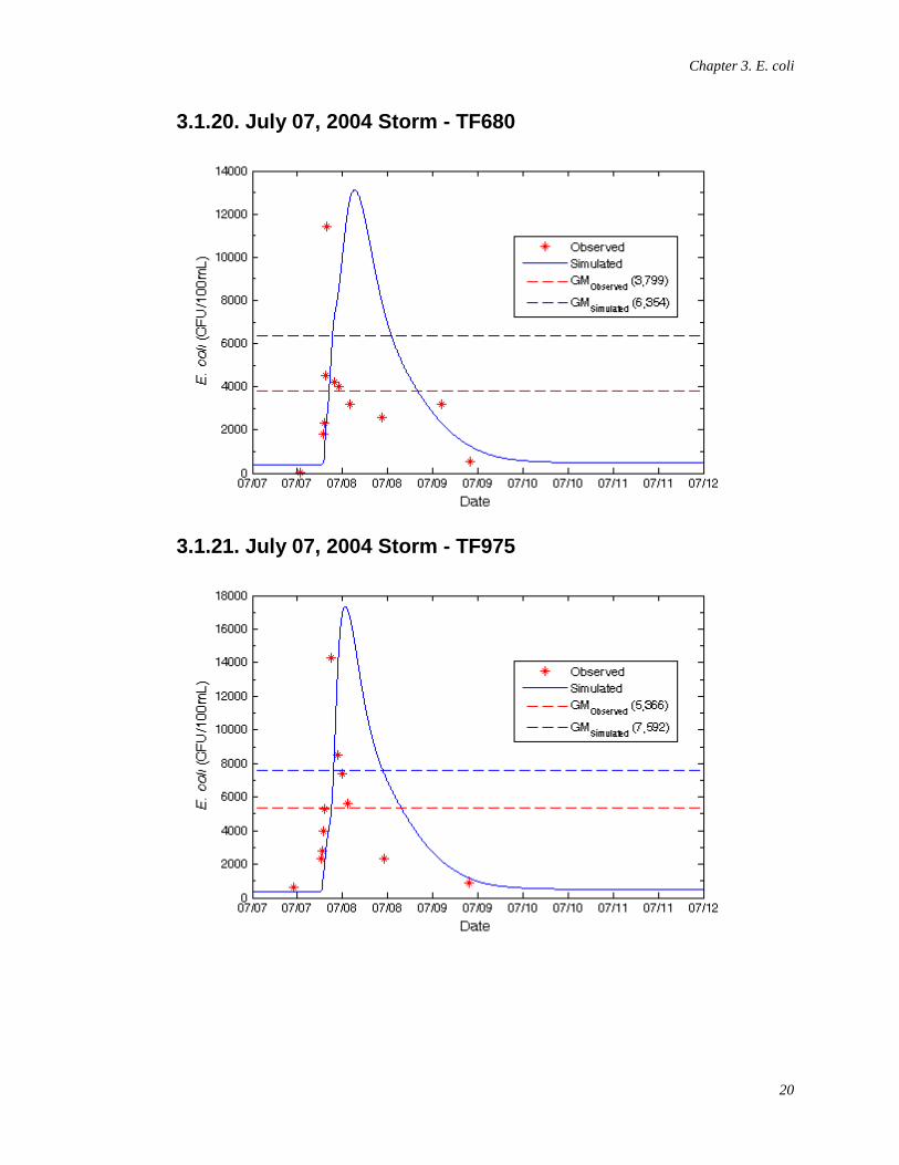
Chapter 3. E. coli
20
3.1.20. July 07, 2004 Storm - TF680
3.1.21. July 07, 2004 Storm - TF975
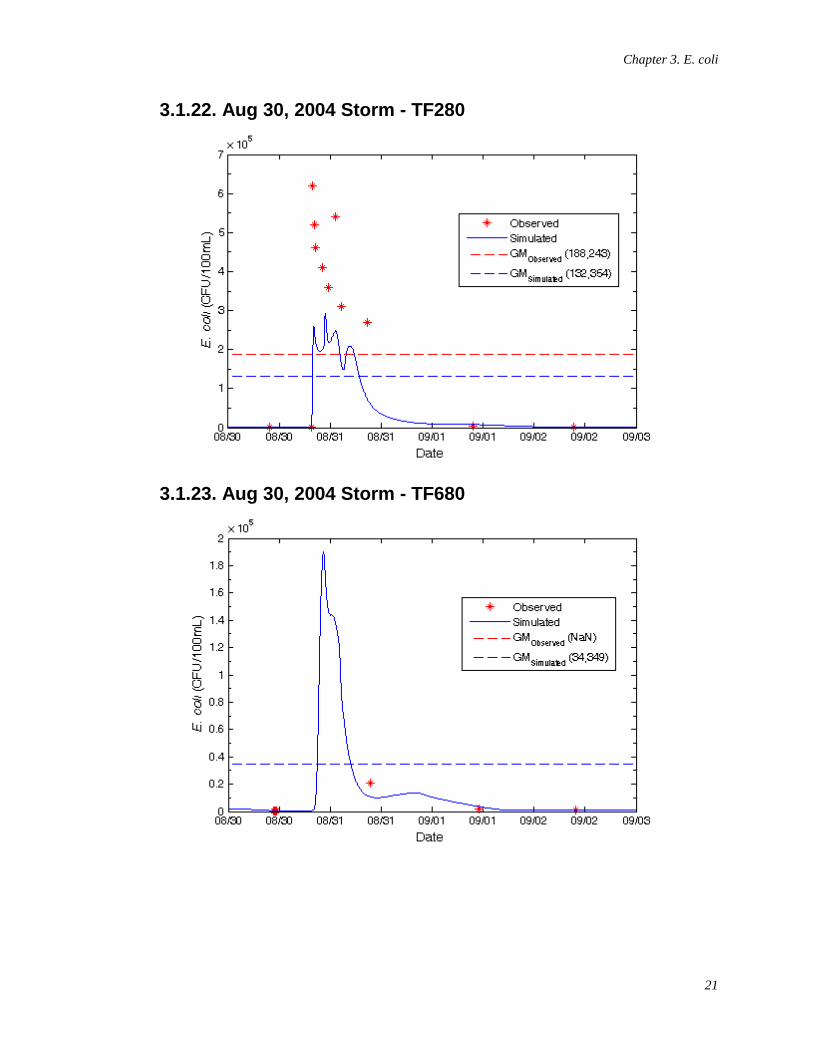
Chapter 3. E. coli
21
3.1.22. Aug 30, 2004 Storm - TF280
3.1.23. Aug 30, 2004 Storm - TF680
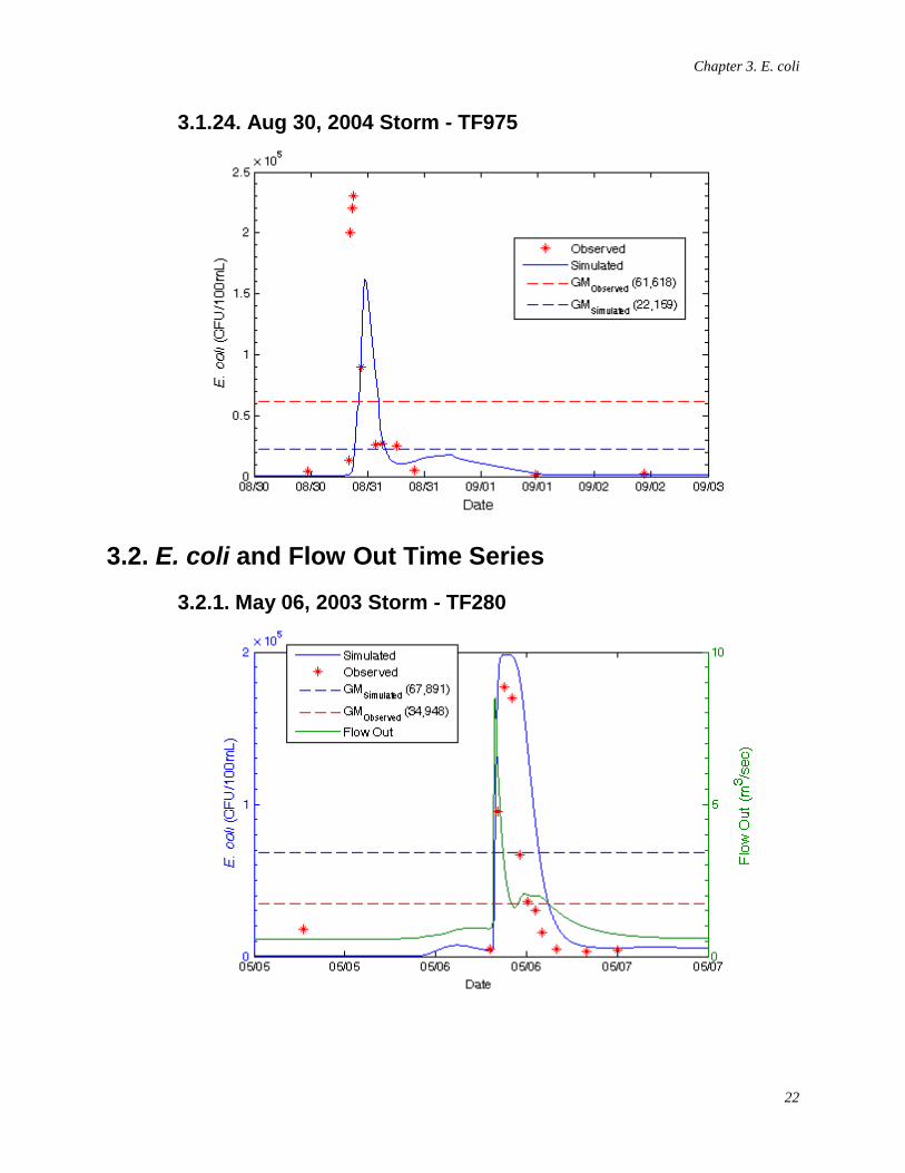
Chapter 3. E. coli
22
3.1.24. Aug 30, 2004 Storm - TF975
3.2. E. coli and Flow Out Time Series
3.2.1. May 06, 2003 Storm - TF280
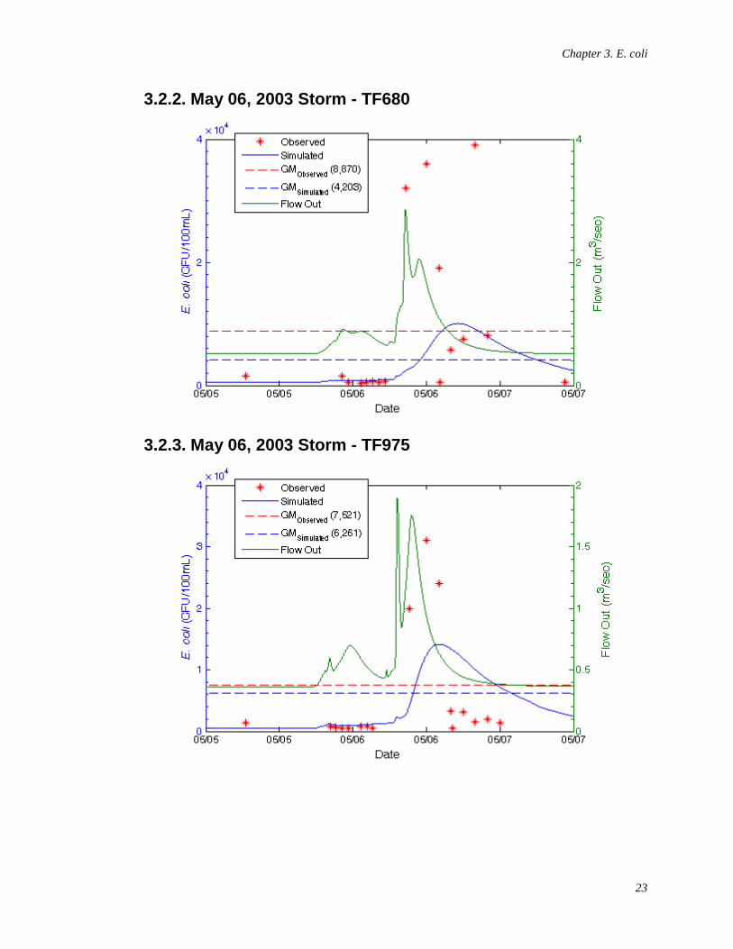
Chapter 3. E. coli
23
3.2.2. May 06, 2003 Storm - TF680
3.2.3. May 06, 2003 Storm - TF975
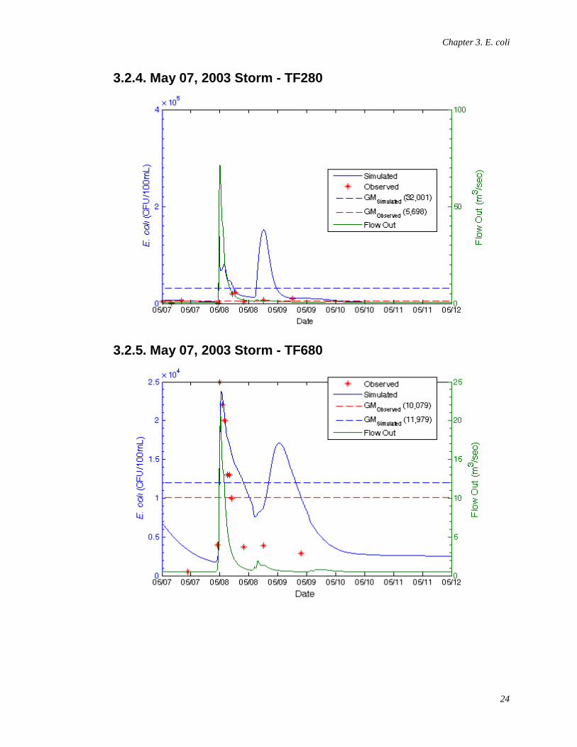
Chapter 3. E. coli
24
3.2.4. May 07, 2003 Storm - TF280
3.2.5. May 07, 2003 Storm - TF680
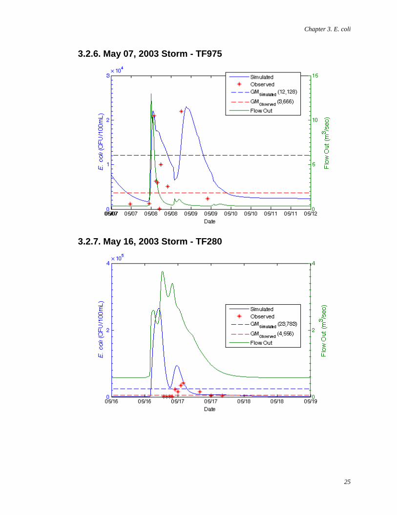
Chapter 3. E. coli
25
3.2.6. May 07, 2003 Storm - TF975
3.2.7. May 16, 2003 Storm - TF280
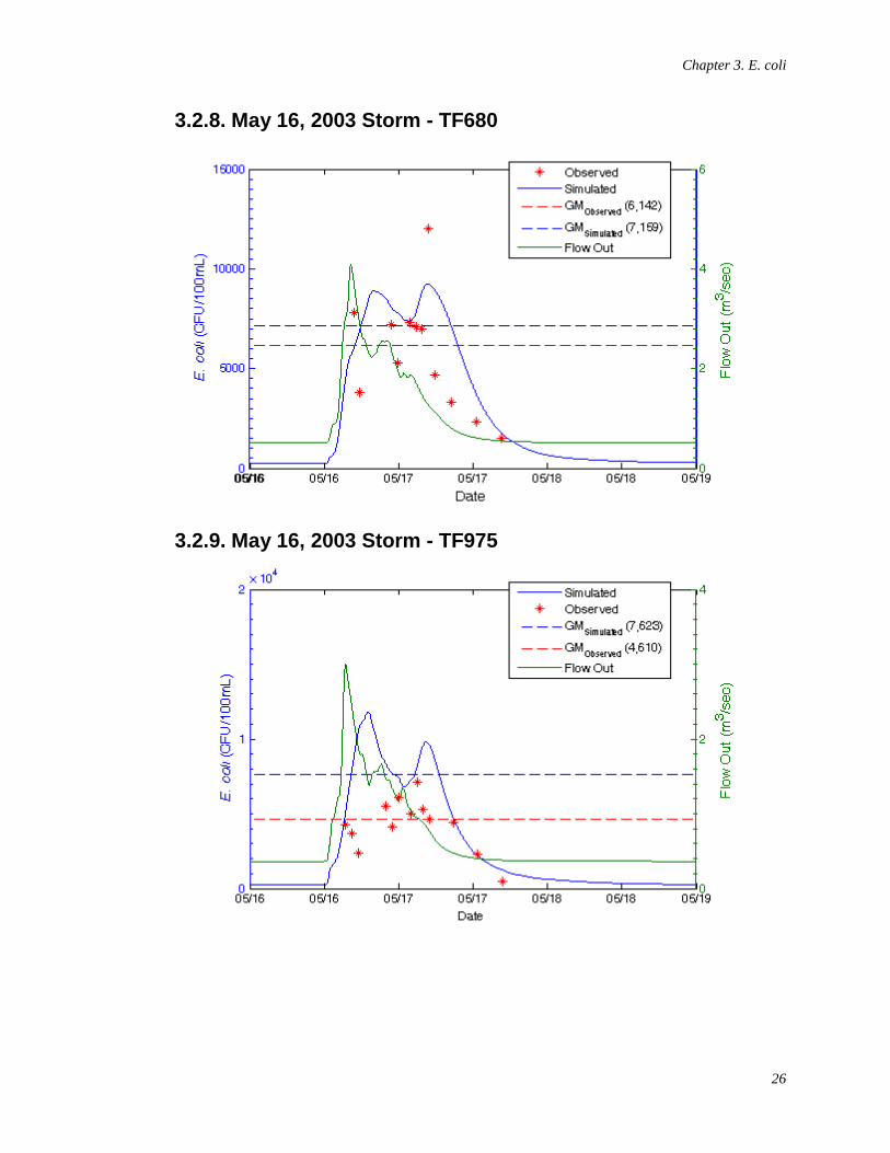
Chapter 3. E. coli
26
3.2.8. May 16, 2003 Storm - TF680
3.2.9. May 16, 2003 Storm - TF975
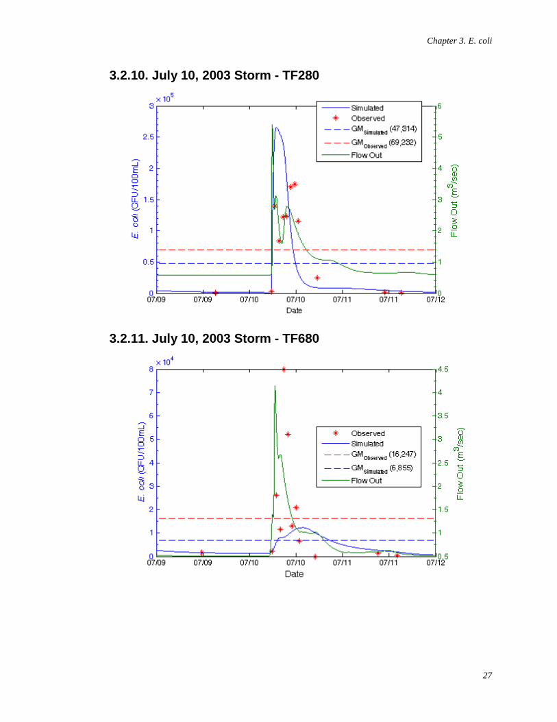
Chapter 3. E. coli
27
3.2.10. July 10, 2003 Storm - TF280
3.2.11. July 10, 2003 Storm - TF680
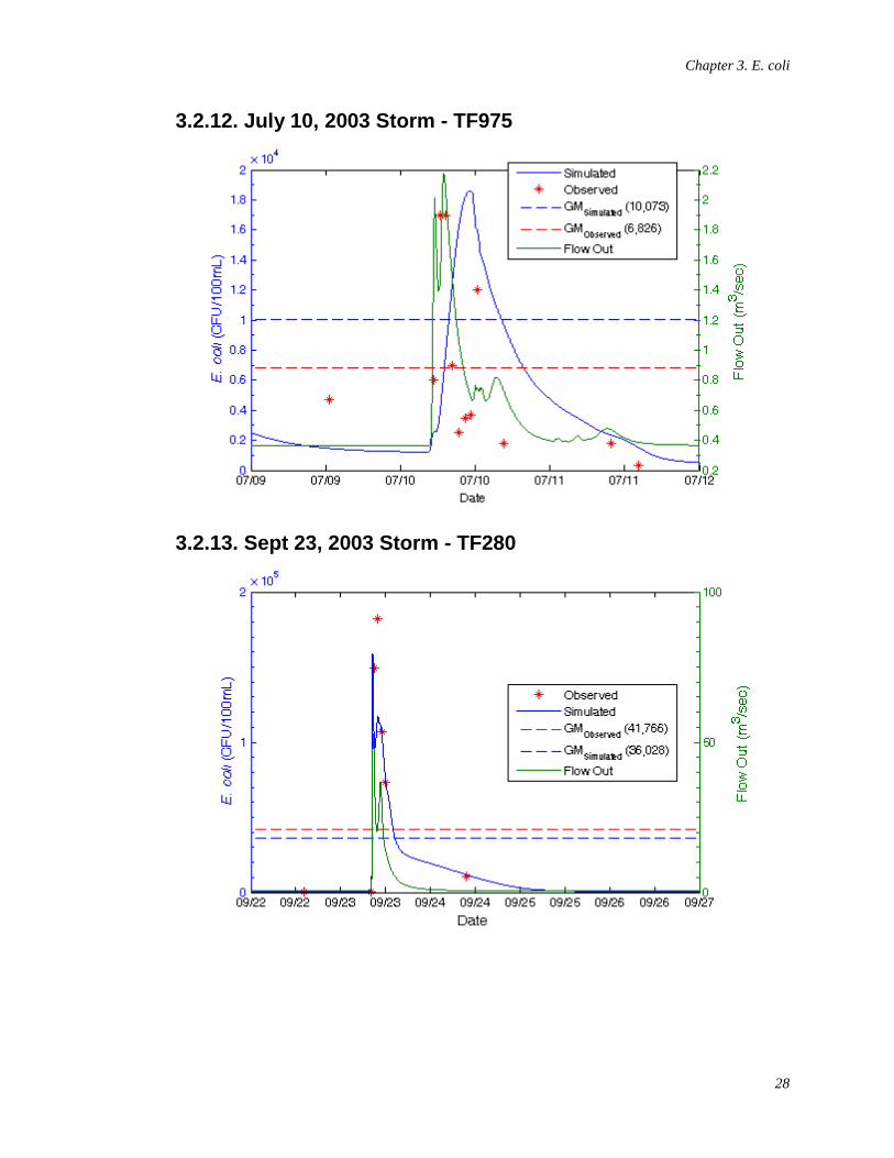
Chapter 3. E. coli
28
3.2.12. July 10, 2003 Storm - TF975
3.2.13. Sept 23, 2003 Storm - TF280
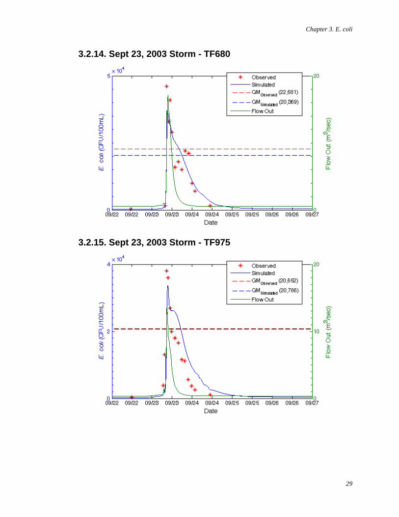
Chapter 3. E. coli
29
3.2.14. Sept 23, 2003 Storm - TF680
3.2.15. Sept 23, 2003 Storm - TF975
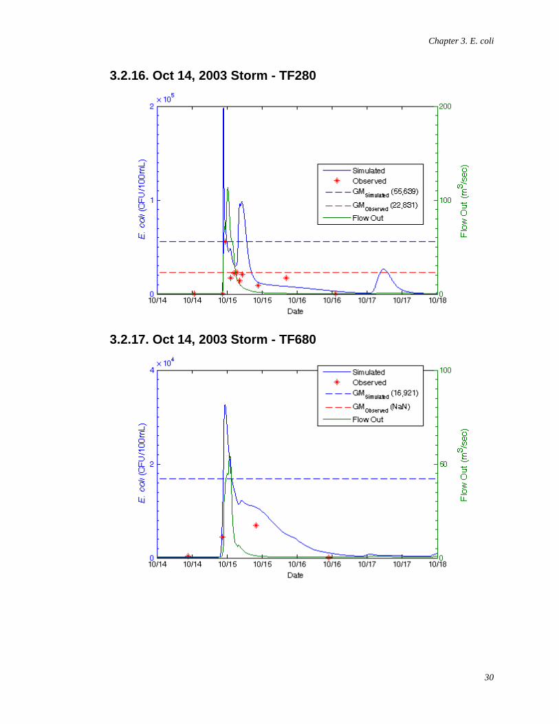
Chapter 3. E. coli
30
3.2.16. Oct 14, 2003 Storm - TF280
3.2.17. Oct 14, 2003 Storm - TF680
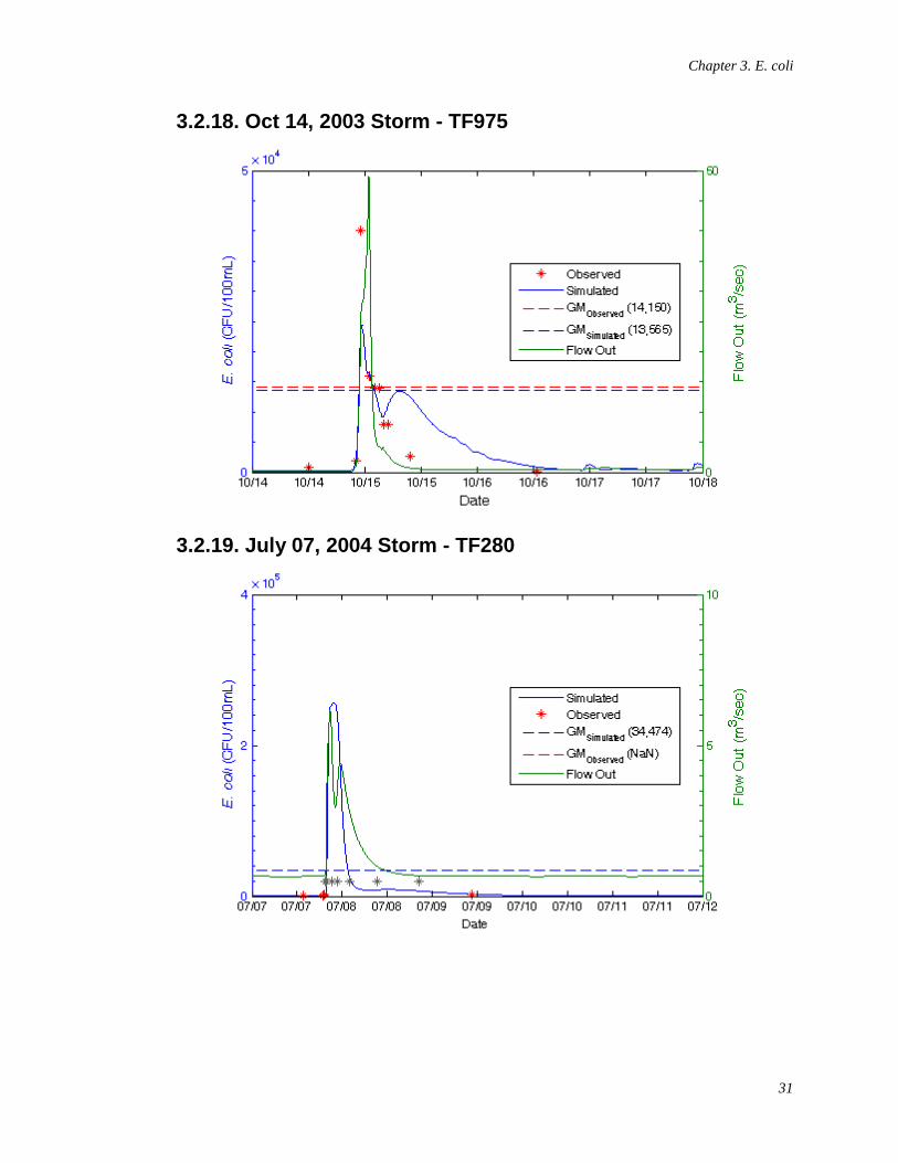
Chapter 3. E. coli
31
3.2.18. Oct 14, 2003 Storm - TF975
3.2.19. July 07, 2004 Storm - TF280
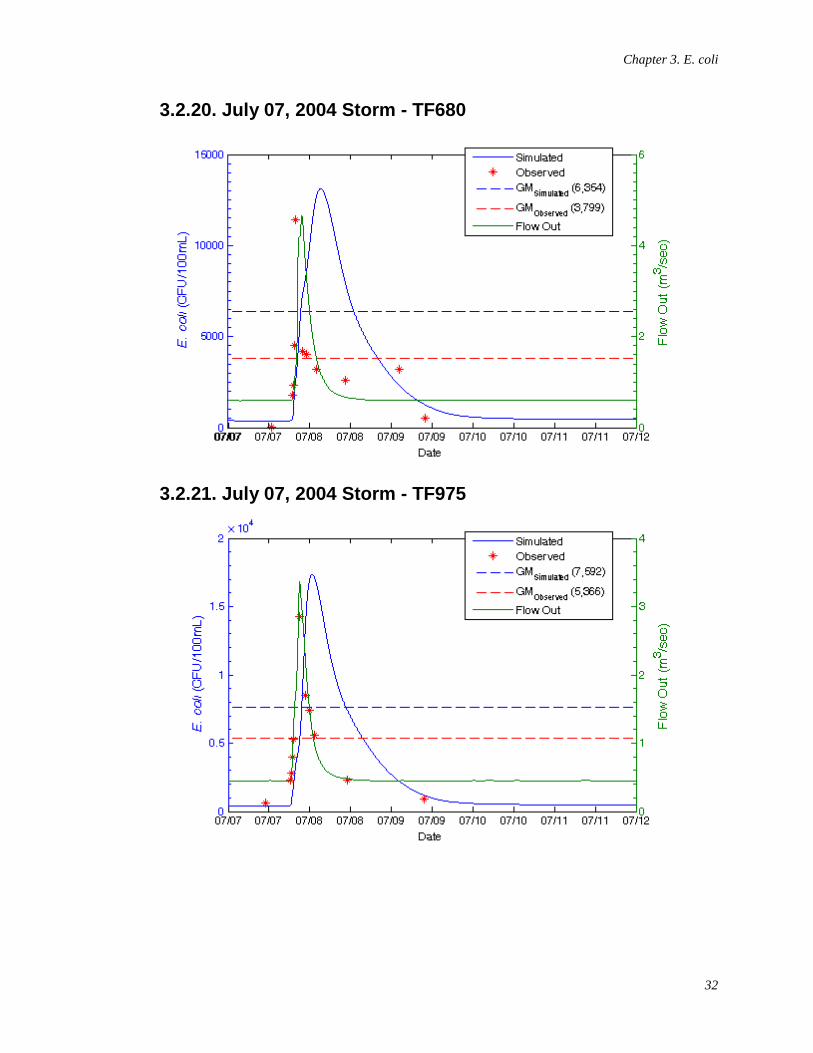
Chapter 3. E. coli
32
3.2.20. July 07, 2004 Storm - TF680
3.2.21. July 07, 2004 Storm - TF975
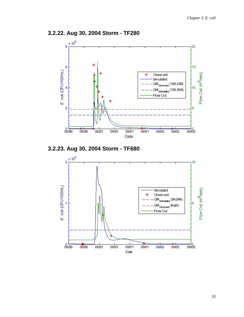
Chapter 3. E. coli
33
3.2.22. Aug 30, 2004 Storm - TF280
3.2.23. Aug 30, 2004 Storm - TF680
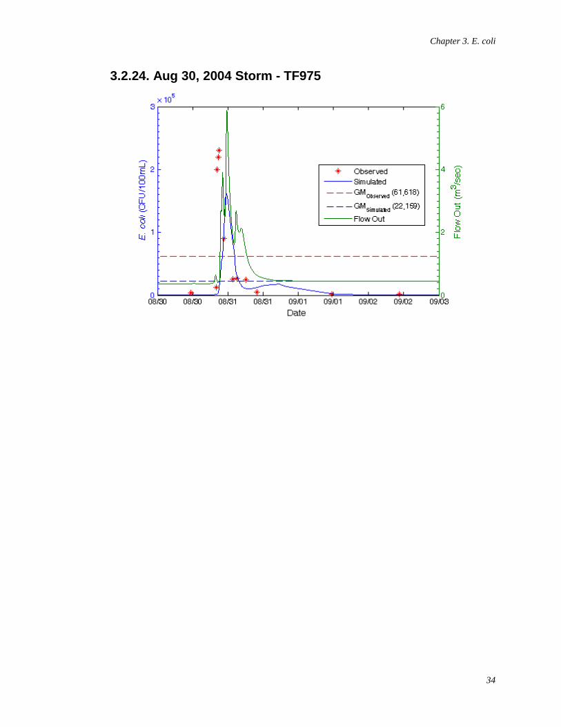
Chapter 3. E. coli
34
3.2.24. Aug 30, 2004 Storm - TF975
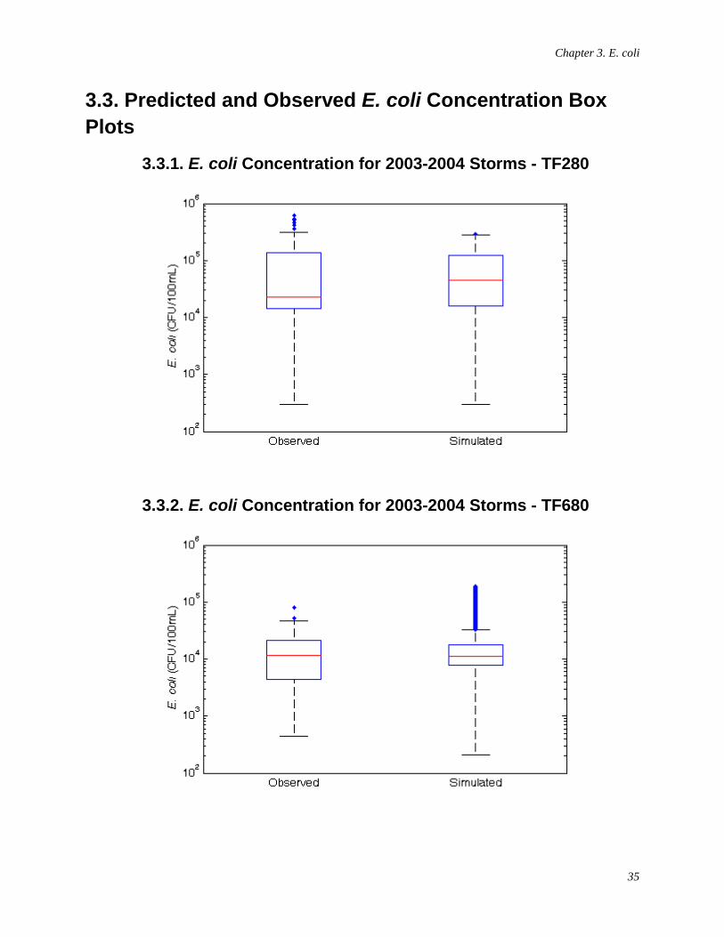
Chapter 3. E. coli
35
3.3. Predicted and Observed E. coli Concentration Box Plots
3.3.1. E. coli Concentration for 2003-2004 Storms - TF280
3.3.2. E. coli Concentration for 2003-2004 Storms - TF680
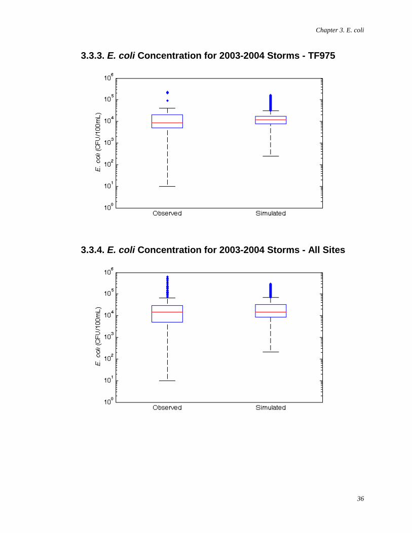
Chapter 3. E. coli
36
3.3.3. E. coli Concentration for 2003-2004 Storms - TF975
3.3.4. E. coli Concentration for 2003-2004 Storms - All Sites
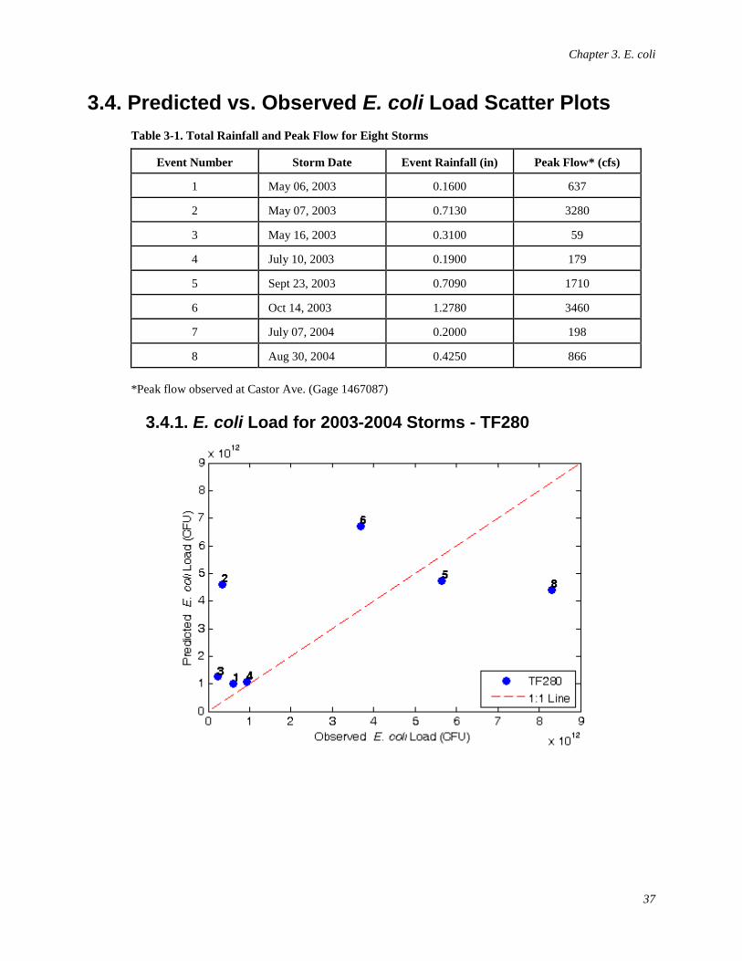
Chapter 3. E. coli
37
3.4. Predicted vs. Observed E. coli Load Scatter Plots Table 3-1. Total Rainfall and Peak Flow for Eight Storms
Event Number Storm Date Event Rainfall (in) Peak Flow* (cfs)
1 May 06, 2003 0.1600 637
2 May 07, 2003 0.7130 3280
3 May 16, 2003 0.3100 59
4 July 10, 2003 0.1900 179
5 Sept 23, 2003 0.7090 1710
6 Oct 14, 2003 1.2780 3460
7 July 07, 2004 0.2000 198
8 Aug 30, 2004 0.4250 866
*Peak flow observed at Castor Ave. (Gage 1467087)
3.4.1. E. coli Load for 2003-2004 Storms - TF280
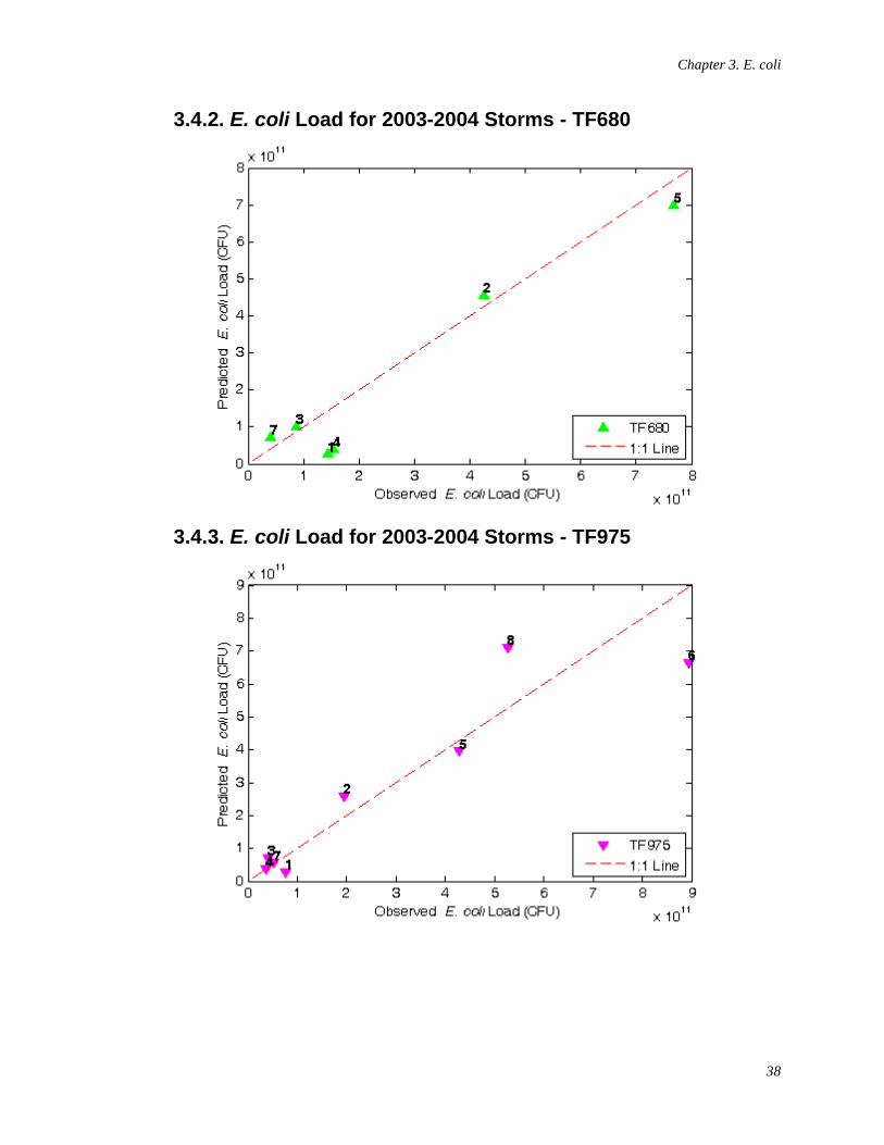
Chapter 3. E. coli
38
3.4.2. E. coli Load for 2003-2004 Storms - TF680
3.4.3. E. coli Load for 2003-2004 Storms - TF975
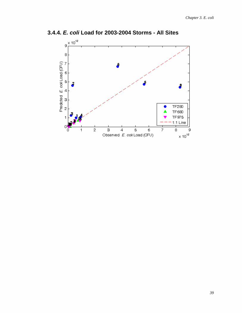
Chapter 3. E. coli
39
3.4.4. E. coli Load for 2003-2004 Storms - All Sites
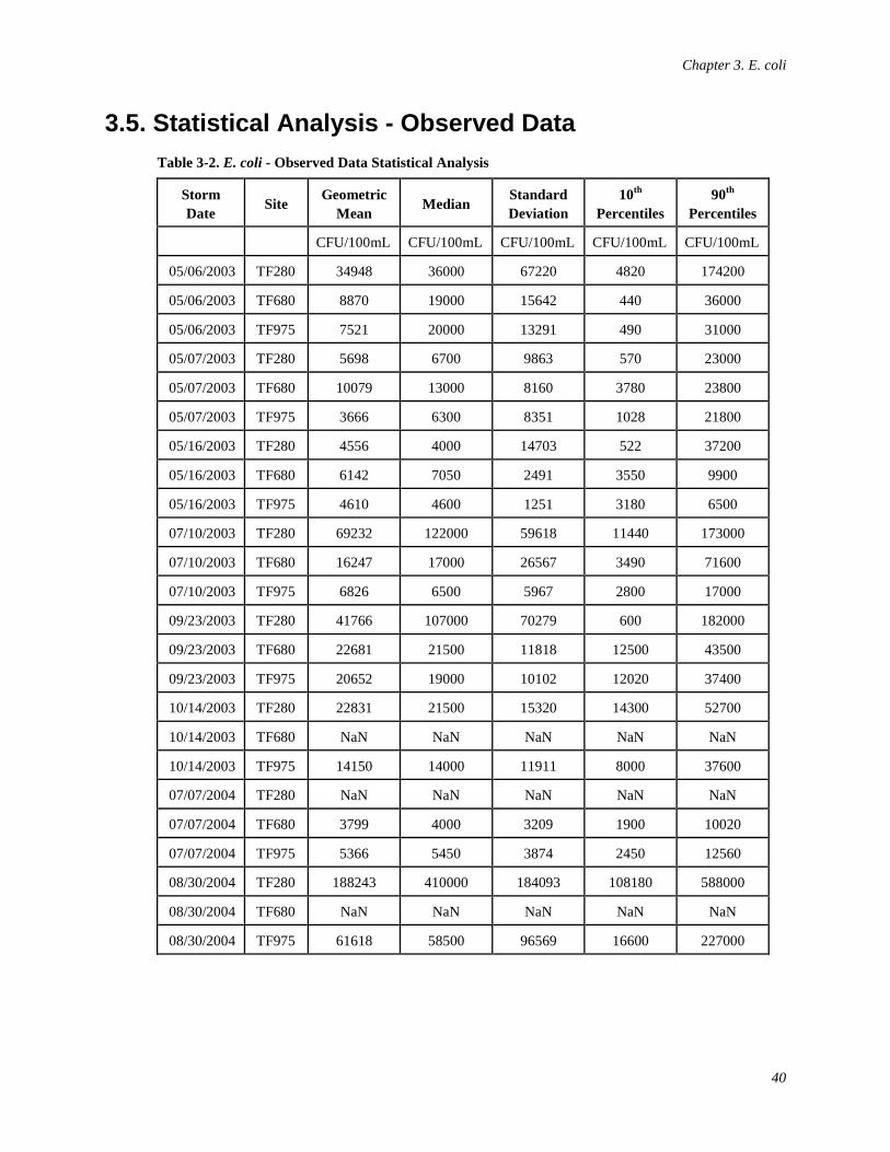
Chapter 3. E. coli
40
3.5. Statistical Analysis - Observed Data Table 3-2. E. coli - Observed Data Statistical Analysis
Storm Date Site Geometric
Mean Median Standard Deviation
10th Percentiles
90th Percentiles
CFU/100mL CFU/100mL CFU/100mL CFU/100mL CFU/100mL
05/06/2003 TF280 34948 36000 67220 4820 174200
05/06/2003 TF680 8870 19000 15642 440 36000
05/06/2003 TF975 7521 20000 13291 490 31000
05/07/2003 TF280 5698 6700 9863 570 23000
05/07/2003 TF680 10079 13000 8160 3780 23800
05/07/2003 TF975 3666 6300 8351 1028 21800
05/16/2003 TF280 4556 4000 14703 522 37200
05/16/2003 TF680 6142 7050 2491 3550 9900
05/16/2003 TF975 4610 4600 1251 3180 6500
07/10/2003 TF280 69232 122000 59618 11440 173000
07/10/2003 TF680 16247 17000 26567 3490 71600
07/10/2003 TF975 6826 6500 5967 2800 17000
09/23/2003 TF280 41766 107000 70279 600 182000
09/23/2003 TF680 22681 21500 11818 12500 43500
09/23/2003 TF975 20652 19000 10102 12020 37400
10/14/2003 TF280 22831 21500 15320 14300 52700
10/14/2003 TF680 NaN NaN NaN NaN NaN
10/14/2003 TF975 14150 14000 11911 8000 37600
07/07/2004 TF280 NaN NaN NaN NaN NaN
07/07/2004 TF680 3799 4000 3209 1900 10020
07/07/2004 TF975 5366 5450 3874 2450 12560
08/30/2004 TF280 188243 410000 184093 108180 588000
08/30/2004 TF680 NaN NaN NaN NaN NaN
08/30/2004 TF975 61618 58500 96569 16600 227000

Chapter 3. E. coli
41
3.6. Statistical Analysis - Simulated Data Table 3-3. E. coli - Simulated Data Statistical Analysis
Storm Date Site Geometric
Mean Median Standard Deviation
10th Percentiles
90th Percentiles
CFU/100mL CFU/100mL CFU/100mL CFU/100mL CFU/100mL
05/06/2003 TF280 67891 100519 73654 15362 198202
05/06/2003 TF680 4203 4831 3164 1494 9783
05/06/2003 TF975 6261 9996 5164 1378 14061
05/07/2003 TF280 32001 28297 40279 12867 112286
05/07/2003 TF680 11979 12405 4806 7870 20386
05/07/2003 TF975 12128 12944 4560 6932 19122
05/16/2003 TF280 23783 18413 72931 6487 185570
05/16/2003 TF680 7159 7881 1709 5300 8948
05/16/2003 TF975 7623 7932 2167 5026 10980
07/10/2003 TF280 47314 43964 98394 9255 255578
07/10/2003 TF680 6855 8230 3260 1996 11750
07/10/2003 TF975 10073 14411 5812 2591 18461
09/23/2003 TF280 36028 27226 35084 20325 108739
09/23/2003 TF680 20369 22145 7193 12433 31942
09/23/2003 TF975 20786 25552 7211 13165 29904
10/14/2003 TF280 55639 48225 34044 30589 97280
10/14/2003 TF680 16921 15183 6914 11709 30323
10/14/2003 TF975 13565 13079 4593 9425 22234
07/07/2004 TF280 34474 23669 97089 8404 253108
07/07/2004 TF680 6354 10083 4368 945 13028
07/07/2004 TF975 7592 14288 6221 1476 17214
08/30/2004 TF280 132354 196391 69406 63757 243473
08/30/2004 TF680 34349 47437 61570 3447 155697
08/30/2004 TF975 22159 22997 50871 1725 138842
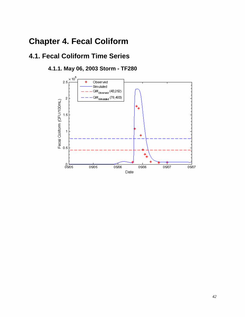
42
Chapter 4. Fecal Coliform
4.1. Fecal Coliform Time Series
4.1.1. May 06, 2003 Storm - TF280
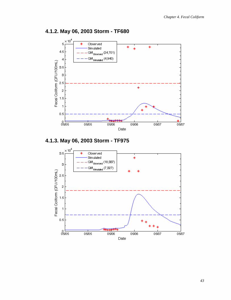
Chapter 4. Fecal Coliform
43
4.1.2. May 06, 2003 Storm - TF680
4.1.3. May 06, 2003 Storm - TF975
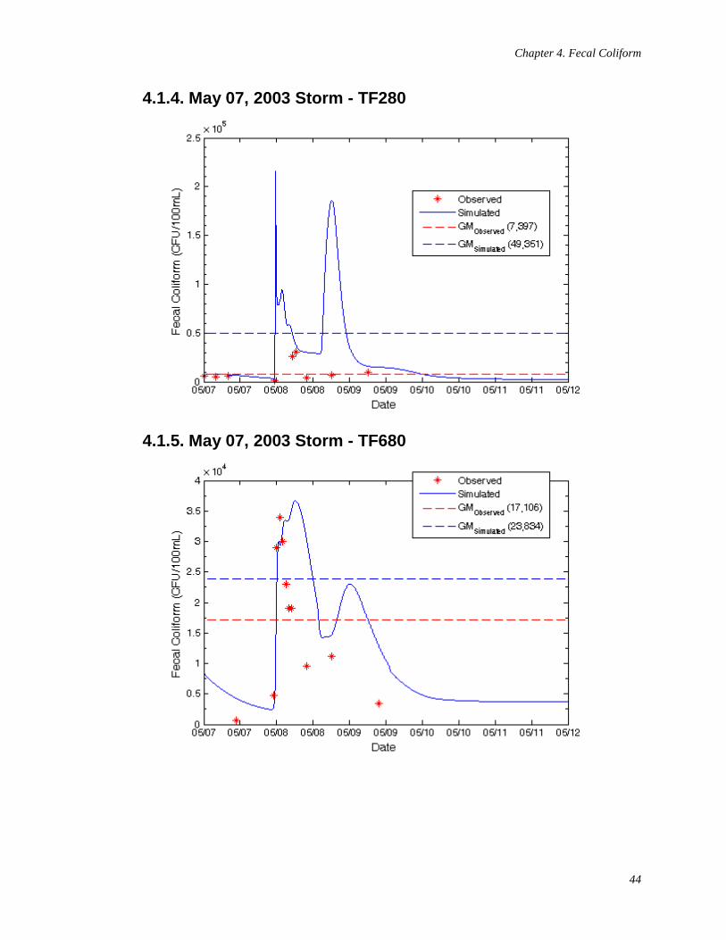
Chapter 4. Fecal Coliform
44
4.1.4. May 07, 2003 Storm - TF280
4.1.5. May 07, 2003 Storm - TF680
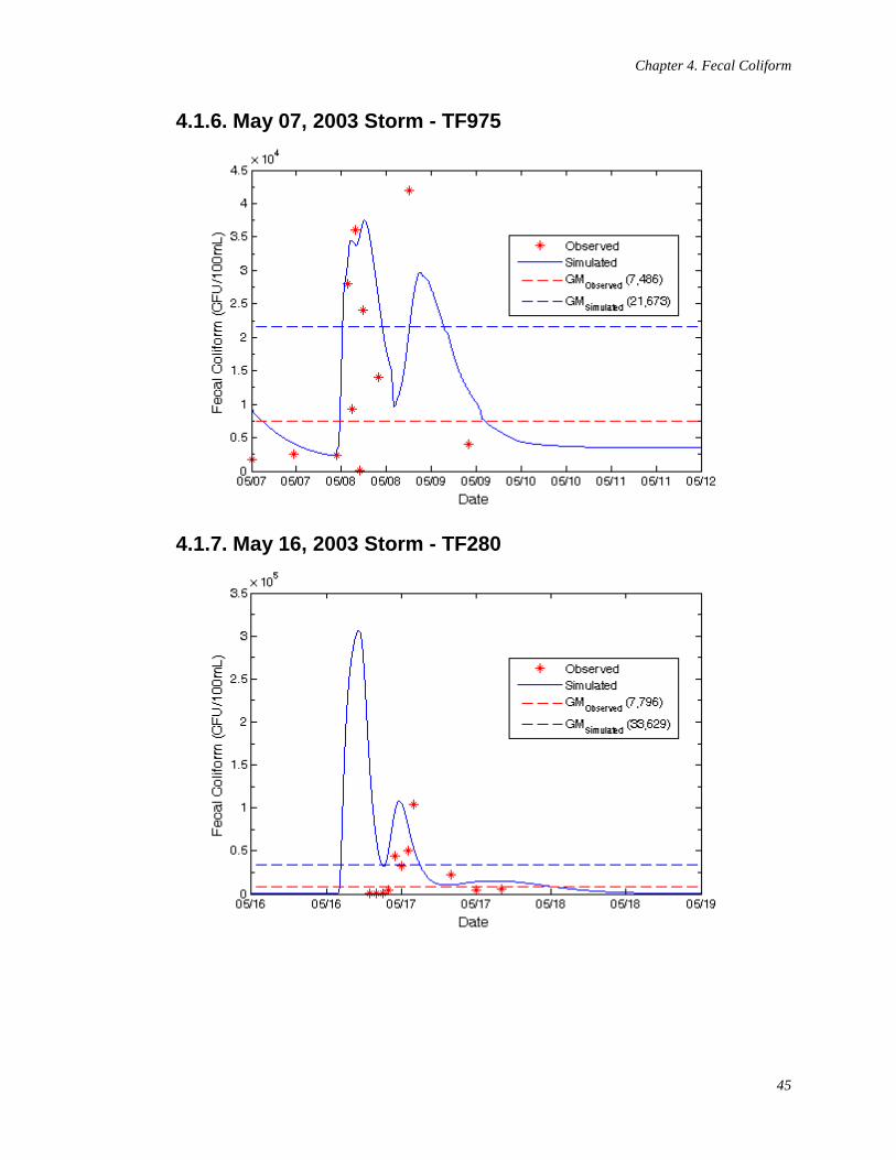
Chapter 4. Fecal Coliform
45
4.1.6. May 07, 2003 Storm - TF975
4.1.7. May 16, 2003 Storm - TF280
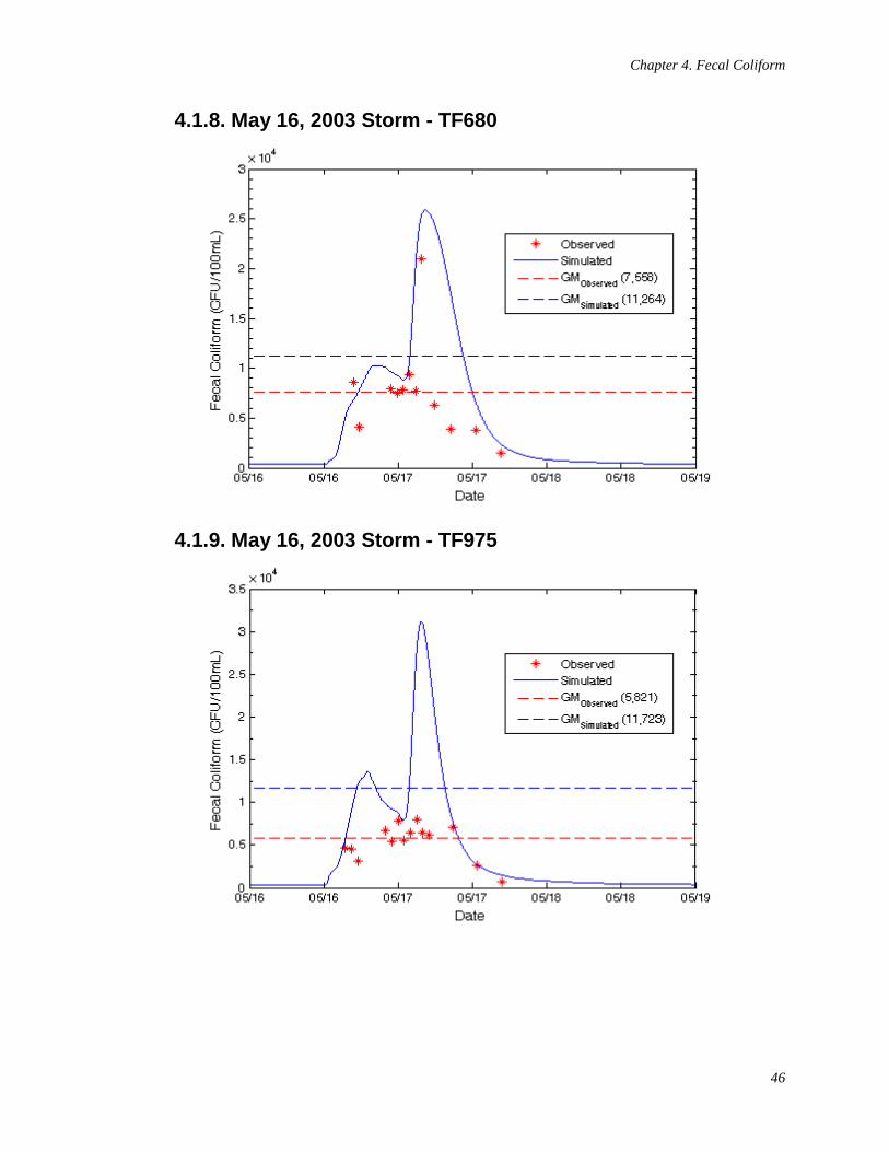
Chapter 4. Fecal Coliform
46
4.1.8. May 16, 2003 Storm - TF680
4.1.9. May 16, 2003 Storm - TF975
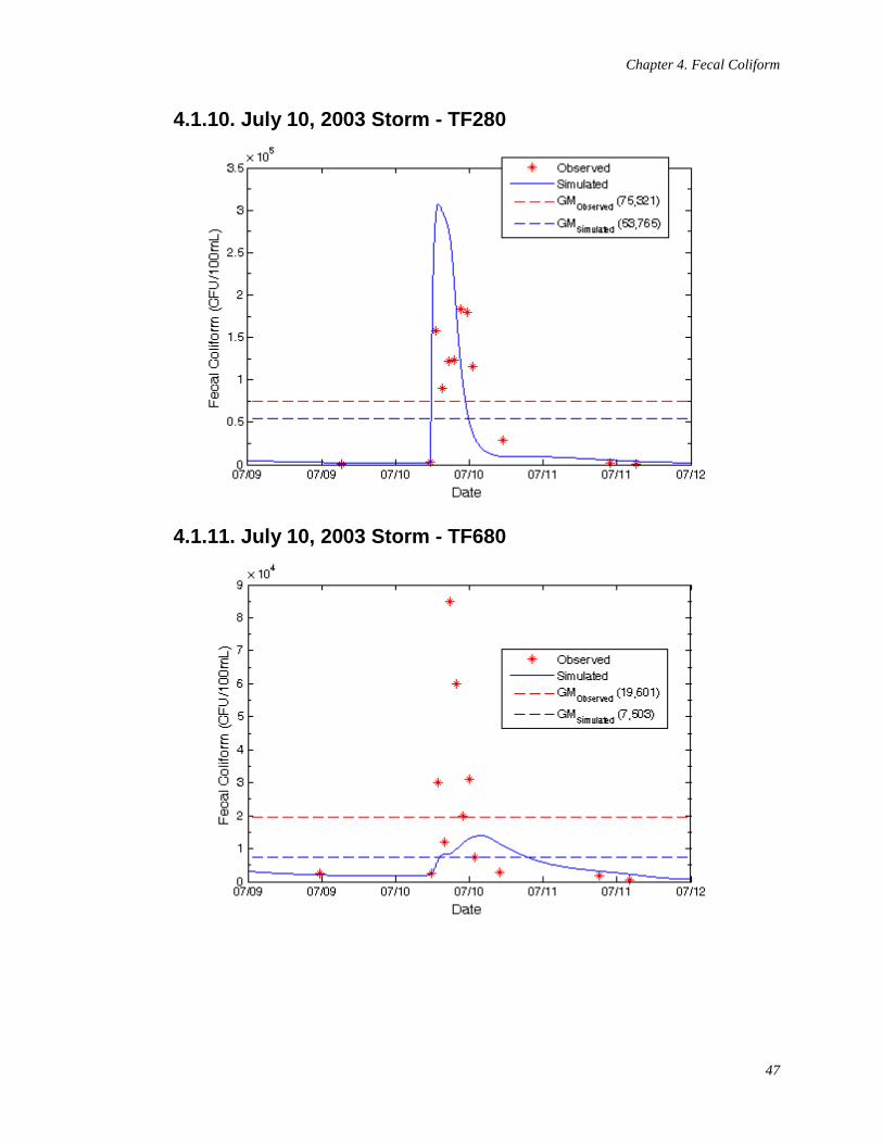
Chapter 4. Fecal Coliform
47
4.1.10. July 10, 2003 Storm - TF280
4.1.11. July 10, 2003 Storm - TF680
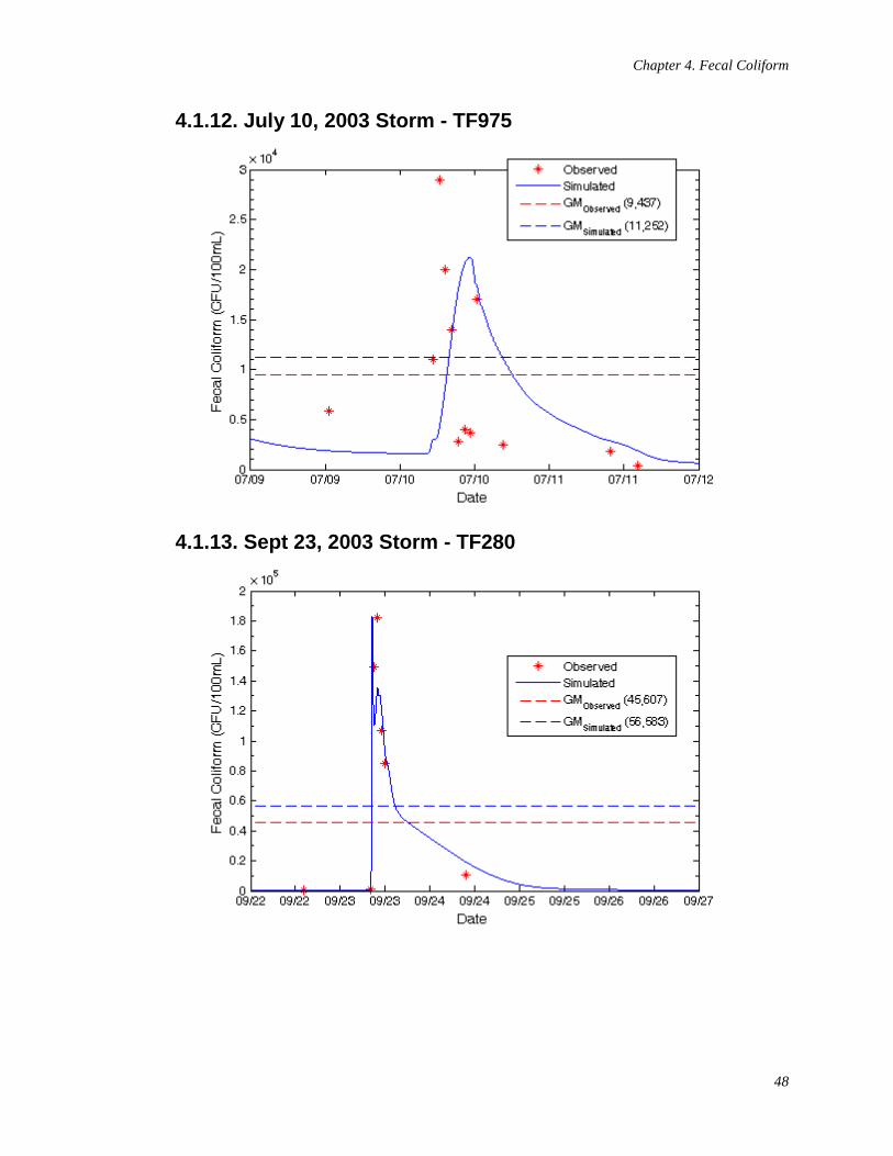
Chapter 4. Fecal Coliform
48
4.1.12. July 10, 2003 Storm - TF975
4.1.13. Sept 23, 2003 Storm - TF280
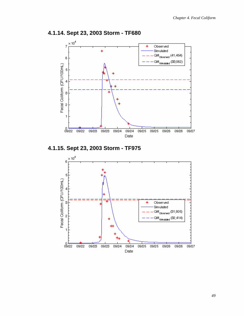
Chapter 4. Fecal Coliform
49
4.1.14. Sept 23, 2003 Storm - TF680
4.1.15. Sept 23, 2003 Storm - TF975
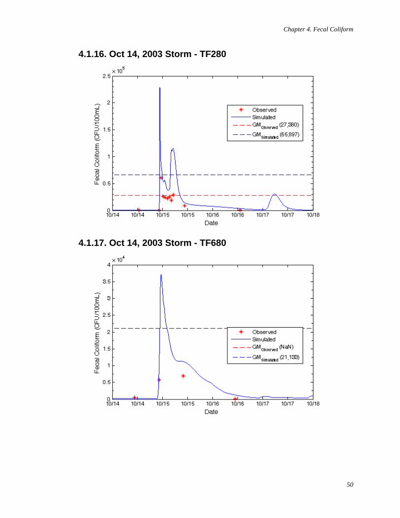
Chapter 4. Fecal Coliform
50
4.1.16. Oct 14, 2003 Storm - TF280
4.1.17. Oct 14, 2003 Storm - TF680
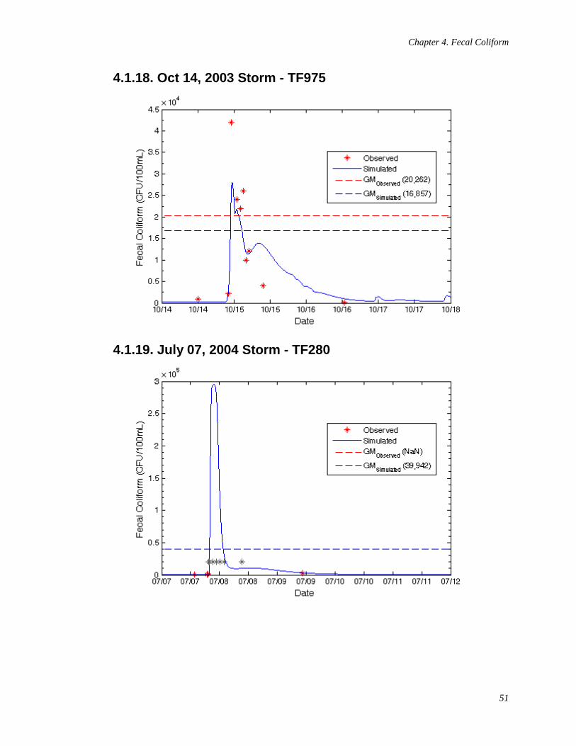
Chapter 4. Fecal Coliform
51
4.1.18. Oct 14, 2003 Storm - TF975
4.1.19. July 07, 2004 Storm - TF280
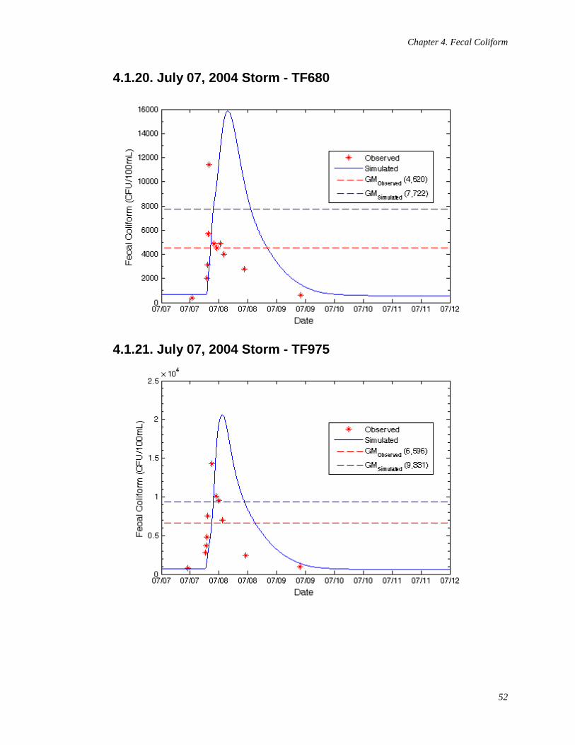
Chapter 4. Fecal Coliform
52
4.1.20. July 07, 2004 Storm - TF680
4.1.21. July 07, 2004 Storm - TF975
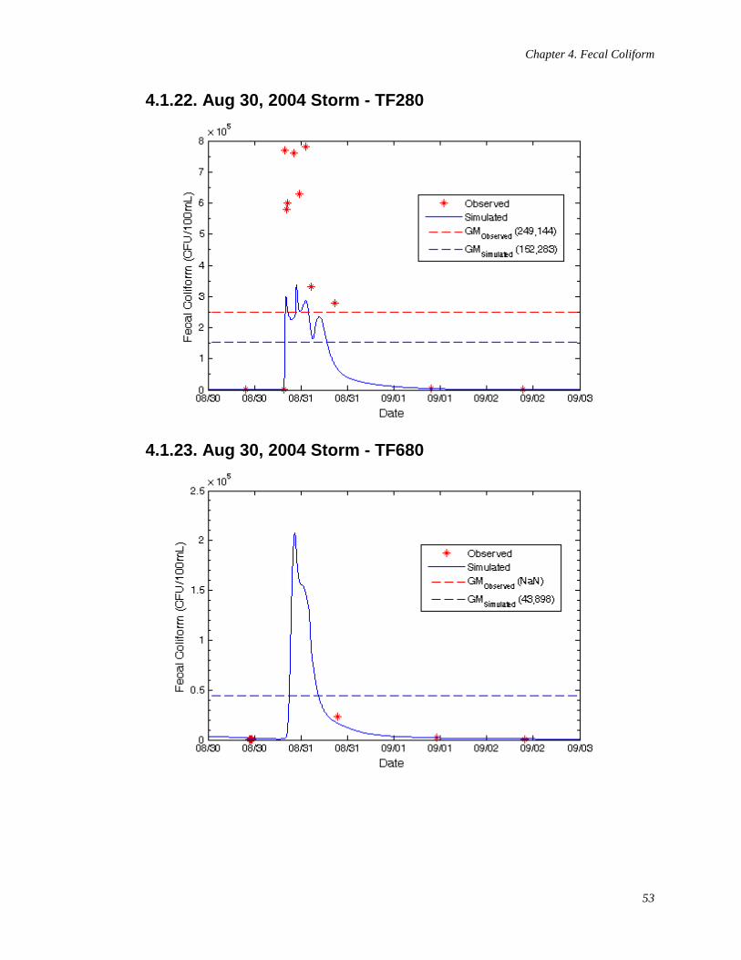
Chapter 4. Fecal Coliform
53
4.1.22. Aug 30, 2004 Storm - TF280
4.1.23. Aug 30, 2004 Storm - TF680
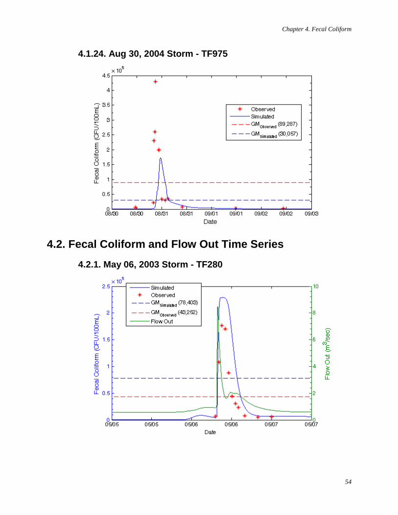
Chapter 4. Fecal Coliform
54
4.1.24. Aug 30, 2004 Storm - TF975
4.2. Fecal Coliform and Flow Out Time Series
4.2.1. May 06, 2003 Storm - TF280
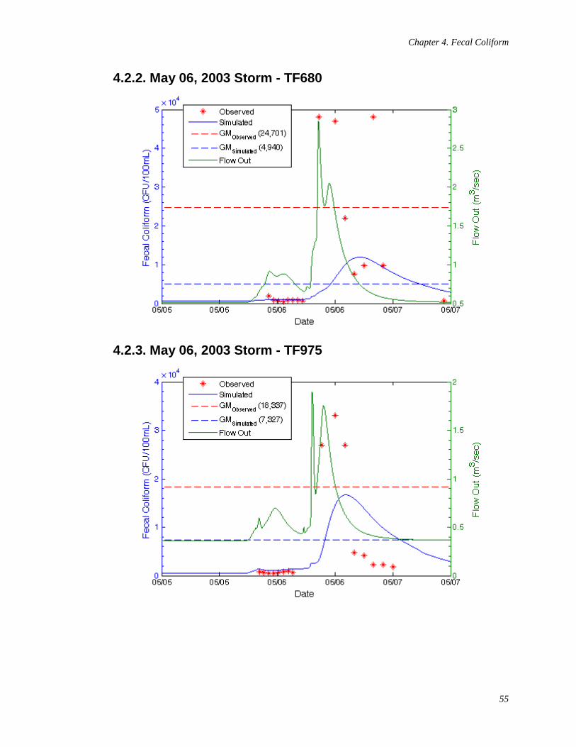
Chapter 4. Fecal Coliform
55
4.2.2. May 06, 2003 Storm - TF680
4.2.3. May 06, 2003 Storm - TF975
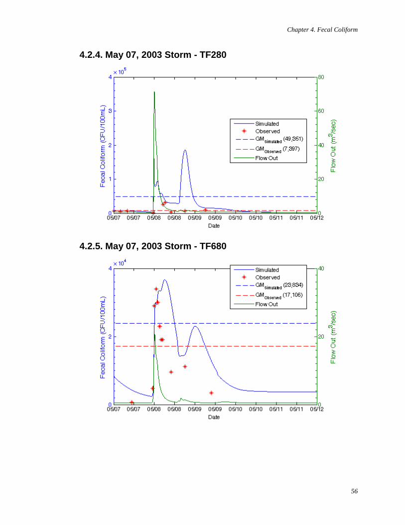
Chapter 4. Fecal Coliform
56
4.2.4. May 07, 2003 Storm - TF280
4.2.5. May 07, 2003 Storm - TF680
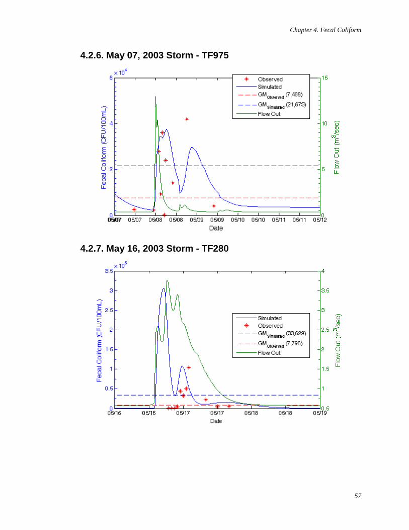
Chapter 4. Fecal Coliform
57
4.2.6. May 07, 2003 Storm - TF975
4.2.7. May 16, 2003 Storm - TF280
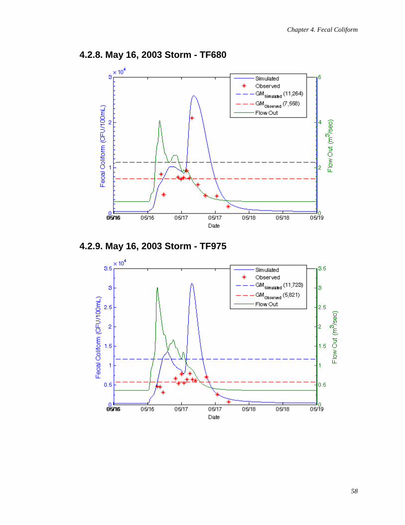
Chapter 4. Fecal Coliform
58
4.2.8. May 16, 2003 Storm - TF680
4.2.9. May 16, 2003 Storm - TF975
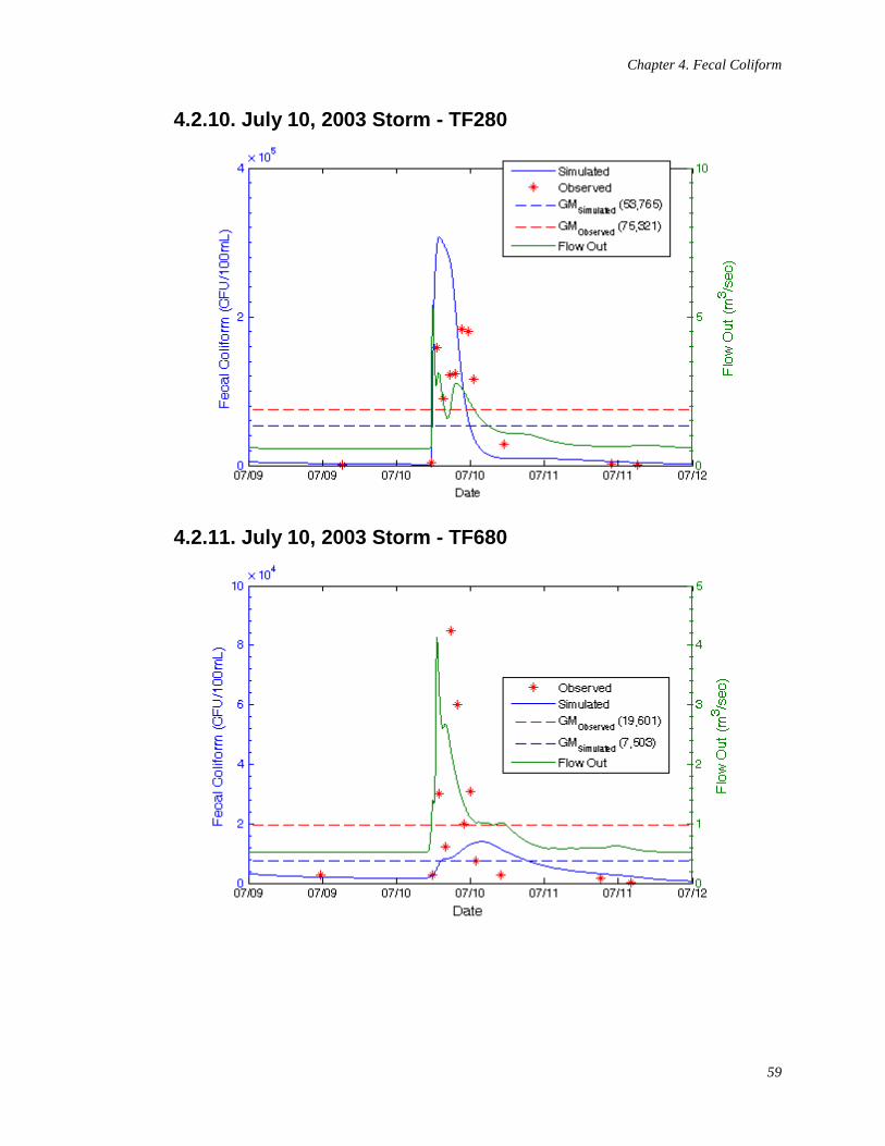
Chapter 4. Fecal Coliform
59
4.2.10. July 10, 2003 Storm - TF280
4.2.11. July 10, 2003 Storm - TF680
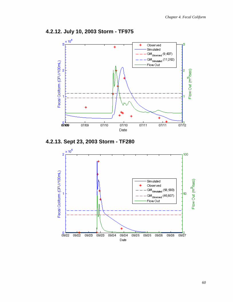
Chapter 4. Fecal Coliform
60
4.2.12. July 10, 2003 Storm - TF975
4.2.13. Sept 23, 2003 Storm - TF280
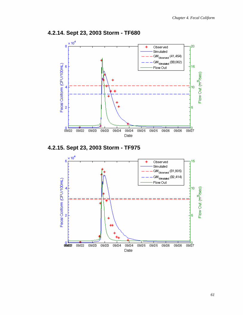
Chapter 4. Fecal Coliform
61
4.2.14. Sept 23, 2003 Storm - TF680
4.2.15. Sept 23, 2003 Storm - TF975
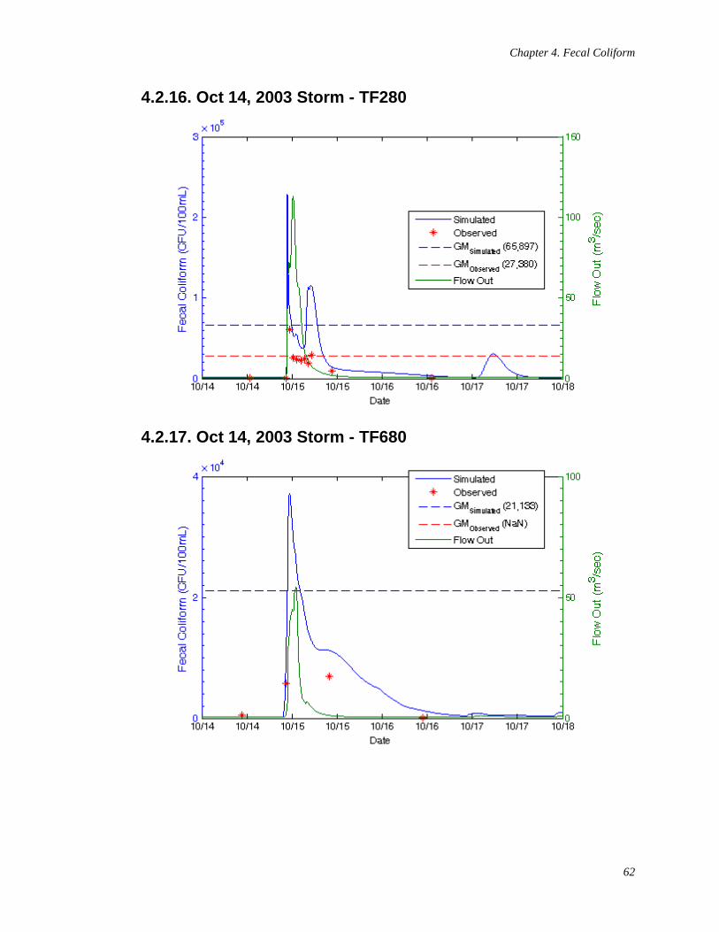
Chapter 4. Fecal Coliform
62
4.2.16. Oct 14, 2003 Storm - TF280
4.2.17. Oct 14, 2003 Storm - TF680
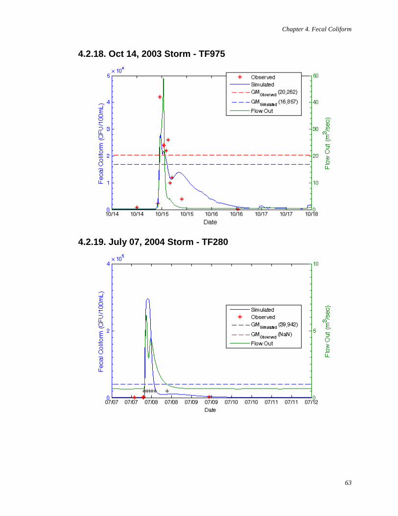
Chapter 4. Fecal Coliform
63
4.2.18. Oct 14, 2003 Storm - TF975
4.2.19. July 07, 2004 Storm - TF280
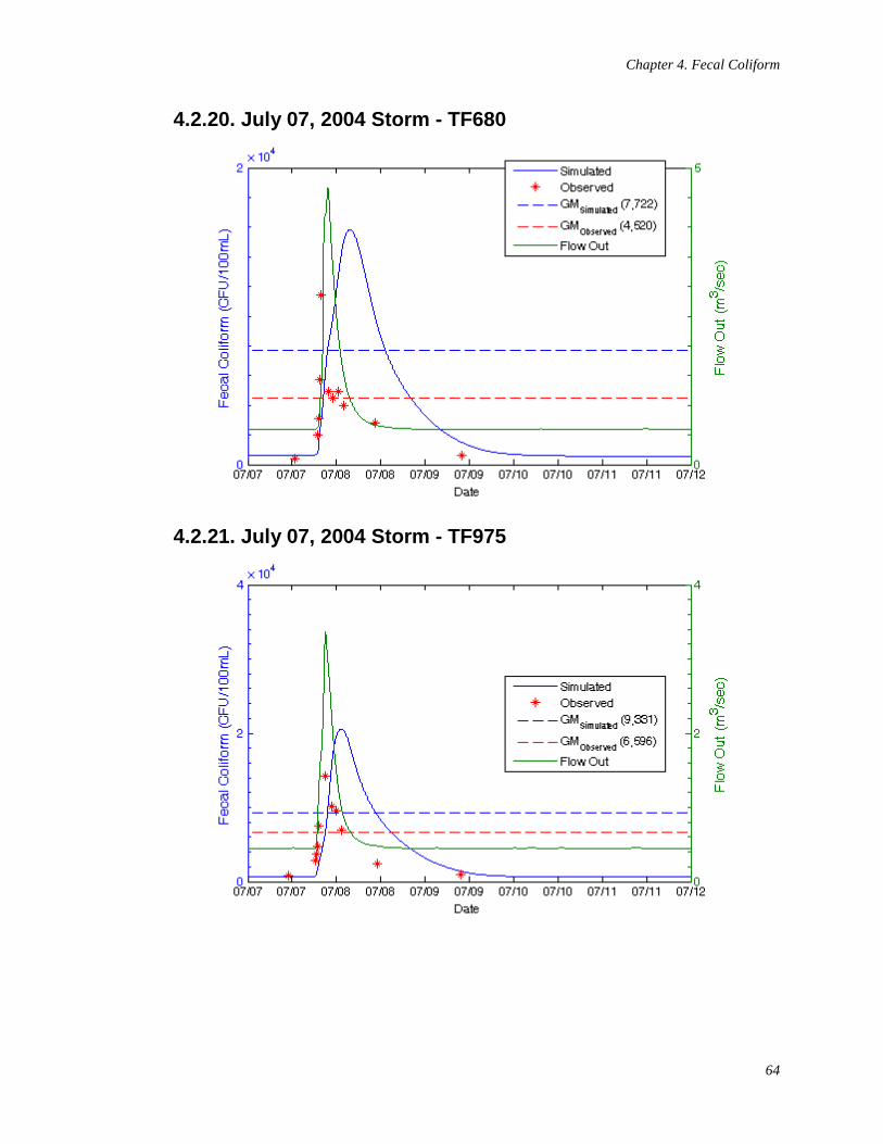
Chapter 4. Fecal Coliform
64
4.2.20. July 07, 2004 Storm - TF680
4.2.21. July 07, 2004 Storm - TF975
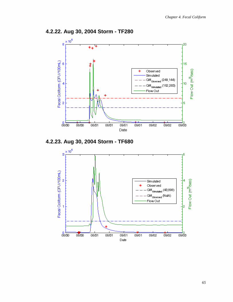
Chapter 4. Fecal Coliform
65
4.2.22. Aug 30, 2004 Storm - TF280
4.2.23. Aug 30, 2004 Storm - TF680
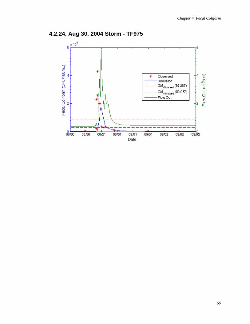
Chapter 4. Fecal Coliform
66
4.2.24. Aug 30, 2004 Storm - TF975
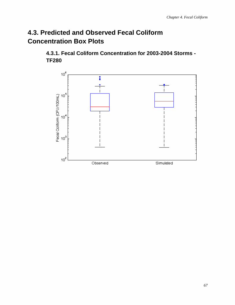
Chapter 4. Fecal Coliform
67
4.3. Predicted and Observed Fecal Coliform Concentration Box Plots
4.3.1. Fecal Coliform Concentration for 2003-2004 Storms - TF280
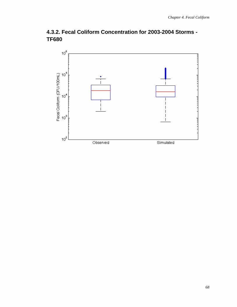
Chapter 4. Fecal Coliform
68
4.3.2. Fecal Coliform Concentration for 2003-2004 Storms - TF680
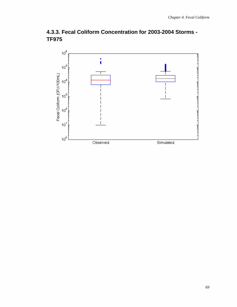
Chapter 4. Fecal Coliform
69
4.3.3. Fecal Coliform Concentration for 2003-2004 Storms - TF975
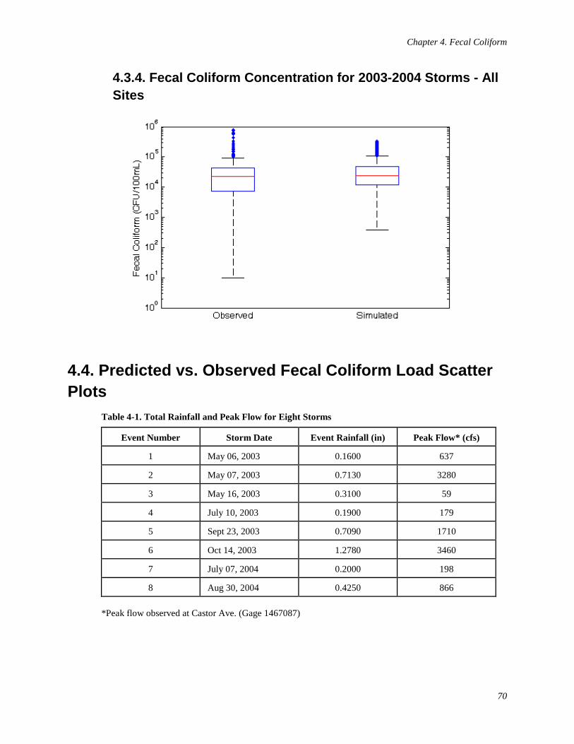
Chapter 4. Fecal Coliform
70
4.3.4. Fecal Coliform Concentration for 2003-2004 Storms - All Sites
4.4. Predicted vs. Observed Fecal Coliform Load Scatter Plots
Table 4-1. Total Rainfall and Peak Flow for Eight Storms
Event Number Storm Date Event Rainfall (in) Peak Flow* (cfs)
1 May 06, 2003 0.1600 637
2 May 07, 2003 0.7130 3280
3 May 16, 2003 0.3100 59
4 July 10, 2003 0.1900 179
5 Sept 23, 2003 0.7090 1710
6 Oct 14, 2003 1.2780 3460
7 July 07, 2004 0.2000 198
8 Aug 30, 2004 0.4250 866
*Peak flow observed at Castor Ave. (Gage 1467087)
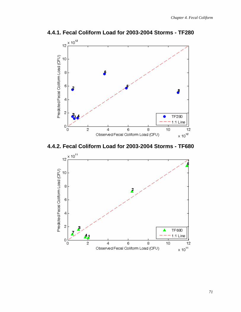
Chapter 4. Fecal Coliform
71
4.4.1. Fecal Coliform Load for 2003-2004 Storms - TF280
4.4.2. Fecal Coliform Load for 2003-2004 Storms - TF680
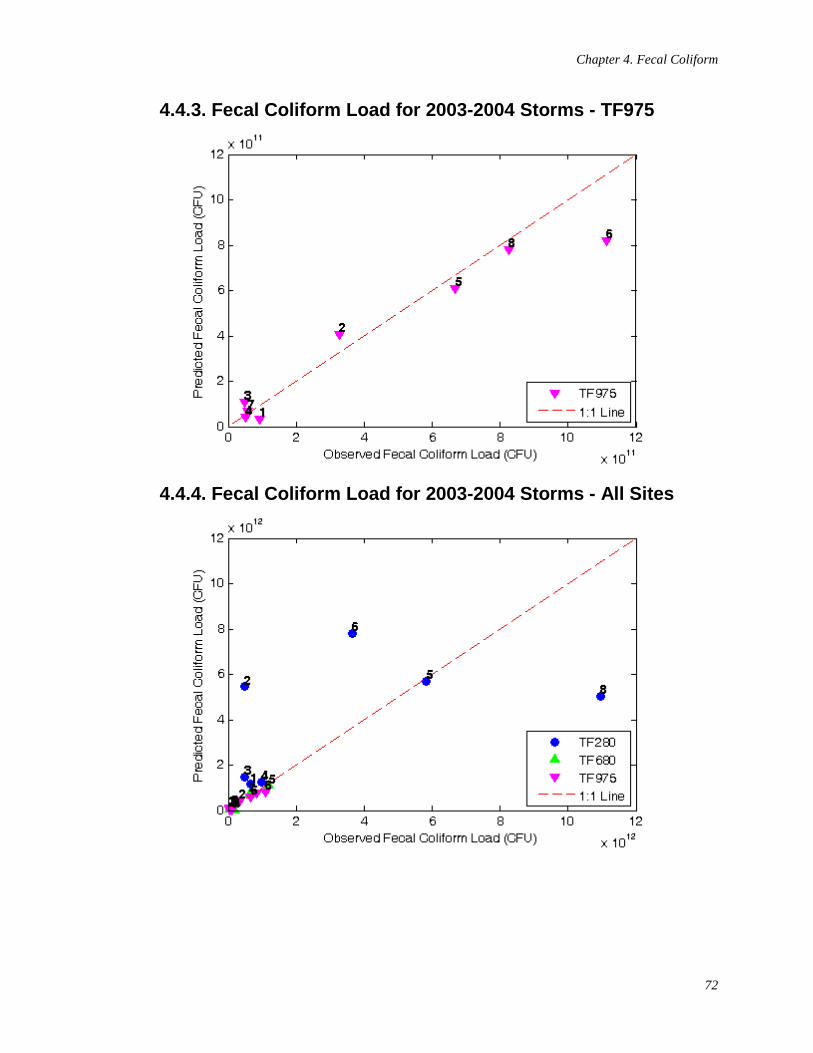
Chapter 4. Fecal Coliform
72
4.4.3. Fecal Coliform Load for 2003-2004 Storms - TF975
4.4.4. Fecal Coliform Load for 2003-2004 Storms - All Sites
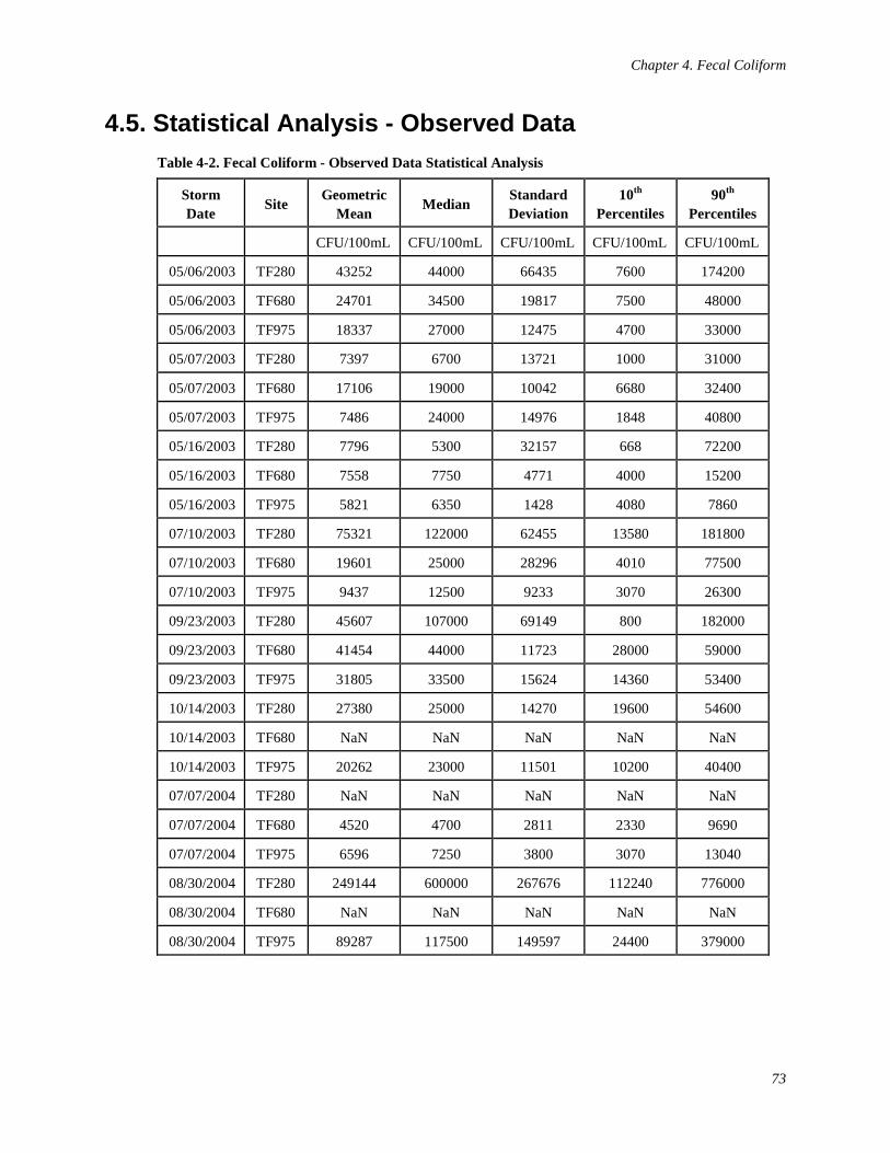
Chapter 4. Fecal Coliform
73
4.5. Statistical Analysis - Observed Data Table 4-2. Fecal Coliform - Observed Data Statistical Analysis
Storm Date Site Geometric
Mean Median Standard Deviation
10th Percentiles
90th Percentiles
CFU/100mL CFU/100mL CFU/100mL CFU/100mL CFU/100mL
05/06/2003 TF280 43252 44000 66435 7600 174200
05/06/2003 TF680 24701 34500 19817 7500 48000
05/06/2003 TF975 18337 27000 12475 4700 33000
05/07/2003 TF280 7397 6700 13721 1000 31000
05/07/2003 TF680 17106 19000 10042 6680 32400
05/07/2003 TF975 7486 24000 14976 1848 40800
05/16/2003 TF280 7796 5300 32157 668 72200
05/16/2003 TF680 7558 7750 4771 4000 15200
05/16/2003 TF975 5821 6350 1428 4080 7860
07/10/2003 TF280 75321 122000 62455 13580 181800
07/10/2003 TF680 19601 25000 28296 4010 77500
07/10/2003 TF975 9437 12500 9233 3070 26300
09/23/2003 TF280 45607 107000 69149 800 182000
09/23/2003 TF680 41454 44000 11723 28000 59000
09/23/2003 TF975 31805 33500 15624 14360 53400
10/14/2003 TF280 27380 25000 14270 19600 54600
10/14/2003 TF680 NaN NaN NaN NaN NaN
10/14/2003 TF975 20262 23000 11501 10200 40400
07/07/2004 TF280 NaN NaN NaN NaN NaN
07/07/2004 TF680 4520 4700 2811 2330 9690
07/07/2004 TF975 6596 7250 3800 3070 13040
08/30/2004 TF280 249144 600000 267676 112240 776000
08/30/2004 TF680 NaN NaN NaN NaN NaN
08/30/2004 TF975 89287 117500 149597 24400 379000
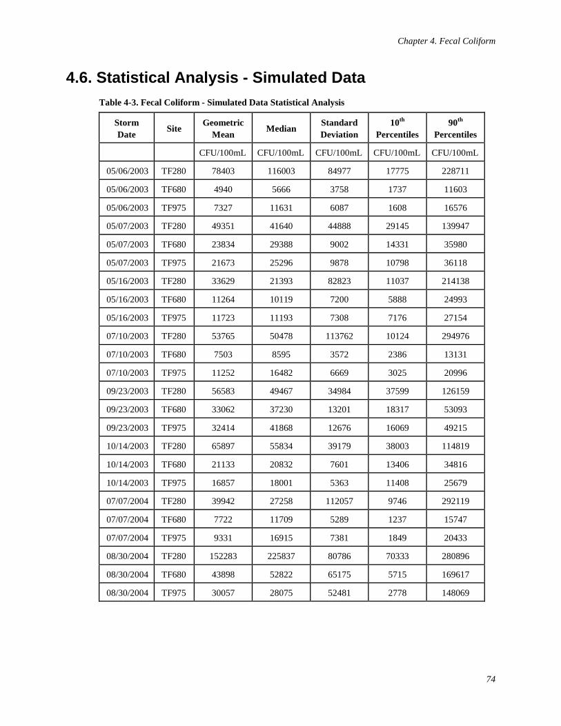
Chapter 4. Fecal Coliform
74
4.6. Statistical Analysis - Simulated Data Table 4-3. Fecal Coliform - Simulated Data Statistical Analysis
Storm Date Site Geometric
Mean Median Standard Deviation
10th Percentiles
90th Percentiles
CFU/100mL CFU/100mL CFU/100mL CFU/100mL CFU/100mL
05/06/2003 TF280 78403 116003 84977 17775 228711
05/06/2003 TF680 4940 5666 3758 1737 11603
05/06/2003 TF975 7327 11631 6087 1608 16576
05/07/2003 TF280 49351 41640 44888 29145 139947
05/07/2003 TF680 23834 29388 9002 14331 35980
05/07/2003 TF975 21673 25296 9878 10798 36118
05/16/2003 TF280 33629 21393 82823 11037 214138
05/16/2003 TF680 11264 10119 7200 5888 24993
05/16/2003 TF975 11723 11193 7308 7176 27154
07/10/2003 TF280 53765 50478 113762 10124 294976
07/10/2003 TF680 7503 8595 3572 2386 13131
07/10/2003 TF975 11252 16482 6669 3025 20996
09/23/2003 TF280 56583 49467 34984 37599 126159
09/23/2003 TF680 33062 37230 13201 18317 53093
09/23/2003 TF975 32414 41868 12676 16069 49215
10/14/2003 TF280 65897 55834 39179 38003 114819
10/14/2003 TF680 21133 20832 7601 13406 34816
10/14/2003 TF975 16857 18001 5363 11408 25679
07/07/2004 TF280 39942 27258 112057 9746 292119
07/07/2004 TF680 7722 11709 5289 1237 15747
07/07/2004 TF975 9331 16915 7381 1849 20433
08/30/2004 TF280 152283 225837 80786 70333 280896
08/30/2004 TF680 43898 52822 65175 5715 169617
08/30/2004 TF975 30057 28075 52481 2778 148069
Appendix D
Cobbs Creek Bacteria Model Validation
Simulations

Appendix D: Cobbs Creek Bacteria Model Validation Simulations:
This report compares observed bacteria data and WASP predicted outputs for the following four storms: Jul 26, 2000, Jul 23, 2003, Jul 24, 2003 and Sept 13, 2003.
iii
Table of Contents 1. General Information ............................................................................................................................. 1
1.1. Segmentation Map ..................................................................................................................... 2 2. E. coli ..................................................................................................................................................... 3
2.1. E. coli Time Series ..................................................................................................................... 3 2.1.1. July 26, 2000 Storm - DCC110 ..................................................................................... 3 2.1.2. July 23, 2003 Storm - DCC208 ..................................................................................... 4 2.1.3. July 23, 2003 Storm - DCC455 ..................................................................................... 4 2.1.4. July 24, 2003 Storm - DCC208 ..................................................................................... 5 2.1.5. July 24, 2003 Storm - DCC455 ..................................................................................... 5 2.1.6. Sept 13, 2003 Storm - DCC208 ..................................................................................... 6 2.1.7. Sept 13, 2003 Storm - DCC455 ..................................................................................... 6
2.2. E. coli and Flow Out Time Series .............................................................................................. 7 2.2.1. July 26, 2000 Storm - DCC110 ..................................................................................... 7 2.2.2. July 23, 2003 Storm - DCC208 ..................................................................................... 7 2.2.3. July 23, 2003 Storm - DCC455 ..................................................................................... 8 2.2.4. July 24, 2003 Storm - DCC208 ..................................................................................... 8 2.2.5. July 24, 2003 Storm - DCC455 ..................................................................................... 9 2.2.6. Sept 13, 2003 Storm - DCC208 ..................................................................................... 9 2.2.7. Sept 13, 2003 Storm - DCC455 ................................................................................... 10
2.3. Predicted and Observed E. coli Concentration Box Plots ........................................................ 11 2.3.1. E. coli Concentration for 2003-2004 Storms - DCC208 .............................................. 11 2.3.2. E. coli Concentration for 2003-2004 Storms - DCC455 .............................................. 11 2.3.3. E. coli Concentration for 2003-2004 Storms - All Sites .............................................. 12
2.4. Predicted vs. Observed E. coli Load Scatter Plots ................................................................... 12 2.4.1. E. coli Load for 2003-2004 Storms - DCC208 ............................................................ 13 2.4.2. E. coli Load for 2003-2004 Storms - DCC455 ............................................................ 13 2.4.3. E. coli Load for 2003-2004 Storms - All Sites ............................................................ 14
2.5. Statistical Analysis ................................................................................................................... 14 3. Fecal Coliform .................................................................................................................................... 16
3.1. Fecal Coliform Time Series ..................................................................................................... 16 3.1.1. July 26, 2000 Storm - DCC110 ................................................................................... 16 3.1.2. July 23, 2003 Storm - DCC208 ................................................................................... 17 3.1.3. July 23, 2003 Storm - DCC455 ................................................................................... 17 3.1.4. July 24, 2003 Storm - DCC208 ................................................................................... 18 3.1.5. July 24, 2003 Storm - DCC455 ................................................................................... 18 3.1.6. Sept 13, 2003 Storm - DCC208 ................................................................................... 19 3.1.7. Sept 13, 2003 Storm - DCC455 ................................................................................... 19
3.2. Fecal Coliform and Flow Out Time Series .............................................................................. 20 3.2.1. July 26, 2000 Storm - DCC110 ................................................................................... 20 3.2.2. July 23, 2003 Storm - DCC208 ................................................................................... 20 3.2.3. July 23, 2003 Storm - DCC455 ................................................................................... 21 3.2.4. July 24, 2003 Storm - DCC208 ................................................................................... 21 3.2.5. July 24, 2003 Storm - DCC455 ................................................................................... 22
iv
3.2.6. Sept 13, 2003 Storm - DCC208 ................................................................................... 22 3.2.7. Sept 13, 2003 Storm - DCC455 ................................................................................... 23
3.3. Predicted and Observed Fecal Coliform Concentration Box Plots .......................................... 24 3.3.1. Fecal Coliform Concentration for 2003-2004 Storms - DCC208 ................................ 24 3.3.2. Fecal Coliform Concentration for 2003-2004 Storms - DCC455 ................................ 25 3.3.3. Fecal Coliform Concentration for 2003-2004 Storms - All Sites ................................ 25
3.4. Predicted vs. Observed Fecal Coliform Load Scatter Plots...................................................... 26 3.4.1. Fecal Coliform Load for 2003-2004 Storms - DCC208 .............................................. 26 3.4.2. Fecal Coliform Load for 2003-2004 Storms - DCC455 .............................................. 27 3.4.3. Fecal Coliform Load for 2003-2004 Storms - All Sites............................................... 27
3.5. Statistical Analysis ................................................................................................................... 28
v
List of Tables 1-1. Cobbs Monitoring Locations .............................................................................................................. 1 2-1. Total Rainfall and Peak Flow for Four Storms ................................................................................. 12 2-2. E. coli - Observed Data Statistical Analysis ..................................................................................... 14 2-3. E. coli - Predicted Data Statistical Analysis ..................................................................................... 15 3-1. Total Rainfall and Peak Flow for Four Storms ................................................................................. 26 3-2. Fecal Coliform - Observed Data Statistical Analysis ....................................................................... 28 3-3. Fecal Coliform - Predicted Data Statistical Analysis ....................................................................... 28

1
Chapter 1. General Information Table 1-1. Cobbs Monitoring Locations
Site ID Loc ID WASP Segment
DCC110 COBB175 Segment 19
DCC208 COBB350 Segment 16
DCC455 COBB550 Segment 09
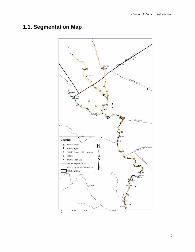
Chapter 1. General Information
2
1.1. Segmentation Map
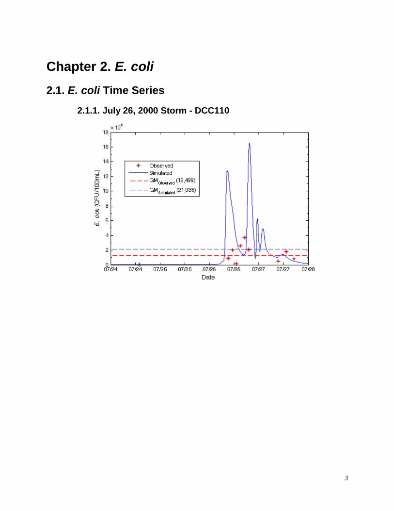
3
Chapter 2. E. coli
2.1. E. coli Time Series
2.1.1. July 26, 2000 Storm - DCC110
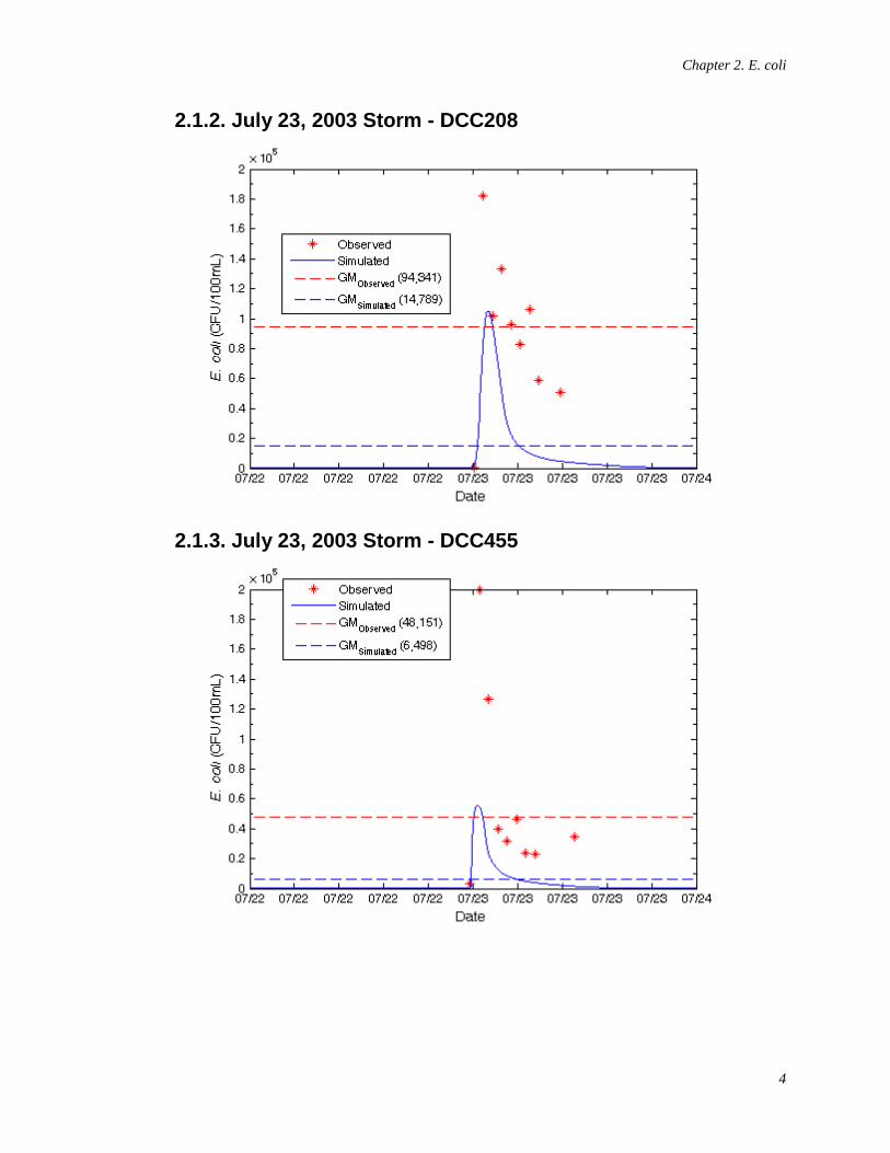
Chapter 2. E. coli
4
2.1.2. July 23, 2003 Storm - DCC208
2.1.3. July 23, 2003 Storm - DCC455
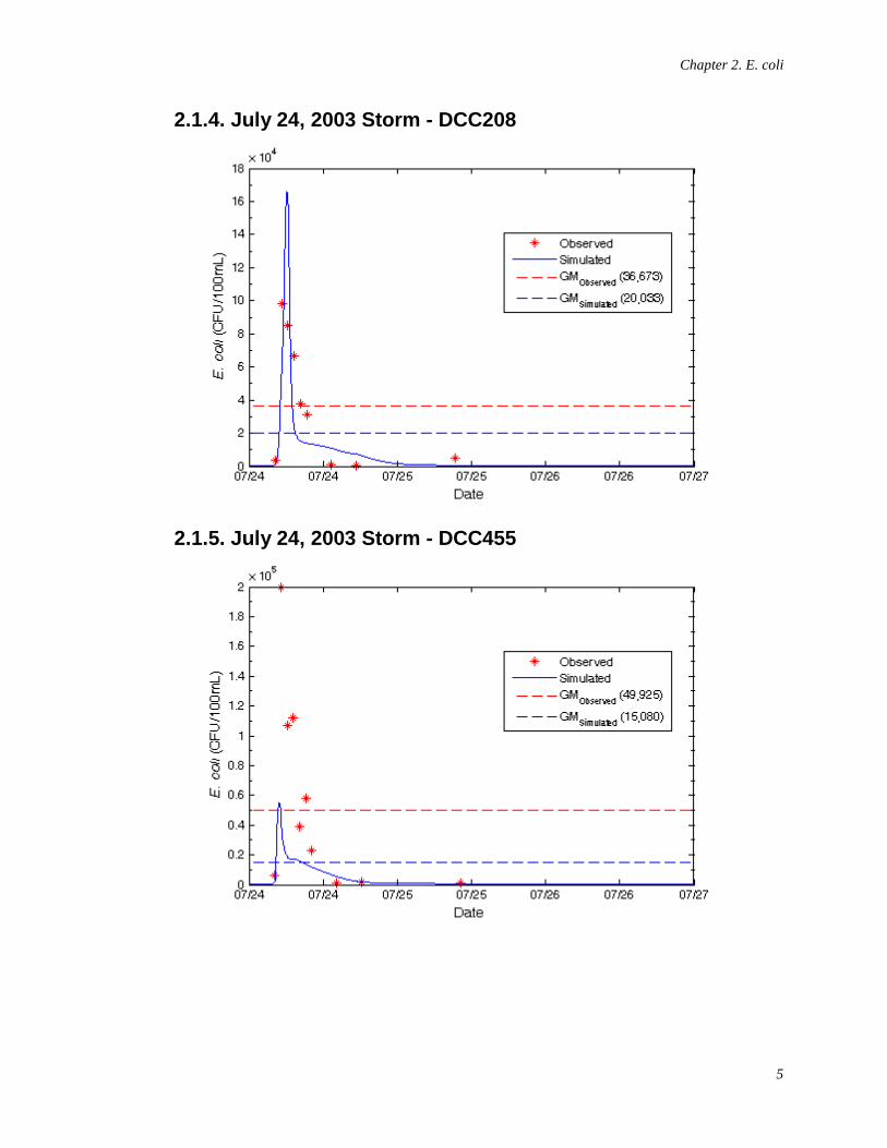
Chapter 2. E. coli
5
2.1.4. July 24, 2003 Storm - DCC208
2.1.5. July 24, 2003 Storm - DCC455
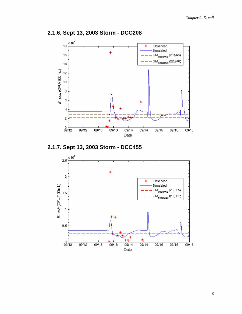
Chapter 2. E. coli
6
2.1.6. Sept 13, 2003 Storm - DCC208
2.1.7. Sept 13, 2003 Storm - DCC455
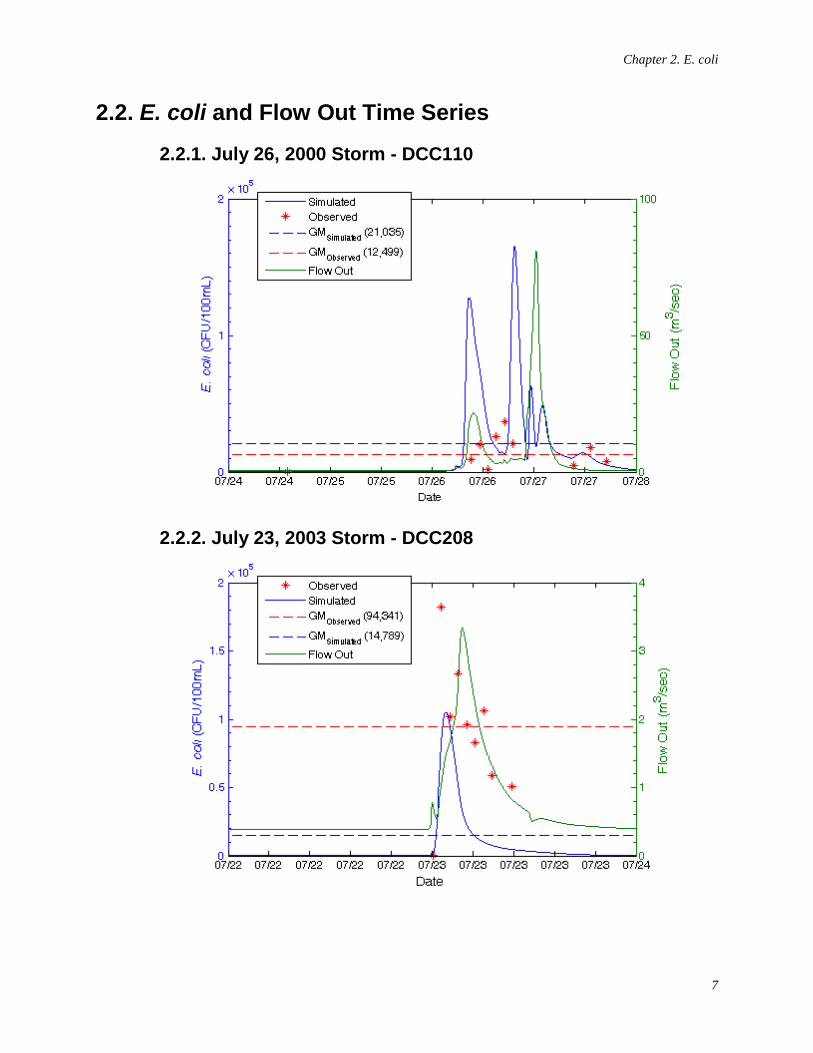
Chapter 2. E. coli
7
2.2. E. coli and Flow Out Time Series
2.2.1. July 26, 2000 Storm - DCC110
2.2.2. July 23, 2003 Storm - DCC208
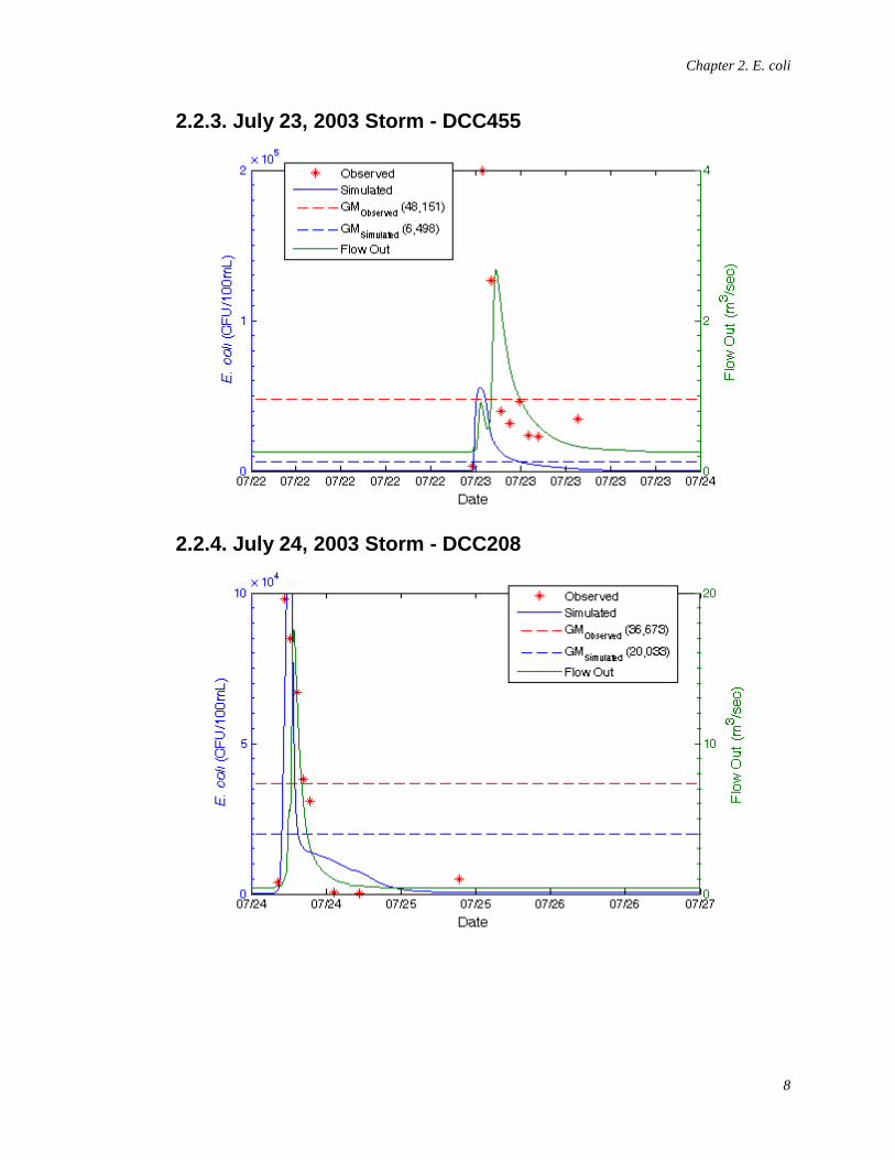
Chapter 2. E. coli
8
2.2.3. July 23, 2003 Storm - DCC455
2.2.4. July 24, 2003 Storm - DCC208
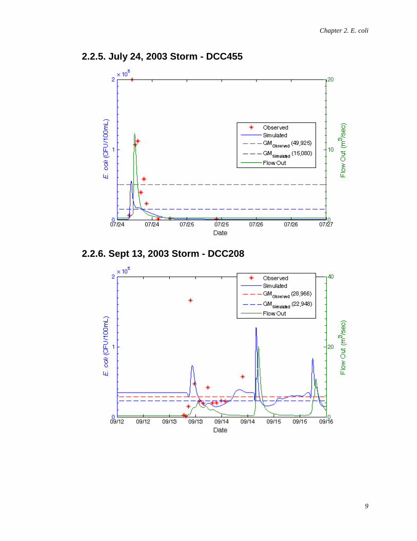
Chapter 2. E. coli
9
2.2.5. July 24, 2003 Storm - DCC455
2.2.6. Sept 13, 2003 Storm - DCC208
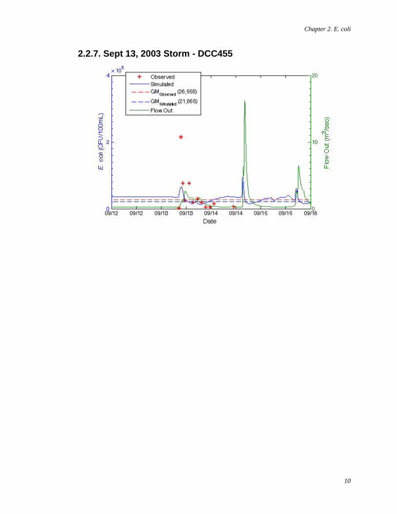
Chapter 2. E. coli
10
2.2.7. Sept 13, 2003 Storm - DCC455
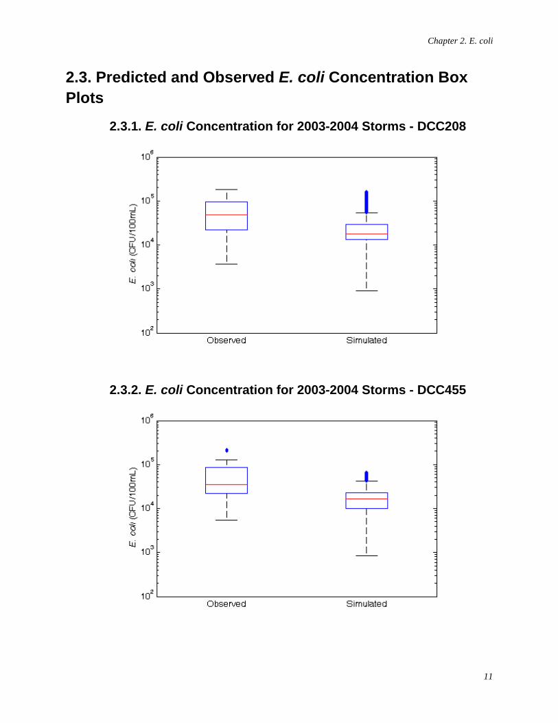
Chapter 2. E. coli
11
2.3. Predicted and Observed E. coli Concentration Box Plots
2.3.1. E. coli Concentration for 2003-2004 Storms - DCC208
2.3.2. E. coli Concentration for 2003-2004 Storms - DCC455
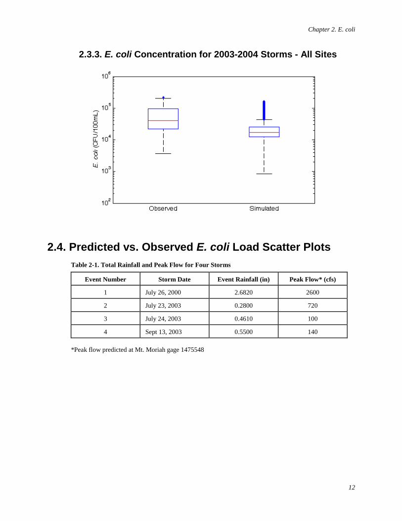
Chapter 2. E. coli
12
2.3.3. E. coli Concentration for 2003-2004 Storms - All Sites
2.4. Predicted vs. Observed E. coli Load Scatter Plots Table 2-1. Total Rainfall and Peak Flow for Four Storms
Event Number Storm Date Event Rainfall (in) Peak Flow* (cfs)
1 July 26, 2000 2.6820 2600
2 July 23, 2003 0.2800 720
3 July 24, 2003 0.4610 100
4 Sept 13, 2003 0.5500 140
*Peak flow predicted at Mt. Moriah gage 1475548
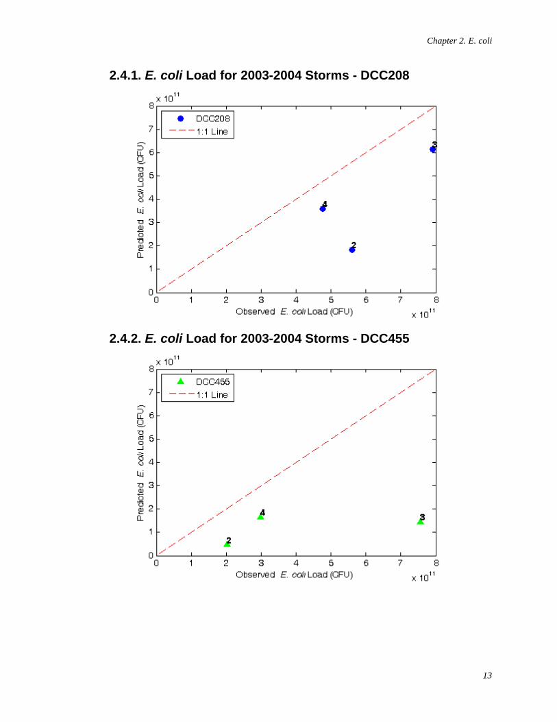
Chapter 2. E. coli
13
2.4.1. E. coli Load for 2003-2004 Storms - DCC208
2.4.2. E. coli Load for 2003-2004 Storms - DCC455
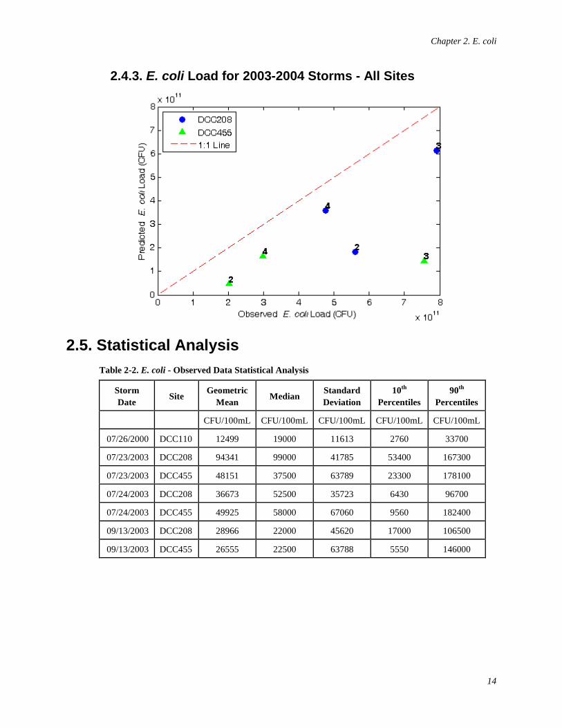
Chapter 2. E. coli
14
2.4.3. E. coli Load for 2003-2004 Storms - All Sites
2.5. Statistical Analysis Table 2-2. E. coli - Observed Data Statistical Analysis
Storm Date Site Geometric
Mean Median Standard Deviation
10th Percentiles
90th Percentiles
CFU/100mL CFU/100mL CFU/100mL CFU/100mL CFU/100mL
07/26/2000 DCC110 12499 19000 11613 2760 33700
07/23/2003 DCC208 94341 99000 41785 53400 167300
07/23/2003 DCC455 48151 37500 63789 23300 178100
07/24/2003 DCC208 36673 52500 35723 6430 96700
07/24/2003 DCC455 49925 58000 67060 9560 182400
09/13/2003 DCC208 28966 22000 45620 17000 106500
09/13/2003 DCC455 26555 22500 63788 5550 146000
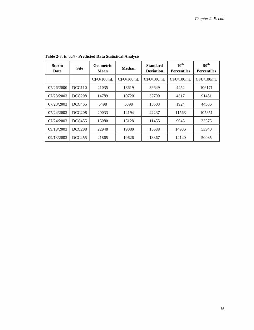
Chapter 2. E. coli
15
Table 2-3. E. coli - Predicted Data Statistical Analysis
Storm Date Site Geometric
Mean Median Standard Deviation
10th Percentiles
90th Percentiles
CFU/100mL CFU/100mL CFU/100mL CFU/100mL CFU/100mL
07/26/2000 DCC110 21035 18619 39649 4252 106171
07/23/2003 DCC208 14789 10720 32700 4317 91481
07/23/2003 DCC455 6498 5098 15503 1924 44506
07/24/2003 DCC208 20033 14194 42237 11568 105851
07/24/2003 DCC455 15080 15128 11455 9045 33575
09/13/2003 DCC208 22948 19080 15588 14906 53940
09/13/2003 DCC455 21865 19626 13367 14140 50085
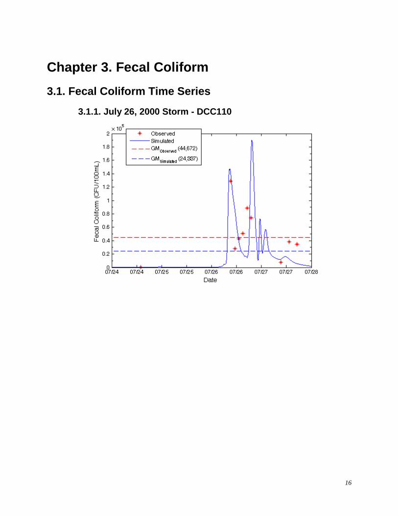
16
Chapter 3. Fecal Coliform
3.1. Fecal Coliform Time Series
3.1.1. July 26, 2000 Storm - DCC110
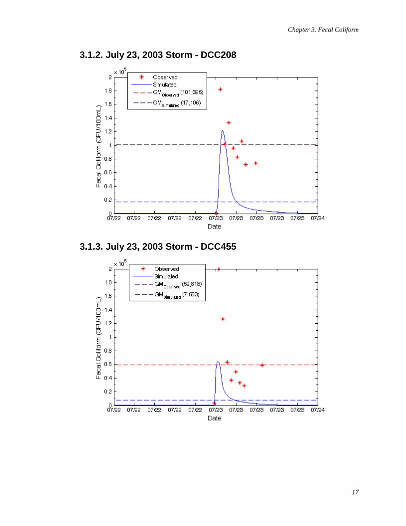
Chapter 3. Fecal Coliform
17
3.1.2. July 23, 2003 Storm - DCC208
3.1.3. July 23, 2003 Storm - DCC455
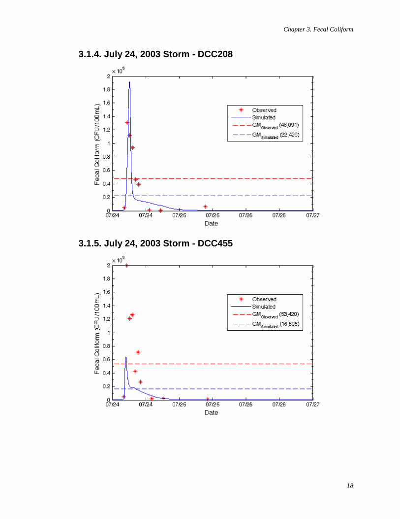
Chapter 3. Fecal Coliform
18
3.1.4. July 24, 2003 Storm - DCC208
3.1.5. July 24, 2003 Storm - DCC455
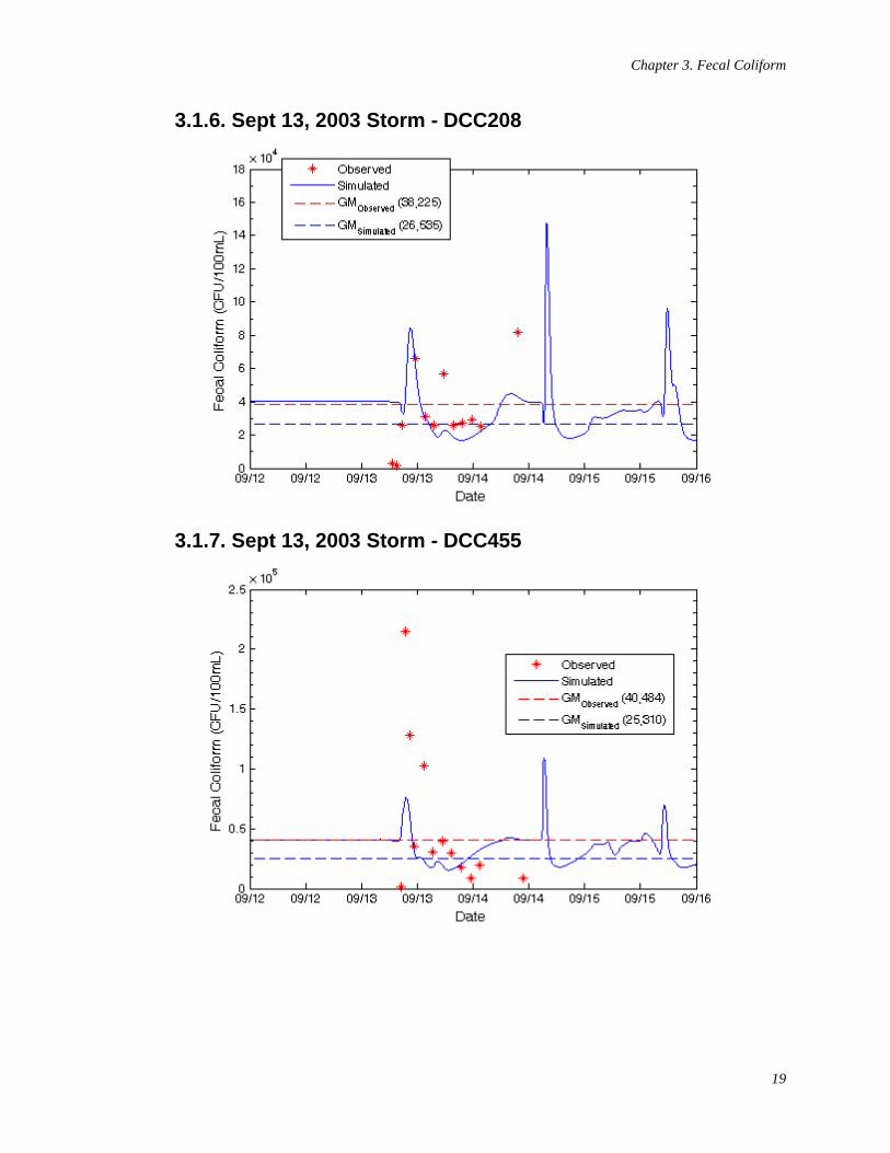
Chapter 3. Fecal Coliform
19
3.1.6. Sept 13, 2003 Storm - DCC208
3.1.7. Sept 13, 2003 Storm - DCC455
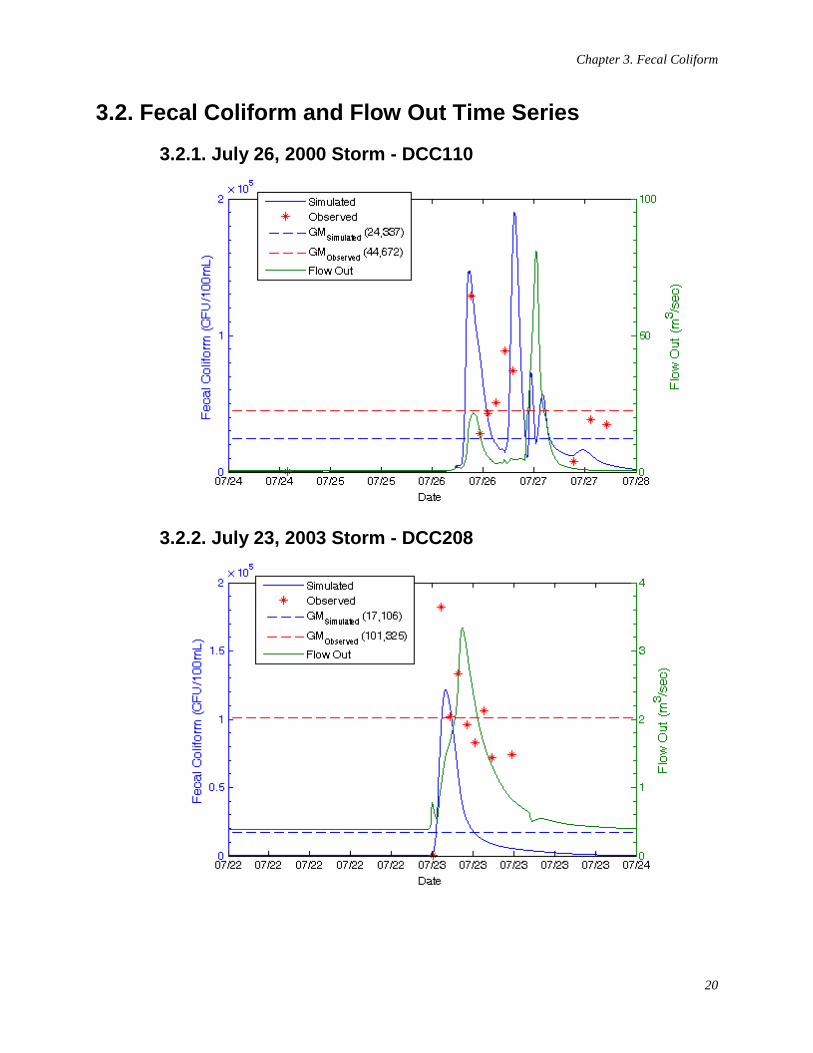
Chapter 3. Fecal Coliform
20
3.2. Fecal Coliform and Flow Out Time Series
3.2.1. July 26, 2000 Storm - DCC110
3.2.2. July 23, 2003 Storm - DCC208
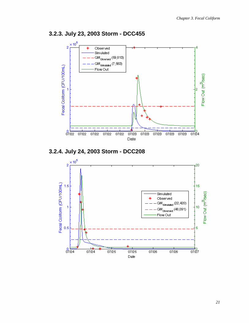
Chapter 3. Fecal Coliform
21
3.2.3. July 23, 2003 Storm - DCC455
3.2.4. July 24, 2003 Storm - DCC208
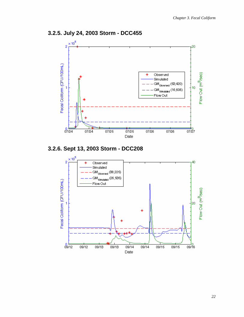
Chapter 3. Fecal Coliform
22
3.2.5. July 24, 2003 Storm - DCC455
3.2.6. Sept 13, 2003 Storm - DCC208
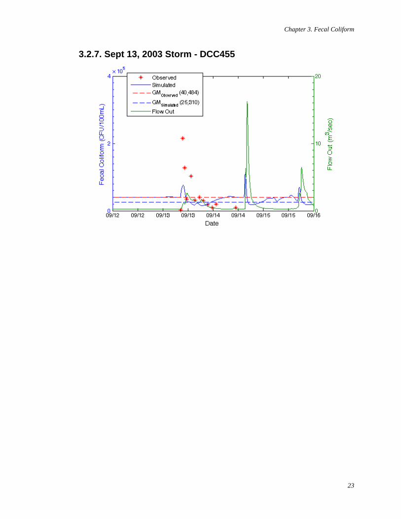
Chapter 3. Fecal Coliform
23
3.2.7. Sept 13, 2003 Storm - DCC455
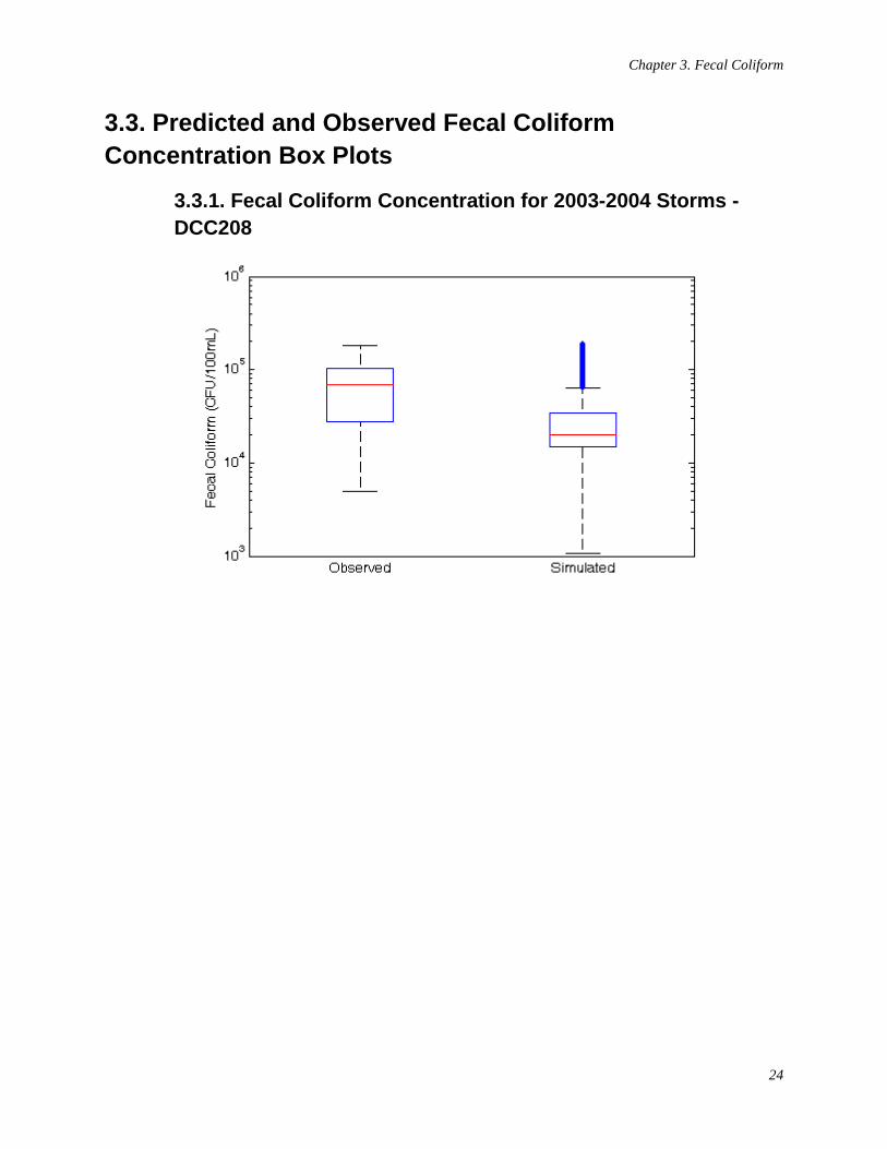
Chapter 3. Fecal Coliform
24
3.3. Predicted and Observed Fecal Coliform Concentration Box Plots
3.3.1. Fecal Coliform Concentration for 2003-2004 Storms - DCC208
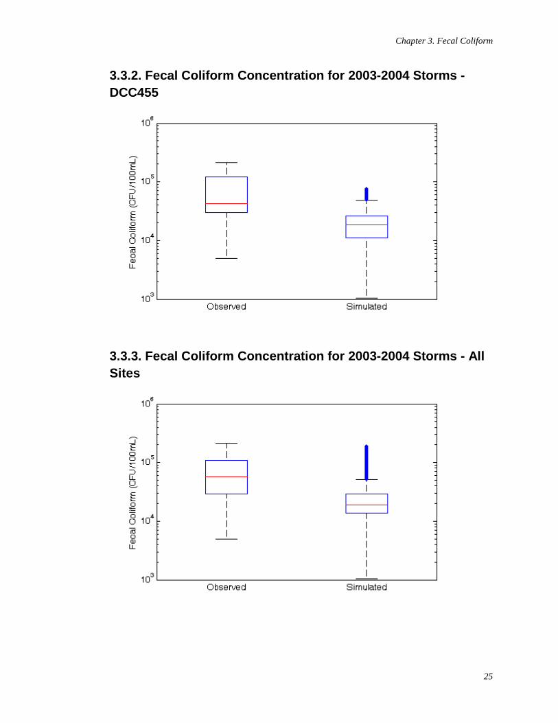
Chapter 3. Fecal Coliform
25
3.3.2. Fecal Coliform Concentration for 2003-2004 Storms - DCC455
3.3.3. Fecal Coliform Concentration for 2003-2004 Storms - All Sites
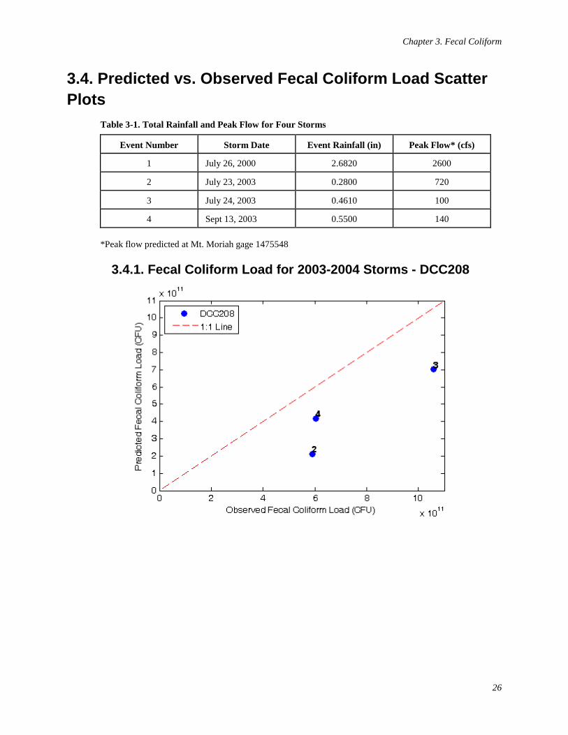
Chapter 3. Fecal Coliform
26
3.4. Predicted vs. Observed Fecal Coliform Load Scatter Plots
Table 3-1. Total Rainfall and Peak Flow for Four Storms
Event Number Storm Date Event Rainfall (in) Peak Flow* (cfs)
1 July 26, 2000 2.6820 2600
2 July 23, 2003 0.2800 720
3 July 24, 2003 0.4610 100
4 Sept 13, 2003 0.5500 140
*Peak flow predicted at Mt. Moriah gage 1475548
3.4.1. Fecal Coliform Load for 2003-2004 Storms - DCC208
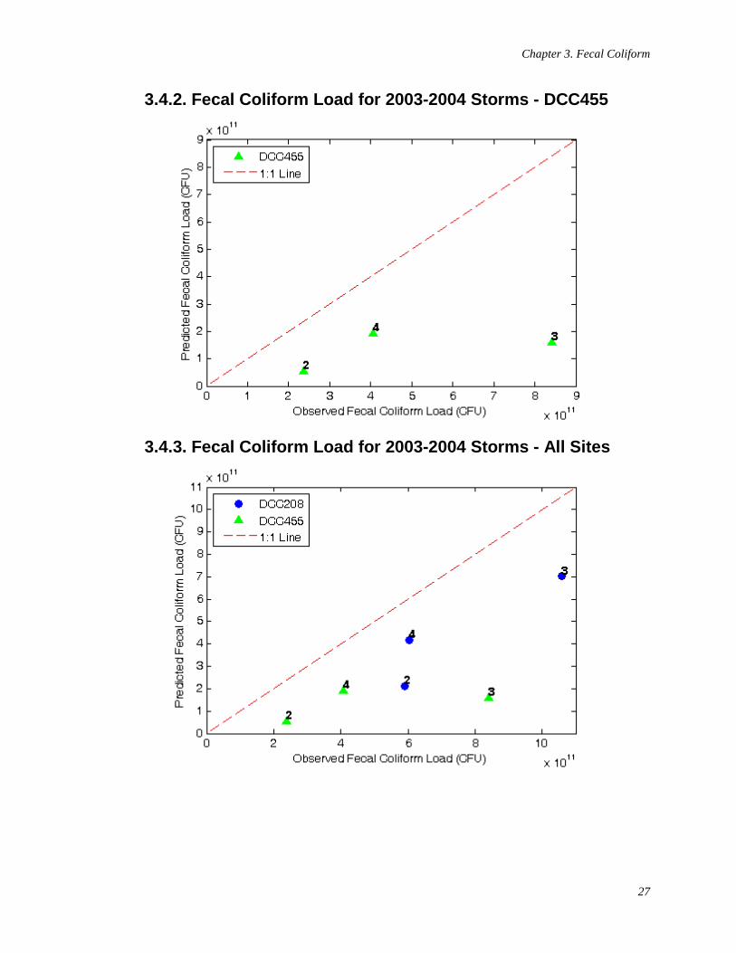
Chapter 3. Fecal Coliform
27
3.4.2. Fecal Coliform Load for 2003-2004 Storms - DCC455
3.4.3. Fecal Coliform Load for 2003-2004 Storms - All Sites

Chapter 3. Fecal Coliform
28
3.5. Statistical Analysis Table 3-2. Fecal Coliform - Observed Data Statistical Analysis
Storm Date Site Geometric
Mean Median Standard Deviation
10th Percentiles
90th Percentiles
CFU/100mL CFU/100mL CFU/100mL CFU/100mL CFU/100mL
07/26/2000 DCC110 44672 47000 38415 14000 117000
07/23/2003 DCC208 101325 99000 36508 72600 167300
07/23/2003 DCC455 59813 54000 59435 30200 178100
07/24/2003 DCC208 48091 70000 48610 8400 129100
07/24/2003 DCC455 53420 71000 68343 9320 185400
09/13/2003 DCC208 38225 28000 43971 25500 116000
09/13/2003 DCC455 40484 33000 65959 13450 171500
Table 3-3. Fecal Coliform - Predicted Data Statistical Analysis
Storm Date Site Geometric
Mean Median Standard Deviation
10th Percentiles
90th Percentiles
CFU/100mL CFU/100mL CFU/100mL CFU/100mL CFU/100mL
07/26/2000 DCC110 24337 21499 45748 4928 122522
07/23/2003 DCC208 17106 12390 37728 5011 105577
07/23/2003 DCC455 7563 5915 17881 2270 51375
07/24/2003 DCC208 22420 15617 48937 12689 122015
07/24/2003 DCC455 16606 16392 13406 9869 38541
09/13/2003 DCC208 26535 22070 17977 17256 62270
09/13/2003 DCC455 25310 22725 15412 16394 57839