Appendix A The Capital Asset Pricing Model (CAPM)978-1-4471-6305...Appendix A The Capital Asset...

Appendix AThe Capital Asset Pricing Model (CAPM)

The CAPM has historical significance, but it is only very restrictedly suitable formodern risk management because of its considerable simplifications.

We assume that the market consists in n + 1 financial instruments i ∈ {0, . . . , n}.Denote by Pi the “normed” investment in the financial instrument i that has (attime 0) the value 1. We represent Pi by the (1 + i)-th unit vector in R

n+1. Thereturn (at time 1) from this investment is a random variable that we denote by Ri .we make the following economic assumptions:

(i) For the financial instrument 0 the return R0 is constant. P0 is thus a risk-freeinvestment. On competitive grounds there can be at most one risk-free financialinstrument.

(ii) For all i > 0 we have var(Ri) > 0. The investments P1, . . . ,Pn are called risky.(iii) The returns on financial instruments are positively correlated, but not perfectly,

corr(Ri,Rj ) ∈ [0,1[ for all i, j .(iv) There are neither transaction costs nor personal income tax.(v) Any investment can be arbitrarily divided.

(vi) There is perfect competition: No single investor can influence the share pricesby buying or selling.

(vii) Each investor bases his decisions only upon the expectation values and vari-ances of the returns of all possible portfolios.

Definition A.1 A portfolio P(x) = ∑ni=0 xiPi consists in xi ≥ 0 shares in the in-

vestment Pi for each i ∈ {0, . . . , n}. We denote the return on P(x) by R(x).A pure portfolio P(x) is a portfolio of investments with x0 = 0. We denote the

set of all pure portfolios by Ppure.A normed portfolio is a portfolio P(x) with

∑ni=0 xi = 1. We denote the set of

all normed portfolios by Pnorm.

Remark A.1 Obviously the value of a normed portfolio is 1.

M. Kriele, J. Wolf, Value-Oriented Risk Management of Insurance Companies,EAA Series, DOI 10.1007/978-1-4471-6305-3, © Springer-Verlag London 2014

335

http://dx.doi.org/10.1007/978-1-4471-6305-3

336 A The Capital Asset Pricing Model (CAPM)

For P(x),P (y) ∈ Pnorm let

P(x) ≺ P(y) ⇔

⎧⎪⎨

⎪⎩

E(R(x)) < E(R(y)), σ (R(x)) ≥ σ(R(y))

or

E(R(x)) ≤ E(R(y)), σ (R(x)) > σ(R(y)).

If P(x) ≺ P(y), then (under the fundamental assumptions of CAPM) the normedportfolio P(y) is to be preferred over the normed portfolio P(x). The optimalboundary ∂Pnorm of Pnorm consists in the portfolios

∂Pnorm = {P(x) ∈ Pnorm : there is no P(y) ∈ Pnorm with P(x) ≺ P(y)

}

Since [0,1]n+1 ∩ {x : ∑ni=1 xi = 1} is compact, ∂Pnorm is well-defined.

The optimal boundary ∂Pnormpure of Pnorm

pure = Pnorm ∩ Ppure is analogously de-fined.

Definition A.2 Let P(x) be a normed portfolio. Then

p(x) = (σ(R(x)

),E

(R(x)

)) ∈R2

is a point in the risk-return diagram of the capital market.The capital market line is the set

{p(x) ∈ R

2 : P(x) ∈ ∂Pnorm}

in the risk-return diagram.The efficient frontier is the set

{p(x) ∈ R

2 : P(x) ∈ ∂Pnormpure

}.

in the risk-return diagram.We say that P(x) lies on the capital market line or the efficient frontier if

(σ(R(x)

),E

(R(x)

)

is a point on the capital market line or the efficient frontier.

The capital market line describes the investment portfolios that are optimal in themarket.

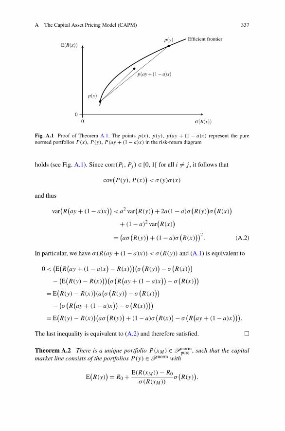
Theorem A.1 The efficient frontier is concave.

Proof Let P(x) and P(y) be pure normed portfolios on the efficient frontier. Wecan assume, without loss of generality, that σ(R(y)) > σ(R(x)) and E(R(y)) >

E(R(x)). It suffices to show that for a ∈]0,1[E(R(ay + (1 − a)x) − R(x))

σ (R(ay + (1 − a)x)) − σ(R(x))>

E(R(y) − R(x))

σ (R(y)) − σ(R(x))(A.1)

A The Capital Asset Pricing Model (CAPM) 337

Fig. A.1 Proof of Theorem A.1. The points p(x), p(y), p(ay + (1 − a)x) represent the purenormed portfolios P (x), P (y), P (ay + (1 − a)x) in the risk-return diagram

holds (see Fig. A.1). Since corr(Pi,Pj ) ∈ [0,1[ for all i �= j , it follows that

cov(P(y),P (x)

)< σ(y)σ (x)

and thus

var(R

(ay + (1 − a)x

))< a2 var

(R(y)

) + 2a(1 − a)σ(R(y)

)σ(R(x)

)

+ (1 − a)2 var(R(x)

)

= (aσ

(R(y)

) + (1 − a)σ(R(x)

))2. (A.2)

In particular, we have σ(R(ay + (1 − a)x)) < σ(R(y)) and (A.1) is equivalent to

0 <(E(R

(ay + (1 − a)x

) − R(x)))(

σ(R(y)

) − σ(R(x)

))

− (E(R(y) − R(x)

))(σ(R

(ay + (1 − a)x

)) − σ(R(x)

))

= E(R(y) − R(x)

)(a

(σ(R(y)

) − σ(R(x)

))

− (σ(R

(ay + (1 − a)x

)) − σ(R(x)

)))

= E(R(y) − R(x)

)(aσ

(R(y)

) + (1 − a)σ(R(x)

) − σ(R

(ay + (1 − a)x

))).

The last inequality is equivalent to (A.2) and therefore satisfied. �

Theorem A.2 There is a unique portfolio P(xM) ∈ Pnormpure , such that the capital

market line consists of the portfolios P(y) ∈ Pnorm with

E(R(y)

) = R0 + E(R(xM)) − R0

σ(R(xM))σ(R(y)

).


Proof Each normed portfolio P(y) has the form P(y) = aP0 + (1−a)P (x), whereP(x) is a pure normed portfolio and a ∈ [0,1] holds. We have

E(R(y)

) = aR0 + (1 − a)E(R(x)

) = R0 + (1 − a)(E(R(x)

) − R0), (A.3)

where we used E(R0) = R0. Since aR0 is a constant random variable, we obtain

var(R(y)

) = var(aR0 + (1 − a)R(x)

) = (1 − a)2 var(R(x)

)

resp. σ(R(y)) = (1 − a)σ (R(x)). By solving this equation for 1 − a and puttingthat in (A.3), we see that in the risk-return diagram the points p(y) of the portfoliosP(y), that are for fixed x a combination of P(x) and P0, lie on a line. This line isgiven by

E(R(y) = R0 + E(R(x)) − R0

σ(R(x))σ(R(y)

).

In particular, the point (0,R0) lies on the line and does not depend on P(x). There-fore each line which arises in this way from a pure normed portfolio P(x) goesthrough (0,R0). Let j > 0 be the financial instrument for which the return on thenormed investment Pj has the smallest standard deviation σ(Rj ) > 0, and let i bethe financial instrument for which the return on the normed investment Pi has thelargest expected value E(Ri). Then we have for the slope θ(x) of the line generatedby P(x)

θ(x) = E(R(x)) − R0

σ(R(x)) − σ(R0)= E(R(x)) − R0

σ(R(x))≤ Ri − R0

σ(Rj )< ∞.

Therefore there exists

θmax = sup{θ(x) : P(x) ∈ Pnorm

pure

}< ∞.

Since [0,1]n+1 ∩ {x : x0 = 0,∑n

i=0 xi = 1} compact and x → θ(x) is continuous,there exists a sequence {xk}k∈N converging to a vector xM , so that

(i) P(xk) and P(xM) are pure normed portfolios,(ii) θ(xM) = θmax,

(iii) P(xM) lies on the capital market line.

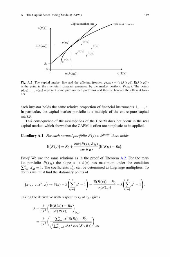
See Fig. A.2. Because P(xM) lies on the capital market line, the capital marketline is tangent to the efficient frontier. P(xM) is unique, because the tangents to aconcave curve each touch the curve at a single point. �

Definition A.3 P(xM) is the market portfolio. We write RM = R(xM).

Since in CAPM each investor makes decisions exclusively from the expectedvalues and variances of the possible portfolios, it is optimal for each investor toinvest in a mixture of the market portfolio and risk-free investments. It follows that


Fig. A.2 The capital market line and the efficient frontier. p(xM) = (σ (R(xM)),E(R(xM)))

is the point in the risk-return diagram generated by the market portfolio P (xM). The pointsp(y1), . . . , p(y5) represent some pure normed portfolios and thus lie beneath the efficient fron-tier

each investor holds the same relative proportion of financial instruments 1, . . . , n.In particular, the capital market portfolio is a multiple of the entire pure capitalmarket.

This consequence of the assumptions of the CAPM does not occur in the realcapital market, which shows that the CAPM is often too simplistic to be applied.

Corollary A.1 For each normed portfolio P(y) ∈ Pnorm there holds

E(R(y)

) = R0 + cov(R(y),RM)

var(RM)

(E(RM) − R0

).

Proof We use the same relations as in the proof of Theorem A.2. For the mar-ket portfolio P(xM) the slope x → θ(x) has maximum under the condition∑n

i=1 xiM = 1. The coefficients xi

M can be determined as Lagrange multipliers. Todo this we must find the stationary points of

(x1, . . . , xn, λ

) → θ(x) − λ

(n∑

i=1

xi − 1

)

= E(R(x)) − R0

σ(R(x))− λ

(n∑

i=1

xi − 1

)

.

Taking the derivative with respect to xk at xM gives

λ = ∂

∂xk

(E(R(x)) − R0

σ(R(x))

)

|xM

= ∂

∂xk

( ∑ni=1 xi E(Ri) − R0

√∑ni,j=1 xixj cov(Ri,Rj )

)

|xM


= E(Rk)σ (RM) − (E(RM) − R0)∑n

i=1 xiM cov(Ri,Rk)/σ (RM)

σ(RM)2

= E(Rk)var(RM) − (E(RM) − R0) cov(RM,Rk)

σ (RM)3. (A.4)

By multiplying this equation by xkM and summing over k, taking into account the

constraint∑n

k=1 xkM = 1, we obtain

λ = E(RM)var(RM) − (E(RM) − R0)var(RM)

σ(RM)3= R0

σ(RM).

From this follows using (A.4)

R0

σ(RM)= E(Rk)var(RM) − (E(RM) − R0) cov(RM,Rk)

σ (RM)3

⇔ R0 var(RM) = E(Rk)var(RM) − (E(RM) − R0

)cov(RM,Rk)

⇔ (E(Rk) − R0

)var(RM) = (

E(RM) − R0)

cov(RM,Rk),

which shows the assertion of the corollary for the special case P(y) = Pk , k > 0.Trivially, the assertion also holds for P0. The general case for a normed portfolioP(y) now directly follows by linearity of expectation values and the bilinearity ofthe covariance if we take into account

∑ni=0 yi = 1. �

Definition A.4 The β of a normed portfolio P(y) is given by

β(y) = cov(R(y),RM)

var(RM).

With this definition the expected value E(R(y)) has the form

E(R(y)

) = R0 + β(y)(E(RM) − R0

).

This relationship is sometimes considered the basic message of the CAPM.

Definition A.5 The systematic risk of the portfolio P(y) is

corr(R(y),RM

)σ(R(y)

).

The non-systematic risk of the portfolio P(y) is (1 − corr(R(y),RM))σ (R(y)).

Definition A.5 can be motivated by the following example.

Example A.1 We assume that the return on a financial instrument i depends linearlyon the return RM of the market portfolio:

Ri = αi + βiRM + εi, (A.5)


where εi is a stochastic noise term with cov(εi,RM) = 0. αi and βi are constants,where without loss of generality αi is chosen so that E(εi) = 0. It follows that

var(Rj ) = cov(αj + βjRM + εj ,αj + βjRM + εj )

= cov(βjRM + εj , βjRM + εj )

= (βj )2 var(RM) + var(εj )

= corr(Rj ,RM)2(σ(Rj ))2 + var(εj ).

Thus the standard deviation of the investment Pj with a vanishing εj is exactly thesystematic risk of the investment Pj .

The non-systematic risk can be diversified away, if one chooses the market port-folio, since

var(RM) =n∑

j=1

xjM cov(Rj ,RM)

=n∑

j=1

xjM corr(Rj ,RM)σ(Rj )σ (RM).

Definition A.6 The risk premium of the portfolio P is E(R(y)) − R0.

From

β(y) = corr(R(y),RM)σ(R(y))

σ (RM)

it follows that β(y) is the ratio of the systematic risk and the market risk. Further-more it follows that the risk premium of P(y) is exactly β(y) times the risk premiumof the market portfolio.

Appendix BR-Code for the SST Calculation Usingthe delta-Gamma-Model

The following code has been used for the calculations in Sect. 4.6.1.4:

########################################################## Calculation of the SST-ratio following the SST## standard model for a simple example#######################################################

## library for multivariate normal distributionslibrary(mvtnorm)time.start.user <- proc.time()[["user.self"]]

########################################################## Input data#######################################################

## repeatable random numbersset.seed(1)

## number of Monte Carlo simulationsN <- 100000## safety levelalpha <- 0.01## risk free spot ratesreturn.spot.chf <- c(0.00155, 0.00013, -0.00011)return.stock.chf <- 0.05

# cost of capital for market value margincoc <- 0.06## mortality of the insuredq <-c(0.02,0.02,0.02)


343

http://dx.doi.org/10.1007/978-1-4471-6305-3

344 B R-Code for the SST Calculation Using the delta-Gamma-Model

## insured sum, survival to the end of periodIS <- c(0, 0,1000)

## nominal values, i.e. cashflow## -- assumption: no default riskassets.bond.gov.chf <- c(0, 300, 500)

## value at the beginning of period 1assets.stock.chf <- 300

## expected increase per period of valuestock.chf.incr <- 0.05

### standard deviations provides by FINMA (2012)SD <- c( 0.0060292643195745 # spot.chf[1]

, 0.00605990680656078 # spot.chf[2], 0.00633152336734695 # spot.chf[3], 0.150517788474455 # stock.chf, 0.05 # q)

### correlation matrix provided by FINMA (2012)### spot.chf[1], spot.chf[2]### , spot.chf[3], stock.chf, qCorr <- matrix( c( 1.000000000, 0.721560179

, 0.545556472, 0.402239567, 0, 0.721560179, 1.000000000, 0.953194547, 0.433388849, 0, 0.545556472, 0.953194547, 1.000000000, 0.413041139, 0, 0.402239567, 0.433388849, 0.413041139, 1.000000000, 0, 0.000000000, 0.000000000, 0.000000000, 0.000000000, 1), ncol = 5)

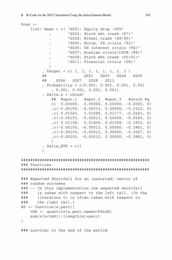
### Scen: Data frame that describes the scenarios## to be added.### The following columns are necessary:### -- Target: 0 or 1 depending on whether### the particular scenario is### included### -- Probability: Probability for this scenario### -- Delta_RTK: Effect of this scenario on the### risk bearing capital RTK)

B R-Code for the SST Calculation Using the delta-Gamma-Model 345

Scen <-list( Name = c( "SZ01: Equity drop -60%"

, "SZ03: Stock mkt crash (87)", "SZ04: Nikkei crash (89/90)", "SZ05: Europ. FX crisis (92)", "SZ06: US interest crisis (94)", "SZ07: Russian crisis/LTCM (98)", "SZ08: Stock mkt crash (00/01)", "SZ11: Financial crisis (08)")

, Target = c( 1, 1, 1, 1, 1, 1, 1, 1 )## SZ01 SZ03 SZ04 SZ05## SZ06 SZ07 SZ08 SZ11, Probability = c(0.001, 0.001, 0.001, 0.001

, 0.001, 0.001, 0.001, 0.001), Delta.x = rbind(

## #spot.1 #spot.2 #spot.3 #stock #qc( 0.00000, 0.00000, 0.00000, -0.6000, 0),c(-0.00155, -0.00013, 0.00000, -0.2323, 0),c( 0.01563, 0.01098, 0.01177, -0.2643, 0),c(-0.00155, -0.00013, 0.00000, -0.0580, 0),c( 0.01109, 0.01406, 0.01509, -0.1852, 0),c(-0.00155, -0.00013, 0.00000, -0.2841, 0),c(-0.00155, -0.00013, 0.00000, -0.3567, 0),c(-0.00155, -0.00013, 0.00000, -0.3881, 0))

, Delta_RTK = c())

########################################################## Functions#######################################################

### Expected Shortfall for an (unsorted) vector of### random outcomes### -- In this implementation the expected shortfall### is taken with respect to the left tail. (In the### literature it is often taken with respect to### the right tail.)ES <- function(x,perc){

VaR <- quantile(x,perc,names=FALSE)sum(x[x<VaR])/(length(x)*perc)

}

### survival to the end of the period


Survival <- function(q) cumprod(1-q)

### discount to the beginning of the first periodDiscount <-function(s) 1/(1+s)^(1:length(s))

### valuation of government bondsbond.gov.value <- function(ZB,date,s){

T <- length(s)if (length(s) != length(ZB)){

return(NA)}else{

return( sum(Discount(s)[date:T]*ZB[date:T])/ if (date == 1) 1else Discount(s)[date-1])

}}

# risk bearing capital at the beginning of period "year"value.assets <- function(x,year){return( bond.gov.value( assets.bond.gov.chf

, year, x[i.spot.chf])

+ (1+stock.chf.incr)^(year-1)

* assets.stock.chf

* x[i.stock.chf])

}

### valuation of insurance polices### -- only survival benefit### -- observe that we do not condition on the### policyholder’s being alive at time year.value.liabilities <- function(x,year){

T <- length(IS)return( sum(Discount(x[i.spot.chf])[year:T]

* Survival(x[i.q]*q)[year:T]

* IS[year:T])

/ if (year == 1) 1else Discount(x[i.spot.chf])[year-1])

}


RTK <- function(x, year){return( value.assets(x,year)

- value.liabilities(x,year) )}

### positive sensitivity for component i of the### risk factors xx.up <- function(x,h,additive,i){

if (additive[i]) x[i] <- x[i]+h[i]else x[i] <- x[i] * (1+h[i])return(x)

}### negative sensitivity for component i of the### risk factors xx.down <- function(x,h,additive,i){

if (additive[i]) x[i] <- x[i]-h[i]else x[i] <- x[i] * (1-h[i])return(x)

}

### Correction for the fact that some sensitivities### are multiplicativeDelta <- function(x,h,additive){

Delta.x <- NULLfor (i in 1:length(x)){

if (additive[i]) Delta.x[i] <- h[i]else Delta.x[i] <- x[i] * h[i]

}return(Delta.x)

}

quad.approx <- function(x, D.RTK, DD.RTK){return(t(x) %*% D.RTK + 0.5*t(x) %*% DD.RTK %*% x)

}

rand.Delta.RTK <- function(N, risk.index){Cov <- ( SD[risk.index] %*% t(SD[risk.index])

* Corr[risk.index, risk.index])

return( apply( rmvnorm( N, rep(0,length(risk.index)), Cov)

, 1


, quad.approx, D.RTK = delta[risk.index], DD.RTK =Gamma[risk.index,risk.index])

)}

### Aggr.Scen: Aggregate Scenarios to randomly### generated values rand### -- We use the same approximation as in the shift### method, namely, two different scenarios cannot### happen in the same year.Aggr.Scen <- function(rand,Scen){

## rand: random values for the distribution## without added scenarios## Scen: Data frame that describes the scenarios## to be added.N.Scen <- length(Scen$Delta_RTK)N.rand <- length(rand)k <- 0for (j in 1:N.Scen){

N.Adjust <- floor( N.rand

* Scen$Target[j]

* Scen$Probability[j])

if (N.Adjust>0){for (l in 1:N.Adjust){

rand[k+l] <-( rand[k+l]+ min(0, Scen$Delta_RTK[j]))

}k <- k+N.Adjust

}}return(rand)

}

########################################################## Calculations#######################################################

### Risk factors, sensitivities, and indicators whether### the sensitivity is additive


x <- NULLh <- NULLadditive <- NULLi.spot.chf <- (length(x)+1):( length(x)

+length(return.spot.chf))h <- c(h, rep(0.01,length(i.spot.chf)))additive <- c(additive, rep(TRUE,length(i.spot.chf)))x <- c(x,return.spot.chf)i.stock.chf <- (length(x)+1):(length(x)+1)h <- c(h,0.1)additive <- c(additive, FALSE)x <- c(x,1)i.q <- (length(x)+1):(length(x)+1)h <- c(h, 0.1)additive <- c(additive, FALSE)x <- c(x,1)

### expected risk bearing capital at the end of period 1### and RTK at the beginning of the projectionRTK.end <- RTK(x,2)RTK.start <- RTK(x,1)

### positive and negative linear sensitivities of the### risk bearing capitald.RTK.plus <- NULLd.RTK.minus <- NULLfor (i in 1:length(x)){d.RTK.plus[i] <- RTK(x.up(x,h,additive,i),2)d.RTK.minus[i] <- RTK(x.down(x,h,additive,i),2)

}

### positive and negative quadratic sensitivities of the### risk bearing capital at the end of period 2dd.RTK.plus.plus <-

matrix( rep(NA,length(x)*length(x)), ncol=length(x))

dd.RTK.plus.minus <-matrix( rep(NA,length(x)*length(x))

, ncol=length(x))

dd.RTK.minus.plus <-matrix( rep(NA,length(x)*length(x))

, ncol=length(x))


dd.RTK.minus.minus <-matrix( rep(NA,length(x)*length(x))

, ncol=length(x))

for (i in 1:length(x)){for (j in 1:length(x)){

dd.RTK.plus.plus[i,j] <-RTK(x.up( x.up( x, h, additive, i)

, h , additive, j), 2)

dd.RTK.plus.minus[i,j] <-RTK(x.up( x.down( x, h, additive, i)

, h, additive, j), 2)

dd.RTK.minus.plus[i,j] <-RTK(x.down( x.up( x, h, additive, i)

, h, additive, j), 2)

dd.RTK.minus.minus[i,j] <-RTK(x.down( x.down( x, h, additive, i)

, h, additive, j),2)}

}

### numerical derivative and second derivative of the## risk bearing capital### at the end of period 2Delta.x <- Delta(x,h,additive)delta <- (d.RTK.plus-d.RTK.minus)/(2*Delta.x)Gamma <- ( dd.RTK.plus.plus - dd.RTK.plus.minus

+ dd.RTK.minus.minus - dd.RTK.minus.plus) / (4 * Delta.x %*% t(Delta.x))

rand.market <-rand.Delta.RTK(N,c(i.spot.chf,i.stock.chf))

rand.insurance <-rand.Delta.RTK(N,c(i.q,i.q))

rand.market.insurance <-rand.Delta.RTK(N,c(i.spot.chf,i.stock.chf, i.q))

for (j in 1:length(Scen$Target)){Scen$Delta_RTK[j] <-

quad.approx(Scen$Delta.x[j,],delta,Gamma)}


rand.market.insurance.scen <-Aggr.Scen(rand.market.insurance, Scen)

risk.capital <-list( insurance = ES(rand.insurance, alpha)

, market = ES(rand.market, alpha), market.insurance =ES(rand.market.insurance, alpha), market.insurance.scen =ES(rand.market.insurance.scen, alpha))

### market value margin for non-hedgeable risks### -- we assume that the following risks are### non-hedgeable:### -- both risk from extreme scenarios and### -- biometric risk is non-hedgeable### -- we assume that the following risks are hedgeable:### -- investment risks for bonds of### duration <= 15 years### -- investment risk for stocks### -- for simplicity we approximate future risk capital### using the market value of liabilities.### This is an approximation.cost.of.capital <- 0for (i in 1:length(IS)){cost.of.capital[i] <-

( coc

* value.liabilities(x,i)/ value.liabilities(x,1)

* ( (risk.capital$market.insurance.scen- risk.capital$market.insurance)

+ risk.capital$insurance))

}MVM <- sum(Discount(return.spot.chf) * cost.of.capital)

### observe that the function RTK already incorporates### expected gainstarget.capital <- ( risk.capital$market.insurance.scen

- return.spot.chf[1] * RTK.start+ MVM) / (1+return.spot.chf[1])


SST.ratio <- -RTK.start/target.capital

########################################################## Output#######################################################

Results <- list()

## placeholder for the 1st entry in ResultsResults$calc_start<- numeric(0)

## placeholder for the 2nd entry in ResultsResults$calc_time_in_s <- numeric(0)

Results$number.simulations <- NResults$alpha <- alphaResults$RTK.start <- RTK.startResults$RTK.end <- RTK.endResults$ES.insurance <- risk.capital$insuranceResults$ES.market <- risk.capital$marketResults$ES.market.insurance <-

risk.capital$market.insuranceResults$ES.market.insurance.scen <-

risk.capital$market.insurance.scenResults$MVM <- MVMResults$target.capital <- target.capitalResults$SST.ratio <- SST.ratiotime.end.user <- proc.time()[["user.self"]]

Results$calc_start <-format(Sys.time(), "%Y-%m-%d_%H:%M:%S")

Results$calc_time_in_s <-time.end.user-time.start.user

print(t(data.frame(Results)))

Appendix CR-Script for the Scenario-Based Solvency IISCR Computation

The computations in Example 4.13 were made with the following script.

tiny <- 1E-6# Our three scenariosBE <- 1UP <- 2DOWN <- 3

# Maturity t, rel. change sup(t), re. change sdown(t)# Durations shorter than 1 year have the same relative# changes as duration 1Shocks <- rbind(c(1, 70/100, -75/100),

c(2, 70/100, -65/100),c(3, 64/100, -56/100),c(4, 59/100, -50/100),c(5, 55/100, -46/100),c(6, 52/100, -42/100),c(7, 49/100, -39/100),c(8, 47/100, -36/100),c(9, 44/100, -33/100),c(10, 42/100, -31/100),c(11, 39/100, -30/100),c(12, 37/100, -29/100),c(13, 35/100, -28/100),c(14, 34/100, -28/100),c(15, 33/100, -27/100),c(16, 31/100, -28/100),c(17, 30/100, -28/100),c(18, 29/100, -28/100),c(19, 27/100, -29/100),c(20, 26/100, -29/100),


353

http://dx.doi.org/10.1007/978-1-4471-6305-3

354 C R-Script for the Scenario-Based Solvency II SCR Computation

c(21, 26/100, -29/100),c(22, 26/100, -30/100),c(23, 26/100, -30/100),c(24, 26/100, -30/100),c(25, 26/100, -30/100),c(30, 25/100, -30/100))

T <- 8

Bonds <- c(1200, 500, 300, 100, 0, 0, 0, 0)Repl <- c( 500, 450, 300, 250, 200, 150, 100, 50)RF_BE <- c( 0.5, 1.0, 1.2, 1.5, 2.0, 2.2, 2.3, 2.3)/100Stat_Interest <- 0.5 / 100

## statutory provisions at the beginning of the period## are equal to the statutory provisions at the end of## the previous periodStatProv_BoP <- vector("numeric",T)for (t in 1:T){StatProv_BoP[t] <-sum( Repl[t:T] / (1+Stat_Interest)^(1:(T-t+1)) )

}

# Initialization of vectors and matricesAssets <- c()Bonus <- matrix(NA,3,T)Liabs <- rep(NA,3)NAV <- rep(NA,3)D_NAV <- rep(NA,3)ADJ_Liabs <- rep(NA,3)ADJ_NAV <- rep(NA,3)ADJ_D_NAV <- rep(NA,3)

# risk free rate for the three scenarios: BE, UP, DOWNRF <- rbind(RF_BE,

RF_BE * (1+Shocks[1:T,UP]),pmax(RF_BE +

pmin(RF_BE * Shocks[1:T,DOWN],-0.01),

0) )

# The policyholders are credited 90% of risk free ratefor (i in c(BE,UP,DOWN)){Bonus[i,] <-

pmax(0, 0.9 * RF[i,] - Stat_Interest) *

C R-Script for the Scenario-Based Solvency II SCR Computation 355

StatProv_BoP}

for (i in c(BE,UP,DOWN)){Assets[i] <- sum(Bonds / cumprod(1+RF[i,]))# Without risk mitigation we use the best estimate# claims in all scenariosLiabs[i] <-sum((Repl+Bonus[BE,]) / cumprod(1+RF[i,]))

NAV[i] <- Assets[i]-Liabs[i]ADJ_Liabs[i] <-sum((Repl+Bonus[i,]) / cumprod(1+RF[i,]))

ADJ_NAV[i] <- Assets[i]-ADJ_Liabs[i]}for (i in c(UP,DOWN)){D_NAV[i] <- max(0,-(NAV[i]-NAV[BE]))ADJ_D_NAV[i] <- max(0,-(ADJ_NAV[i]-ADJ_NAV[BE]))

}

ADJ_SCR <- max(ADJ_D_NAV[UP],ADJ_D_NAV[DOWN],0)

# tiny rather than 0 to avert rounding problemsif (ADJ_SCR < tiny){SCR <- 0

}else if (abs(ADJ_SCR-ADJ_D_NAV[UP]) < tiny){SCR <- D_NAV[UP]

}else{SCR <- D_NAV[DOWN]

}

FDB <- sum(Bonus[BE,]/cumprod(1+RF[BE,]))ADJ <- -min(SCR-ADJ_SCR,FDB)SCR_Final=SCR+ADJ

Results <- data.frame(row.names = c("BE","UP","DOWN"),Assets,Liabs,NAV,D_NAV,ADJ_Liabs,ADJ_NAV,ADJ_D_NAV)

names(Results) = (c("Assets",

356 C R-Script for the Scenario-Based Solvency II SCR Computation

"Liabs","NAV","D_NAV","ADJ_Liabs","ADJ_NAV","ADJ_D_NAV"))

print(round(Results,0))SCR_Result <- data.frame(SCR,ADJ_SCR)names(SCR_Result) <- c("SCR","ADJ_SCR")print(SCR_Result)print(FDB)print(ADJ)print(SCR_Final)

Appendix DR-Script for the Solvency II SCR Computationfor XYZ Inc in Example 4.14

The computation consists in 3 scripts,

D_SII_NL_Input.r, D_SII_NL_Calc.r and D_SII_NL_Output.r,

that are input one after another. The results appear directly in the R console.

D.1 Input Definition

The file D_SII_NL_Input.r defines the input data in Example 4.14:

### Global constantstiny <- 1E-6# gross: before reinsurance, net: after reinsurancegross <- 1; net <- 2

ConfLevel <- 0.995

# Following assignments make indexing more comfortableNoIns <- 3F <- 1 # FireL <- 2 # LiabilityT <- 3 # TheftPY <- 1 # Past YearCY <- 2 # Current YearNY <- 3 # Next Year

Ins_Name <- c("Fire", "Liability", "Theft")Ins_No <- c(

NA, # 1NA, # 2NA, # 3


357

http://dx.doi.org/10.1007/978-1-4471-6305-3

358 D R-Script for the Solvency II SCR Computation for XYZ Inc in Example 4.14

F, # 4L, # 5

NA, # 6NA, # 7NA, # 8T, # 9

NA, # 10NA, # 11NA # 12)

# Row Index: Lob_Name# Column index: Time (PY, CY, NY)

# Gross written premium for PY and CYPrem_written_gross <- rbind(c( 500, 600),

c( 250, 300),c( 50, 100))

# Mean and variation coefficient of the cost per claim# gross of reinsuranceMean_Y_gross <- c(0.1, 0.1, 0.1)VC_Y_gross <- c( 0.5, 0.6, 0.7)

# unearned premiums reserve for PY, CY, NY# (net values)UPR <- rbind(c( 50, 70, 75),

c( 20, 40, 45),c( 5, 12, 15))

#Costs <- c( 0.05, 0.05, 0.05)

# Proportional reinsuranceReP_Q <- c( 0.25, 0.20, 0.20)

# Non-proportional reinsuranceReNP_a <- c( 0.2, 0, 0)ReNP_h <- c( 0.5, 0, 0)

# Reserve patternt_runoff <- 6beta <- array(NA, c(NoIns,t_runoff))beta_temp <- rbind(c(1, 0.6, 0.1, 0.0, 0.0, 0.0),

c(1, 0.9, 0.6, 0.2, 0.1, 0.0),c(1, 0.4, 0.0, 0.0, 0.0, 0.0))

D.1 Input Definition 359

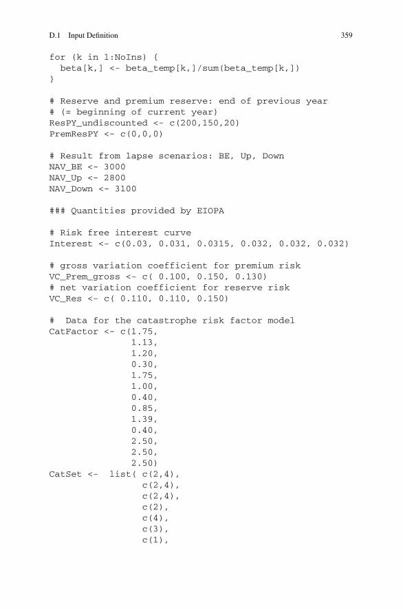
for (k in 1:NoIns) {beta[k,] <- beta_temp[k,]/sum(beta_temp[k,])

}

# Reserve and premium reserve: end of previous year# (= beginning of current year)ResPY_undiscounted <- c(200,150,20)PremResPY <- c(0,0,0)

# Result from lapse scenarios: BE, Up, DownNAV_BE <- 3000NAV_Up <- 2800NAV_Down <- 3100

### Quantities provided by EIOPA

# Risk free interest curveInterest <- c(0.03, 0.031, 0.0315, 0.032, 0.032, 0.032)

# gross variation coefficient for premium riskVC_Prem_gross <- c( 0.100, 0.150, 0.130)# net variation coefficient for reserve riskVC_Res <- c( 0.110, 0.110, 0.150)

# Data for the catastrophe risk factor modelCatFactor <- c(1.75,

1.13,1.20,0.30,1.75,1.00,0.40,0.85,1.39,0.40,2.50,2.50,2.50)

CatSet <- list( c(2,4),c(2,4),c(2,4),c(2),c(4),c(3),c(1),


c(5),c(6),c(9),c(10),c(11),c(12))

# Sets of indices that reflect the structure of# the SCR Cat square root formulaCatSetA <- c(1,2,3,5)CatSetB <- c(11)CatSetC <- c(4,7,8,9,10,12)CatSetD <- c(6,13)

# Event i: 1 2 3 4 5 6# 7 8 9 10 11 12 13CatSplit <- rbind(c(0.1, 0.2, 0.3, 0.0, 0.4, 0.0,

0.0, 0.0, 0.0, 0.0, 0.0, 0.0, 0.0),c(0.0, 0.0, 0.0, 0.0, 0.0, 0.0,

0.0, 1.0, 0.0, 0.0, 0.0, 0.0, 0.0),c(0.0, 0.0, 0.0, 0.0, 0.0, 0.0,

0.0, 0.0, 0.0, 1.0, 0.0, 0.0, 0.0))

# Correlation matrices

# Correlation: premium risk and reserve risk# same correlation for every LoBcorr_PremRes <- rbind(c( 1.0, 0.5),

c( 0.5, 1.0))

# Premium and reserve risk,# correlation: lines of business# F H Dcorr_LoB_LoB <- rbind(c( 1.00, 0.25, 0.50), # F

c( 0.25, 1.00, 0.50), # Hc( 0.50, 0.50, 1.00)) # D

# Correlation: premium/reserve risk and lapse riskcorr_PremRes_Lapse <- rbind(c(1,0),

c(0,1))# Cat risk,# correlation: lines of business# F H Dcorr_Cat <- rbind(c( 1, 0, 0), # F

c( 0, 1, 0), # H

D.2 Computing the SCR 361

c( 0, 0, 1)) # D

# Correlation: premium/reserve/lapse risk and cat riskcorr_PremResLapse_Cat <- rbind(c(1.00, 0.25),

c(0.25, 1.00))

D.2 Computing the SCR

The file D_SII_NL_Calc.r contains the actual computation:

## Earned PremiumPrem <- array(NA, c(NoIns,2))Prem_written<- array(NA, c(NoIns,2))for (t in PY:CY){Prem_written[,t] <- (1-ReP_Q)*Prem_written_gross[,t]Prem[,t] <- Prem_written[,t]+UPR[,t]-UPR[,t+1]

}

# calculation of the variation coefficient# for the net premium risks <- sqrt(log(1 + VC_Y_gross^2))m <- log(Mean_Y_gross) - s^2 / 2

aq <- ReNP_a/(1-ReP_Q)hq <- ReNP_h/(1-ReP_Q)

Mean_Y <-(1-ReP_Q) * ( exp(m+s^2/2) - hq- aq * plnorm(aq,m,s)+ (aq+hq) * plnorm(aq+hq,m,s)+ exp(m+s^2/2)

* plnorm(aq,m+s^2,s)- exp(m+s^2/2)

* plnorm(aq+hq,m+s^2,s))

VC_Y <- sqrt((1-ReP_Q)^2 *((exp(2*m+2*s^2)- 2*hq*exp(m+s^2/2) + hq^2)- aq^2 * plnorm(aq,m,s)+ (aq^2-hq^2) * plnorm(aq+hq,m,s)+ 2*hq*exp(m+s^2/2)

* plnorm(aq+hq,m+s^2,s)+ exp(2*m+2*s^2)


* plnorm(aq,m+2*s^2,s)- exp(2*m+2*s^2)

* plnorm(aq+hq,m+2*s^2,s)) / Mean_Y^2 -1)

VC_Prem <- VC_Prem_gross * sqrt((1+VC_Y^2) / exp(s^2))

#Calculation of volume measured for premium and reserveV_Prem <- c()for (k in 1:NoIns){

V_Prem[k] <- max(Prem_written[k,PY],Prem_written[k,CY],Prem[k,CY])+PremResPY[k]

}

DiscountFactor <- 1V_Res <- array(0,c(NoIns))for (t in 1:t_runoff){

DiscountFactor <- DiscountFactor/(1+Interest[t])V_Res <- ( V_Res +

ResPY_undiscounted

*beta[,t] * DiscountFactor )}

# Calculation of the variation coefficient# for the total premium reserve risksd_Prem <- V_Prem * VC_Premsd_Res <- V_Res * VC_Ressd_PremRes <- c()for (k in 1:NoIns){

sd_PremRes[k] <- sqrt(c(sd_Prem[k],sd_Res[k])%*% corr_PremRes %*%c(sd_Prem[k],sd_Res[k]))

}VC_PremRes <- sd_PremRes / (V_Prem+V_Res)

Mean_PremRes_total <- sum(V_Prem) + sum(V_Res)sd_PremRes_total <- sqrt( sd_PremRes

%*% corr_LoB_LoB %*%sd_PremRes )

VC_PremRes_total <- sd_PremRes_total/Mean_PremRes_total

# Calculation of SCR components and their aggregationSCR_PremRes <- ( Mean_PremRes_total

/ sqrt( 1 + VC_PremRes_total^2 )

D.3 Output from the Computation 363

* exp(sqrt(log(1 + VC_PremRes_total^2))

* qnorm(ConfLevel,0,1)))

SCR_Lapse <- max(NAV_BE-NAV_Up,NAV_BE-NAV_Down)SCR_PremResLapse <- sqrt(c(SCR_PremRes,SCR_Lapse)

%*% corr_PremRes_Lapse %*%c(SCR_PremRes,SCR_Lapse) )

Cat_P_Events <- t(CatSplit) %*% Prem_written_gross[,CY]Cat_Loss <- Cat_P_Events*CatFactorSCR_Cat <- sqrt( (sqrt(sum(Cat_Loss[CatSetA]^2))

+ sum(Cat_Loss[CatSetB]))^2+ sum(Cat_Loss[CatSetC]^2)+ sum(Cat_Loss[CatSetD])^2)

SCR_PremResLapseCat <- sqrt(c(SCR_PremResLapse,SCR_Cat)%*% corr_PremResLapse_Cat %*%c(SCR_PremResLapse,SCR_Cat) )

D.3 Output from the Computation

The most important input quantities and computed values are output to the fileD_SII_NL_Output.r:

print("Company inputs:")dIns <- data.frame(row.names = c("F","L","T"),

Prem_written_gross,UPR,Mean_Y_gross,VC_Y_gross,ReP_Q,ReNP_a,ReNP_h,ResPY_undiscounted,PremResPY)

names(dIns) = (c("Prem_written_gross[,PY]","Prem_written_gross[,CY]","UPR[,PY]","UPR[,CY]","UPR[,NY]","Mean_Y_gross",


"VC_Y_gross","ReP_Q","ReNP_a","ReNP_h","ResPY_undiscounted","PremResPY")

)print(dIns)

dInsCat <- data.frame(row.names = c("F","L","T"),CatSplit)

names(dInsCat) = (c("lambda_1","lambda_2","lambda_3","lambda_4","lambda_5","lambda_6","lambda_7","lambda_8","lambda_9","lambda_10","lambda_11","lambda_12","lambda_13")

)print(dInsCat)

print("")print("Regulatory inputs:")

dEIOPA <- data.frame(row.names = c("F","L","T"),VC_Prem_gross,VC_Res,corr_LoB_LoB)

names(dEIOPA) = (c("VC_Prem_gross","VC_Res","corr_LoB_LoB[,F]","corr_LoB_LoB[,L]","corr_LoB_LoB[,T]")

)print(dEIOPA)

dEIOPACat <- data.frame(CatFactor,t(CatSet))names(dEIOPACat) = (c("CatFactor",

"A_1","A_2","A_3","A_4","A_5","A_6","A_7","A_8","A_9","A_10","A_11","A_12","A_13")

)print(dEIOPACat)

print("");print("Results")

D.3 Output from the Computation 365

dg <- 2

dResults <- data.frame(row.names = c("F","L","T"),round(Prem_written,dg),round(Prem,dg),round(m,dg),round(s,dg),round(Mean_Y,dg+1),round(VC_Y,dg),round(VC_Prem,dg+1),round(V_Prem,dg),round(V_Res,dg),round(sd_Prem,dg),round(sd_Res,dg),round(VC_PremRes,dg+1))

names(dResults) = (c("Prem_written[,PY]","Prem_written[,CY]","Prem[,PY]","Prem[,CY]","m","s","Mean_Y","VC_Y","VC_Prem","V_Prem","V_Res","sd_Prem","sd_Res","VC_PremRes")

)print(dResults)

print(paste("Mean_PremRes_total: ",round(Mean_PremRes_total,dg), sep=""))

print(paste("VC_PremRes_total: ",round(VC_PremRes_total,dg), sep=""))

print(paste("SCR_PremRes: ",round(SCR_PremRes,dg), sep=""))

print(paste("SCR_Lapse: ",round(SCR_Lapse,dg), sep=""))

print(paste("SCR_PremResLapse: ",round(SCR_PremResLapse,dg), sep=""))

print(paste("SCR_Cat: ",


round(SCR_Cat,dg), sep=""))print(paste("SCR_PremResLapseCat: ",

round(SCR_PremResLapseCat,dg), sep=""))

Appendix ER-Script of the Simplified Economic CapitalModel

The computation consists in 3 scripts,

E_EC_Input.r, E_EC_Calc.r and E_EC_Output.r,

that constitute the economic capital model for XYZ Inc. They are input one afteranother. The results appear directly in the R console.

E.1 Input Definition

The file E_EC_Input.r defines the input data from Sect. 7.2.3.1:

# This will give reproducible results:set.seed(2)

### Global constantstiny <- 1E-6# gross: before reinsurance, net: after reinsurancegross <- 1; net <- 2# The BU[[1]] represents Investments# The first insurance BU has therefore index 2FirstIns <- 2

strSep = ",";strDec = ".";

# Global Projection ParametersNoScen <- 10000StartCapital <- 1400FixedCosts <- 20RiskFreeRate <- 0.03ConfLevel <- 0.99


367

http://dx.doi.org/10.1007/978-1-4471-6305-3

368 E R-Script of the Simplified Economic Capital Model

BU_Name <- c( "Investment","Fire","Indemnity","Theft")

BU_Premium <- c( NA, 600, 300, 100)BU_LossRatio <- c( NA, 0.75, 0.75, 0.75)BU_CostRatio <- c( 0.005, 0.05, 0.05, 0.05)BU_VarKoeff <- c( NA, 0.5, 0.6, 0.7)BU_Investments_Mean <- 0.05BU_Investments_Sd <- 0.02BU_ReCeded <- c( 0.00, 0.25, 0.20, 0.20)# Reinsurance commission = negative costs:BU_ReCosts <- c( 0.00, -0.06, -0.06, -0.06)BU_KendalTau <- c( 0.0, 0.0, 0.0, 0.3, 0.2, 0.6)

E.2 Computation of the Economic Capital

The file E_EC_Calc.r contains the actual computation:

require(copula)

NoBU <- length(BU_Name) # Number of business units# including investments

# Structure for all business units, investments# are always BU[[1]]BU <- NULLfor (j in 1:NoBU){# investments: different handling because of# different distributionsif (j==1){tempDistrName <- "norm"tempDistrPar <- list(mean=BU_Investments_Mean,

sd=BU_Investments_Sd)}else{tempDistrName <- "lnorm"tempSdlog <- sqrt(log(1+BU_VarKoeff[j]^2));tempMeanlog <- (log(BU_LossRatio[j]*BU_Premium[j])

-tempSdlog^2/2);tempDistrPar <- list(meanlog=tempMeanlog,

sdlog=tempSdlog)}

E.2 Computation of the Economic Capital 369

NextBU <- list(Name = BU_Name[j],Premium=BU_Premium[j],LossRatio=BU_LossRatio[j],CostRatio = BU_CostRatio[j],Distr = list(Name=tempDistrName,

NoArg = 2,Par = tempDistrPar),

Q = list(Ceded=BU_ReCeded[j],Costs=BU_ReCosts[j]))

BU <- c(BU,list(NextBU))}NextBU <- NULL # Not needed any more

# Set-up of copula using functionality from the# copula packagecop <- normalCopula(param = sin( pi/2 * BU_KendalTau),

dim = NoBU,dispstr = "un");

copMargin <- NULLcopMarginPar <- NULLfor (i in 1:NoBU){

copMargin <- c(copMargin,BU[[i]]$Distr$Name)copMarginPar <- c(copMarginPar,

list(BU[[i]]$Distr$Par))}rDistribution <- rMvdc(NoScen,

mvdc(cop,copMargin,copMarginPar)

)

##### We will now calculate the profit for each run

Profit <- list(BU = array(NA,dim=c(NoScen,NoBU,2)),total = array(NA,dim=c(NoScen,2)),BU.mean = array(NA,dim=c(NoBU,2)),total.mean = array(NA,dim=c(2)))

##### Premium ------------------------------------#Premium <- NULL;# BU index that corresponds to insurance index:bu <- NULL# Insurance index that corresponds to BU index:ins <- NULLfor (j in FirstIns:NoBU){


ins[j] <- j-FirstIns+1bu[ins[j]] <- j

}NoIns <- length(bu)

Premium <- array(NA,dim=c(NoIns,2));for (j in 1:NoIns){Premium[j,gross] <- BU[[bu[j]]]$Premium;Premium[j,net] <- (Premium[j,gross]

* (1-BU[[bu[j]]]$Q$Ceded));}

# Investment assetsAssets <- array(NA,dim=c(2));for (gn in gross:net){Assets[gn] <- StartCapital+sum(Premium[1:NoIns,gn])

}

##### Costs --------------------------------------Costs <- NULL;Costs <- array(NA,dim=c(NoBU,2));

for (gn in gross:net){Costs[1,gn] <- BU[[1]]$CostRatio * Assets[gn];

}for (j in 1:NoIns){for (gn in gross:net){Costs[bu[j],gn] <- (BU[[bu[j]]]$CostRatio

* Premium[j,gross])}Costs[bu[j],net] <- (Costs[bu[j],net]

+ BU[[bu[j]]]$Q$Costs

* (Premium[j,gross]-Premium[j,net]))

}

##### Profit -------------------------------------for (gn in gross:net){# rDistribution[,1] represents the relative# return from the investmentProfit$BU[,1,gn] <- ((rDistribution[,1]

-RiskFreeRate)

*Assets[gn]-Costs[1,gn])}for (j in 1:NoIns){

E.2 Computation of the Economic Capital 371

Profit$BU[,bu[j],gross] <- ((1+RiskFreeRate)

*Premium[j,gross]- rDistribution[,bu[j]]- Costs[bu[j],gross])

Profit$BU[,bu[j],net] <- ((1+RiskFreeRate)

*Premium[j,net]- (1-BU[[bu[j]]]$Q$Ceded)

*rDistribution[,bu[j]]- Costs[bu[j],net])

}for (gn in gross:net){for (j in 1:NoBU){Profit$BU.mean[j,gn] <- (sum(Profit$BU[,j,gn])

/NoScen)}

}

for (gn in gross:net){Profit$total[,gn] <- (RiskFreeRate * StartCapital

- FixedCosts)for (j in 1:NoBU){Profit$total[,gn] <- (Profit$total[,gn]

+ Profit$BU[,j,gn])}Profit$total.mean[gn] <- (sum(Profit$total[,gn])

/NoScen)}

#### We will now calculate the economic capital#### and the risk-adjusted return

EcoCap <- list(BU = array(NA,dim=c(NoBU,2)),total = array(NA,dim=c(1,2)))

RORAC <- list(BU = array(NA,dim=c(NoBU,2)),total = array(NA,dim=c(1,2)))

NotDefined <- -999

ES <- function(profit, perc){# Calculation of the expected shortfallquantiles <- profit[order(profit,c(1:length(profit)),

decreasing=FALSE)]result <- NA;if(!is.na(perc)){


if (0 < perc & perc < 1){result <- sum(quantiles[1:ceiling(

(1-perc)*length(quantiles))])result <- -(result

/ ceiling((1-perc)

*length(quantiles)))}else{warning(paste(" perc should be in ]0,1[,",

" perc = ", perc, sep=""))}

}result

}

### Calculation of all economic capital valuesfor (gn in gross:net){for (j in 1:NoBU){EcoCap$BU[j,gn] <- ES(Profit$BU[,j,gn], ConfLevel)

}EcoCap$total[gn] <- ES(Profit$total[,gn], ConfLevel)

}

### Calculation of all RAROC valuesfor (gn in gross:net){for (j in 1:NoBU){if (EcoCap$BU[j,gn] <= tiny){RORAC$BU[j,gn] <- NotDefined

}else{RORAC$BU[j,gn] <- (Profit$BU.mean[j,gn]

/EcoCap$BU[j,gn])}

}if (EcoCap$total[gn] <= tiny){RORAC$total[gn] <- NotDefined

}else{RORAC$total[gn] <- (Profit$total.mean[gn]

/EcoCap$total[gn])}

}

E.3 Output from the Computation

The expected return, economic capital and RORAC are output to E_EC_Output.r:

E.3 Output from the Computation 373

# Check that it works:print("Order of business units:")for (j in 1:NoBU){print(paste(j, ": ", BU[[j]]$Name, sep=""))

}print(paste("Gross: ", gross,

", Net ", net, sep=""))

print("Profit of business units: ")print(Profit$BU.mean)print("Total profit:")print(Profit$total.mean)

print("Economic capital for business units: ")print(EcoCap$BU)print("Total economic capital:")print(EcoCap$total)

print("RORAC for business units: ")print(RORAC$BU)print("Total RORAC:")print(RORAC$total)

Index

Symbols� (measures), 26MB(Ω,Rk), 17M (Ω,Rk), 17R̄, 75t -fiber, 50

AAbsolutely continuous, 26Allocation

capital, 285resources, 274

Allotment, 200discrete, 209dominates, 209global, 227

continuous, 228ALM, 284Asset liability management, 254

BBalanced scorecard, 280Best estimate, 114Black box, 285Bonus

administration, 304claims acceptance, 304imputed, 303marketing, 304performance-dependent, 303product pricing, 304sales, 303underwriting, 303

BSC, 280Business area, 197Business areas segmentation, 197

CCapital

allocated, 199allocation, 199available, 107contribution, 211economic, 108excess, 199profit-participation rights, 323proportional allocation, 201risk-bearing, 107value based, 260

Capital allocation, 199, 279Aumann-Shapley, 221covariance, 207Euler, 206global, 225

continuous, 228marginal

continuous, 205discrete, 202

proportional, 201Capital market line, 336Capital market model

Hull-White, 284Capital model

economic, 285Cash flow, 250

deterministic, 250insurance, 251

pure, 251value, 252

deterministic, 255market consistent, 266

value process, 255Certificates

profit-sharing, 323


375

http://dx.doi.org/10.1007/978-1-4471-6305-3

376 Index

Claims basis, 321Company

protecting, 274strategy, 277value

market consistent, 250Comparison consistent, 69Confidence level, 18Continuation

insurance company, 319Copula, 76

Gauss, 87Gaussian, 287Gumbel, 91independence, 94

Correlationlinear, 84, 99

Cost accounting, 238Cost of capital, 104, 241Costs, 238

cost unit, 238direct, 238fixed, 238full-cost accounting, 238partial-cost accounting, 238variable, 238, 239

DDiagram

risk-return, 336Distribution

compound Poisson, 296lognormal, 286normal, 286

Distribution strategies, 307Diversification, 73, 285Division view, 283, 301

EEconomic value added, 241Efficient frontier, 292, 336Embedded value

market consistent, 261Enterprise risk management, 271Equity capital, 323Equity character, 323ERM, 271

Committee, 276Euclidean space, 34Euler’s principle, 206EVA, 239, 241

value based, 260Excess capital, 108, 199Expectation

conditional, 46Expected shortfall, 22, 285

dynamic, 56

FFair value, 113Feedback effect, 130Filtration, 45

product, 49Financial market stability, 319FINMA, 131Function aspect, 283Function view, 302

GGoing-concern, 111, 319Governance, 276Guarantee funds, 321

HHidden reserves, 324Hierarchy level, 279Hurdle rate, 240, 279

IInfimum

essential, 57Insolvency, 107Interest costs, 241Investment

risk-free, 335risky, 335

Investors, 271Isometry, 34

KKendall’s τ , 86Key performance indicator, 267Key risk indicator, 274KonTraG, 314KRI, 274, 276

LLiabilities

subordinated, 323Liquidity risk, 284

MManagement

measurement component, 274organizational component, 276, 305process component, 277, 307strategic component, 272

Map transpose, 34Marginal dependence, 95

Index 377

Marginal distribution, 75MaRisk, 330Market portfolio, 338Market value margin, 115Martingale, 263Maximal losses, 298Model

analytic, 126factor-based, 125Monte Carlo, 129reinsurance, 129scenario-based, 126

Modelingevolution continuous, 295limitations, 295

MVM, 115

NNet profit after tax, 240Newton method, 131Nominal results, 243Nominal value, 243Normal distribution assumption of, 126

OOpportunity costs, 104Optimization

iterative process, 295reinsurance, 292

Optimizingproduct mix, 292

Orthogonal, 34

PPartition, 45Performance measurement, 237Perspective

customer, 280financial, 280internal business processes, 280learning and growth, 280

Portfolio, 335normed, 335pure, 335

Predistribution function, 75Premium refunds

free, 324Price

risk-adjusted, 290Price setting, 274Process

stochasticpredictable, 264previsible, 264

Product economyfiltered, 51

Profit center, 283Profit measurement, 238

RRandom variable

elliptical, 36spherical, 36

RAROC, 242Rating, 130Rating agencies, 277Rating companies, 272Reference company, 111Reinsurance contract

non-proportional, 130Retrocession, 130Return on capital, 242Return on risk adjusted capital, 243RfB

free, 324Risk

appetite, 272, 279aversion, 103capital, 1, 17, 124

economic, 108operationally necessary, 110

context, 108handbook, 317hedgeable, 115, 261indicator, 277, 317limit, 317liquidity, 275map, 317matrix, 317mitigation measure, 317neutral, 267non-hedgeable, 115, 261operational, 275premium, 341recording forms, 317register, 317report, 305strategic, 275strategy, 277tolerance, 272trend, 275

Risk adjusted return on capital, 242Risk and capital management, 271Risk free interest curve, 132Risk measure, 17

coherent, 31convex, 32discrete, 209

378 Index

Risk measure (cont.)subadditive, 209

dynamic, 54comparison consistent, 69time-consistent, 58weakly time-consistent, 58

dynamic coherent, 54monotony, 31positive homogeneity, 31subadditivity, 31translation invariance, 31

ROC, 242RORAC, 243, 288

value based, 260Run-off, 110, 319

SSafety buffer fluctuations, 291Safety level, 18Scenario

historical, 127hypothetical, 127multiple, 127single, 127standard, 127

Segmentation induced volume parametrization,204

Shapley algorithm, 211Share capital, 324Shareholder value, 253σ -algebra product, 47Sklar, 78Solvency guidelines, 274, 277Solvency I, 122, 125, 319Solvency II, 122, 170, 325Solvency margin, 318Solvency requirements, 318Solvent, 107Spearman’s rho, 84Spectral measure, 30Spread, 104SST, 131

δ-Γ -model, 134loss function, 133market value margin, 133risk capital, 133risk-bearing capital (RTK), 132target capital, 133

Standard ModelSST, 131

Stochastic process, 45Strategy, 280Supervisors, 271Supremum

essential, 57, 64Swiss Solvency Test, see SSTSynergies, 250

TTail dependence, 95Tail value at risk, 22Target rating, 274Theorem

copula invariance, 81Time-consistent, 58

weakly, 58Trading strategy

self-financing, 264Trend risk, 284

VValuation

entity method, 254equity method, 253market consistent, 261stakeholder method, 254

Value, 252creation, 242destruction, 242deterministi, 255process, 255

Value at risk, 20dynamic, 55

Value based management, 271VaR, 20VBM, 271Vision, 280Volume parametrization, 205

induced, 204

WWeight function, 30World

real, 267risk neutral, 267

Appendix A The Capital Asset Pricing Model (CAPM)978-1-4471-6305...Appendix A The Capital Asset...

Documents

Transcript of Appendix A The Capital Asset Pricing Model (CAPM)978-1-4471-6305...Appendix A The Capital Asset...