APPENDIX A MODELING REPORT - Pinellas County, …...COASTAL PLANNING & ENGINEERING, INC. UPHAM BEACH...

COASTAL PLANNING & ENGINEERING, INC.

APPENDIX A

MODELING REPORT

i COASTAL PLANNING & ENGINEERING, INC.

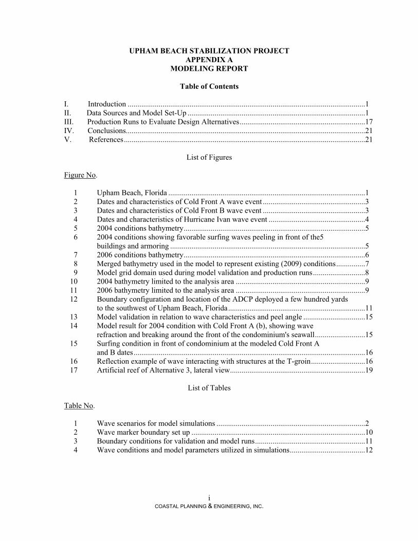
UPHAM BEACH STABILIZATION PROJECT APPENDIX A

MODELING REPORT

Table of Contents I. Introduction ...........................................................................................................................1 II. Data Sources and Model Set-Up ............................................................................................1 III. Production Runs to Evaluate Design Alternatives .................................................................17 IV. Conclusions............................................................................................................................21 V. References .............................................................................................................................21

List of Figures

Figure No. 1 Upham Beach, Florida ......................................................................................................1 2 Dates and characteristics of Cold Front A wave event .....................................................3 3 Dates and characteristics of Cold Front B wave event .....................................................3 4 Dates and characteristics of Hurricane Ivan wave event ..................................................4 5 2004 conditions bathymetry ..............................................................................................5 6 2004 conditions showing favorable surfing waves peeling in front of the5 buildings and armoring .....................................................................................................5 7 2006 conditions bathymetry ..............................................................................................6 8 Merged bathymetry used in the model to represent existing (2009) conditions ...............7 9 Model grid domain used during model validation and production runs ...........................8 10 2004 bathymetry limited to the analysis area ...................................................................9 11 2006 bathymetry limited to the analysis area ...................................................................9 12 Boundary configuration and location of the ADCP deployed a few hundred yards to the southwest of Upham Beach, Florida .......................................................................11 13 Model validation in relation to wave characteristics and peel angle ................................15 14 Model result for 2004 condition with Cold Front A (b), showing wave refraction and breaking around the front of the condominium's seawall ..........................15 15 Surfing condition in front of condominium at the modeled Cold Front A and B dates ........................................................................................................................16 16 Reflection example of wave interacting with structures at the T-groin ............................16 17 Artificial reef of Alternative 3, lateral view ......................................................................19

List of Tables

Table No. 1 Wave scenarios for model simulations .............................................................................2 2 Wave marker boundary set up ..........................................................................................10 3 Boundary conditions for validation and model runs .........................................................11 4 Wave conditions and model parameters utilized in simulations .......................................12

1 COASTAL PLANNING & ENGINEERING, INC.

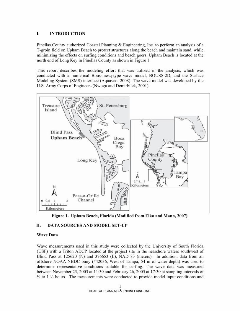
I. INTRODUCTION Pinellas County authorized Coastal Planning & Engineering, Inc. to perform an analysis of a T-groin field on Upham Beach to protect structures along the beach and maintain sand, while minimizing the effects on surfing conditions and beach goers. Upham Beach is located at the north end of Long Key in Pinellas County as shown in Figure 1. This report describes the modeling effort that was utilized in the analysis, which was conducted with a numerical Boussinesq-type wave model, BOUSS-2D, and the Surface Modeling System (SMS) interface (Aquaveo, 2008). The wave model was developed by the U.S. Army Corps of Engineers (Nwogu and Demirbilek, 2001).

Figure 1. Upham Beach, Florida (Modified from Elko and Mann, 2007).

II. DATA SOURCES AND MODEL SET-UP

Wave Data Wave measurements used in this study were collected by the University of South Florida (USF) with a Triton ADCP located at the project site in the nearshore waters southwest of Blind Pass at 125620 (N) and 376653 (E), NAD 83 (meters). In addition, data from an offshore NOAA-NBDC buoy (#42036, West of Tampa, 54 m of water depth) was used to determine representative conditions suitable for surfing. The wave data was measured between November 23, 2003 at 11:30 and February 26, 2005 at 17:30 at sampling intervals of ½ to 1 ½ hours. The measurements were conducted to provide model input conditions and


model validation information. The location of the instrument is described further in the discussion of boundary conditions in a later section of this report. The wave data was provided as statistical wave parameters, significant wave height, peak wave period, peak wave direction, peak spreading, and mean direction (see Appendix A-1). Due to bio-fouling of the USF equipment, the directional wave measurements were not reliable. Even though directional measurements were interrupted, wave height and period measurements were still valid since the sensors were able to measure pressure variations after burial. In place of the unreliable data, directional data from the offshore NOAA buoy was used to select three wave events from the dataset to conduct model validation and production runs (Table 1).

Table 1. Wave scenarios for model simulations.

WAVE SCENARIOS

EVENT Hs (m/ft) Tp (s) Nearshore Direction (degrees)

Cold Front A 0.75/2.5 9.2 270

Cold Front A (b) * 0.75/2.5 9.2 290

Cold Front B 0.9/3.0 6.5 282

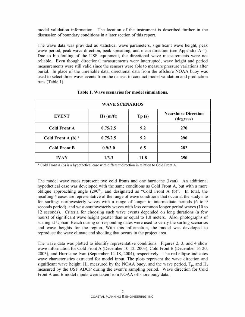
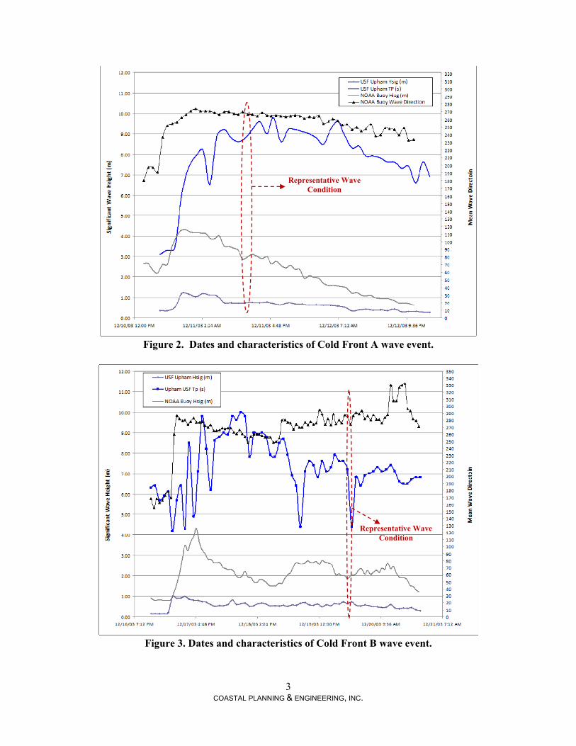
IVAN 1/3.3 11.8 250 * Cold Front A (b) is a hypothetical case with different direction in relation to Cold Front A. The model wave cases represent two cold fronts and one hurricane (Ivan). An additional hypothetical case was developed with the same conditions as Cold Front A, but with a more oblique approaching angle (290o), and designated as “Cold Front A (b)”. In total, the resulting 4 cases are representative of the range of wave conditions that occur at the study site for surfing: northwesterly waves with a range of longer to intermediate periods (6 to 9 seconds period), and west-southwesterly waves with less common longer period waves (10 to 12 seconds). Criteria for choosing such wave events depended on long durations (a few hours) of significant wave height greater than or equal to 1.0 meters. Also, photographs of surfing at Upham Beach during corresponding dates were used to verify the surfing scenarios and wave heights for the region. With this information, the model was developed to reproduce the wave climate and shoaling that occurs in the project area. The wave data was plotted to identify representative conditions. Figures 2, 3, and 4 show wave information for Cold Front A (December 10-12, 2003), Cold Front B (December 16-20, 2003), and Hurricane Ivan (September 14-18, 2004), respectively. The red ellipse indicates wave characteristics extracted for model input. The plots represent the wave direction and significant wave height, Hs, measured by the NOAA buoy, and the wave period, Tp, and Hs measured by the USF ADCP during the event’s sampling period. Wave direction for Cold Front A and B model inputs were taken from NOAA offshore buoy data.


Figure 2. Dates and characteristics of Cold Front A wave event.

Figure 3. Dates and characteristics of Cold Front B wave event.

Representative Wave Condition



Figure 4. Dates and characteristics of Hurricane Ivan wave event.

Bathymetry Data

Model Validation Bathymetry Multiple sources of bathymetric data were integrated for this study. For model validation, two bathymetric scenarios were considered:

1. The 2004 bathymetry represents conditions before the geotextile T-groins placement, characterized by USACE 2004 LIDAR data;

2. The 2006 bathymetry, representing conditions after placement of the geotextile T-groins, characterized by Post Wilma 2006 LIDAR data.

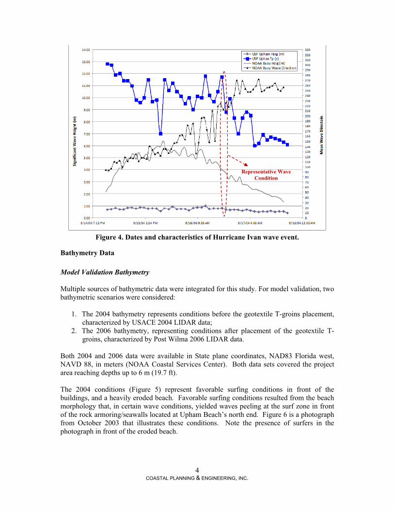
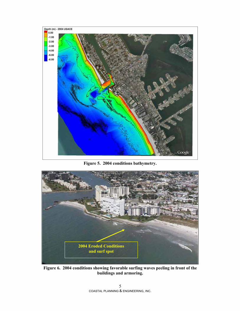
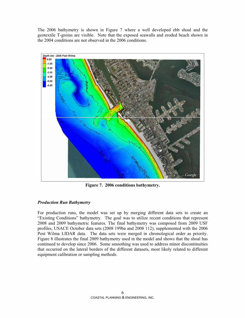
Both 2004 and 2006 data were available in State plane coordinates, NAD83 Florida west, NAVD 88, in meters (NOAA Coastal Services Center). Both data sets covered the project area reaching depths up to 6 m (19.7 ft). The 2004 conditions (Figure 5) represent favorable surfing conditions in front of the buildings, and a heavily eroded beach. Favorable surfing conditions resulted from the beach morphology that, in certain wave conditions, yielded waves peeling at the surf zone in front of the rock armoring/seawalls located at Upham Beach’s north end. Figure 6 is a photograph from October 2003 that illustrates these conditions. Note the presence of surfers in the photograph in front of the eroded beach.



Figure 5. 2004 conditions bathymetry.

Figure 6. 2004 conditions showing favorable surfing waves peeling in front of the

buildings and armoring.

2004 Eroded Conditions and surf spot


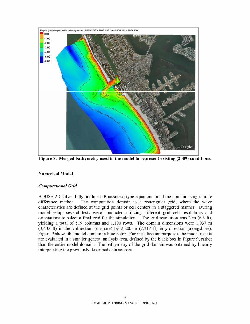
The 2006 bathymetry is shown in Figure 7 where a well developed ebb shoal and the geotextile T-groins are visible. Note that the exposed seawalls and eroded beach shown in the 2004 conditions are not observed in the 2006 conditions.

Figure 7. 2006 conditions bathymetry.

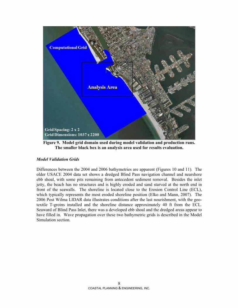
Production Run Bathymetry For production runs, the model was set up by merging different data sets to create an “Existing Conditions” bathymetry. The goal was to utilize recent conditions that represent 2008 and 2009 bathymetric features. The final bathymetry was composed from 2009 USF profiles, USACE October data sets (2008 199ba and 2008 112), supplemented with the 2006 Post Wilma LIDAR data. The data sets were merged in chronological order as priority. Figure 8 illustrates the final 2009 bathymetry used in the model and shows that the shoal has continued to develop since 2006. Some smoothing was used to address minor discontinuities that occurred on the lateral borders of the different datasets, most likely related to different equipment calibration or sampling methods.


Figure 8. Merged bathymetry used in the model to represent existing (2009) conditions.

Numerical Model

Computational Grid BOUSS-2D solves fully nonlinear Boussinesq-type equations in a time domain using a finite difference method. The computation domain is a rectangular grid, where the wave characteristics are defined at the grid points or cell centers in a staggered manner. During model setup, several tests were conducted utilizing different grid cell resolutions and orientations to select a final grid for the simulations. The grid resolution was 2 m (6.6 ft), yielding a total of 519 columns and 1,100 rows. The domain dimensions were 1,037 m (3,402 ft) in the x-direction (onshore) by 2,200 m (7,217 ft) in y-direction (alongshore). Figure 9 shows the model domain in blue color. For visualization purposes, the model results are evaluated in a smaller general analysis area, defined by the black box in Figure 9, rather than the entire model domain. The bathymetry of the grid domain was obtained by linearly interpolating the previously described data sources.


Figure 9. Model grid domain used during model validation and production runs.

The smaller black box is an analysis area used for results evaluation.

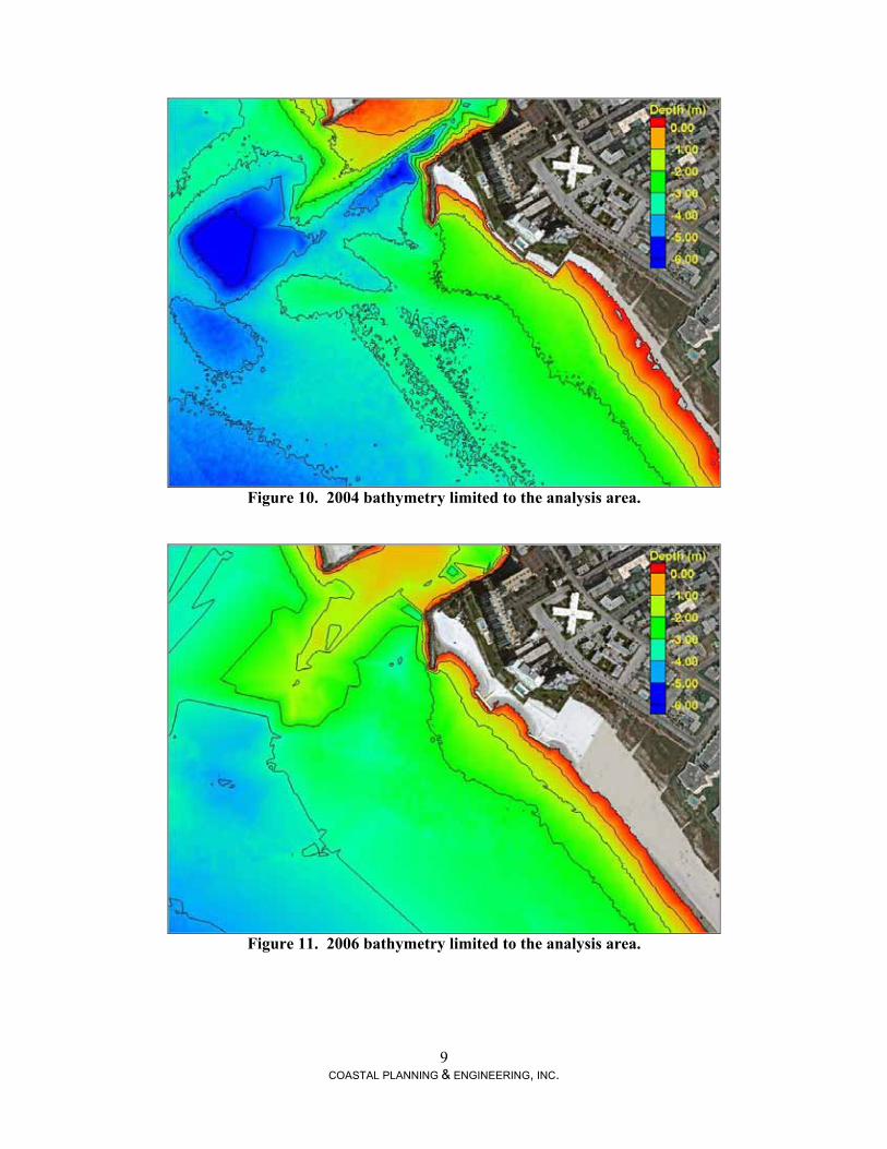
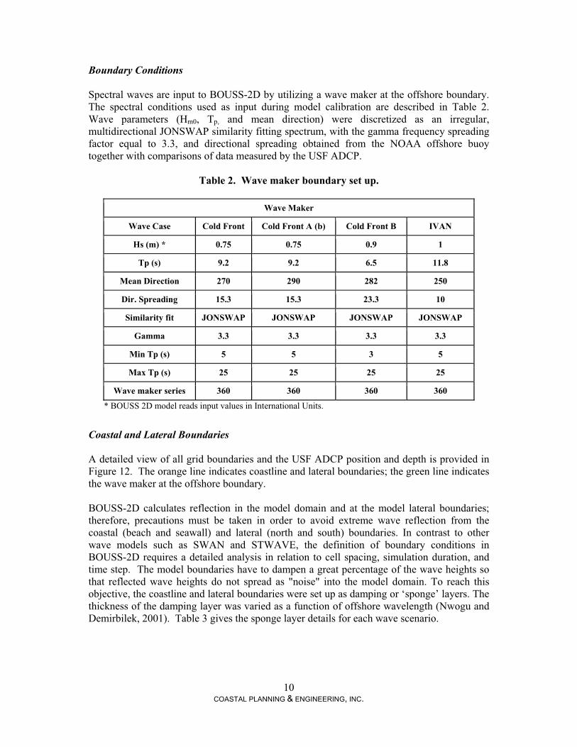
Model Validation Grids Differences between the 2004 and 2006 bathymetries are apparent (Figures 10 and 11). The older USACE 2004 data set shows a dredged Blind Pass navigation channel and nearshore ebb shoal, with some pits remaining from antecedent sediment removal. Besides the inlet jetty, the beach has no structures and is highly eroded and sand starved at the north end in front of the seawalls. The shoreline is located close to the Erosion Control Line (ECL), which typically represents the most eroded shoreline position (Elko and Mann, 2007). The 2006 Post Wilma LIDAR data illustrates conditions after the last nourishment, with the geo-textile T-groins installed and the shoreline distance approximately 40 ft from the ECL. Seaward of Blind Pass Inlet, there was a developed ebb shoal and the dredged areas appear to have filled in. Wave propagation over these two bathymetric grids is described in the Model Simulation section.


Figure 10. 2004 bathymetry limited to the analysis area.

Figure 11. 2006 bathymetry limited to the analysis area.


Boundary Conditions Spectral waves are input to BOUSS-2D by utilizing a wave maker at the offshore boundary. The spectral conditions used as input during model calibration are described in Table 2. Wave parameters (Hm0, Tp, and mean direction) were discretized as an irregular, multidirectional JONSWAP similarity fitting spectrum, with the gamma frequency spreading factor equal to 3.3, and directional spreading obtained from the NOAA offshore buoy together with comparisons of data measured by the USF ADCP.

Table 2. Wave maker boundary set up.

Wave Maker

Wave Case Cold Front Cold Front A (b) Cold Front B IVAN

Hs (m) * 0.75 0.75 0.9 1

Tp (s) 9.2 9.2 6.5 11.8

Mean Direction 270 290 282 250

Dir. Spreading 15.3 15.3 23.3 10

Similarity fit JONSWAP JONSWAP JONSWAP JONSWAP

Gamma 3.3 3.3 3.3 3.3

Min Tp (s) 5 5 3 5

Max Tp (s) 25 25 25 25

Wave maker series 360 360 360 360

* BOUSS 2D model reads input values in International Units.

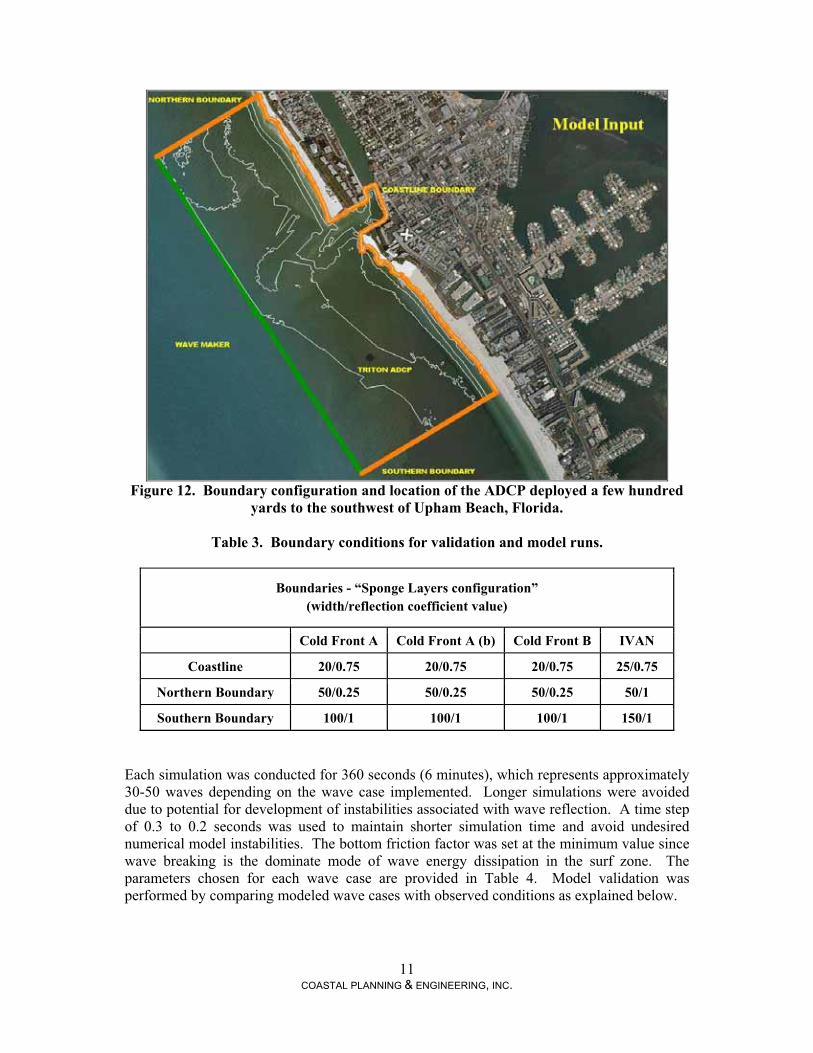
Coastal and Lateral Boundaries A detailed view of all grid boundaries and the USF ADCP position and depth is provided in Figure 12. The orange line indicates coastline and lateral boundaries; the green line indicates the wave maker at the offshore boundary. BOUSS-2D calculates reflection in the model domain and at the model lateral boundaries; therefore, precautions must be taken in order to avoid extreme wave reflection from the coastal (beach and seawall) and lateral (north and south) boundaries. In contrast to other wave models such as SWAN and STWAVE, the definition of boundary conditions in BOUSS-2D requires a detailed analysis in relation to cell spacing, simulation duration, and time step. The model boundaries have to dampen a great percentage of the wave heights so that reflected wave heights do not spread as "noise" into the model domain. To reach this objective, the coastline and lateral boundaries were set up as damping or ‘sponge’ layers. The thickness of the damping layer was varied as a function of offshore wavelength (Nwogu and Demirbilek, 2001). Table 3 gives the sponge layer details for each wave scenario.


Figure 12. Boundary configuration and location of the ADCP deployed a few hundred

yards to the southwest of Upham Beach, Florida.

Table 3. Boundary conditions for validation and model runs.

Boundaries - “Sponge Layers configuration” (width/reflection coefficient value)

Cold Front A Cold Front A (b) Cold Front B IVAN

Coastline 20/0.75 20/0.75 20/0.75 25/0.75

Northern Boundary 50/0.25 50/0.25 50/0.25 50/1

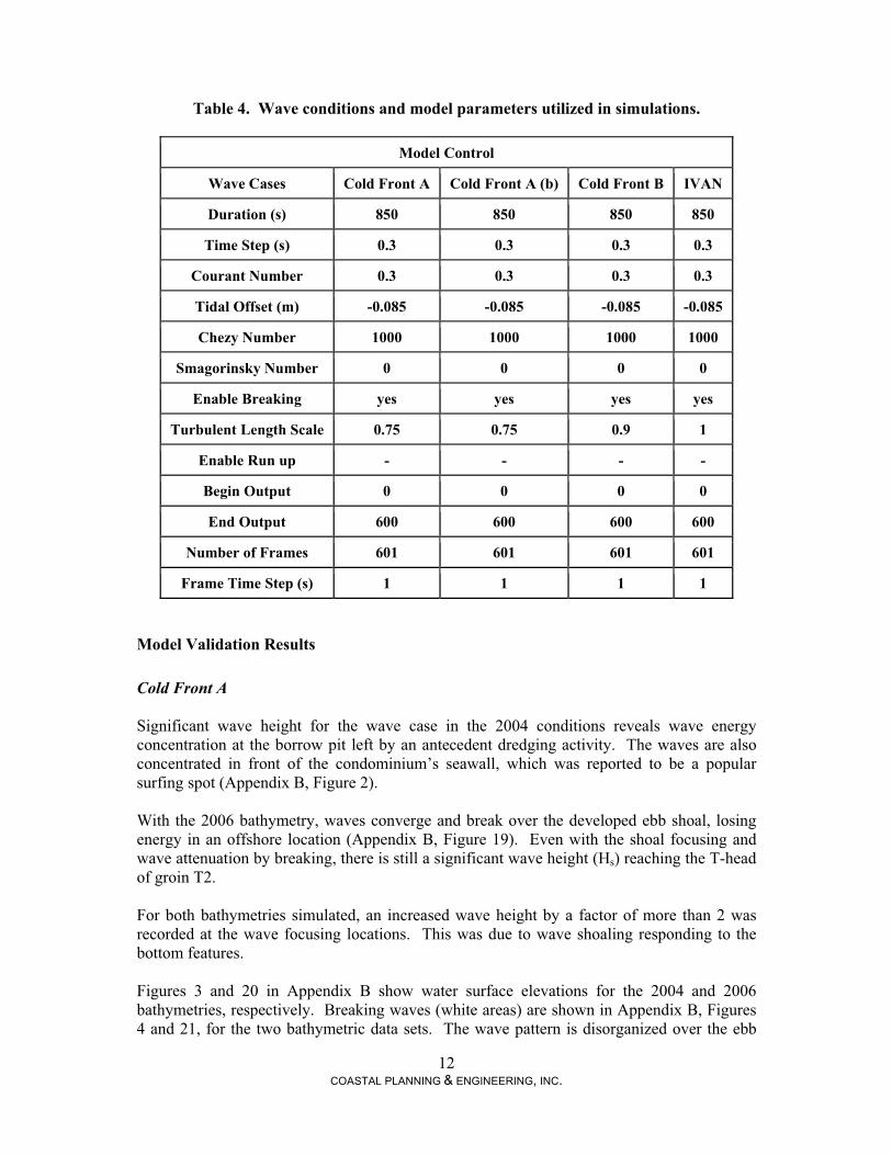
Southern Boundary 100/1 100/1 100/1 150/1 Each simulation was conducted for 360 seconds (6 minutes), which represents approximately 30-50 waves depending on the wave case implemented. Longer simulations were avoided due to potential for development of instabilities associated with wave reflection. A time step of 0.3 to 0.2 seconds was used to maintain shorter simulation time and avoid undesired numerical model instabilities. The bottom friction factor was set at the minimum value since wave breaking is the dominate mode of wave energy dissipation in the surf zone. The parameters chosen for each wave case are provided in Table 4. Model validation was performed by comparing modeled wave cases with observed conditions as explained below.


Table 4. Wave conditions and model parameters utilized in simulations.

Model Control

Wave Cases Cold Front A Cold Front A (b) Cold Front B IVAN

Duration (s) 850 850 850 850

Time Step (s) 0.3 0.3 0.3 0.3

Courant Number 0.3 0.3 0.3 0.3

Tidal Offset (m) -0.085 -0.085 -0.085 -0.085

Chezy Number 1000 1000 1000 1000

Smagorinsky Number 0 0 0 0

Enable Breaking yes yes yes yes

Turbulent Length Scale 0.75 0.75 0.9 1

Enable Run up - - - -

Begin Output 0 0 0 0

End Output 600 600 600 600

Number of Frames 601 601 601 601

Frame Time Step (s) 1 1 1 1

Model Validation Results

Cold Front A Significant wave height for the wave case in the 2004 conditions reveals wave energy concentration at the borrow pit left by an antecedent dredging activity. The waves are also concentrated in front of the condominium’s seawall, which was reported to be a popular surfing spot (Appendix B, Figure 2). With the 2006 bathymetry, waves converge and break over the developed ebb shoal, losing energy in an offshore location (Appendix B, Figure 19). Even with the shoal focusing and wave attenuation by breaking, there is still a significant wave height (Hs) reaching the T-head of groin T2. For both bathymetries simulated, an increased wave height by a factor of more than 2 was recorded at the wave focusing locations. This was due to wave shoaling responding to the bottom features. Figures 3 and 20 in Appendix B show water surface elevations for the 2004 and 2006 bathymetries, respectively. Breaking waves (white areas) are shown in Appendix B, Figures 4 and 21, for the two bathymetric data sets. The wave pattern is disorganized over the ebb


shoal in the 2006 conditions, with crossing wave crests due to refraction over the shoal and also some reflection from the jetty. Figures 5 and 22 in Appendix B show the surface current patterns. Figure 5, representing 2004 conditions, showed greater alongshore currents, with maximum values of 1.64 m/s, while 2006 conditions revealed less intense currents due to the wave breaking over the ebb shoal in combination with the geotube T-groins.

Cold Front A (b) Cold Front A (b) uses the conditions from Cold Front A with a higher approaching angle relative to the shore. Significant wave height, water surface elevation, wave breaking, and current pattern results for both bathymetries can be found in Appendix B, Figures 6-9 and 23-26. For the 2004 condition, larger wave heights are focused more seaward of the ebb shoal than in Cold Front A conditions (Figure 6, Appendix B). Significant wave height in front of the buildings is also smaller, but high wave crests are propagating around the end of the building’s seawall (Figure 7, Appendix B). Overall, wave energy is shifted towards offshore and more waves are propagating and reaching the beach much further down the coast (Figures 6-9, Appendix B). For the 2006 bathymetry, waves are shoaling and breaking over the developed ebb shoal (Figure 23, Appendix B). Compared to Cold Front A conditions, wave focusing is located seaward, wave height is smaller, and the majority of the larger waves are reaching the shore at the first T-head groin (Figures 23-24, Appendix B). A disorganized wave pattern over the ebb shoal also occurs, with crossing wave crests due to shoal-induced refraction and reflection caused by the jetty (similar to Cold Front A). For this wave case (in both bathymetric conditions), an increased wave height by a factor of about 2 occurred at the wave focusing locations, similar to Cold Front A. Nearshore surface current patterns for 2004 conditions were more intense and concentrated alongshore, while currents for the 2006 conditions were less intense. This is a similar observation as in Cold Front A, due to wave breaking over the ebb shoal acting together with the geotube T-groins (Figures 9 and 26).

Cold Front B Cold Front B was characterized by shorter period waves (6.5 s) with higher Hs (0.9 m/2.95 ft), and a more oblique wave approach in relation to the other wave cases. Significant wave height, water surface elevation, wave breaking, and current pattern results for both bathymetries can be found in Appendix B, Figures 10-13 and 27-30. Significant wave height over the 2004 bathymetry was focused on the ebb shoal dredging area and in front of the condominium’s seawall (Figure 10, Appendix B). There is a higher concentration of larger waves that stream towards the shoreline as opposed to the 2006 conditions where wave heights are dissipated over the ebb shoal. In the 2004 conditions, higher waves approach the condominium area (Figure 11, Appendix B), where wave breaking occurs (Figure 12, Appendix B).


In the 2006 conditions, wave energy is concentrated in a small area and is reduced due to breaking over the developed ebb shoal, similar to the Cold Fronts A and A(b) (Figure 27-28, Appendix B). Higher waves heights reach T-head groin T2 in relation to other areas. Wave refraction and reflection patterns occur over the ebb shoal and inlet entrance (Figures 28-29, Appendix B). Figure 13, Appendix B, shows the wave induced alongshore surface currents for 2004 conditions indicating more intense velocity patterns compared with the 2006 conditions (Figure 30, Appendix B). Again, reduced velocities resulting from the wave breaking over the ebb shoal and the geotube T-groins are observed.

Hurricane Ivan The Hurricane Ivan wave case had a greater wave period (T=11.8 s) and higher nearshore significant wave height (Hs=1 m; 3.28 ft) relative to the other wave cases. Also, waves approached the shore at almost shore-normal angles (�=250°). Results for significant wave height, water surface elevation, wave breaking, and current pattern for both bathymetry scenarios are presented in Appendix B (Figures 14-17 and 31-34). There is a large swath of higher significant wave heights in the 2004 conditions over the ebb shoal dredging area continuing to the front of the condominiums (Figure 14, Appendix B). More breaking occurs in front of the condominiums and to the south of the seawall. Figure 16, Appendix B, shows more disorganized wave breaking compared to the other wave cases. The simulations with the 2006 conditions shows wave energy focused seaward and over the ebb shoal, and near groins T1 and T2 (Figure 31, Appendix B). Also, some larger waves are located near the south jetty. Wave heights at the wave focus areas are higher than surrounding wave heights by a factor of 2. Figure 32, Appendix B, shows higher wave crests in between T1 and T2. The wave breaking simulations confirm that focusing occurs over the shoal and in front of and in between the structures (Figure 33, Appendix B). Also, refraction and reflection patterns were observed over the ebb shoal and inlet entrance (Figures 32-33, Appendix B). Figure 17, Appendix B, shows the wave induced alongshore surface currents for 2004 conditions with relatively more intense velocities as compared to the 2006 conditions (Figure 34, Appendix B). Average maximum alongshore current velocities are smaller compared to some of the previous wave cases due to the more shore normal wave approach.

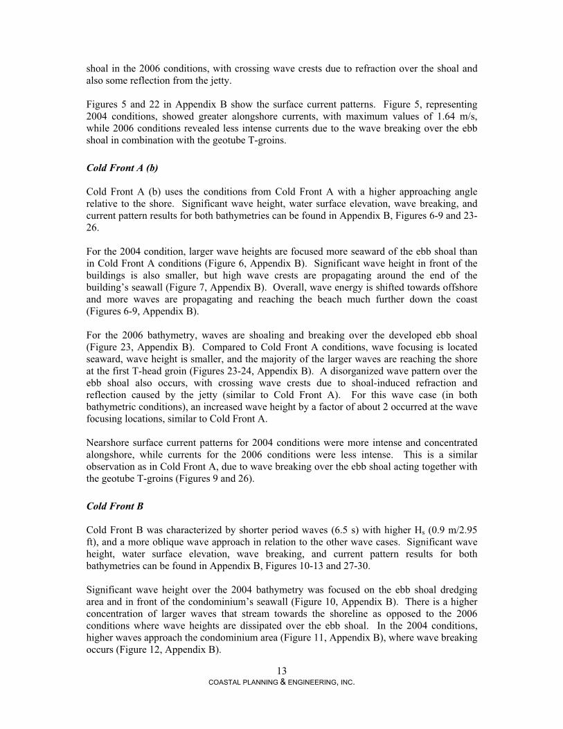
Model Validation Comments and Conclusions After running BOUSS-2D with the selected wave cases, it was observed that the model was able to simulate the observed wave breaking conditions with reliable accuracy. Figure 13 below provides an example of model results compared to a photograph, showing that it approximates the general wave propagation and breaking conditions for this region. The upper panel shows an October 2003 aerial photo provided by the Pinellas County staff which represents the pre-2004 conditions. The picture shows waves approaching obliquely from the northwest with bending due to refraction in shallow waters in front of the northern seawalls. This situation occurred in simulations of Cold Fronts A, A(b) and B, shown in the 3 lower


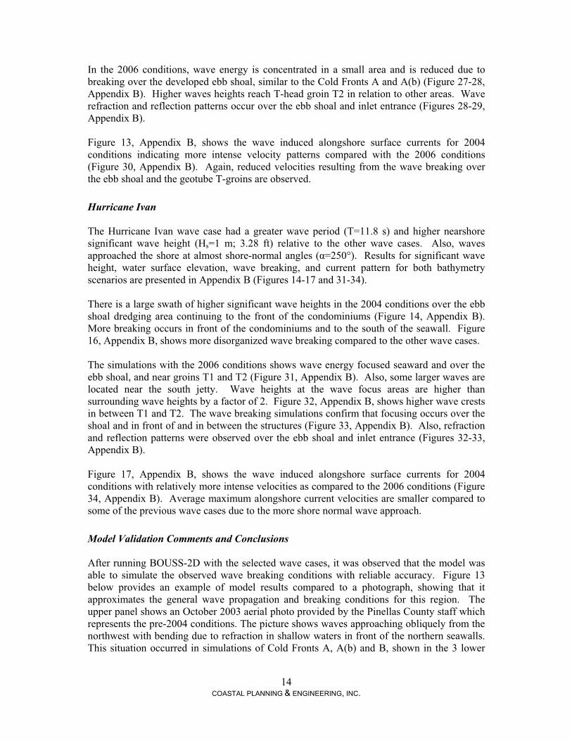
panels of Figure 13. A view from the beach from the simulation of Cold Front A(b) is provided in Figure 14 for additional perspective.

Figure 13. Model validation in relation to wave characteristics and peel angle. Red

arrows represent wave directions and red circles identify the breaking waves.

Figure 14. Model result for 2004 condition with Cold Front A (b), showing wave

refraction and breaking around the front of the condominium’s seawall.


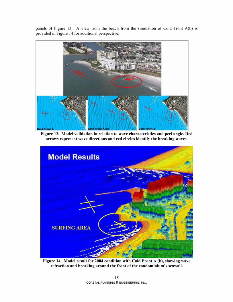
In addition to good agreement between modeled wave breaking patterns and observations, the wave cases selected for the production runs were compared to online documentation of good surfing days at Upham Beach (Cold Fronts A, A(b), B, and Hurricane Ivan). Figure 15 shows pictures taken at Upham Beach at the two simulated cold fronts (Source: www.wannasurf.com). The left panel photo was taken on 12/09/2003 and the right panel on 12/17/2003 (note the condominium fence). Both days represented favorable wave size and peel angle for surfing. The wave peel angle is an important surfability parameter that can be estimated as the angle � between the wave crest and the breaker line (Walker, 1974).

Figure 15. Surfing condition in front of condominium at the modeled Cold Front A and

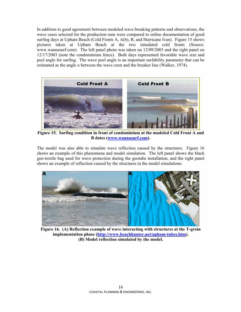
B dates (www.wannasurf.com). The model was also able to simulate wave reflection caused by the structures. Figure 16 shows an example of this phenomena and model simulation. The left panel shows the black geo-textile bag used for wave protection during the geotube installation, and the right panel shows an example of reflection caused by the structures in the model simulations.

Figure 16. (A) Reflection example of wave interacting with structures at the T-groin

implementation phase (http://www.beachhunter.net/upham-tubes.htm). (B) Model reflection simulated by the model.


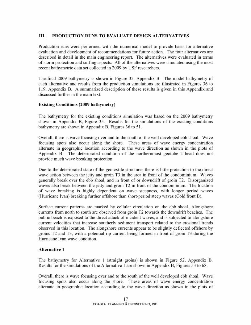
III. PRODUCTION RUNS TO EVALUATE DESIGN ALTERNATIVES Production runs were performed with the numerical model to provide basis for alternative evaluation and development of recommendations for future action. The four alternatives are described in detail in the main engineering report. The alternatives were evaluated in terms of storm protection and surfing aspects. All of the alternatives were simulated using the most recent bathymetric data set collected in 2009 by USF researchers. The final 2009 bathymetry is shown in Figure 35, Appendix B. The model bathymetry of each alternative and results from the production simulations are illustrated in Figures 36 to 119, Appendix B. A summarized description of these results is given in this Appendix and discussed further in the main text.

Existing Conditions (2009 bathymetry) The bathymetry for the existing conditions simulation was based on the 2009 bathymetry shown in Appendix B, Figure 35. Results for the simulations of the existing conditions bathymetry are shown in Appendix B, Figures 36 to 51. Overall, there is wave focusing over and to the south of the well developed ebb shoal. Wave focusing spots also occur along the shore. These areas of wave energy concentration alternate in geographic location according to the wave direction as shown in the plots of Appendix B. The deteriorated condition of the northernmost geotube T-head does not provide much wave breaking protection. Due to the deteriorated state of the geotextile structures there is little protection to the direct wave action between the jetty and groin T3 in the area in front of the condominium. Waves generally break over the ebb shoal, and in front of or downdrift of groin T2. Disorganized waves also break between the jetty and groin T2 in front of the condominium. The location of wave breaking is highly dependent on wave steepness, with longer period waves (Hurricane Ivan) breaking further offshore than short-period steep waves (Cold front B). Surface current patterns are marked by cellular circulation on the ebb shoal. Alongshore currents from north to south are observed from groin T2 towards the downdrift beaches. The public beach is exposed to the direct attack of incident waves, and is subjected to alongshore current velocities that increase southerly sediment transport related to the erosional trends observed in this location. The alongshore currents appear to be slightly deflected offshore by groins T2 and T3, with a potential rip current being formed in front of groin T3 during the Hurricane Ivan wave condition.

Alternative 1 The bathymetry for Alternative 1 (straight groins) is shown in Figure 52, Appendix B. Results for the simulations of the Alternative 1 are shown in Appendix B, Figures 53 to 68. Overall, there is wave focusing over and to the south of the well developed ebb shoal. Wave focusing spots also occur along the shore. These areas of wave energy concentration alternate in geographic location according to the wave direction as shown in the plots of


Appendix B. Due to the absence of heads on the straight groins, there is little protection to the direct wave action in the cells between successive structures. Waves generally break on the ebb shoal and near the structures. Depending on the wave steepness, the waves break in front of the straight groins and wrap around the groin’s tips, near the groin tips or between groin compartments. Waves seem to peel adjacent to the straight groins providing a condition favorable to surfing. However, the lack of T-heads means less wave protection for the beaches in between groins and potential for rip current generation as evidenced in the current plots in Appendix B. Surface current patterns are marked by large cellular circulation on the ebb shoal, alongshore currents interrupted by the groins, and small cellular circulations between structures. Small rip currents are observed between groin compartments against the southernmost groin of each cell. A more persistent rip-current is observed in front of the public beach on the north side of groin T3. This alternative has a potential of being surfer-friendly, but has reduced potential for storm-protection due to the absence of a T-head section that acts as a breakwater on the groins.

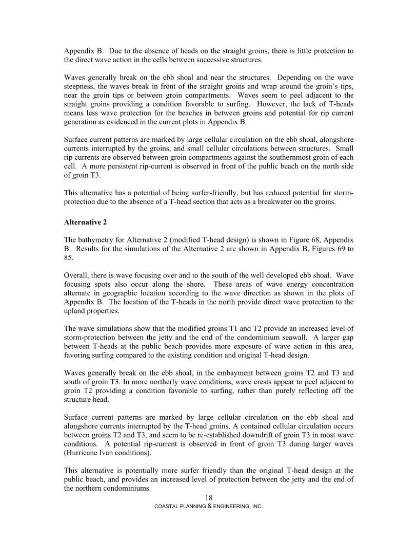
Alternative 2 The bathymetry for Alternative 2 (modified T-head design) is shown in Figure 68, Appendix B. Results for the simulations of the Alternative 2 are shown in Appendix B, Figures 69 to 85. Overall, there is wave focusing over and to the south of the well developed ebb shoal. Wave focusing spots also occur along the shore. These areas of wave energy concentration alternate in geographic location according to the wave direction as shown in the plots of Appendix B. The location of the T-heads in the north provide direct wave protection to the upland properties. The wave simulations show that the modified groins T1 and T2 provide an increased level of storm-protection between the jetty and the end of the condominium seawall. A larger gap between T-heads at the public beach provides more exposure of wave action in this area, favoring surfing compared to the existing condition and original T-head design. Waves generally break on the ebb shoal, in the embayment between groins T2 and T3 and south of groin T3. In more northerly wave conditions, wave crests appear to peel adjacent to groin T2 providing a condition favorable to surfing, rather than purely reflecting off the structure head. Surface current patterns are marked by large cellular circulation on the ebb shoal and alongshore currents interrupted by the T-head groins. A contained cellular circulation occurs between groins T2 and T3, and seem to be re-established downdrift of groin T3 in most wave conditions. A potential rip-current is observed in front of groin T3 during larger waves (Hurricane Ivan conditions). This alternative is potentially more surfer friendly than the original T-head design at the public beach, and provides an increased level of protection between the jetty and the end of the northern condominiums.


Alternative 3 The bathymetry for Alternative 3 (curved T-head design) is shown in Figure 86, Appendix B. Results for the simulations of the Alternative 3 are shown in Appendix B, Figures 87 to 102. A surfing reef is included in Alternative 3 and has a submerged crest at 1.22 m (4 ft) water depth MSL (Figure 17). The crest of the reef has a constant width of approximately 1m (3.28 ft) to promote breaking during smaller wave conditions. The seaward slope is approximately of 1V:22.5H.

Figure 17. Artificial reef of Alternative 3, lateral view.

Overall, there is wave focusing over and to the south of the well developed ebb shoal. However, in this alternative, another zone of wave focusing is observed due to wave breaking over the submerged artificial reef. Wave focusing spots also occur along the shore. These areas of wave energy concentration change location according to the wave direction as shown in the plots of Appendix B. Landward of the surfing reef, reduced wave heights are observed closer to the beach (i.e., a wave shadowing effect). Wave breaking occurs at the well developed offshore ebb shoal and also over the surfing reef. Nearshore breaks are disorganized directly landward of the reef (straight groin area, but exhibits regular patterns south of groin T3. Wave peeling over the reef provides an open wave face favorable for surfing in the moderate wave conditions tested here. Smaller waves may pass over the reef without breaking. Surface current patterns are dominated by one large cellular circulation over the ebb shoal and one or two smaller circulation cells near the surfing reef, depending on the wave conditions. Alongshore currents are weakened by the offshore surfing reef and T-groins, and are re-established after the last T-head groin to the south. The reduced currents near the


beach leeward of the reef represent a multi-purpose benefit of providing coastal protection and recreation. The wave simulations show that modified groins T1 and T2 provide a level of storm-protection similar to the existing design in the area between the jetty and the end of the condominium seawall. Because of the surfing reef, increased protection and favorable surfing conditions are provided in front of the public beach. This alternative provides the most benefit to the surfing community compared to the other design alternatives tested due to the presence of the surfing reef. However, it provides less storm-protection than Alternative 2 in the heavily eroded area between the jetty and the end of the condominium. Lastly, this is likely the most expensive of all the alternatives due to the costs associated with installing the surfing reef.

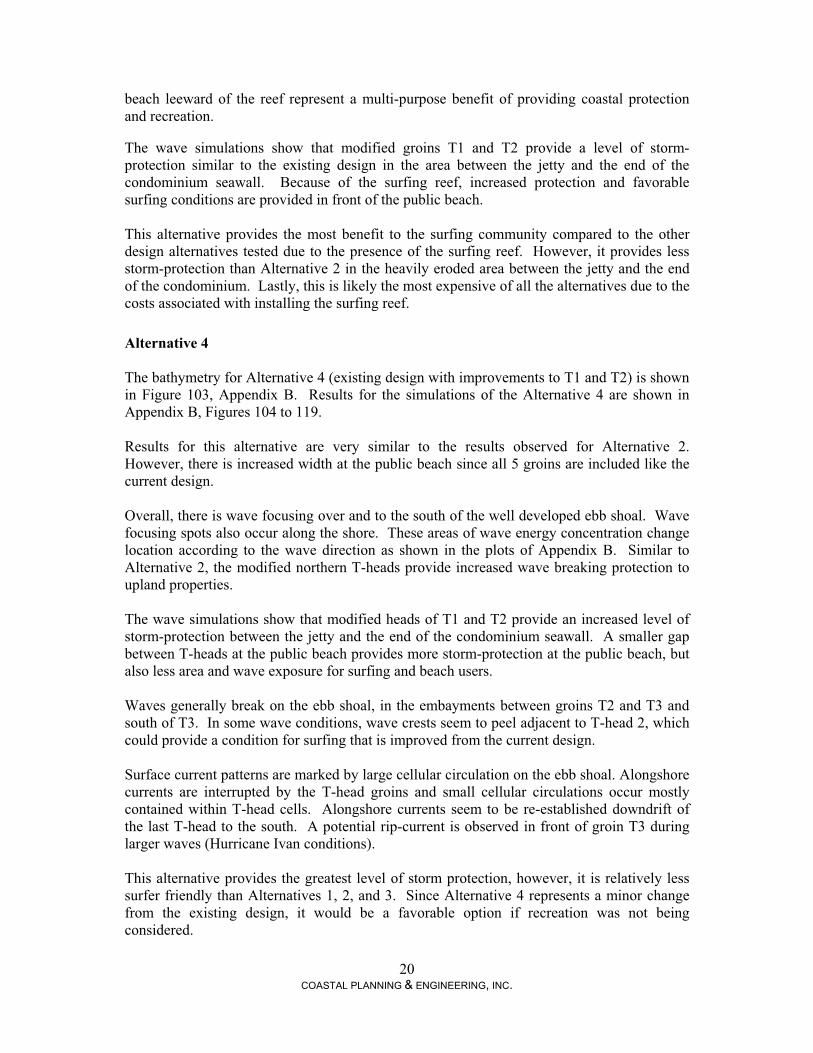
Alternative 4 The bathymetry for Alternative 4 (existing design with improvements to T1 and T2) is shown in Figure 103, Appendix B. Results for the simulations of the Alternative 4 are shown in Appendix B, Figures 104 to 119. Results for this alternative are very similar to the results observed for Alternative 2. However, there is increased width at the public beach since all 5 groins are included like the current design. Overall, there is wave focusing over and to the south of the well developed ebb shoal. Wave focusing spots also occur along the shore. These areas of wave energy concentration change location according to the wave direction as shown in the plots of Appendix B. Similar to Alternative 2, the modified northern T-heads provide increased wave breaking protection to upland properties. The wave simulations show that modified heads of T1 and T2 provide an increased level of storm-protection between the jetty and the end of the condominium seawall. A smaller gap between T-heads at the public beach provides more storm-protection at the public beach, but also less area and wave exposure for surfing and beach users. Waves generally break on the ebb shoal, in the embayments between groins T2 and T3 and south of T3. In some wave conditions, wave crests seem to peel adjacent to T-head 2, which could provide a condition for surfing that is improved from the current design. Surface current patterns are marked by large cellular circulation on the ebb shoal. Alongshore currents are interrupted by the T-head groins and small cellular circulations occur mostly contained within T-head cells. Alongshore currents seem to be re-established downdrift of the last T-head to the south. A potential rip-current is observed in front of groin T3 during larger waves (Hurricane Ivan conditions). This alternative provides the greatest level of storm protection, however, it is relatively less surfer friendly than Alternatives 1, 2, and 3. Since Alternative 4 represents a minor change from the existing design, it would be a favorable option if recreation was not being considered.


IV. CONCLUSIONS A numerical model study of wave transformation, breaking and wave-induced currents was conducted to evaluate the performance of a series of structural alternatives developed for Upham Beach. The alternatives were evaluated for a series of wave events in terms of storm protection and surfing/recreation as described below:

1. Storm Protection and Erosion Control: Alternative 4, which resembles the current design with some storm-protection improvements, is the alternative that provides the greatest level of storm protection. Alternative 2 has a similar level of protection for the upland properties. This is followed by Alternative 3 and 1 in order from higher to lower level of storm protection.

2. Surfing Friendly Factor: Alternative 3 is the most surfer-friendly alternative due to

the introduction of the surfing reef design component. Alternative 1 also has benefits for surfing due to the straight groins. Alternative 2 would not totally address surfing concerns, but would provide an area for surfers and other recreational beach users. Alternative 4 would have similar effects as the current design.

Alternative 2 is the recommended approach since it provides an increased level of storm-protection at the critically eroded area and more open space for surfing and recreation when compared to the original T-head design and Alternative 4. Alternative 1 is not recommended due to the potential for a reduced level of storm protection and possible rip current generation at the public beach. Alternative 3 provides a reasonable level of storm protection (similar to the original design) and improvement to surf resources, but the most costly alternative. The artificial reef could be combined with any alternative to provide a surfing amenity and additional coastal protection. The final alternative selection should consider stakeholder input, storm protection, impact to recreational uses of the beach, costs and potential permitting restrictions.

V. REFERENCES Benedet. L.; Finkl, C.W.; Klein, A.H.F. (2004) Classification of Florida Atlantic Beaches: Sediment variation, morphodynamics and coastal hazards. Journal of Coast Research, SI 39. Coastal Planning & Engineering, Inc. 1992. Blind Pass Inlet Management Plan. Boca Raton, FL: Coastal Planning & Engineering, Inc., 69 pp. Davis, R. A., Jr., 1989. “Management of drumstick barrier islands”. Proc. of the 6th Symposium on Coastal and Ocean Man., Charleston, SC, ASCE, 16 pp. Elko, N.; Mann, D. W., 2007. Implementation of Geotextile T-Groins in Pinellas County, Florida. Shore & Beach, Vol. 75, No. 2. Spring 2007. 9 pp. Hutt, J.A.; Black, K.P.; Mead, S.T. (2001). Classification of surf breaks in relation to surfing skill. Journal of Coast Research.. SI 29. 66-81 p. NOAA Coastal Services Center. Digital Coast: Data Access Viewer. 2009. http://www.csc.noaa.gov/ldart.


Nwogu, O.G.; Demirbilek, Z., 2001. BOUSS-2D: A Boussinesq Wave model for coastal regions and harbors. USACE Coastal and Hydraulics Laboratory Technical Report A492004. 92 p. Silvester and Hsu (1993) Coastal Stabilization. World Scientific.578 p. Walker, J.R. (1974). Recreational Surf Parameters. Technical report 30, Look Laboratory, University of Hawaii. 311 p. WannaSurf.com, Miscellaneous photos, http://www.wannasurf.com

COASTAL PLANNING & ENGINEERING, INC.

VI. APPENDIX A-1 Hm0: This is used as an estimate of significant wave height (Hs) and is the most commonly referenced, Hm0 = 4*sqrt (sum(S)), where S (f) is the energy distribution. Tp: Peak Period, this is the period associated with the frequency that has the most energy (or peak). It is defined as Tp = 1/f (max(S(f)). DirTp: Peak direction is the direction at the peak frequency. SprTp: Peak Spreading is a measure of how much variance there is with the directional estimates. High values may be thought of as a poorly organized wave field whereas low values suggest waves coming from more or less the same direction.

APPENDIX A MODELING REPORT - Pinellas County, …...COASTAL PLANNING & ENGINEERING, INC. UPHAM BEACH...

Documents

Transcript of APPENDIX A MODELING REPORT - Pinellas County, …...COASTAL PLANNING & ENGINEERING, INC. UPHAM BEACH...