APPENDIX A. Determination of the Bootstrap Confidence ... · APPENDIX A. Determination of the...

APPENDIX A. Determination of the Bootstrap Confidence Interval Quantiles The definition of a confidence interval for coefficient θ is

(A.1) , ( )Pr L U Pθ θ θ≤ ≤ ≥ c

)

⎤⎥

where is the coverage probability (for example, for a 90-percent confidence interval, equals 0.9), and

and are the lower and upper bounds on the confidence interval. Specific values for and are obtained

by imposing the additional constraint that the confidence interval is to have equal probability in the tails such that

cP cP Lθ

Uθ Lθ Uθ

(A.2) , ( ) (Pr PrL Uθ θ θ θ> = <

to the extent possible, given the constraint in equation (A.1).

Let there be R bootstrap replications, ordered in ascending order. We seek the ranks of the R replications that serve as the lower and upper bounds and defined above. To satisfy equation (A.1), the number of

replications within the bounds, including the replications that define the bounds, must equal , where

Lθ Uθ

cP R⎡⎢ ⎡ ⎤⎢ ⎥

defines the ceiling function corresponding to the next highest integer for its argument. Consequently, there are

( )1c cR P R P R⎢⎡ ⎤− = −⎢ ⎥ ⎣ ⎥⎦ replications excluded from the interval, where ⎢ ⎥⎣ ⎦ is the floor function corresponding

to the next lowest integer for its argument. In order to satisfy equation (A.2), the number of excluded replications at the bottom must match, as closely as possible, the number of excluded replications at the top. We

take the number of excluded replications from the bottom to be one-half of ( )1 cP R− rounded to the next

lowest integer. Therefore the lower bound of the confidence interval is determined by the ( )1 2cR P⎢ ⎥− +⎣ ⎦ 1

ordered bootstrap replication. In order to satisfy equation (A.1), this implies there are

( )1cR P R R P⎢⎡ ⎤− − −⎢ ⎥ ⎣ 2c⎥⎦ replications excluded from the top. The rank determining the upper bound is given

by R minus the number of replications excluded from the top, which is ( )1 2c cP R R P⎢ ⎥⎡ ⎤ + −⎢ ⎥ ⎣ ⎦ .

The SPARROW Surface Water-Quality Model: Theory, Application and User Documentation

204

APPENDIX B. Hydrologic Network Development Each reach in the SAS input data file for the SPARROW model must be assigned a unique numerical

sequence code indicating downstream ordering from headwater to terminal reaches. The preprocessing steps described here can be used to assign the hydrologic sequence code based on node topology of the digital stream network. Note that these pre-processing steps were previously completed for the national Reach File 1 (RF1) network data set (Nolan and others, 2002); the corresponding SAS reach data set used for calibration and prediction (“sparrow_data1”) already contains the variables produced in step 3 below.

In the following discussion, ‘[…]’ represents the path on the user’s computer containing the sparrow software package.

1. Create a flat file (reach.dat) from the arc attribute table (aat) associated with the reach coverage**: [**The package for the example model application does not include the reach coverage (rather, it contains only the .e00 export file) due to size considerations, and therefore it is not possible to run this first step for the example. The description of this first step is included here to guide the user in preparing a file for preprocessing.] Using a text editor, edit the file “extract_reachaat.aml” (in “[…]\sparrow\master\preprocess”) to conform to the directory structure, name of the reach coverage, and names of various coverage attributes for this application (program listing shown in table B1). Specific instructions for editing are included as comments within the AML file. Run the AML in the Arc environment, using the command “&r d:\sparrow\master\preprocess\extract_reachaat.aml”; the output file reach.dat is written to the directory “[…]\sparrow\data.”

2. Calculate the hydrologic sequence code and total upstream drainage area for each reach: Copy the FORTRAN program “assign_hydseq.exe” (in “[…]\sparrow\master\preprocess,” documentation shown in table B2) to the directory “[…]\sparrow\data.” Execute the program from the data directory [note: if the default settings for the national RF1 coverage were used in the AML in step 1, then answer ‘Yes’ to the first question and ‘No’ to the second question]. Examine the output files “hydseq.dat,” “nohydseq.dat,” and “tarea.dat” to validate connectivity of the stream network information in the reach coverage and to compare accumulated drainage areas (calculated by “assign_hydseq.exe”) to known drainage areas at certain locations. (See description of these files in table B2, “Documentation for the preprocessing program ‘assign_hydseq.exe.’”)

3. Merge the hydrologic sequence code and total upstream drainage area for each reach to the ASA input data file “sparrow_data1”: Edit the SAS program “merge_hydseq.sas” (program listing shown in table B3) to conform to the directory structure for this application. Run the program to overwrite the existing “sparrow_data1” dataset with a new version containing the variables hydseq (column label “HYDROLOGIC SEQUENCE NUMBER”) and demtarea (column label “TOTAL DRAINAGE AREA”).

Appendix B. Hydrologic Network Development 205

Table B1. Listing of the preprocessing program “extract_reachaat.aml.”

/*---------------------------------------------------------------------- /* /* Command name: EXTRACT_REACHAAT.AML /* Language: AML /* /*:::::::::::::::::::::::::::::::::::::::::::::::::::::::::::::::::::::: /* /* Purpose: Extracts necessary attributes from the /* arc attribute table (aat) of the ArcInfo reach coverage /* for input to assign_hydseq FORTRAN program /* /*:::::::::::::::::::::::::::::::::::::::::::::::::::::::::::::::::::::: /* /* Comments: /* /* History: /* Author/Site, Date, Event /* ------------------------------------------------------------ /* R. Alexander 09/10/03 Created /*:::::::::::::::::::::::::::::::::::::::::::::::::::::::::::::::::::::: /* Edit the pathname for the directory containing the ArcInfo reach coverage as /* necessary &workspace D:\sparrow\data &DATA arc info ARC CALC $NM = 1 CALC $COMMA-SWITCH = -1 CALC $PRINTER-SIZE = 200 /* Edit the name of the aat as necessary SEL ERF1_2_L.AAT /* Edit the name of the attribute for the unique reach identifier /* as necessary SORT E2RF1 RESEL E2RF1 LT 80000 /************************************ /* Output reach attributes for non-coastal reaches /* Edit the path for the output file as necessary, but retain the /* name reach.dat for the output file. /* Edit attribute names as necessary. /************************************ OUTPUT D:\sparrow\data\reach.dat INIT PRINT E2RF1,FNODE#,TNODE#,DEMIAREA,FRAC,HUC2 ASEL/* Edit the aat file name as necessary (retain the # symbol) SORT ERF1_2_L# Q STOP &END &RETURN


206

Table B2. Documentation for the preprocessing program “assign_hydseq.exe.”

Program “assign_hydseq.exe” Programmed by R.B. Alexander December 20, 2002 Revised: January 28, 2003

PURPOSE: The program creates the attribute variables HYDSEQ and DEMTAREA, which are output to two separate data files, for use in version 2.0

of the SPARROW model.

The output file HYDSEQ.DAT contains hydrologically ordered (from upstream to downstream) river reach records for use in computing total drainage areas and summing constituent mass in the SPARROW model.

The output file TAREA.DAT contains values of the total drainage area (DEMTAREA) for the watershed above the outlet of each river reach.

The optional output file REACHSTA.DAT contains the monitoring station ID of the nearest downstream monitoring station—can be used to identify reaches with monitoring sites (for comparison of total drainage areas calculated using this program with other estimates of drainage area).

DATA REQUIREMENTS: The river reach file must be topologically correct (full connectivity) and contain a from-node (FNODE) and to-node (TNODE) number for

every reach in the domain. Flow direction is FROM-TO. The maximum limits of the program are 600,000 reach segments. The program can handle up to a maximum of four tributary reaches converging on a single reach node and can handle a maximum of two diverging reaches. The values of reach and to- and from-node numbers (WATERID, FNODE, and TNODE) must not exceed 600,000.

In computing the total reach drainage area, the fractional diversion (FRAC) assumes braided channels for values less than 1.0 (i.e., the total drainage area of the upstream reach is multiplied by FRAC in computing the total area of the downstream reach).

The user may select to have the program identify headwater reaches. Headwater reaches (HEADFLAG=1) are identified as those reaches where the FROM node has no matching TO node.

FILE STRUCTURE AND CONTENTS:

INPUT FILE (REACH.DAT; free-format with each variable separated by a blank) WATERID - unique identification number for the reach FNODE - reach from-node (upstream node) TNODE - reach to-node (downstream node) DEMIAREA - incremental drainage area of the reach catchment FRAC - Water diversion fraction indicating the fractional share of the water received from the upstream reach STAID - Unique monitoring station identification number associated with the reach (set to zero if the reach contains no monitoring

station) HEADFLAG - optional headwater reach flag (0=non-headwater reach; 1=headwater reach)—A value should NOT be included in the

file if the user wants the program to automatically identify headwater reaches

OUTPUT FILE (HYDSEQ.DAT) HYDSEQ - Hydrologic sequence code indicating the downstream order of the river reach WATERID - unique identification number for the reach FNODE - reach from-node (upstream node) TNODE - reach to-node (downstream node) DEMIAREA - incremental drainage area of the reach catchment FRAC - Water diversion fraction indicating the fractional share of the water received from the upstream reach (1=no diversion) HEADFLAG - headwater reach flag (0=non-headwater reach; 1=headwater reach)

OUTPUT FILE (NOHYDSEQ.DAT) WATERID - unique identification number for reaches not assigned a HYDSEQ number. These may reflect non-connected or

improperly flipped reaches.

OUTPUT FILE (TAREA.DAT) WATERID - unique identification number for the reach DEMTAREA - total drainage area of the watershed upstream from the reach outlet

OPTIONAL OUTPUT FILE (REACHSTA.DAT) WATERID - unique identification number for the reach STAID - Unique monitoring station identification number of the nearest downstream station

Appendix B. Hydrologic Network Development 207

Table B3. Listing of the preprocessing program “merge_hydseq.sas”

/* Program: merge_hydseq.sas Function: Combines DATA1 (containing all required variables for reaches incremental watersheds except for HYDSEQ and DEMTAREA) with output from the assign_hydseq FORTRAN program. Creates illustration dataset for SPARROW version 2.1 Created : R. Alexander Date : 09/10/03 */ LIBNAME DIR 'D:\sparrow\data' ; FILENAME HYDSEQ 'D:\sparrow\data\hydseq.dat'; FILENAME TAREA 'D:\sparrow\data\tarea.dat'; /* input hydrologic sequence number */ DATA HYDSEQ; INFILE HYDSEQ ; INPUT HYDSEQ WATERID FNODE TNODE DEMIAREA FRAC HEADFLAG; KEEP WATERID HYDSEQ; RUN; /* input total accumulated drainage area */ DATA TAREA; INFILE TAREA ; INPUT WATERID DEMTAREA; RUN; PROC SORT DATA=HYDSEQ; BY WATERID; PROC SORT DATA=TAREA; BY WATERID; PROC SORT DATA=DIR.SPARROW_DATA1; BY WATERID; RUN; /* merge input data with existing SAS DATA1 file */ DATA DIR.SPARROW_DATA1; MERGE HYDSEQ TAREA DIR.SPARROW_DATA1; BY

WATERID; LABEL HYDSEQ = 'HYDROLOGIC ORDERING NUMBER' DEMTAREA = 'TOTAL DRAINAGE AREA (KM2)' ;

RUN;


208

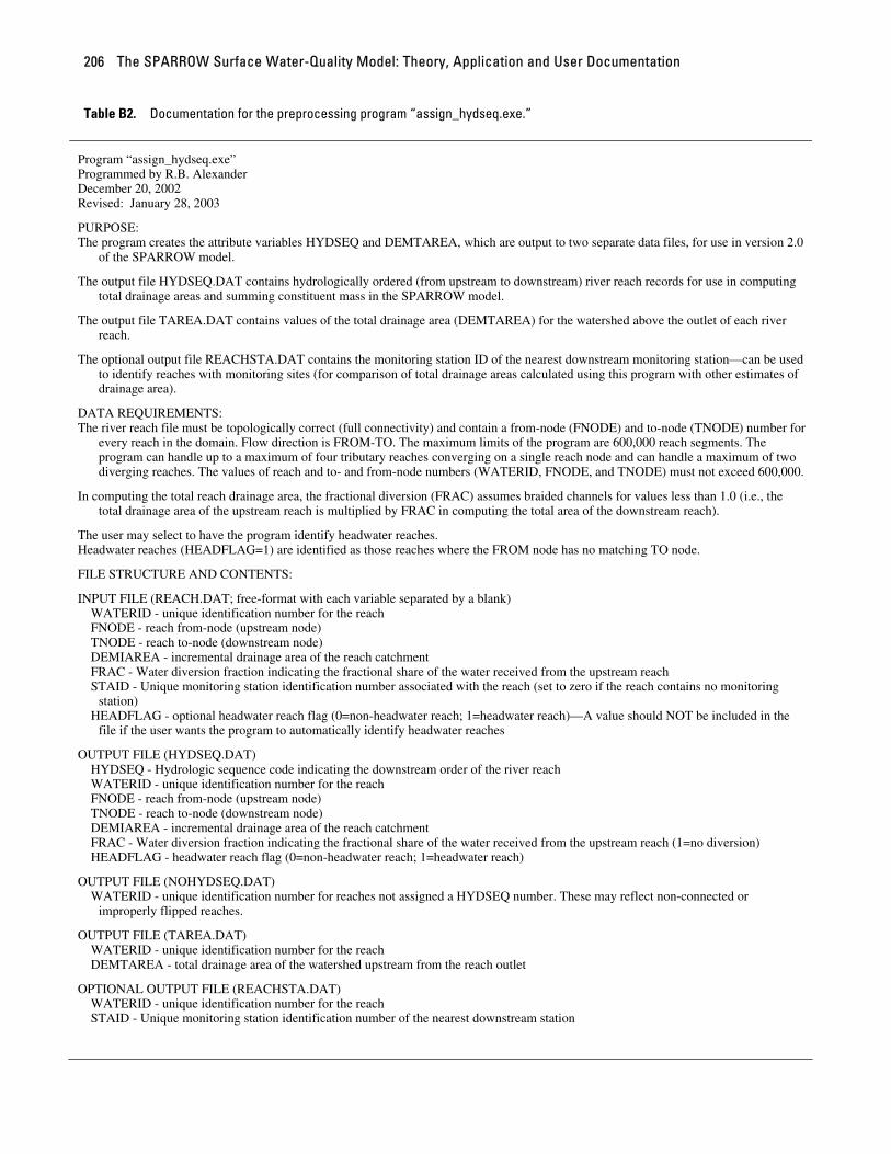
APPENDIX C. SAS/GIS Mapfile Creation The SAS program “sparrow_create_gis.sas” creates SAS/GIS datasets (mapfiles and layers) from the

ArcInfo coverages supplied by the user. The SAS/GIS mapfiles and layers are then used in combination with SPARROW model output to produce maps of calibration residuals and reach predictions after each model run. Certain SAS/GIS features can not be specified, however, in the execution of “sparrow_create_gis.sas”; these include break points for intervals for thematic variables and various map display properties such as projection format, legend, and color. These processing steps must be done manually by the user after running “sparrow_create_gis.sas,” working with the mapfiles in the SAS/GIS user interface. The user need make these changes only once; the user then saves the altered version of the mapfiles and re-uses them with all successive model runs. It is recommended that these changes be made immediately after running “sparrow_create_gis.sas.”

The SPARROW package downloaded from the SPARROW software web page contains files that can serve as a visual aid in the following discussion.

I. Create the SAS/GIS layers and mapfiles using “sparrow_create_gis.sas”

The ArcInfo coverages (in noncompressed, export file format) of the reach network and state-boundaries base map (files named “erf1_2_l.e00” and “states2mprjp.e00,” respectively, in the zip file “sparrow_gis_exports.zip”) must be converted to SAS/GIS spatial data sets so that SAS can produce thematic maps of model output as part of each model run (see section 2.8.4, “GIS maps”).

First, edit the header information in the SAS program “sparrow_create_gis.sas” (in the directory “[…]\sparrow\master\preprocess”) so that path names for the \gis and \results directories, and path and file names for the Arc export (.e00) files correspond with the directory structure described in section 2.3, “Obtaining and installing software.” Then run the “sparrow_create_gis.sas” program to convert the Arc export files to SAS/GIS data sets. Execution of this program may take several minutes, due to the size of the reach coverage for the demonstration model.

This first step may be omitted for the purpose of the demonstration model, and the user may execute the remainder of the steps using the SAS/GIS layers and mapfiles provided in the main SPARROW package zip file. Note that the program “sparrow_create_gis.sas” can be run in two different modes (as specified by the “if_previous” switch); the create mode (as currently specified) or the update mode. In create mode, the program imports the Arc export files and saves the information as SAS/GIS mapfiles and layers. In update mode, the program simply updates existing mapfiles and layers with specified model output files. The update mode is useful when a user wants to view maps of results from an earlier (other than the most recent) model run, but doesn’t wish to rerun the SPARROW program (which automatically updates the mapfiles and layers by re-linking them to the most recent model output files).

II. Specify additional SAS/GIS features for the SAS/GIS layers and mapfiles

The SAS/GIS mapfiles (“resids”, “resids_map”, and “reach_map”) and layers are edited manually to specify the thematic and display properties for the maps of model output. The detailed instructions for the manual edits that follow also are included as comments within the “sparrow_create_gis.sas” program. The user need make these changes to the mapfiles and layers only once.

A. Modify the mapfile “resids” to specify theme intervals and symbols for the layer “Mapresids”

1. Load the mapfile “resids” into SAS/GIS. In the top level of the SAS Explorer window, double-click Libraries, the library “Dir_gis,” the catalog “Resids,” and the globe-shaped icon for the GIS mapfile “Resids.” If the user is editing the mapfiles at the beginning of a new SAS session (separate from running sparrow_create_gis.sas), the user must specify the directories (by assigning them SAS library names) that contain the SAS/GIS data sets and the SPARROW model output files. See section 2.5.4, “Opening SAS data files from the SAS Explorer window,” for instructions on assignment of a SAS library.

Appendix C. SAS/GIS Mapfile Creation 209

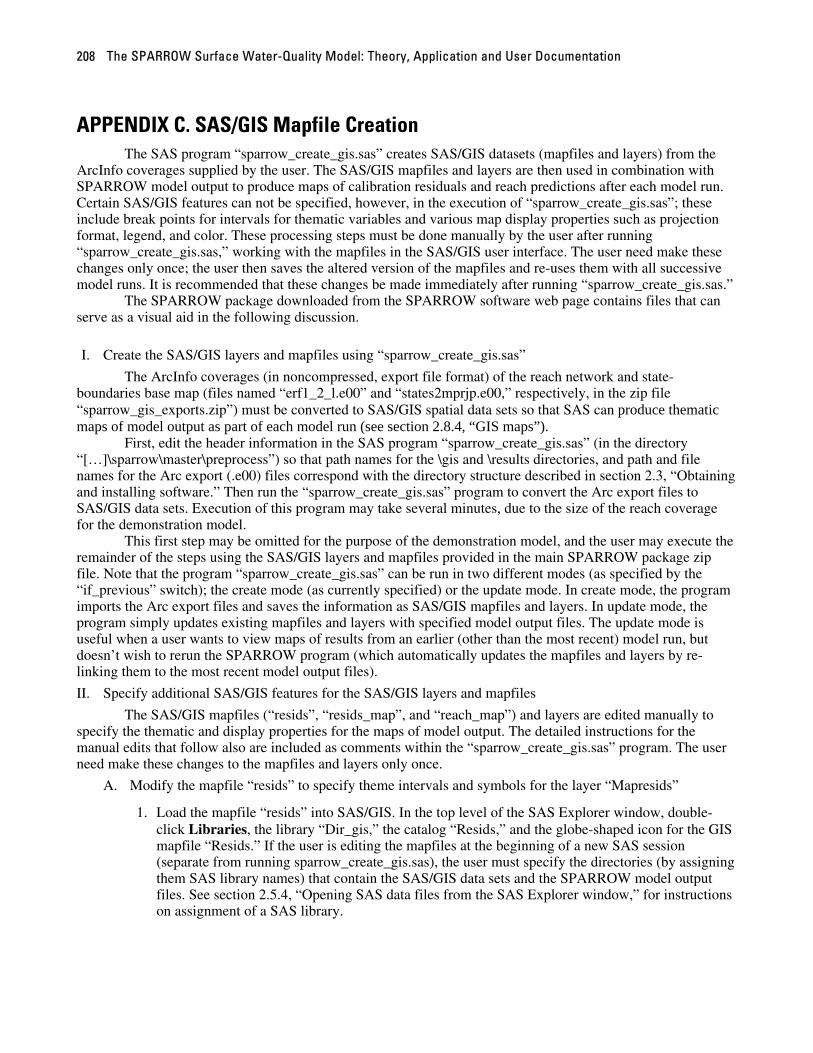
2. The GIS Map window should display the layer “Mapresids” as indicated by the layer button MAPRESIDS at the top of the map window. “Mapresids” is a SAS/GIS point layer containing information for the monitoring stations. If the SPARROW model had not been executed prior to when this maplayer was created by the “sparrow_create_gis.sas” program (so that the output data file named “resids” had not been generated in the “[…]\sparrow\results” directory), the set of points and attributes in the “Mapresids” layer are temporary until the model is executed (providing structure for the linkage between the layer and the expected model output file of calibration residuals). In such cases the layer contains 10 randomly generated point locations; otherwise, it contains the stations from the latest model run.


210

3. Right-click the MAPRESIDS layer button and select Edit. In the GIS Layer window, verify that the Thematic button is switched on. If the SAS program “sparrow_create_gis.sas” ran smoothly, it established a thematic link between the layer “Mapresids” and the model output data file “Resids” in the SAS library “dir_rslt,” and also specified which variable from the data file “Resids” is to be used as the map theme (the variable map_resid, which is the studentized residual calculated for each monitoring station during model estimation). The link between “Mapresids” and “Resids” can be established even without a pre-existing SPARROW model run and output file, because in this case the program “sparrow_create_gis.sas” creates an empty shell of the file “Resids” and saves it to a directory with SAS library name “dir_rslt.”

4. Specify the theme intervals for the layer “Mapresids.” Click the Theme Range box to open the GIS Thematic Layer Ranges window; click Specified and specify interval break points 1.5, 0, and -1.5 as follows:

a. Click Add Break, enter the value -1.5, and click Apply.

b. Click Add Break, enter the value 1.5 and click Apply.

c. Click Remove Break, select all values except -1.5, 0, and 1.5, and click Apply.

d. Click OK to return to the GIS Layer window.


5. To modify colors and sizes of the theme symbols from the default selections displayed in the boxes, click each box and specify the selection.

6. Close the Layer window (click the X button in the top right corner).

7. Save the changes to the mapfile “resids” by selecting File, Save, All from the menu bar.

B. Modify map display properties for the mapfile “resids_map”

1. Load the mapfile “resids_map” into SAS/GIS. To do this, click on the SAS Explorer window and return to the “Dir_gis” library level. Double-click the catalog “Resids_map,” then the globe-shaped icon for the GIS mapfile “Resids_map.”

2. The GIS Map window should display two layers, “States2m” (the layer created from the Arc export file of state boundaries in the example application) and “Mapresids”; if this is not the case, make sure that the buttons STATES2M and MAPRESIDS at the top of the map window are switched to on. The boundaries for states should be displayed as detailed boundaries: if this is not the case, right click the STATES2M layer button and select Show Details.

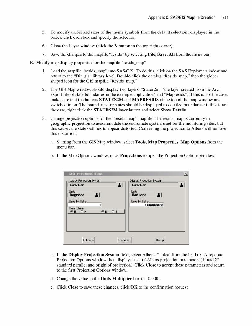
3. Change projection options for the “resids_map” mapfile. The resids_map is currently in geographic projection to accommodate the coordinate system used for the monitoring sites, but this causes the state outlines to appear distorted. Converting the projection to Albers will remove this distortion.

a. Starting from the GIS Map window, select Tools, Map Properties, Map Options from the menu bar.

b. In the Map Options window, click Projections to open the Projection Options window.

c. In the Display Projection System field, select Alber's Conical from the list box. A separate Projection Options window then displays a set of Albers projection parameters (1st and 2nd standard parallel and origin of projection). Click Close to accept these parameters and return to the first Projection Options window.

d. Change the value in the Units Multiplier box to 10,000.

e. Click Close to save these changes, click OK to the confirmation request.


212

4. Enable the mapfile to display, in an FSView table, values from the layer “Mapresids” and the attribute dataset “Resids” for any selected (clicked) point on the map:

a. Starting from the GIS Map window, select Actions, Define from the menu bar.

b. In the Action Definitions window, click the scroll arrow for the Type box and select VIEW.

c. The field Data Link will appear below the Type field, with MAPRESIDS displayed in the list box. MAPRESIDS is the link (created and named during the execution of the “sparrow_create_gis.sas”) between the attribute data file “Resids” and the layer “Mapresids.” Examine the link definition by clicking the right-arrow button on the Data Link box: the Attribute Data Sets window displays variables from the data file “Resids” in the Data Set Vars box and variables from the spatial data set in the Composites box. This link specifies that when points are clicked on the mapfile, the FSView table will display attribute values from these two data sets: the variables (both named “id”) linking the two data sets are highlighted in each box. Click Continue to accept this link definition.

d. Save by clicking Save then Close.

e. Right-click the MAPRESIDS layer button at the top of the map window and select Make Layer Selectable.

5. Select a background color for the map (optional formatting):

a. Starting from the GIS Map window, select Tools, Map Properties, Colors.


b. In the Map Styles and Colors window, click the down-arrow control on the Background box to specify a standard color. For custom color (RGB mode) selection, click the right-arrow control on the Background box and either use the RGB color sliders or type the predefined SAS 8-digit color name (for example CXE1E9DA for beige) in the Name box.

c. Save these settings by clicking OK and Close.

6. Create and format a legend for the residuals (optional formatting):

a. Starting from the GIS Map window, select View, Legend, New from the menu bar to open the Legend Options window.

b. Select MAPRESIDS from the list box in the Layers field. This specifies the layer “Mapresids” will appear in the legend.

c. In the Footnote box, enter the text to appear at the bottom of the legend frame: “(+) under-predict, (-) over-predict”.

d. In the Display Options field, change the settings on the checkboxes as necessary so that Dynamic and Show Missing Values are set to on. Set Frame to off to suppress an outline box around the legend.

e. Use the Text Attributes field to specify the font, size, and color for text in the legend frame. Click the right-arrow control on the Font box to specify Arial, 12 point. Click the down-arrow control on the Color box to specify a standard font color. For custom color (RGB) selection, click the right-arrow control on the Color box and either use the RGB color sliders or type the predefined SAS 8-digit color name (for example CX336CD7 for blue) in the Name box.

f. Click Close to accept these legend settings, and follow the prompt (cursor appears as hand) to position the legend on the map. To make any additional changes to the legend, right-click over the legend area on the map and select either Edit (to change layer or display options) or Move (to change location).

7. Edit the map title (optional formatting). The default title “Studentized Residuals Map” was created during execution of the SAS program “sparrow_create_gis.sas”. To modify, right click over the title on the map and select either Edit (to change the font or color or edit the text) or Move (to change location).

8. Save the changes to the mapfile “resids_map” by selecting File, Save, All from the menu bar.


214

C. Modify map display properties for the mapfile “reach_map”

1. Load the mapfile “reach_map” into SAS/GIS. To do this, click on the SAS Explorer window and return to the “Dir_gis” library level. Double-click the catalog “Reach_map,” then the globe-shaped icon for the GIS mapfile “Reach_map.”

2. The GIS Map window should display the layer “Erf1_2,” as indicated by the layer button ERF1_2 at the top of the map window. “Erf1_2” is the layer created from the Arc export file of stream reaches in the example application.

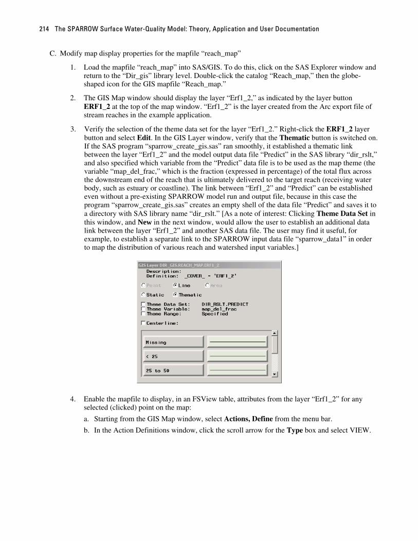
3. Verify the selection of the theme data set for the layer “Erf1_2.” Right-click the ERF1_2 layer button and select Edit. In the GIS Layer window, verify that the Thematic button is switched on. If the SAS program “sparrow_create_gis.sas” ran smoothly, it established a thematic link between the layer “Erf1_2” and the model output data file “Predict” in the SAS library “dir_rslt,” and also specified which variable from the “Predict” data file is to be used as the map theme (the variable “map_del_frac,” which is the fraction (expressed in percentage) of the total flux across the downstream end of the reach that is ultimately delivered to the target reach (receiving water body, such as estuary or coastline). The link between “Erf1_2” and “Predict” can be established even without a pre-existing SPARROW model run and output file, because in this case the program “sparrow_create_gis.sas” creates an empty shell of the data file “Predict” and saves it to a directory with SAS library name “dir_rslt.” [As a note of interest: Clicking Theme Data Set in this window, and New in the next window, would allow the user to establish an additional data link between the layer “Erf1_2” and another SAS data file. The user may find it useful, for example, to establish a separate link to the SPARROW input data file “sparrow_data1” in order to map the distribution of various reach and watershed input variables.]

4. Enable the mapfile to display, in an FSView table, attributes from the layer “Erf1_2” for any selected (clicked) point on the map:

a. Starting from the GIS Map window, select Actions, Define from the menu bar.

b. In the Action Definitions window, click the scroll arrow for the Type box and select VIEW.


c. The field Data Link will appear below the Type field, with PREDICT displayed in the list box. PREDICT is the link (created and named during the execution of the “sparrow_create_gis.sas”) between the attribute data set “Predict” and the layer “Erf1_2.” Examine the link definition by clicking the right-arrow button on the Data Link box: the Attribute Data Sets window displays variables from the data file “Predict” in the Data Set Vars box and variables from the spatial data set in the Composites box. This link specifies that when points are clicked on the mapfile, the FSView table will display attribute values from these two data: the variables (both named arcid) used to link the two data sets are highlighted in each box. Click Continue to accept this link definition.

d. Save by clicking Save then Close.

e. Right-click the ERF1_2 layer button at the top of the map window and select Make Layer Selectable.

5. Select background color for the map (optional formatting):

a. Starting from the GIS Map window, select Tools, Map Properties, Colors.

b. In the Map Styles and Colors window, click the down-arrow control on the Background box to specify a standard color. For custom color (RGB) selection, click the right-arrow control on the Background box and either use the RGB color sliders or type the predefined SAS 8-digit color name (for example CXE1E9DA for beige) in the Name box.


216

c. Save these settings by clicking OK and Close.

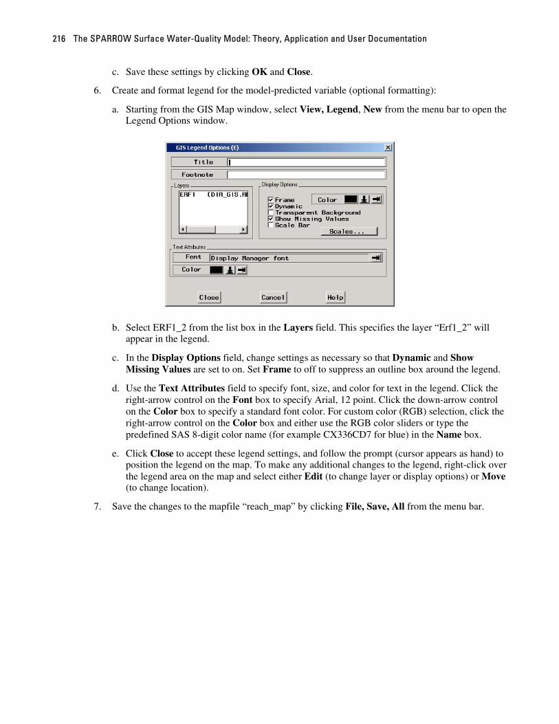
6. Create and format legend for the model-predicted variable (optional formatting):

a. Starting from the GIS Map window, select View, Legend, New from the menu bar to open the Legend Options window.

b. Select ERF1_2 from the list box in the Layers field. This specifies the layer “Erf1_2” will appear in the legend.

c. In the Display Options field, change settings as necessary so that Dynamic and Show Missing Values are set to on. Set Frame to off to suppress an outline box around the legend.

d. Use the Text Attributes field to specify font, size, and color for text in the legend. Click the right-arrow control on the Font box to specify Arial, 12 point. Click the down-arrow control on the Color box to specify a standard font color. For custom color (RGB) selection, click the right-arrow control on the Color box and either use the RGB color sliders or type the predefined SAS 8-digit color name (for example CX336CD7 for blue) in the Name box.

e. Click Close to accept these legend settings, and follow the prompt (cursor appears as hand) to position the legend on the map. To make any additional changes to the legend, right-click over the legend area on the map and select either Edit (to change layer or display options) or Move (to change location).

7. Save the changes to the mapfile “reach_map” by clicking File, Save, All from the menu bar.

Appendix D. Description of Output Files 217

APPENDIX D. Descriptions of Output Files

D.1 Estimation Output File “summary_betaest” (standard if estimation requested) A summary of the structure and function of this file is given in section 2.8.1.4, “Estimation output data

files.”

Description of variables in the file “summary_betaest”

[coefficient_name_k] The parametric estimate of the kth coefficient (of K total coefficients) in the SPARROW model. The name [coefficient_name_k] corresponds to the kth coefficient specified in the betailst control variable in the control file.

(Continue [coefficient_name_1] through [coefficient_name_K])

SD_[coefficient_name_k] The parametric estimate of the standard deviation of the kth coefficient (of K total coefficients) in the SPARROW model. [coefficient_name_k] refers to the kth coefficient specified in the betailst control variable in the control file. Note that the standard deviation is only valid asymptotically.

(Continue SD_[coefficient_name_1] through SD_[coefficient_name_K])

MEAN_EXP_WEIGHTED_ERROR

The mean of the exponentially transformed, weighted model residuals, ( )ˆexp /(1 )i i ie w h− , where

is the estimated residual for the ith observation, is the observation’s leverage, and is the

observation’s weight. This statistic is used to correct for retransformation bias associated with model error in converting results in natural logarithm space to real space.

ie ih iw

VAR_EXP_WEIGHTED_ERROR

The variance of the exponentially transformed weighted model residuals, ( )ˆexp /(1 )i i ie w h− , where

is the estimated residual for the ith observation, is the observation’s leverage, and is the

observation’s weight. This statistic is used to compute standard errors for model predictions expressed in real space.

ie ih iw

NOBS The number of observations used in model estimation.

DF_ERROR The degrees of freedom associated with the model error. This equals the number of observations minus the number of estimated coefficients.

DF_MODEL The degrees of freedom associated with the coefficient estimates. This equals the number of estimated coefficients in the model. Note that constrained coefficients are not included in this statistic.

SSE

The sum of squares of the weighted model residuals, ie wi , where is the estimated residual for

the ith observation and is the observation’s weight.

ie

iw


218


MSE The mean squared error of the SPARROW model, computed by dividing SSE by DF_ERROR.

RMSE The root mean squared error of the SPARROW model, computed as the square root of MSE. This statistic, multiplied by 100, can be interpreted as the one standard deviation percent error associated with a prediction for any single reach (see section 1.5.6).

R_SQUARE The statistic for the logarithm form of the estimated model. The statistic is equal to 2R

( )( )c1 SSE SSQ ln flux− , where SSQc is the sum of squares of the centered values of its argument. Note

that because the SPARROW model does not generally have an intercept, there is no guarantee that this statistic will be between 0 and 1.

ADJ_R_SQUARE The statistic adjusted for the degrees of freedom in the model. The statistic is equal to 2R

( )( )21 1 NOBS 1 DF_ERRORR− − − .

R_SQ_YLD The statistic for the logarithm of yield form of the model. The statistic is equal to 2R

( )( )c1 SSE SSQ ln yield− , where SSQc(ln(yield) is the sum of squares of the centered values of the

natural logarithm of yield. Note that because a SPARROW model does not generally have an intercept, there is no guarantee that this statistic will be between 0 and 1. This statistic generally will

have a value that is lower than the statistic. 2R

E_VAL_SPREAD The eigenvalue spread. The eigenvalues are determined from the X X′ matrix, where X is the matrix of coefficient gradients, normalized by the square root of the sum of squares of the gradients for each coefficient (see section 1.5.4.3). If the SPARROW model includes an intercept, the gradients are

centered prior to computing X . The spread equals the maximum eigenvalue divided by the minimum eigenvalue. Eigenvalue spreads greater than 100 indicate a potential problem due to multicollinearity.

PPCC The probability plot correlation coefficient. The statistic is the correlation between the standardized

weighted model residual, ( )2ˆ 1i i i ie e w s h∗ = −

)

, and the inverse normal value of the residual’s rank,

( )( ) ((1 .4 .2irank e N− ∗Φ − )+ , where is the weight for observation i, is the model residual

for observation i (expressed in natural logarithm units), is the mean-squared error of the weighted

model residual, is the observation i leverage statistic,

iw ie2s

ih ( )1−Φ ⋅ is the inverse of the standard normal

cumulative distribution function, and N is the number of observations (see section 1.5.5.1). A value near one indicates the weighted residuals are approximately normally distributed.



SWILK_STAT The Shapiro-Wilks test statistic for testing the assumption of normally distributed weighted residuals

ie wi , where is the estimated residual for the ith observation and is the observation’s weight.

The statistic may be interpreted as the squared correlation coefficient between the ordered values of the weighted residuals and the corresponding order statistics generated from a standard normal distribution, appropriately adjusted for covariance between the order statistics (see section 1.5.5.1). A small value for the statistic implies a low correlation and is indicative of a departure from normality.

ie iw

SWILK_PVAL The probability value for the Shapiro-Wilks test statistic evaluating the normality of the weighted

residuals ie wi , where is the estimated residual for the ith observation and is the observation’s

weight. The p-value is between 0 and 1, with values less than 0.05 implying the assumption of normality of the residuals is rejected at a significance level of 5 percent.

ie iw

UNBIAS_[coefficient_name_k] (optional) The bootstrap estimate of the unbiased value of the kth coefficient (of K total coefficients) in the model. The estimate is equal to two times the parametric estimate minus the mean of the bootstrap estimates (see section 1.5.3.1). [coefficient_name_k] corresponds to the kth coefficient specified in the betailst control variable in the control file. This variable appears only if bootstrapping is requested by setting a non-zero value for the n_boot_iter control variable in the control file.

(Continue UNBIAS_[coefficient_name_1] through UNBIAS_[coefficient_name_K])

STDEV_[coefficient_name_k] (optional) The bootstrap estimate of the standard deviation of the kth coefficient (of K total coefficients) in the model. The estimate is equal to the square root of the variance of the bootstrap estimates (see section 1.5.3.2). [coefficient_name_k] corresponds to the kth coefficient specified in the betailst control variable in the control file. This variable appears only if bootstrapping is requested by setting a non-zero value for the n_boot_iter control variable in the control file.

(Continue STDEV_[coefficient_name_1] through STDEV_[coefficient_name_K])

CI_LO_[coefficient_name_k] (optional) The bootstrap estimate of the lower bound on the confidence interval for the kth coefficient in the model (of K total coefficients). The lower bound estimate is equal to two times the parametric coefficient estimate minus the rth lowest value of the bootstrap estimates, with

( ) ( )1 2 1r B p B p B⎢ ⎥ ⎢= + − − −⎣ ⎦ ⎣ ⎥⎦ , where ⎢ ⎥⎣ ⎦ is the floor function representing the largest integer

that is less than or equal to the function’s argument, p is the coverage probability given by the cov_prob control variable (divided by 100), and B is the number of bootstrap iterations defined by the n_boot_iter control variable (see section 1.5.3.3). [coefficient_name_k] corresponds to the kth coefficient specified in the betailst control variable in the control file. This variable appears only if bootstrapping is requested by setting a non-zero value for the n_boot_iter control variable in the control file.

(Continue CI_LO_[coefficient_name_1] through CI_LO_[coefficient_name_K])


220


CI_HI_[coefficient_name_k] (optional) The bootstrap estimate of the upper bound on the confidence interval for the kth coefficient in the model (of K total coefficients). The upper bound estimate is equal to two times the parametric

coefficient estimate minus the rth lowest value of the bootstrap estimates, with ( )1 2r p B⎢ ⎥= − +⎣ ⎦ 1 ,

where is the floor function representing the largest integer that is less than or equal to the

function’s argument, p is the coverage probability given by the cov_prob control variable (divided by 100), and B is the number of bootstrap iterations defined by the n_boot_iter control variable (see section 1.5.3.3). [coefficient_name_k] corresponds to the kth coefficient specified in the betailst control variable in the control file. This variable appears only if bootstrapping is requested by setting a non-zero value for the n_boot_iter control variable in the control file.

⎢ ⎥⎣ ⎦

(Continue CI_HI_[coefficient_name_1] through CI_HI_[coefficient_name_K])


D.2 Estimation Output File “cov_betaest” (standard if estimation requested) A summary of the structure and function of this file is given in section 2.8.1.4, “Estimation output data

files.” Note that each row of the “cov_betaest” file corresponds to one of the coefficients declared in the betailst control variable, appearing in the same order as the coefficients are listed across the columns of the “cov_betaest” file.

Description of variables in the file “cov_betaest”

[coefficient_name_k] The parametric covariances for the kth coefficient (of K total coefficients) in the SPARROW model. [coefficient_name_k] corresponds to the kth coefficient name specified in the betailst control variable in the control file. Note that the covariance estimates are only valid asymptotically (see section 1.5.1.3).


VIF The variance inflation factor for each coefficient. The square root of the variance inflation factor is equal to the proportion by which the coefficient’s t-statistic could be increased if multicollinearity was eliminated (that is, if the gradient associated with the coefficient was orthogonal to the gradients of all the other coefficients in the model) (see section 1.5.4.3).

E_VAL The eigenvalue for each coefficient. The eigenvalues are determined from the X X′ matrix, where X is the matrix of coefficient gradients, normalized by the square root of the sum of squares of the gradients for each coefficient. If the SPARROW model includes an intercept, the gradients are

centered prior to computing X (see section 1.5.4.3).


222

D.3 Estimation Output File “resids” (standard if estimation requested) A summary of the structure and function of this file is given in section 2.8.1.4, “Estimation output data

files.”

Description of variables in the file “resids”

[station_identifier] The station identification code. [station_identifier] is the name of the variable defined by the control variable staid in the control file. This variable must be numeric.

[station_ancillary_variable_n] (optional) nth ancillary variable (of N total ancillary variables) defined in the control variable optional_station_information in the control file. Ancillary station variables are included only if the optional_station_information control variable is not blank. Ancillary station variables can be character or numeric.

(Continue [station_ancillary_variable_1] through [station_ancillary_variable_N])

[station_longitude] The station longitude, expressed in decimal degrees. [station_longitude] is the name of the variable defined by the control variable lon in the control file. The longitude value is negative for locations in the Western Hemisphere.

[station_latitude] The station latitude, expressed in decimal degrees. [station_latitude] is the name of the variable defined by the control variable lat in the control file.

[reach_identifier] The reach identification code for the reach in which the station is located. [reach_identifier] is the name of the variable defined by the control variable waterid in the control file. The variable must be numeric.

[arc_identifier] (optional) The identification number for linking to the ARC coverage imported into SAS/GIS for the spatial display of residuals. [arc_identifier] is the name of the variable defined by the control variable arcid in the control file. The specification of this control variable is optional.

[least_squares_weight] The weight used in the least squares model estimation. [least-squares-weight] is the name of the variable defined by the control variable ls_weight in the control file. Prior to model estimation, each weight is automatically normalized by dividing by the mean of the weights for all observations. If no preferential weighting is required, the variable should have equivalent values for all observations.

ACTUAL The monitored flux, expressed in units of kilograms year-1 (kg/yr), metric tons year-1 (mt/yr), or billion-colonies year-1 (Bcol/yr) depending on the specification of the control variable load_units in the control file.



PREDICT The predicted flux at monitoring stations, expressed in units of kg/yr, mt/yr or Bcol/yr depending on the specification of the control variable load_units in the control file. The predicted flux is computed by accumulating the contaminant sources delivered to streams and applying the in-stream and reservoir attenuation processes (see section 1.4.1). The prediction is not adjusted for retransformation bias. All processes are evaluated using the parametric estimates of the coefficients. Moreover, the predictions are contingent on upstream monitored flux (regardless of the specification of the if_adjust control variable—see section 2.6.3.7). That is, in accumulating predicted flux in the downstream direction, if a reach has a monitored flux, the monitored value is substituted for the predicted value in the amount of flux delivered to the reach’s downstream node. This does not affect the prediction for the monitored reach but it does affect the predictions for all reaches downstream from the monitored reach.

LN_ACTUAL The natural logarithm of the monitored flux, ACTUAL.

LN_PREDICT The natural logarithm of the predicted flux, PREDICT.

LN_PRED_YIELD The natural logarithm of predicted yield. The variable equals LN_PREDICT minus the natural logarithm of the drainage area for the monitored reach. The variable representing drainage area is defined by the control variable tot_area.

LN_RESID The estimated model residual, expressed in natural logarithm units. The residual is equal to the difference between LN_ACTUAL and LN_PREDICT.

WEIGHTED_LN_RESID The weighted model residual, expressed in natural logarithm units. The weighted model residual

equals ie wi , where is the model residual LN_RESID and is the least squares weight

([ls_weight]), the variable defined by the control variable ls_weight. ie iw

MAP_RESID The Studentized residual, used to generate the spatial map of model residuals. The Studentized

residual is equal to ( )2ˆ 1i i ie w s h− , where is the model residual LN_RESID, is the least

squares weight defined by the control variable ls_weight, is the mean squared error of the model (MSE) – the sum of squares of the weighted residual WEIGHTED_LN_RESID divided by the number of degrees of freedom for the model (NOBS minus DF_MODEL), and is the leverage for

the observation (see the LEVERAGE variable defined below). By assumption, the effect of weighting makes the underlying model residual homoscedastic. For linear models, the adjustment for the leverage causes the estimated residuals to have equal variance across all observations. For the nonlinear model, the leverage statistic is formed from the model gradients (see section 1.5.1.4). In this case, the leverage adjustment is justified by assuming that the gradients for each observation have proportional representation in extending the sample to infinity. Finally, normalization by the root mean squared error causes each residual to have unit variance. The Studentized normalization of the residuals provides a general scale for evaluating the magnitude of the residuals. Values of the Studentized residual greater than 3.6 are generally considered outliers and warrant further investigation.

ie iw2s

ih


224


BOOT_RESID The weighted residual used for computing the Smearing estimator of the retransformation bias

adjustment factor. The weighted residual is equal to ( )ˆ 1i i ie w h− , where is the model residual

LN_RESID, is the least squares weight defined by the control variable ls_weight, and is the

leverage statistic (see LEVERAGE below). The mean of the exponential transform of these residuals represents the retransformation bias adjustment factor (see section 1.6.2). The variance of the exponential transform of these residuals defines the model-error component of the prediction error (see section 1.6.4)

ie

iw ih

LEVERAGE The leverage statistic for each observation. The leverage statistic represents the influence the given observation has on model estimation. An observation with a large leverage statistic implies the value of the dependent variable for that observation has a large effect on that observation’s prediction. In

the context of a linear model, the leverage statistic is equal to ( ) 1i ix X X x

−′ ′ , where ix is the vector

of values of the explanatory variables for observation i and X is the matrix of explanatory variables for all observations in the regression. If the linear model has an intercept, a large leverage statistic indicates the values of the explanatory variables for the observation differ substantially from the mean values of the explanatory variables for the entire regression. Consequently, such an observation has a large effect on the determination of the coefficient estimates. The sum of the leverage statistics across all observations equals the number of estimated coefficients in the model. Therefore, in a linear model, observations with a leverage statistic greater than DF_MODEL/NOBS are relatively more influential. In the context of a nonlinear model, the leverage statistic is computed using the model gradients (see the description below of the variables containing the gradient for each model coefficient) in place of ix and X. The statistical properties of a nonlinear model are generally defined

only for large samples. In large samples, however, the leverage statistic for any given observation goes to zero, implying the influence of any single observation is of no consequence. The leverage statistic has practical relevance in a nonlinear model if it is assumed that large samples are obtained by reproducing the observed set of explanatory variables in repeated samples. Under this interpretation, an observation with a leverage statistic greater than DF_MODEL/NOBS is representative of a non-negligible group of observations that collectively have a larger influence on model estimation than other observation groups (see section 1.5.1.4).

Z_MAP_RESID The normal quantile of the offset rank of the Studentized residual used to generate the probability plot gbt_prob_plot and the probability plot correlation coefficient PPCC. The variable is equal to

( )( ) ( )( ) (1 rank .4 .2ie N− ∗Φ − + , where )1− ⋅Φ is the inverse of the normal cumulative distribution

function, is the rank of the observation’s Studentized residual (MAP_RESID), and N is

the number of observations (NOBS) (see section 1.5.5.1).

( )rank ie∗



[coefficient_name_k] The gradient for the kth model coefficient (of K total coefficients). The gradient is the derivative of the weighted squared residual with respect to the named coefficient (see section 1.5.1.2). In SPARROW, the gradients are computed numerically by evaluating the change induced in a model prediction (LN_PREDICT) from a small change in one of the coefficient estimates (see section 1.5.1.5). The gradients can be used to compute the leverage statistics and perform non-nested hypothesis tests. [coefficient_name_k] represents the kth coefficient identified by the betailst control variable in the control file.


id A sequential identifier, assigned by SPARROW to facilitate the referencing of monitoring sites.


226

D.4 Estimation Output File “boot_betaest_all” (standard if estimation requested) A summary of the structure and function of this file is given in section 2.8.1.4, “Estimation output data

files.”

Description of variables in the file “boot_betaest_all”

iter The bootstrap iteration number. Iteration 0 pertains to the parametric estimates.

jter The bootstrap random seed index number. The value for jter could exceed iter if the estimation of the model fails for some randomly selected resampling of the observations, in which case the iteration estimates are obtained by drawing a new set of random variables.

[coefficient_name_k] The estimate of the kth coefficient (of K total coefficients) in the SPARROW model. [coefficient_name_k] corresponds to the kth name specified in the betailst control variable in the control file and are in the same order.


mean_exp_weighted_error

The mean of the exponentially transformed, weighted model residuals, ( )ˆexp /(1 )i i ie w h− , where

is the estimated residual for the ith observation as obtained from the iter-th bootstrap sample,

is the observation’s leverage, and is the observation’s weight. This statistic is used to correct for

retransformation bias associated with model error in converting results in natural logarithm space to real space.

ie ih

iw


D.5 Estimation Output File “test_resids” (optional) A summary of the structure and function of this file is given in section 2.8.1.4, “Estimation output data files.”

Description of variables in the file “test_resids”

[waterid] The reach identification code for the reach in which the station is located. [waterid] is the name of the variable defined by the control variable waterid. The variable must be numeric.

[staid] The station identification code. [staid] is the name of the variable defined by the control variable staid.

ACTUAL The monitored flux, expressed in units of kilograms year-1 (kg/yr), metric tons year-1 (mt/yr), or billion colonies year-1 (Bcol/yr) depending on the specification of the control variable load_units in the control file.

PREDICT The predicted flux at monitoring stations, expressed in units of kg/yr, mt/yr or Bcol/yr depending on the specification of the control variable load_units in the control file. For a description of how this variable is computed, see the discussion above (appendix D.3) of the variable PREDICT in the “resids” file. For monitored reaches for which computed flux is nonpositive (due to numerical overflow in model computation for an upstream reach), the value for ACTUAL is reported in place of PREDICT.

LN_ACTUAL The natural logarithm of the monitored flux, ACTUAL.

LN_PREDICT The natural logarithm of the predicted flux, PREDICT, or for monitored reaches for which computed flux is nonpositive, the value for LN_ACTUAL is reported in place of LN_PREDICT.

LN_PRED_YIELD The natural logarithm of predicted yield. The variable equals LN_PREDICT minus the natural logarithm of the drainage area for the monitored reach. The variable representing drainage area is defined by the control variable tot_area.

LN_RESID The estimated model residual, expressed in natural logarithm units. For monitored reaches with a nonpositive value of the predicted flux (that is, PREDICT is less than or equal to zero) the value of LN_RESID is set equal to zero. Otherwise, the residual is equal to the difference between LN_ACTUAL and LN_PREDICT.

WEIGHTED_LN_RESID The weighted model residual, expressed in natural logarithm units. For monitored reaches with a nonpositive value of the predicted flux (that is, PREDICT is less than or equal to zero) the value of

WEIGHTED_LN_RESID is set to zero. Otherwise, the weighted model residual equals ie wi , where

is the model residual LN_RESID and is the least squares weight ([ls_weight]), the variable

defined by the control variable ls_weight. ie iw

N_RCH The number of reaches making up the station’s nested basin. That is, the number of reaches upstream of the given monitoring station (including the monitored reach) and below any upstream monitoring station.


228

D.6 Prediction Output File “predict” (standard if prediction requested) All variables are defined in detail in the table at the end of this section. The following discussion explains

naming conventions for the variables and discusses special considerations for bias-adjusted estimates, confidence intervals, reservoir and reach decay, and delivery fraction.

Predictions are given for total flux and flux by source. Predictions of total flux have the suffix TOTAL and predictions for a topical source have the suffix [source_k], where [source_k] refers to the kth source variable defined by the control variable srcvar. Flux predictions are also reported for three constitutions: the amount of flux exported from the reach, the amount exported from the reach if there was no in-stream or reservoir attenuation, and the amount of flux leaving the reach that was generated within the reach’s incremental watershed. Additionally, the predictions include an estimate of the accumulated amount of flux removed from the stream network from reservoirs at and upstream of the given reach. If the control variable target is specified, the predictions contain an estimate of the fraction of flux leaving the reach that is delivered to the outlet of the nearest downstream target reach.

All predictions having the prefix PLOAD_ in their name are based on parametric estimates of the coefficients—the coefficients obtained from model estimation using the full original sample of observations. These predictions have been corrected for retransformation bias in the model residuals but not in the coefficient sampling error (see section 1.6.2). The adjustment for retransformation bias uses a Smearing estimator evaluated using the weighted estimated residuals, adjusted for the leverage of the observation (see section 1.6.2). Note that the same retransformation bias adjustment factor is applied to all flux predictions, regardless of source, location, or constitution (that is, exported, non-decayed, or incremental). Additionally, the retransformation bias adjustment factor is applied to the predicted amount of flux removed in reservoirs. However, the factor is not applied to prediction variables that are declared in the control variable retrans_exclude_list. These variables, for example the delivery fraction variable, are not denominated in units of flux so the model error is not included in their estimation (see section 1.6.6).

Predictions having the prefix MEAN_PLOAD_ are based on a bootstrap analysis in conjunction with the parametric estimates to obtain a bootstrap estimate that is corrected for both the retransformation bias due to model error and the nonlinear prediction bias caused by sampling error in the coefficient estimates. The method of correction for nonlinear bias caused by sampling error is to generate multiple model prediction estimates using multiple sets of coefficient estimates obtained either from resampled data or from randomly generated coefficient vectors using a normal random number generator (see section 1.5.3.1). A proportional nonlinear bias adjustment factor is computed by dividing the parametric prediction by the average of the multiple bootstrap model predictions (see section 1.6.3). The ratio form of the bias adjustment factor insures that the restrictions placed on the coefficients to guarantee that flux predictions are positive will hold for the bias-adjusted estimate (that is, will result in a positive bias-adjusted estimate). A consequence of this adjustment, however, is that mass balance restrictions across prediction variables no longer hold. For example, whereas the parametric predictions described above restrict the sum of predicted flux by source to equal total flux, predictions that have been adjusted using the proportional bias adjustment factor no longer retain that restriction. The restriction can instead be imposed in user post-processing of model output, by computing the estimates of bias-adjusted individual source shares of flux estimates as a function of total bias-adjusted flux, or vice versa. For example, one approach is to allocate the bias-adjusted prediction of total flux to the individual sources based on the share of flux from each source estimated from the parametric predictions. A second approach is to set the total bias-adjusted flux to equal the sum of the individual source bias adjusted flux. Or third, the bias-adjusted prediction of total flux can be allocated to the individual sources based on the ratio of the bias-adjusted source estimates to the total of the bias-adjusted source estimates.

Bootstrap-derived standard error estimates of the predictions are contained in variables having the prefix SE_PLOAD_. The standard errors reflect variability due to sampling error in the coefficient estimates and variability arising from model error (see section 1.6.4). The standard errors for prediction variables included in the retrans_exclude_list reflect only the variance caused by sampling error in the coefficient estimates; the variance due to model error is excluded.

Prediction variables with the prefix CI_LO_ and CI_HI_ represent the estimate’s lower and upper bounds on an equal-tailed confidence interval. The coverage probability for the interval, p, is defined by the control variable cov_prob. The confidence interval is based on bootstrap methods, and expresses the lower and


upper bounds as a ratio between the square of the parametric prediction and the appropriate order statistic from the bootstrap simulations (see section 1.6.5). The ratio form used to derive the lower and upper bounds insures that the bounds are strictly positive for positive source variables. The randomly selected weighted model residual is not included for prediction variables defined by the control variable retrans_exclude_list.

Prediction variables with the prefix PLOAD_ND_ or MEAN_PLOAD_ND_ refer to estimates of flux that would have left the reach if there were no in-stream or reservoir attenuation processes (ND denotes “No Decay”). Therefore the difference between the predicted “no-decay” flux and predicted flux represents the amount of flux reaching streams, including and upstream of the given reach, that is removed from the outflow of the reach due to in-stream and reservoir attenuation processes.

Prediction variables with the prefix PLOAD_INC_ and MEAN_PLOAD_INC_ refer to estimates of flux leaving the reach that are generated within the incremental reach watershed. The predicted flux represents the amount of flux delivered to the reach from sources within the reach’s incremental watershed (by the given source if the suffix consists of a source name) and attenuated by reservoir and in-stream processes within the same reach. If the reach is a reservoir reach, the reach’s full reservoir attenuation process is applied to the delivered flux. If the reach is not a reservoir, the incremental watershed flux is assumed to enter the reach at the reach’s midpoint and receives only a portion of the reach’s in-stream attenuation (the reach delivery factor for incremental watershed flux is the square root of the reach delivery factor applied to flux from an upstream reach).

The variable RES_DECAY and MEAN_RES_DECAY correspond to the amount of flux removed from the reach network through reservoir attenuation. That is, these variables represent the change in the amount of flux leaving the reach if all reservoirs at or upstream of the reach were removed from the network. A non-zero value is reported only if a resevoir attenuation process is defined in the control variable reservoir_decay_specification. Although the predictions do not include a direct estimate, the flux removed due to in-stream attenuation can be estimated by taking the difference between PLOAD_ND_TOTAL and the sum of RES_DECAY and PLOAD_TOTAL (or by the difference between MEAN_PLOAD_ND_TOTAL and the sum of MEAN_RES_DECAY and MEAN_PLOAD_TOTAL).

The variables DEL_FRAC and MEAN_DEL_FRAC represent the parametric and bias-adjusted estimates of the share of flux leaving the reach that is delivered to the outlet of the nearest downstream target reach (see section 1.6.7), as identified by the variable defined by the control variable target. The variable DEL_FRAC should be listed in the retrans_exclude control variable to preclude application of the retransformation bias adjustment. The prediction variable MAP_DEL_FRAC is the DEL_FRAC variable expressed in percent. This variable is included in the output to support the generation of the default reach map in SAS/GIS. The amount of flux generated in the reach and delivered to the outlet of the nearest downstream target reach can be estimated as a post-processing step by multiplying the predicted incremental watershed flux (prediction variables with the prefix PLOAD_INC_ and MEAN_PLOAD_INC_) by DEL_FRAC.

If the control variable if_adjust is set to yes, all predictions at and downstream of monitored reaches are conditioned on the monitored flux—meaning that the monitored flux is substituted for the predicted flux at those reaches, this monitored value being used in the subsequent predictions of downstream flux. For a monitored reach, the conditioning of predicted flux on monitored flux causes the standard error of the total flux estimate to be set to zero and the source shares for the reach are derived by applying the predicted source share times the monitored flux. For simulation of alternative water management scenarios it is generally the case that if_adjust is set to no. Note that the predictions for a reach immediately downstream of a monitored reach receive an adjustment to account for retransformation bias arising from the expectation of the multiplicative error term; with if_adjust set to yes, the measured flux at a monitored reach receives no such adjustment because the error (rather than its expectation) is assumed to be incorporated directly in the flux measurement (see section 1.6.6).


230

Description of variables in the file “predict” (preceding text contains additional explanations)

[reach_identifier] The reach identification code. [reach_identifier] is the name of the variable defined by the control variable waterid in the control file. The variable must be numeric.

[reach_ancillary_variable_n] The nth ancillary variable (of N total ancillary variables) defined in the control variable optional_reach_information. Ancillary reach variables are included only if the optional_reach_information control variable is not blank. Ancillary reach variables can be character or numeric.

(Continue [reach_ancillary_variable_1] through [reach_ancillary_variable_N])

[station_identifier] The station identification code. [station_identifier] is the name of the variable defined by the control variable staid in the control file. This variable must be numeric.

[tot_area] (kilometers2, km2) The total area upstream of the reach outlet, in units of kilometers2 (km2). [tot_area] is the name of the variable defined by the control variable tot_area.

[inc_area] (kilometers2, km2) The incremental watershed area, in units of km2. [inc_area] is the name of the variable defined by the control variable inc_area.

[mean_flow] (feet3 second-1, ft3/s, or 100 liters second-1, 100 L/s) The mean flow of the reach. [mean_flow] is the name of the variable defined by the control variable mean_flow. Units are either feet3 second-1 (ft3/s) or 100 liters second-1 (100 L/s) as defined by the control variable flow_units.

[arc_identifier] (optional) The idenfication number for linking to the ARC coverage imported into SAS/GIS for the spatial display of residuals. [arc_identifier] is the name of the variable defined by the control variable arcid in the control file. The specification of this control variable is optional.

[from_node] The upstream node of the reach. [from_node] is the name of the variable defined by the control variable fnode.

[to_node] The downstream node of the reach. [to_node] is the name of the variable defined by the control variable tnode.

[hydseq] The hydrologic sequence of reaches in the network. [hydseq] is the name of the variable defined by the control variable hydseq. Sorting the SAS input data set by [hydseq] in ascending order facilitates the sequential accumulation of flux—the incremental flux for any reach is not accumulated until the incremental fluxes from all upstream reaches have been accumulated.

[frac] The fraction of upstream flux diverted to the reach. [frac] is the name of the variable defined by the control variable frac. The value of [frac] for a reach is less than one only if there is a diversion at the upstream node.



[iftran] The variable determining if flux is delivered through the reach to the downstream node. [iftran] is the name of the variable defined by the control variable iftran.

[target] Target classification (0/1) of the reach. [target] is the name of the variable identified by the control variable target.

[least_squares_weight] The weight used in the least squares model estimation. [least_squares_weight] is the name of the variable defined by the control variable ls_weight in the control file. Prior to model estimation, each weight is automatically normalized by dividing by the mean of the weights for all observations. If no preferential weighting is required, the variable should have equivalent values for all observations.

LU_class Land use classification for the reach. A value is reported for the reaches that meet one of the criteria defined in the control variable land_class_list (that is, for the reaches that will be included in the statistical summary of yield by land use). LU_class is blank for reaches that do not meet any of the criteria. The values recorded for this variable are the class names defined in the land_class_list control variable. The variable LU_class is included in the output file only if the control variable if_distribute_yield_by_land_use is set to yes.

[depvar] (kilograms year-1 (kg/yr), metric tons year-1 (mt/yr), or billion colonies year-1 (Bcol/yr)) The monitored flux. [depvar] is the name of the variable defined by the control variable depvar. The units are defined by the control variable load_units and may be kilograms year-1 (kg/yr), metric tons year-1 (mt/yr), or billion colonies year-1 (Bcol/yr).

PLOAD_TOTAL (kg/yr, mt/yr or Bcol/yr) Predicted total flux leaving the reach. Estimates are corrected for retransformation bias caused by the model residuals but are not corrected for bias caused by sampling error in the coefficient estimates. The units are defined by the control variable load_units and may be kg/yr, mt/yr or Bcol/yr.

PLOAD_[source_s] (kg/yr, mt/yr or Bcol/yr) Predicted flux leaving the reach attributed to the sth source (of S total sources) in the SPARROW model. Estimates are corrected for retransformation bias caused by the model residuals but are not corrected for bias caused by sampling error in the coefficient estimates. [source_s] is the sth source defined in the control variable srcvar. The units are defined in the control variable load_units and may be kg/yr, mt/yr or Bcol/yr.

(Continue PLOAD_[source_1] through PLOAD_[source_S])

PLOAD_ND_TOTAL (kg/yr, mt/yr or Bcol/yr) Predicted total flux leaving the reach if there are no in-stream or reservoir attenuation processes. Estimates are corrected for retransformation bias caused by the model residuals but are not corrected for bias caused by sampling error in the coefficient estimates. The units are defined in the control variable load_units and may be kg/yr, mt/yr or Bcol/yr.

PLOAD_ND_[source_s] (kg/yr, mt/yr or Bcol/yr) Predicted flux attributed to the sth source (of S total sources) in the model that leaves the reach assuming no in-stream or reservoir attenuation processes. Estimates are corrected for retransformation bias caused by the model residuals but are not corrected for bias caused by sampling error in the coefficient estimates. [source_s] is the sth source defined by the control variable srcvar. The units are defined in the control variable load_units and may be kg/yr, mt/yr or Bcol/yr.


232


(Continue PLOAD_ND_[source_1] through PLOAD_ND_[source_S])

PLOAD_INC_TOTAL (kg/yr, mt/yr or Bcol/yr) Predicted total flux generated within the reach’s incremental watershed. Estimates receive an adjustment for stream attenuation within the reach (see preceeding text for details). Estimates are corrected for retransformation bias caused by the model residuals but are not corrected for bias caused by sampling error in the coefficient estimates. The units are defined in the control variable load_units and may be kg/yr, mt/yr or Bcol/yr.

PLOAD_INC_[source_s] (kg/yr, mt/yr or Bcol/yr) Predicted total flux generated within the reach’s incremental watershed and attributed to the sth source in the model. [source_s] is the sth variable defined in the control variable srcvar. Estimates receive an adjustment for stream attenuation within the reach (see preceeding text for details). Estimates are corrected for retransformation bias caused by the model residuals but are not corrected for bias caused by sampling error in the coefficient estimates. The units are defined in the control variable load_units and may be kg/yr, mt/yr or Bcol/yr.

(Continue PLOAD_INC_[source_1] through PLOAD_INC_[source_S])

RES_DECAY (kg/yr, mt/yr or Bcol/yr) The amount that total flux leaving the reach is reduced because of reservoir attenuation within and upstream of the given reach. Estimates are corrected for retransformation bias caused by the model residuals but are not corrected for bias caused by sampling error in the coefficient estimates. The value is zero if no reservoir attenuation process is specified in the control variable reservoir_decay_specification.The units are defined in the control variable load_units and may be kg/yr, mt/yr or Bcol/yr.

DEL_FRAC (unitless) The fraction of flux leaving the reach that is delivered to the nearest downstream target reach. Because the predicted variable is not a flux, the estimate does not receive an adjustment for retransformation bias. If in-stream and reservoir processes are restricted to be attenuating, the predicted value is between zero and one. The value is set to missing if no target variable is defined by the control variable target. The value is set to one if no in-stream or reservoir attenuation processes are specified in the control variables reach_decay_specification and reservoir_decay_specification. The prediction is a fraction and therefore unitless.

MEAN_PLOAD_TOTAL (kg/yr, mt/yr or Bcol/yr) Bootstrap bias-adjusted predicted total flux leaving the reach. Estimates are corrected for retransformation bias caused by the model residuals and nonlinear bias caused by sampling error in the coefficient estimates. The variable is only included if a bootstrap analysis is requested by setting the control variable n_boot_iter to a value greater than zero. The units are defined in the control variable load_units and may be kg/yr, mt/yr or Bcol/yr.

SE_PLOAD_TOTAL (kg/yr, mt/yr or Bcol/yr) Standard error of the predicted total flux leaving the reach. The standard error includes the variation arising from model error and the variation caused by sampling error in the coefficient estimates. The variable is only included if a bootstrap analysis is requested by setting the control variable n_boot_iter to a value greater than zero. The units are defined in the control variable load_units and may be kg/yr, mt/yr or Bcol/yr.



CI_LO_PLOAD_TOTAL (kg/yr, mt/yr or Bcol/yr) Lower bound on the bootstrap-derived confidence interval for the total flux leaving the reach. The coverage probability is defined by the control variable cov_prob. The variable is only included if a bootstrap analysis is requested by setting the control variable n_boot_iter to a value greater than zero. The units are defined by the control variable load_units and may be kg/yr, mt/yr or Bcol/yr.

CI_HI_PLOAD_TOTAL (kg/yr, mt/yr or Bcol/yr) Upper bound on the bootstrap-derived confidence interval for the total flux leaving the reach. The coverage probability is defined by the control variable cov_prob. The variable is only included if a bootstrap analysis is requested by setting the control variable n_boot_iter to a value greater than zero. The units are defined by the control variable load_units and may be kg/yr, mt/yr or Bcol/yr.

MEAN_PLOAD_[source_s] (kg/yr, mt/yr or Bcol/yr) (optional) Bootstrap bias-adjusted predicted flux leaving the reach attributed to the sth source (of S total sources) in the model. [source_s] is the sth source listed in the control variable srcvar. Estimates are corrected for retransformation bias caused by the model residuals and nonlinear bias caused by sampling error in the coefficient estimates. The variable is only included if a bootstrap analysis is requested by setting the control variable n_boot_iter to a value greater than zero. The units are defined in the control variable load_units and may be kg/yr, mt/yr or Bcol/yr.

SE_PLOAD_[source_ s] (kg/yr, mt/yr or Bcol/yr) (optional) Standard error of the predicted flux leaving the reach attributed to the sth source (of S total sources) in the model. [source_ s] is the sth source listed in the control variable srcvar. The standard error includes the variation arising from model error and the variation caused by sampling error in the coefficient estimates. The variable is only included if a bootstrap analysis is requested by setting the control variable n_boot_iter to a value greater than zero. The units are defined in the control variable load_units and may be kg/yr, mt/yr or Bcol/yr.

CI_LO_PLOAD_[source_ s] (kg/yr, mt/yr or Bcol/yr)(optional) Lower bound on the bootstrap-derived confidence interval for flux leaving the reach attributed to the sth source (of S total sources) in the model. [source_ s] is the sth source listed in the control variable srcvar. The coverage probability is defined by the control variable cov_prob. The variable is only included if a bootstrap analysis is requested by setting the control variable n_boot_iter to a value greater than zero. The units are defined by the control variable load_units and may be kg/yr, mt/yr or Bcol/yr.

CI_HI_PLOAD_[source_ s] (kg/yr, mt/yr or Bcol/yr) (optional) Upper bound on the bootstrap-derived confidence interval for flux leaving the reach attributed to the sth source (of S total sources) in the model. [source_ s] is the sth source listed in the control variable srcvar. The coverage probability is defined by the control variable cov_prob. The variable is only included if a bootstrap analysis is requested by setting the control variable n_boot_iter to a value greater than zero. The units are defined by the control variable load_units and may be kg/yr, mt/yr or Bcol/yr.

(Continue MEAN_PLOAD_, SE_PLOAD_, CI_LO_PLOAD_, CI_HI_PLOAD_ [source_1] through MEAN_PLOAD_, SE_PLOAD_, CI_LO_PLOAD_, CI_HI_PLOAD_ [source_S])


234


MEAN_PLOAD_ND_TOTAL (kg/yr, mt/yr or Bcol/yr) (optional) Bootstrap bias-adjusted predicted total flux leaving the reach with in-stream and reservoir attenuation processes “turned off.” Estimates are corrected for retransformation bias caused by the model residuals and nonlinear bias caused by sampling error in the coefficient estimates. The variable is included only if a bootstrap analysis is requested by setting the control variable n_boot_iter to a value greater than zero. The units are defined in the control variable load_units and may be kg/yr, mt/yr or Bcol/yr.

SE_PLOAD_ ND_TOTAL (kg/yr, mt/yr or Bcol/yr) (optional) Standard error of the predicted total flux leaving the reach with in-stream and reservoir attenuation processes “turned off.” The standard error includes the variation arising from model error and the variation caused by sampling error in the coefficient estimates. The variable is included only if a bootstrap analysis is requested by setting the control variable n_boot_iter to a value greater than zero. The units are defined in the control variable load_units and may be kg/yr, mt/yr or Bcol/yr.

CI_LO_PLOAD_ ND_TOTAL (kg/yr, mt/yr or Bcol/yr) (optional) Lower bound on the bootstrap-derived confidence interval for the total flux leaving the reach assuming in-stream and reservoir attenuation processes are “turned off.” The coverage probability is defined by the control variable cov_prob. The variable is included only if a bootstrap analysis is requested by setting the control variable n_boot_iter to a value greater than zero. The units are defined by the control variable load_units and may be kg/yr, mt/yr or Bcol/yr.

CI_HI_PLOAD_ ND_TOTAL (kg/yr, mt/yr or Bcol/yr) (optional) Upper bound on the bootstrap-derived confidence interval for the total flux leaving the reach assuming in-stream and reservoir attenuation processes are “turned off.” The coverage probability is defined by the control variable cov_prob. The variable is included only if a bootstrap analysis is requested by setting the control variable n_boot_iter to a value greater than zero. The units are defined by the control variable load_units and may be kg/yr, mt/yr or Bcol/yr.

MEAN_PLOAD_ ND_ [source_s] (kg/yr, mt/yr or Bcol/yr) (optional) Bootstrap bias-adjusted predicted flux leaving the reach attributed to the sth source (of S total sources) in the model assuming in-stream and reservoir attenuation processes are “turned off.” [source_s] represents the sth variable listed in the control variable srcvar. Estimates are corrected for retransformation bias caused by the model residuals and nonlinear bias caused by sampling error in the coefficient estimates. The variable is included only if a bootstrap analysis is requested by setting the control variable n_boot_iter to a value greater than zero. The units are defined in the control variable load_units and may be kg/yr, mt/yr or Bcol/yr.

SE_PLOAD_ ND_ [source_ s] (kg/yr, mt/yr or Bcol/yr) (optional) Standard error of the predicted flux leaving the reach attributed to the sth source (of S total sources) in the model assuming in-stream and reservoir attenuation processes are “turned off.” [source_ s] represents the sth variable listed in the control variable srcvar. The standard error includes the variation arising from model error and the variation caused by sampling error in the coefficient estimates. The variable is included only if a bootstrap analysis is requested by setting the control variable n_boot_iter to a value greater than zero. The units are defined in the control variable load_units and may be kg/yr, mt/yr or Bcol/yr.



CI_LO_PLOAD_ ND_ [source_ s] (kg/yr, mt/yr or Bcol/yr) (optional) Lower bound on the bootstrap-derived confidence interval for flux leaving the reach attributed to the sth source (of S total sources) in the model assuming there are no in-stream or reservoir attenuation processes. [source_ s] is the sth source listed in the control variable srcvar. The coverage probability is defined by the control variable cov_prob. The variable is included only if a bootstrap analysis is requested by setting the control variable n_boot_iter to a value greater than zero. The units are defined by the control variable load_units and may be kg/yr, mt/yr or Bcol/yr.

CI_HI_PLOAD_ ND_ [source_ s] (kg/yr, mt/yr or Bcol/yr) (optional) Upper bound on the bootstrap-derived confidence interval for flux leaving the reach attributed to the sth source (of S total sources) in the model assuming there are no in-stream or reservoir attenuation processes. [source_ s] is the sth source listed in the control variable srcvar. The coverage probability is defined by the control variable cov_prob. The variable is included only if a bootstrap analysis is requested by setting the control variable n_boot_iter to a value greater than zero. The units are defined by the control variable load_units and may be kg/yr, mt/yr or Bcol/yr.

(Continue MEAN_PLOAD_ND_, SE_PLOAD_ND, CI_LO_PLOAD_ND_, CI_HI_PLOAD_ ND_[source_1] through MEAN_PLOAD_ND_, SE_PLOAD_ND_, CI_LO_PLOAD_ND_, CI_HI_PLOAD_ ND_[source_S])

MEAN_PLOAD_INC_TOTAL (kg/yr, mt/yr or Bcol/yr) (optional) Bootstrap bias-adjusted predicted total flux generated within the reach’s incremental watershed. Estimates receive an adjustment for stream attenuation within the reach (see preceeding text for details). Estimates are corrected for retransformation bias caused by the model residuals and nonlinear bias caused by sampling error in the coefficient estimates. The variable is included only if a bootstrap analysis is requested by setting the control variable n_boot_iter to a value greater than zero. The units are defined in the control variable load_units and may be kg/yr, mt/yr or Bcol/yr.

SE_PLOAD_ INC_TOTAL (kg/yr, mt/yr or Bcol/yr) (optional) Standard error of the predicted total flux generated within the reach’s incremental watershed. Estimates receive an adjustment for stream attenuation within the reach (see preceeding text for details). The standard error includes the variation arising from model error and the variation caused by sampling error in the coefficient estimates. The variable is included only if a bootstrap analysis is requested by setting the control variable n_boot_iter to a value greater than zero. The units are defined in the control variable load_units and may be kg/yr, mt/yr or Bcol/yr.

CI_LO_PLOAD_ INC_TOTAL (kg/yr, mt/yr or Bcol/yr) (optional) Lower bound on the bootstrap-derived confidence interval for the total flux generated within the reach’s incremental watershed. Estimates receive an adjustment for stream attenuation within the reach (see preceeding text for details). The coverage probability is defined by the control variable cov_prob. The variable is included only if a bootstrap analysis is requested by setting the control variable n_boot_iter to a value greater than zero. The units are defined by the control variable load_units and may be kg/yr, mt/yr or Bcol/yr.

CI_HI_PLOAD_ INC_TOTAL (kg/yr, mt/yr or Bcol/yr) (optional) Upper bound on the bootstrap-derived confidence interval for the total flux generated within the reach’s incremental watershed. Estimates receive an adjustment for stream attenuation within the reach (see preceeding text for details). The coverage probability is defined by the control variable cov_prob. The variable is included only if a bootstrap analysis is requested by setting the control variable n_boot_iter to a value greater than zero. The units are defined by the control variable load_units and may be kg/yr, mt/yr or Bcol/yr.


236


MEAN_PLOAD_ INC_ [source_s] (kg/yr, mt/yr or Bcol/yr) (optional) Bootstrap bias-adjusted predicted flux generated within the reach’s incremental watershed attributed to the sth source (of S total sources) in the model. [source_ s] is the sth source listed in the control variable srcvar. Estimates receive an adjustment for stream attenuation within the reach (see preceeding text for details). Estimates are corrected for retransformation bias caused by the model residuals and nonlinear bias caused by sampling error in the coefficient estimates. The variable is included only if a bootstrap analysis is requested by setting the control variable n_boot_iter to a value greater than zero. The units are defined in the control variable load_units and may be kg/yr, mt/yr or Bcol/yr.

SE_PLOAD_ INC_ [source_ s] (kg/yr, mt/yr or Bcol/yr) (optional) Standard error of the predicted flux generated within the reach’s incremental watershed attributed to the sth source (of S total sources) in the model. [source_ s] is the sth source listed in the control variable srcvar. Estimates receive an adjustment for stream attenuation within the reach (see preceeding text for details). The standard error includes the variation arising from model error and the variation caused by sampling error in the coefficient estimates. The variable is included only if a bootstrap analysis is requested by setting the control variable n_boot_iter to a value greater than zero. The units are defined in the control variable load_units and may be kg/yr, mt/yr or Bcol/yr.

CI_LO_PLOAD_ INC_ [source_ s] (kg/yr, mt/yr or Bcol/yr) (optional) Lower bound on the bootstrap-derived confidence interval for flux generated within the reach’s incremental watershed attributed to the sth source (of S total sources) in the model. [source_ s] is the sth source listed in the control variable srcvar. Estimates receive an adjustment for stream attenuation within the reach (see preceeding text for details). Estimates receive an adjustment for stream attenuation within the reach (see preceeding text for details). The coverage probability is defined by the control variable cov_prob. The variable is included only if a bootstrap analysis is requested by setting the control variable n_boot_iter to a value greater than zero. The units are defined by the control variable load_units and may be kg/yr, mt/yr or Bcol/yr.

CI_HI_PLOAD_ INC_ [source_ s] (kg/yr, mt/yr or Bcol/yr) (optional) Upper bound on the bootstrap-derived confidence interval for flux generated within the reach’s incremental watershed attributed to the sth source (of S total sources) in the model. [source_ s] is the sth source listed in the control variable srcvar. Estimates receive an adjustment for stream attenuation within the reach (see preceeding text for details). The coverage probability is defined by the control variable cov_prob. The variable is included only if a bootstrap analysis is requested by setting the control variable n_boot_iter to a value greater than zero. The units are defined by the control variable load_units and may be kg/yr, mt/yr or Bcol/yr.

(Continue MEAN_PLOAD_INC_, SE_PLOAD_INC, CI_LO_PLOAD_INC_, CI_HI_PLOAD_ INC_[source_1] through MEAN_PLOAD_INC_, SE_PLOAD_INC_, CI_LO_PLOAD_INC_, CI_HI_PLOAD_ INC_[source_S])

MEAN_RES_DECAY (kg/yr, mt/yr or Bcol/yr) (optional) Bootstrap bias-adjusted predicted amount that total flux leaving the reach is reduced because of reservoir attenuation within and upstream of the given reach. Estimates are corrected for retransformation bias caused by the model residuals and nonlinear bias caused by sampling error in the coefficient estimates. The variable is included only if a bootstrap analysis is requested by setting the control variable n_boot_iter to a value greater than zero. The value is zero if no reservoir attenuation process is specified in the control variable reservoir_decay_specification.The units are defined in the control variable load_units and may be kg/yr, mt/yr or Bcol/yr.



SE_RES_DECAY (kg/yr, mt/yr or Bcol/yr) (optional) Standard error of the predicted amount that total flux leaving the reach is reduced because of reservoir attenuation within and upstream of the given reach. The standard error includes the variation arising from model error and the variation due to sampling error in the coefficient estimates. The variable is included only if a bootstrap analysis is requested by setting the control variable n_boot_iter to a value greater than zero. The value is zero if no reservoir attenuation process is specified in the control variable reservoir_decay_specification. The units are defined in the control variable load_units and may be kg/yr, mt/yr or Bcol/yr.

CI_LO_RES_DECAY (kg/yr, mt/yr or Bcol/yr) (optional) Lower bound on the bootstrap-derived confidence interval for the amount that total flux leaving the reach is reduced because of reservoir attenuation within and upstream of the given reach. The coverage probability is defined by the control variable cov_prob. The variable is included only if a bootstrap analysis is requested by setting the control variable n_boot_iter to a value greater than zero. The value is zero if no reservoir attenuation process is specified in the control variable reservoir_decay_specification. The units are defined by the control variable load_units and may be kg/yr, mt/yr or Bcol/yr.

CI_HI_RES_DECAY (kg/yr, mt/yr or Bcol/yr) (optional) Upper bound on the bootstrap-derived confidence interval for the amount that total flux leaving the reach is reduced because of reservoir attenuation within and upstream of the given reach. The coverage probability is defined by the control variable cov_prob. The variable is included only if a bootstrap analysis is requested by setting the control variable n_boot_iter to a value greater than zero. The value is zero if no reservoir attenuation process is specified in the control variable reservoir_decay_specification. The units are defined by the control variable load_units and may be kg/yr, mt/yr or Bcol/yr.

MEAN_DEL_FRAC (unitless) (optional) Bootstrap bias-adjusted predicted fraction of flux leaving the reach that is delivered to the nearest downstream target reach. Estimates are corrected for nonlinear bias caused by sampling error in the coefficient estimates, but because the predicted variable is not a flux, the estimate does not receive an adjustment for retransformation bias. Because of the proportional bias adjustment used to correct all predictions, the value can be greater than one even if in-stream and reservoir processes are restricted to be attenuating. The variable is included only if a bootstrap analysis is requested by setting the control variable n_boot_iter to a value greater than zero. The value is set to missing if no target variable is defined by the control variable target. The value is set to one if no in-stream or reservoir attenuation processes are specified in the control variables reach_decay_specification and reservoir_decay_specification. The prediction is a fraction and therefore unitless.

SE_DEL_FRAC (unitless) (optional) Standard error of the predicted fraction of flux leaving the reach that is delivered to the nearest downstream target reach. The standard error includes the variation caused by sampling error in the coefficient estimates, but because the predicted variable is not a flux there is no variation arising from model error. The variable is included only if a bootstrap analysis is requested by setting the control variable n_boot_iter to a value greater than zero. The value is set to missing if no target variable is defined by the control variable target. The value is set to zero if no in-stream or reservoir attenuation processes are specified in the control variables reach_decay_specification and reservoir_decay_specification. The prediction is a fraction and therefore unitless.


238


CI_LO_DEL_FRAC (unitless) (optional) Lower bound on the bootstrap-derived confidence interval for the fraction of flux leaving the reach that is delivered to the nearest downstream target reach. The coverage probability is defined by the control variable cov_prob. Because of the proportional bias adjustment used to correct all predictions, the value can be greater than one even if in-stream and reservoir processes are restricted to be attenuating. The variable is included only if a bootstrap analysis is requested by setting the control variable n_boot_iter to a value greater than zero. The value is set to missing if no target variable is defined by the control variable target. The value is set to zero if no in-stream or reservoir attenuation processes are specified in the control variables reach_decay_specification and reservoir_decay_specification. The prediction is a fraction and therefore unitless.

CI_HI_DEL_FRAC (unitless) (optional) Upper bound on the bootstrap-derived confidence interval for the fraction of flux leaving the reach that is delivered to the nearest downstream target reach. The coverage probability is defined by the control variable cov_prob. Because of the proportional bias adjustment used to correct all predictions, the value can be greater than one even if in-stream and reservoir processes are restricted to be attenuating. The variable is included only if a bootstrap analysis is requested by setting the control variable n_boot_iter to a value greater than zero. The value is set to missing if no target variable is defined by the control variable target. The value is set to zero if no in-stream or reservoir attenuation processes are specified in the control variables reach_decay_specification and reservoir_decay_specification. The prediction is a fraction and therefore unitless.

total_yield (kilograms hectare-1 year-1 (kg/ha/yr), metric tons hectare-1 year-1 (mt/ha/yr), or billion colonies hectare-1 year-1 (Bcol/ha/yr)) Predicted yield for total flux leaving the reach, in units of kilograms hectare-1 year-1 (kg/ha/yr), metric tons hectare-1 year-1 (mt/ha/yr), or billion colonies hectare-1 year-1 (Bcol/ha/yr), depending on the units specified in the control variable load_units. The predicted value is based on parametric estimates and equals PLOAD_TOTAL divided by [tot_area].

inc_total_yield (kg/ha/yr, mt/ha/yr, or Bcol/ha/yr) Predicted incremental yield for total flux generated within the incremental watershed and delivered to the reach outlet, in units of kg/ha/yr, mt/ha/yr, or Bcol/ha/yr, depending on the units declared in the control variable load_units. The predicted value is based on parametric estimates and equals PLOAD_INC_TOTAL divided by [inc_area].

concentration (milligrams per liter (mg/L), micrograms per liter (ug/L), or colonies per 100 milliliters (col/100ml)) The predicted flow weighted concentration. The predicted value is based on parametric estimates and equals PLOAD_TOTAL divided by [mean_flow]. If the unit of the dependent variable is Bcol/yr, the unit for concentration is automatically set to colonies per 100 milliliters (col/100ml); otherwise, concentration units are milligrams per liter (mg/L) if the control variable if_concentration_in_micrograms is set to no, and micrograms per liter (ug/L) if the control variable is set to yes.

map_del_frac (percent) The fraction of flux leaving the reach that is delivered to the nearest downstream target reach, expressed in percent. The predicted value is based on parametric estimates and equals DEL_FRAC times 100. The variable is used for plotting the delivery fraction in the default version of the SAS/GIS map file “reach_map.”



sh_[source_s] (unitless) Share of incremental predicted flux leaving the reach that is attributed to the sth source (of S total sources) in the model. [source_s] is the sth source listed in the control variable srcvar. The predicted value is based on the parametric estimates and equals PLOAD_INC_[source_s] divided by PLOAD_INC_TOTAL.

(Continue sh_[source_1] through sh_[source_S])

D.7 Prediction Output File “summary_predict” (standard if prediction requested) Contents of this file are described completely in section 2.8.2.2, “Prediction output data files.”

D.8 Prediction Output File “lu_yield_percentiles” (optional) Contents of this file are described completely in section 2.8.2.2, “Prediction output data files.”

D.9 Prediction Output File “test_data” (optional) The file contains detailed output from SPARROW for a selected reach. The file is created if the control

variable if_test_predict is set to yes, with the reach selected by the control variable test_obs. The inclusion of test output from the prediction algorithm does not preclude the output of standard SPARROW prediction results. Rather, the detailed output permits the user to verify these results. If a bootstrap analysis is requested, the test_data file includes as separate observations the detailed output for the selected reach from all bootstrap iterations. See section 2.9.3.2, “Test-prediction mode,” for additional discussion.

Calculations for the in-stream and reservoir attenuation processes specified by the control variables reach_decay_specification and reservoir_decay_specification can be verified by checking the values reported by the RCHDECAYF and RESDCAYF variables in conjunction with the input reach and reservoir decay variables (the variables listed in the decvar and resvar control variables). Calculations for the land-to-water delivery process specified by the control variable incr_delivery_specification can be checked for a given source by dividing the source’s incremental watershed flux without in-stream or reservoir decay (ND_INCDDSRC_[source_k], where [source_k] refers to the kth source listed in the control variable srcvar) by the product of the appropriate source amount and source-specific coefficient (the input value of the kth variable and the estimated value of the associated coefficient, as defined and ordered in the control variables srcvar and bsrcvar).

Note that for all variables having INCDDSRC_ as part of the prefix, the incremental watershed flux is determined by the product of the source variables (defined by the control variable srcvar), the source coefficients (defined by the control variable bsrcvar), and the source-specific land-to-water delivery factor as specified by the control variable incr_delivery_specification using the source assignment given by the dlvdsgn control variable. Note also that for the variables with the prefix INCDDSRC_, the incremental watershed flux delivered to the reach outlet, the flux from the incremental watershed is assumed to enter the reach at the midpoint. Therefore, the fraction of incremental watershed flux delivered to the reach that is then delivered to the reach outlet equals the square root of the fraction of flux entering the reach from the upstream node and delivered to the reach outlet (that is, the square root of the RCHDECAYF variable defined below).


240

Description of variables in the file “test_data”

[waterid] The reach identification code. [waterid] is the name of the variable defined by the control variable waterid.


[fnode] The upstream node of the reach. [from_node] is the name of the variable defined by the control variable fnode.

[tnode] The downstream nodeof the reach. [tnode] is the name of the variable defined by the control variable tnode.

[frac] The fraction of upstream flux diverted to the reach. [frac] is the name of the variable defined by the control variable frac. The value of [frac] for a reach is less than one only if there is a diversion at the upstream node.

[iftran] The variable determining if flux is delivered through the reach to the downstream node. [iftran] is the name of the variable defined by the control variable iftran.

[target] The target classification of the reach. [target] is the name of the variable identified by the control variable target.

[tot_area] The total area upstream of the reach outlet, in kilometers2 (km2). [tot_area] is the name of the variable defined by the control variable tot_area.

[depvar] The monitored flux. [depvar] is the name of the variable defined by the control variable depvar.

[srcvar_s] The sth source variable (of S total source variables) in the SPARROW model. [srcvar_ s] corresponds to the sth source variable specified for the control variable srcvar.

(Continue [srcvar_1] through [srcvar_S])

[dlvvar_k] (optional) The kth land-to-water delivery variable (of a total K land-to-water variables) in the SPARROW model. [dlvvar_k] represents the kth land-to-water delivery variable listed in the control variable dlvvar.

(Continue [dlvvar_1] through [dlvvar_K])

[decvar_n] (optional) The nth in-stream attenuation variable (of a total N in-stream attenuation variables) in the SPARROW model. [decvar_n] represents the nth in-stream attenuation variable listed in the control variable decvar.

(Continue [decvar_1] through [decvar_N])

[resvar_m] (optional) The mth reservoir attenuation variable (of a total M reservoir attenuation variables) in the SPARROW model. [resvar_m] represents the mth reservoir attenuation variable listed in the control variable resvar.



(Continue [resvar_1] through [resvar_M])

[othvar_r] (optional) The rth other variable (of a total R other variables) included in the SPARROW model. [othvar_r] corresponds to the rth variable listed in the control variable othvar.

(Continue [othvar_1] through [othvar_R])

RCHDCAYF The fraction of flux entering the reach from the upstream node that is delivered to the downstream node—excluding reservoir processes. The variable represents the effect of reach attenuation processes applied to the entire length of the reach as specified by the reach_decay_specification control variable.

RESDCAYF The fraction of flux entering the reach from the upstream node that is delivered to the downstream node as modified by reservoir attenuation processes. The variable represents the effect of reservoir attenuation processes applied to the entire length of the reach as specified by the control variable reservoir_decay_specification.

INCDDSRC_TOTAL (kilograms year-1 (kg/yr), metric tons year-1 (mt/yr), or billion colonies year-1 (Bcol/yr)) The total amount of flux that is generated within the incremental watershed and delivered to the reach outlet. The reported amount reflects the product of the source coefficients (defined by the control variable bsrcvar), the source variables (defined by the control variable srcvar), the source-specific land-to-water delivery processes specified by the control variable incr_delivery_specification, the reservoir attenuation processes specified by the control variable reservoir_decay_specification (equal to RESDECAYF (see above)), and the square root of the in-stream attenuation processes specified by the control variable reach_decay_specification (equal to the square root of RCHDECAYF (see above)). Units are given by the control variable load_units and may be kilograms year-1 (kg/yr), metric tons year-1 (mt/yr), or billion colonies year-1 (Bcol/yr).

INCDDSRC_[source_s] (kg/yr, mt/yr or Bcol/yr) The amount of flux attributed to the sth source (of a total S sources) in the SPARROW model that is generated within the incremental watershed and delivered to the reach outlet. The reported amount reflects the product of the sth source coefficient (the sth coefficient defined by the control variable bsrcvar), the sth source variable (sth variable listed in the control variable srcvar), the sth source-specific land-to-water delivery processes specified by the control variable incr_delivery_specification, the reservoir attenuation processes specified by the control variable reservoir_decay_specification (equal to RESDECAYF (see above)), and the square root of the in-stream attenuation processes specified by the control variable reach_decay_specification (equal to the square root of RCHDECAYF (see above)). Units are given by the control variable load_units and may be kg/yr, mt/yr or Bcol/yr.

(Continue INCDDSRC_[source_1] through INCDDSRC_[source_S])

ND_INCDDSRC_TOTAL (kg/yr, mt/yr or Bcol/yr) The total amount of flux that is generated within the incremental watershed and delivered to the reach. The reported amount reflects the product of the source coefficients (defined by the control variable bsrcvar), the source variables (defined by the control variable srcvar), and the source-specific land-to-water delivery processes specified by the control variable incr_delivery_specification. No in-stream or reservoir attenuation is applied. Units are given by the control variable load_units and may be kg/yr, mt/yr or Bcol/yr.


242


ND_INCDDSRC_[source_s] (kg/yr, mt/yr or Bcol/yr) The amount of flux attributed to the sth source (of a total S sources) in the SPARROW model that is generated within the incremental watershed and delivered to the reach. The reported amount reflects the product of the sth source coefficient (the sth coefficient defined by the control variable bsrcvar), the sth source variable (sth variable listed in the control variable srcvar), and the sth source-specific land-to-water delivery process specified by the control variable incr_delivery_specification. No in-stream or reservoir attenuation is applied. Units are given by the control variable load_units and may be kg/yr, mt/yr or Bcol/yr.

(Continue ND_INCDDSRC_[source_1] through ND_INCDDSRC_[source_S])

INCDDSRC_RES_LOSS (kg/yr, mt/yr or Bcol/yr) The amount of total flux generated within the reach’s incremental watershed that is removed from the reach via the reach’s reservoir attenuation process. Amount equals the amount of incremental watershed flux leaving the reach times ((1/RESDECAYF) – 1). The reservoir loss equals zero if the reach is not a reservoir. Units are defined by the control variable load_units and may be kg/yr, mt/yr or Bcol/yr.

NODE_TOTAL (kg/yr, mt/yr or Bcol/yr) The total amount of flux recorded at the reach’s upstream node. This amount, multipled by the variable [frac], determines the amount of flux entering the reach from the upstream node. Units are defined by the control variable load_units and may be kg/yr, mt/yr or Bcol/yr.

NODE_[source_s] (kg/yr, mt/yr or Bcol/yr) The amount of flux recorded at the reach’s upstream node that is attributed to the sth source (of a total S sources) in the SPARROW model (defined by the sth variable in the control variable srcvar). Units are defined by the control variable load_units and may be kg/yr, mt/yr or Bcol/yr.

(Continue NODE_[source_1] through NODE_[source_S])

ND_NODE_TOTAL(kg/yr, mt/yr or Bcol/yr) The total amount of flux that would be recorded at the reach’s upstream node if in-stream and reservoir attenuation are “turned off.” Units are defined by the control variable load_units and may be kg/yr, mt/yr or Bcol/yr.

ND_NODE_[source_s] (kg/yr, mt/yr or Bcol/yr) The amount of flux attributed to the sth source (of a total S sources) in the SPARROW model that would be recorded at the reach’s upstream node if in-stream and reservoir attenuation are “turned off.” [source_s] corresponds to the sth source listed for the control variable srcvar. Units are defined by the control variable load_units and may be kg/yr, mt/yr or Bcol/yr.

(Continue ND_NODE_[source_1] through ND_NODE_[source_S])

NODE_RES_LOSS (kg/yr, mt/yr or Bcol/yr) The total amount of flux removed from the stream network because of reservoirs in upstream reaches, as recorded at the reach’s upstream node. Amount equals the amount of incremental watershed flux leaving the reach times ((1/RESDECAYF) – 1) summed over all upstream reaches (excluding the current reach). The reservoir loss equals zero if there are no upstream reservoirs. Units are defined by the control variable load_units and may be kg/yr, mt/yr or Bcol/yr and may be kg/yr, mt/yr or Bcol/yr.


D.10 Prediction Output File “test_predict” (optional) The file contains the estimates, for a selected reach, from successive bootstrap iterations. The estimates

include predictions, with prefix PLOAD, based on parametric estimates of coefficients (and adjusted for retransformation bias) as well as predictions, with prefix boot_PLOAD, based on multiplying bootstrap model predictions (predictions that exclude model error) by a randomly selected error derived from the exponential transformation of a randomly selected residual from parametric model estimation. The subject reach is defined by the control variable test_obs. The information contained in this file, in conjunction with the information contained in the test_data file, permit a validation of all bootstrap results. The file is generated if the control variable if_test_predict is set to yes and the control variable n_boot_iter is greater than zero. See section 2.9.3.2, “Test-prediction mode,” for additional discussion.

Description of variables in the file “test_predict”

iter Bootstrap iteration index number.

jter Bootstrap random seed index number. The value for jter could exceed the bootstrap iteration number iter if the estimation of the model fails for some randomly selected resampling of the observations, in which case the iteration estimates are obtained by drawing a new set of random variables using a new seed.

[waterid] The reach identifier code. [waterid] is the name of the variable defined by the control variable waterid.


[depvar] (kilograms year-1 (kg/yr), metric tons year-1 (mt/yr), or billion colonies year-1 (Bcol/yr)) Monitored flux. [depvar] is the name of the variable defined by the control variable depvar. The units are defined by the control variable load_units and may be kilograms year-1 (kg/yr), metric tons year-1 (mt/yr), or billion colonies year-1 (Bcol/yr).

PLOAD_TOTAL (kg/yr, mt/yr or Bcol/yr) Predicted total flux leaving the reach. Estimates are corrected for retransformation bias due to the model residuals but are not corrected for bias due to sampling error in the coefficient estimates. The units are defined in the control variable load_units and may be kg/yr, mt/yr or Bcol/yr.

PLOAD_[source_s] (kg/yr, mt/yr or Bcol/yr) Predicted flux leaving the reach attributed to the sth source (of a total S sources) in the SPARROW model. Estimates are corrected for retransformation bias due to the model residuals but are not corrected for bias due to sampling error in the coefficient estimates. [source_s] is the sth source defined in the control variable srcvar. The units are defined in the control variable load_units and may be kg/yr, mt/yr or Bcol/yr.

(Continue PLOAD_[source_1] through PLOAD_[source_S])

PLOAD_ND_TOTAL (kg/yr, mt/yr or Bcol/yr) Predicted total flux leaving the reach if in-stream and reservoir attenuation processes are “turned off.” Estimates are corrected for retransformation bias due to the model residuals but are not corrected for bias due to sampling error in the coefficient estimates. The units are defined in the control variable load_units and may be kg/yr, mt/yr or Bcol/yr.


244


PLOAD_ND_[source_s] (kg/yr, mt/yr or Bcol/yr) Predicted flux attributed to the sth source (of a total S sources) in the model that leaves the reach assuming in-stream and reservoir attenuation processes are “turned off.” Estimates are corrected for retransformation bias due to the model residuals but are not corrected for bias due to sampling error in the coefficient estimates. [source_s] is the sth source defined by the control variable srcvar. The units are defined in the control variable load_units and may be kg/yr, mt/yr or Bcol/yr.

(Continue PLOAD_ND_[source_1] through PLOAD_ND_[source_S])

PLOAD_INC_TOTAL (kg/yr, mt/yr or Bcol/yr) Predicted total flux generated within the reach’s incremental watershed. Estimates are adjusted for stream attenuation within the reach (see the discussion in appendix D.6). Estimates are corrected for retransformation bias due to the model residuals but are not corrected for bias due to sampling error in the coefficient estimates. The units are defined in the control variable load_units and may be kg/yr, mt/yr or Bcol/yr.

PLOAD_INC_[source_s] (kg/yr, mt/yr or Bcol/yr) Predicted total flux generated within the reach’s incremental watershed and attributed to the s th source (of a total S sources) in the model. [source_ s] is the sth variable defined in the control variable srcvar. Estimates are adjusted for stream attenuation within the reach (see the discussion in appendix D.6). Estimates are corrected for retransformation bias due to the model residuals but are not corrected for bias due to sampling error in the coefficient estimates. The units are defined in the control variable load_units and may be kg/yr, mt/yr or Bcol/yr.

(Continue PLOAD_INC_[source_1] through PLOAD_INC_[source_S])

RES_DECAY (kg/yr, mt/yr or Bcol/yr) The amount that total flux leaving the reach is reduced due to reservoir attenuation within and upstream of the given reach. Estimates are corrected for retransformation bias due to the model residuals but are not corrected for bias due to sampling error in the coefficient estimates. The value is zero if no reservoir attenuation process is specified in the control variable reservoir_decay_specification.The units are defined in the control variable load_units and may be kg/yr, mt/yr or Bcol/yr.

DEL_FRAC (unitless) The fraction of flux leaving the reach that is delivered to the nearest downstream target reach. Because the predicted variable is not a flux, the estimate does not receive an adjustment for retransformation bias. If in-stream and reservoir processes are restricted to be attenuating, the predicted value is between zero and one. The value is set to missing if no target variable is defined by the control variable target. The value is set to one if no in-stream or reservoir attenuation processes are specified in the control variables reach_decay_specification and reservoir_decay_specification.

boot_PLOAD_TOTAL (kg/yr, mt/yr or Bcol/yr) Predicted total flux leaving the reach for the bootstrap iteration given by iter. Estimates reflect multiplication by the exponential of a randomly selected weighted residual, normalized to have a common variance (see the variable boot_resid in the resids SAS data set). The units are defined in the control variable load_units and may be kg/yr, mt/yr or Bcol/yr.



boot_PLOAD_[source_s] (kg/yr, mt/yr or Bcol/yr) Predicted flux leaving the reach attributed to the sth source (of a total S sources) in the SPARROW model, for the bootstrap iteration given by iter. Estimates reflect multiplication by the exponential of a randomly selected weighted residual, normalized to have a common variance (see the variable boot_resid in the resids SAS data set). [source_s] is the sth source defined in the control variable srcvar. The units are defined in the control variable load_units and may be kg/yr, mt/yr or Bcol/yr.

(Continue boot_PLOAD_[source_1] through boot_PLOAD_[source_S])

boot_PLOAD_ND_TOTAL (kg/yr, mt/yr or Bcol/yr) Predicted total flux leaving the reach if in-stream and reservoir attenuation processes are “turned off,” for the bootstrap iteration given by iter. Estimates reflect multiplication by the exponential of a randomly selected weighted residual, normalized to have a common variance (see the variable boot_resid in the resids SAS data set). The units are defined in the control variable load_units and may be kg/yr, mt/yr or Bcol/yr.

boot_PLOAD_ND_[source_s] (kg/yr, mt/yr or Bcol/yr) Predicted flux attributed to the sth source (of a total S sources) in the model that leaves the reach assuming in-stream and reservoir attenuation processes are “turned off,” for the bootstrap iteration given by iter. Estimates reflect multiplication by the exponential of a randomly selected weighted residual, normalized to have a common variance (see the variable boot_resid in the resids SAS data set). [source_s] is the sth source defined by the control variable srcvar. The units are defined in the control variable load_units and may be kg/yr, mt/yr or Bcol/yr.

(Continue boot_PLOAD_ND_[source_1] through boot_PLOAD_ND_[source_S])

boot_PLOAD_INC_TOTAL (kg/yr, mt/yr or Bcol/yr) Predicted total flux generated within the reach’s incremental watershed for the bootstrap iteration given by iter. Estimates are adjusted for stream attenuation within the reach (see the discussion in appendix D.6). Estimates reflect multiplication by the exponential of a randomly selected weighted residual, normalized to have a common variance (see the variable boot_resid in the resids SAS data set). The units are defined in the control variable load_units and may be kg/yr, mt/yr or Bcol/yr.

boot_PLOAD_INC_[source_s] (kg/yr, mt/yr or Bcol/yr) Predicted total flux generated within the reach’s incremental watershed and attributed to the sth source (of a total S sources) in the model, for the bootstrap iteration given by iter. Estimates are adjusted for stream attenuation within the reach (see the discussion in appendix D.6). Estimates reflect multiplication by the exponential of a randomly selected weighted residual, normalized to have a common variance (see the variable boot_resid in the resids SAS data set). [source_s] is the sth variable defined in the control variable srcvar. The units are defined in the control variable load_units and may be kg/yr, mt/yr or Bcol/yr.

(Continue boot_PLOAD_INC_[source_1] through boot_PLOAD_INC_[source_S])

boot_RES_DECAY (kg/yr, mt/yr or Bcol/yr) The amount total flux leaving the reach is reduced due to reservoir attenuation in and upstream of the given reach, for the bootstrap iteration given by iter. Estimates reflect multiplication by the exponential of a randomly selected weighted residual, normalized to have a common variance (see the variable boot_resid in the resids SAS data set). The value is zero if no reservoir attenuation process is specified in the control variable reservoir_decay_specification. The units are defined in the control variable load_units and may be kg/yr, mt/yr or Bcol/yr.


246


boot_DEL_FRAC (unitless) The fraction of flux leaving the reach that is delivered to the nearest downstream target reach, for the bootstrap iteration given by iter. Because the predicted variable is not a flux, the estimate does not receive an adjustment for retransformation bias. If in-stream and reservoir processes are restricted to be attenuating, the predicted value is between zero and one. The value is set to missing if no target variable is defined by the control variable target. The value is set to one if no in-stream or reservoir attenuation processes are specified in the control variables reach_decay_specification and reservoir_decay_specification.


D.11 Prediction Output Files with Bootstrap Intermediate Results (“store_[variable_name]”) (optional)

A summary of the structure and function of these files, and of the conditions under which they are created, is given in section 2.8.2.2, “Prediction output data files.”

Description of bootstrap intermediate-results files

predict_stats File contains a running tally of the bootstrap mean and variance for all prediction variables generated by SPARROW. The stored statistics incorporate the results from all bootstrap iterations that were completed prior to termination of the bootstrap analysis.

store_pload_total File contains individual bootstrap estimates of total predicted flux at the outlet of every reach. The stored estimates represent the lower and upper tails of the bootstrap empirical distribution, as given by all bootstrap iterations that were completed prior to termination of the bootstrap analysis.

store_pload_[source_s] File contains individual bootstrap estimates of predicted flux attributed to the sth contaminant source (of a total S sources) in the model. [source_s] is the name of the sth source variable defined by the srcvar control variable in the control file. The stored estimates represent the lower and upper tails of the bootstrap empirical distribution, as given by all bootstrap iterations that were completed prior to termination of the bootstrap analysis.

(Continue store_pload_[source_1] through store_pload_[source_S])

store_pload_ND_total File contains individual bootstrap estimates of total non-decayed flux at the outlet of every reach. The stored estimates represent the lower and upper tails of the bootstrap empirical distribution, as given by all bootstrap iterations that were completed prior to termination of the bootstrap analysis.

store_pload_ND_[source_s] File contains individual bootstrap estimates of non-decayed flux attributed to the sth contaminant source (of a total S sources) in the model. [source_s] is the name of the sth source variable defined by the srcvar control variable in the control file. The stored estimates represent the lower and upper tails of the bootstrap empirical distribution, as given by all bootstrap iterations that were completed prior to termination of the bootstrap analysis.

(Continue store_pload_ND_[source_1] through store_pload_ND_[source_S])

store_pload_INC_total File contains individual bootstrap estimates of total flux delivered to the reach from the reach’s incremental watershed. The stored estimates represent the lower and upper tails of the bootstrap empirical distribution, as given by all bootstrap iterations that were completed prior to termination of the bootstrap analysis.

store_pload_INC_[source_s] File contains individual bootstrap estimates of flux delivered to the reach from the reach’s incremental watershed attributed to the sth contaminant source (of a total S sources) in the model. [source_s] is the name of the sth source variable defined by the srcvar control variable in the control file. The stored estimates represent the lower and upper tails of the bootstrap empirical distribution, as given by all bootstrap iterations that were completed prior to termination of the bootstrap analysis.

(Continue store_pload_INC_[source_1] through store_pload_INC_[source_S])


248

store_res_decay File contains individual bootstrap estimates of the amount of flux attenuation in reservoirs. If no reservoir attenuation process is defined by the specify_reservoir_decay control variable the file consists of all zeros. The stored estimates represent the lower and upper tails of the bootstrap empirical distribution, as given by all bootstrap iterations that were completed prior to termination of the bootstrap analysis.

store_del_frac File contains individual bootstrap estimates of the fraction of flux leaving the reach that is delivered to the nearest downstream target reach. The variable identifying target reaches is defined in the control variable target. If no delivery target variable is assigned, the file consists of all missing values. The stored estimates represent the lower and upper tails of the bootstrap empirical distribution, as given by all bootstrap iterations that were completed prior to termination of the bootstrap analysis.

APPENDIX A. Determination of the Bootstrap Confidence ... · APPENDIX A. Determination of the...

Documents

Transcript of APPENDIX A. Determination of the Bootstrap Confidence ... · APPENDIX A. Determination of the...