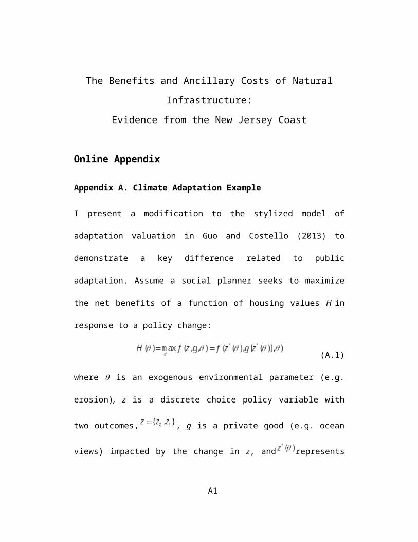
The Benefits and Ancillary Costs of Natural Infrastructure:

Evidence from the New Jersey Coast

Online Appendix

Appendix A. Climate Adaptation Example

I present a modification to the stylized model of adaptation valuation in Guo and

Costello (2013) to demonstrate a key difference related to public adaptation.

Assume a social planner seeks to maximize the net benefits of a function of

housing values H in response to a policy change:

(A.1)

where is an exogenous environmental parameter (e.g. erosion), z is a discrete

choice policy variable with two outcomes, , g is a private good (e.g.

ocean views) impacted by the change in z, and represents the optimal policy

given . I follow Guo and Costello (2013) by assuming the function f is strictly

concave in and g, differentiable in and g and the envelope function H is

continuous and differentiable. A small change in impacts the value of

adaptation directly through the optimal choice of z and indirectly through the

impacts on g resulting from that optimal choice.

(A.2)

A1

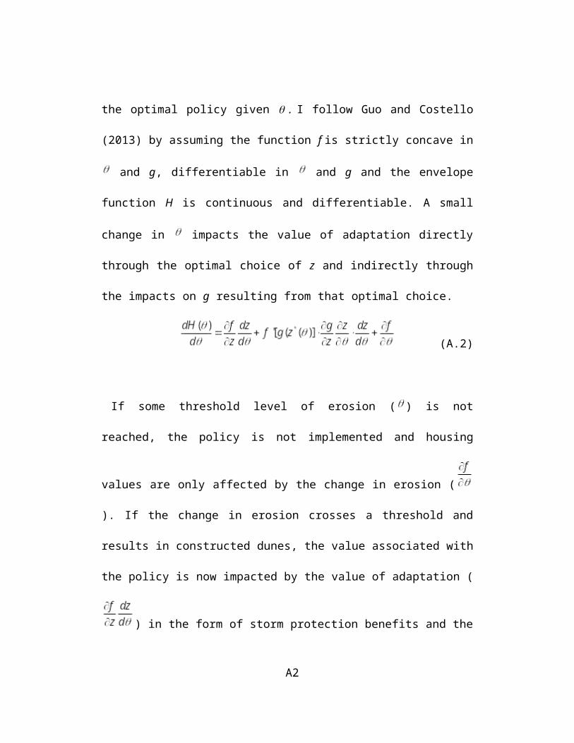
If some threshold level of erosion ( ) is not reached, the policy is not

implemented and housing values are only affected by the change in erosion ( ).

If the change in erosion crosses a threshold and results in constructed dunes, the

value associated with the policy is now impacted by the value of adaptation (

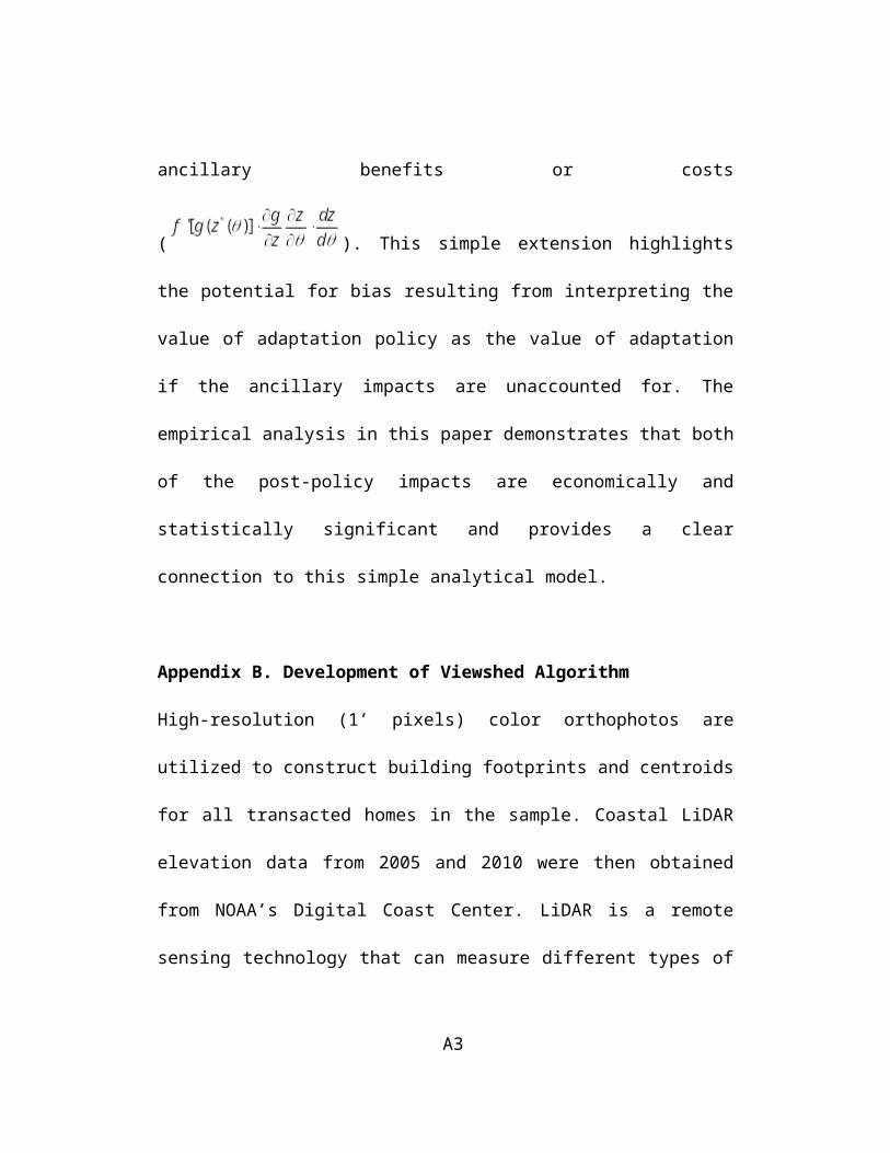
) in the form of storm protection benefits and the ancillary benefits or costs

( ). This simple extension highlights the potential for bias

resulting from interpreting the value of adaptation policy as the value of

adaptation if the ancillary impacts are unaccounted for. The empirical analysis in

this paper demonstrates that both of the post-policy impacts are economically and

statistically significant and provides a clear connection to this simple analytical

model.

Appendix B. Development of Viewshed Algorithm

High-resolution (1’ pixels) color orthophotos are utilized to construct building

footprints and centroids for all transacted homes in the sample. Coastal LiDAR

elevation data from 2005 and 2010 were then obtained from NOAA’s Digital

Coast Center. LiDAR is a remote sensing technology that can measure different

types of elevation by beaming lasers from low-flying aircraft and analyzing the

reflected light. The data provide both baseline and first-returns digital elevation

A2

models (DEM) for Long Beach Island smoothed with an inverse distance

weighting algorithm at 6’ spatial resolution. The baseline DEM depicts the

elevation of the barrier island and the first-returns DEM represents the top of all

buildings and vegetation on the island. The 2005 first-returns LiDAR provides a

pre-dune baseline for the analysis since construction on the first dune did not

begin until September 2006. The most recent LiDAR data available (2010)

contains both the Surf City and the Harvey Cedars dune. The Brant Beach dune,

built in 2012, was incorporated into the 2010 first-returns DEM raster in ArcGIS

using the concept burn streams into DEM to complete the post-dune DEM for

analysis. This process is designed to add decrements in DEMs for streams and

other water features. I simply altered the decay coefficient algorithm to instead

add increments of elevation to the shoreline in Brant Beach where the dune was

eventually constructed. The process can be characterized by the following

equation:

DE = E + (G / (G + D))k × H (B.1)

where DE is the newly calculated elevation representing the dune, E is the old

elevation from the DEM, G is the grid resolution, D is the distance from the dune

peak, k is the decay coefficient, and H is the elevation increment. An appropriate

facsimile of the Brant Beach dune was generated with k = 2 for the decay

coefficient and H = 10 for the average increase in the shoreline height from the

construction of the dune.

A3

An iterative geo-processing algorithm utilizes the data described above to

capture the degree of ocean view from each home. For each parcel in each time

period, the building footprint is zeroed out to the baseline elevation. This step

ensures that the observer “sees” past the confines of the house. Then, an

observation point is defined for both the first (10’) and second floor (20’) of the

house. The tool then determines the amount of the Atlantic Ocean that can be

seen from each observation point across the first-returns DEM, with a maximum

view of 180°. This view is then calculated with the following formula:

View° = ArcLength/π * 180° (B.2)

where ArcLength is the value returned by the tool capturing the arc of a circle in

the ocean that is visible from each observation point. Once both views are

recorded, the algorithm then replaces the building footprint in the first-returns

DEM and moves on to the next parcel.

Figure B.1 provides an example of the algorithm results for first floor view

from an oceanfront parcel in Surf City. The results indicate a nearly 62°

reduction in this view as a result of the dune construction in 2006.

A4

Figure B.1. First Floor Viewshed from a Surf City Oceanfront ParcelNotes: The red dot is the centroid of the housing footprint for the oceanfront parcel. The half circle outlined in black represents extent of possible ocean view from the first floor of that specific parcel. Yellow areas represent the area of the ocean visible to an observer on the first floor of the home. The degree measures of ocean view shown above were calculated as follows: View° = Arc Length/π * 180.

A5

109.1° 47.3°

2010: After the Dune2005: Before the Dune

Appendix C. Additional Figures and Tables

Table C.1: Damage and Federal Aid for Sandy Relief on Long Beach Island

Notes: Surf City, Harvey Cedars received dunes and beach replenishment prior to Sandy. Barnegat Light has a substantial natural dune system and data is provided for comparison purposes Damages are considered minor under $8,000. Damages are considered major between $8,000 and $28,800. Damages are considered severe above $28,800. NFIP does not break down payments by storm, but discussion with local officials confirms a majority of these payments were related to Sandy.

Source: Data in Panels A and B from the NJ Department of Community Affairs. Panel C data from NFIP: http://bsa.nfipstat.fema.gov/reports/1040.htm#34

A6

Long Beach Township

Harvey Cedars Surf City Ship

Bottom Beach Haven Barnegat Light

Panel A. Housing Damages related to SandyHousing Units 8418 1218 2583 2031 2549 1252Homes Damaged 810 64 608 829 260 17Rentals Damaged 198 12 55 110 109 2Percent Impacted 12.0 6.2 25.7 46.2 14.5 1.5Major Impact (%) 8.5 5.0 2.0 4.0 10.2 1.2Severe Impact (%) 2.0 0.7 0.6 2.5 2.2 0.2Panel B. Non-NFIP Federal Funds Distribution for Sandy ReliefTotal Federal Funds $11,088,034 $1,269,886 $2,092,094 $7,364,868 $12,972,642 $549,457

per capita $3,618.81 $2,475.41 $1,689.90 $6,707.53 $10,892.23 $988.23Panel C. National Flood Insurance Data (1/1/78 to 5/31/14)Total Loss Claims 7,519 857 1,381 1,616 2,609 238

Total Payments $214,831,368 $10,188,404 $20,877,434 $61,387,954 $83,761,839 $2,589,196

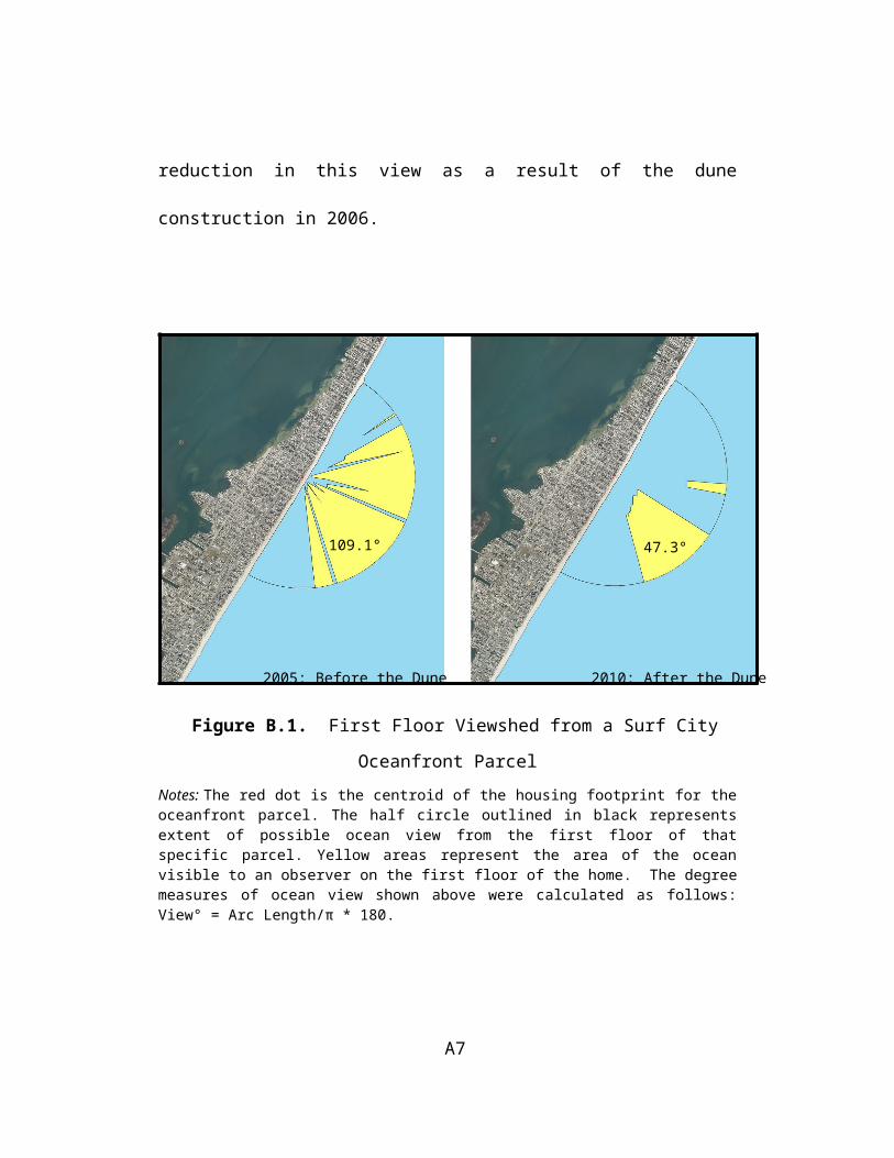
Table C.2: Results of Falsification Tests

Falsification TestFull Model

Falsification TestDID decomposition model

Coefficient Std. Error Coefficient Std. ErrorDune Treatment (OB) -0.013 0.010Dune Treatment (DID) -0.025 0.020

Treated*Dune Area - - -0.0002 0.0003Treated*Lateral Distance (ft) - - -6.08e-06 4.02e-06Treated*Ocean View (°) - - 0.0002 0.0015Treated*Beach Width (ft) - - 0.0003 0.0002

Note: Models are specified in the exact same manner as the preferred models. All treated observations are removed from the analysis. Treatment is falsely assigned to three communities that share a border with the treated communities (Ship Bottom, Loveladies, and Brighton). Both the falsification test with the full OB and DID models and the amenity decomposition DID model do not indicate any statistically significant spillover effects into control communities.

A7

Table C.3: Reference Coefficients for Oaxaca-Blinder Model

Treated Group ( )N= 357

Control Group ( )N=4,470

Reference ( )

Coefficient Std. Error Coefficient Std.

ErrorCoefficient Std.

Error# of Bedrooms 0.048 0.047 0.160*** 0.018 0.152*** 0.018 Rooms2 0.004 0.005 -0.018*** 0.002 -0.017*** 0.002# of Bathrooms 0.077 0.051 0.103*** 0.014 0.103*** 0.014 Baths2 -0.021*** 0.008 -0.007*** 0.002 -0.007*** 0.002Square Footage 0.00005*** 0.036 0.0002*** 0.000 0.0002*** 0.000 SqFeet2 -1.0e-07*** 2.76e-08 -7.6e-09*** 8.3e-10 -7.1e-09*** 9.3e-10Lot Size (sq. ft) 0.033*** 0.002 8.7e-06*** 1.7e-06 8.7e-06*** 1.7e-06 LotSize2 -1.3e-09 1.3e-09 3.7e-10*** 9.1e-11 3.5e-10*** 9.1e-11Age of home -0.009*** 0.002 -0.007*** 0.001 -0.007*** 0.001 Age2 5.9e-05** 2.5e-05 0.000*** 5.9e-06 0.000*** 5.8e-06Oceanfront 0.420** 0.203 0.300*** 0.047 0.309*** 0.047Oceanfront Block 0.424*** 0.105 0.076** 0.030 0.088*** 0.030Second Block 0.068 0.083 0.068*** 0.023 0.061*** 0.023Third Block 0.090* 0.048 0.045*** 0.016 0.045*** 0.016Bayfront 0.332*** 0.073 0.329*** 0.019 0.329*** 0.019Condo -0.304* 0.166 -0.440*** 0.024 -0.449*** 0.023Garage 0.042* 0.024 0.046*** 0.008 0.048*** 0.008Hot Tub 0.113** 0.045 0.029** 0.012 0.030** 0.012Fireplace 0.050* 0.027 0.030*** 0.007 0.035*** 0.007Dist. to Ocean (ft) 0.0003 0.0004 -0.0000*** 0.000 -0.0000*** 0.000Dist. To Bay -0.0003*** 0.0001 -0.0001*** 0.000 -0.0001*** 0.000Dist. to Public Access -0.0002 0.0003 -0.0000 0.000 -0.0000 0.000Dist. to Comm. Distr. 0.0001** 0.0000 0.0002*** 0.000 0.0001*** 0.000Quarter & Year FE Y Y YNeighborhood FE Y Y YFlood Zone FE Y Y YConstant 13.712*** 0.554 12.414*** 0.085 12.468*** 0.084

*** Significant at the 1 percent level. ** Significant at the 5 percent level. * Significant at the 10 percent level

A8

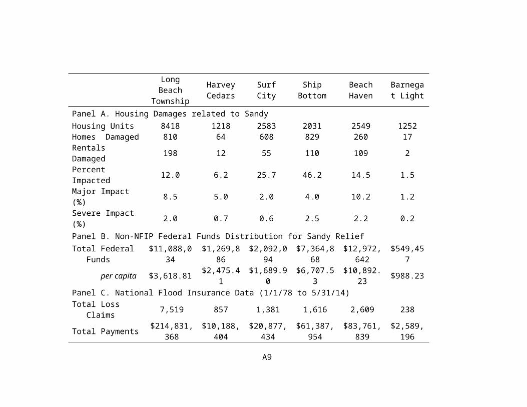
Figure C.1. Transactions Prices in Surf City and Ship Bottom: PCA SigningNotes: Black line is Surf City and grey line is Ship Bottom. The trend lines are estimated separately for the time periods before and after the signing of the Project Cooperation Agreement between USACE and the NJDEP using nonparametric regressions with a tri-cube weighting function and a bandwidth of 0.5. The vertical line represents the date the Project Cooperation Agreement was signed (August 2005).

A9

Figure C.2: Timeline of Important Events Related to Dune Construction on LBI

A10

Sept. 2009

NJDEP sues holdouts in Surf City, paving way for

project to begin

June 16, 2006

Harvey CedarsApproves use of Eminent

Domain on Easement Holdouts

July 15, 2008

Dredging Contract signed for Brant Beach Project

Sept. 30, 2011

Project Cooperation Agreement Signed by

USACE & NJDEP

Aug. 17, 2005

Brant BeachDune Construction

Harvey CedarsDune Construction Post-Tropical Cyclone

SANDY

Surf City Dune Construction

USACE Feasibility Report Issued

June 2012

Mar. 2012

Feb. 2007

October 29, 2012

April 2010

Oct. 2006Sept. 1999

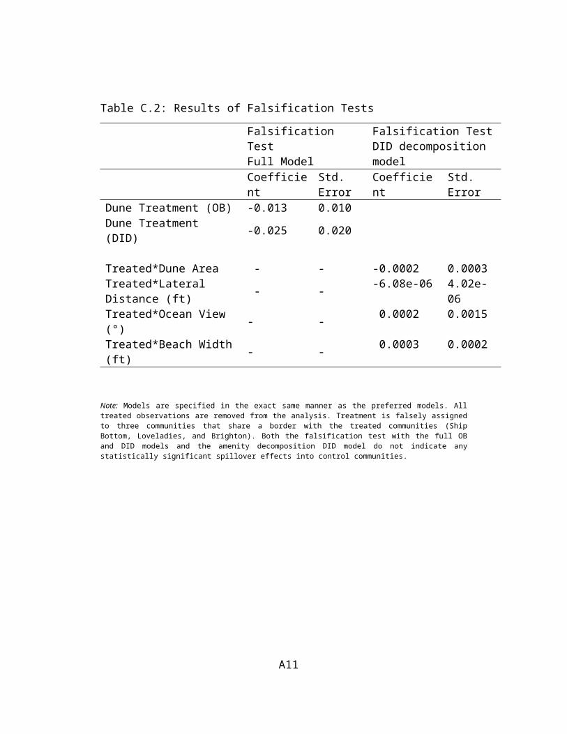
Figure C.3. Price Trends in Brant Beach v. Control CommunitiesNotes: Black dots indicate individual housing transactions by month. Linear price trends for the two primary treated communities compared to all control communities both before and after dune construction activities. Year dates on the horizontal axis indicate the beginning of each year (i.e. 2011 = January 2011, etc.). Shaded areas represent dune construction activities and transactions during this time are removed to avoid any impacts this activity may have on home prices. Dotted lines are added to the shaded area to demonstrate the trend from pre-dune to post-dune periods in each group.

A11