Appendix 4: ecosystem services hypotheses

Snohomish Basin Scenarios Report 2013 Appendix 4: Ecosystem Services Hypotheses A4-1

Appendix 4: ecosystem services hypothesesThe Snohomish Basin supports a multitude of resources and services that are supplied by natural ecosystems. Collectively, these benefits are known as ecosystem services and include products like clean drinking water and processes such as the decomposition of wastes. The Millennium Ecosystem Assessment (MEA) identifies four categories of ecosystem services: provisioning (e.g. food and water), regulating (e.g. carbon sequestration and waste decomposition), supporting (e.g. soil formation and seed dispersal) and cultural (e.g. recreation and inspiration) [1]. Some ecosystem services are already accounted for in our economic system, especially provisioning services. Others, such as regulating and supporting services, have been largely considered “externalities”, assumed to be relatively inexhaustible. However, in our modern, highly populated world with its dramatically altered landscape, many of these ecosystem services have been damaged and reduced [1].

The following pages describe the relevance, current conditions and alternative hypothetical trajectories for ecosystem services including: water quality [A4-2] and quantity [A4-4], carbon stocks [A4-6]and fluxes [A4-8], and habitat [A4-10] and genetirc diversity [A4-12]. Hypothetical future trajectories are predicated on the assumptions relating changes in key drivers to changes in selected ecosystem services. These hypotheses have not been tested through quantifiable models1. The following hypotheses are intended to reflect potential uncertainty around future conditions and important relationships to consider when exploring the use of integrated predictive model to forecast future changes.

A4-2

Water Quality

Why is water quality and stream temperature important: Generally speaking, water quality is important for both human and ecosystem health. Stream temperature is particularly important as it governs the kinds of life that can live in a stream. Fish, insects, and other aquatic species all have a preferred temperature range[2]. The rate of chemical reactions generally increases with higher temperatures, influencing biological activity (e.g. metabolisom) [2]. For example, the amount of dissolved oxygen in stream water is highly dependent on water temperature – hotter water holds less oxygen.

What are past trends and current conditions of stream temperature in the basin?

Dozens of agencies in the Snohomish basin and the Puget Sound Region track stream temperatures including the Department of Ecology, USGS, and King and Snohomish County[3]. Spatial and temporal data allows for comparisons across and within streams and over variable time scales. The Department of Ecology, in compliance with the US Clean Water Act, monitors water quality in Washington Streams and keeps track of waters for which beneficial uses such as drinking, recreation, aquatic habitat and industrial use are impaired [4]. In 2008, ten rivers and creeks [Figure A4.1] were classified as ‘category 5’, violating stream temperature thresholds and requiring an improvement project [5]. In 1998, only 5 of these rivers were classified as category 5 for temperature impairments [4].

What are the three major mechanisms by which stream temperature will change in the basin’s future?

climate change: Both atmospheric temperature and seasonal precipitation variability influence stream temperature [6]. Atmospheric temperature rise can directly influence stream temperature. Climate further influences hydrological shifts through the timing and amount of precipitation, and snowmelt. High

temperatures are especially critical during periods of low flows and drought [6].

impervious surface: Major challenges to temperature in the basin include infiltration rates and surface runoff (in terms of the timing and volumes) resulting from increase in impervious surface. Development, and associated impervious surface, precludes infiltration, increases the runoff rates and reducing the timing [7] of overland flows. As waters runs over hot paved surfaces like driveways, roofs and parking lots, it heats up [8]. The distance to water bodies and alterations to vegetation and soil are also important considerations[9]. Development close to water bodies may rise stream temperatures further due to shorter time the water has to cool during transport [9]. Development over high percolating soils and mature forests with thick duff layers is significantly more detrimental than development over clay or already degraded lands.

riparian (stream) buffers: Streamside vegetation slows down surface flow (runoff), giving it time to cool down. Streamside vegetation also shades the water, reducing summer stream temperatures [10].

Figure A4.1 WRIA 7 303d Impaired Streams


Box A4.1 WRF and Stream Temperature

The Weather Research and Forecasting Model (WRF) has multiple uses and specifications. The CCSM3 and ECHAM5 regional models investigate global climate change at a local scale. Mote and Salathe, 2009 estimated stream temperatures within Washington State utilizing the WRF model with both the A1B and B1 global scenarios report [6, p226]. Stream temperature models predict significant increases in stream temperature for both the A1B and B1 emission scenarios. Summertime temperature greater than 18degC will become the norm for Western Washington by the 2040’s and stream temperatures in high elevations of the Cascades will resemble lowland stream temperatures of the 1980’s. By the 2080’s under the A1B scenario the majority of the Snohomish Basin is estimated to be fatal for salmon. Stream temperatures estimated by WRF do not take into account increases due to increased urbanization (e.g. runoff over asphalt) and vegetation removal along stream channels.

Table A4.1 Hypotheses of future trajectory shifts of drivers influencing water quality mechanismsAccelerate small resistance metamorphosis

Water Quality over time

Stream Temperature Hot Cool Very Hot Warm

climate change Minor Minor Major Major

impervious surface Triple Minor Double Increase

riparian Buffers Narrowed Managed Hardened Restored

Figure A4.2 NOAA Advanced Hydrological Prediction Service, River Observations

A4-4

Water QuantityWhy is water quantity and fluctuations in-stream flows important? Water quantity is important because both too little (drought) and too much (flood) can have detrimental impacts on ecosystems and humans. Seasonal variation in stream flow is natural and expected. When the magnitude and frequency of variability exceeds historical trends, it poses a significant challenge. Flood trends are unique per stream, depending on geomorphology (e.g. channel elevation), levels of urbanization, and precipitation timing. Flooding affects urban development in terms of infrastructure (roads and utilities) and properties, incurring costly damages and disruption of services. Flooding in agricultural lands leads to damaged crops, livestock, and built structures. Aquatic wildlife and vegetation can also be affected by floods, as floods carry warmer temperatures and higher levels of pollutants [11]. Floods can also increase sediment loads and disrupt streamside habitat. Alternatively, not enough water can be dangerous and costly. In-stream flow are restrictions specifying the amount of water needed meet future water management objectives for the health of ecosystems and people.

What are past trends and current conditions of streamflow fluctuations in the basin? The Snohomish Basin has abundant water resources [12]. Enough to support over 1 million residents’ drinking water needs, as well as industry cooling, agricultural irrigation, and hydropower, with plenty left over for aquatic life [13]. The challenge lies in the timing of flows, and the low precipitation volumes in the summer [6]. Most of the basin’s precipitation arrives in the winter, when demands are lowest while in the summer, the snowpack is gone and there is little rain, so flows are dependent on groundwater inflow[12]. Traditionally this natural variability has translated into flooding in the winter and spring, and low in-stream flows in the summer. Urbanization has increased the rate of flow in the winter, exacerbating floods, while demands in summer, exacerbate low flows. Historically, King and Snohomish County have the highest cost impacts from floods in the State [14]. Still, several basin streams have moderated levels due to dams and levees that restrict flows.

NOAA monitors stream flow over time [15], as do the Counties [16] and USGS [17]. Comparing several basin gages (Figure A4.3), all seven gages reflect increasing frequencies of peak flows and major floods [15]. The

USGS has reported four stream channels with low flow values below minimums in the basin.

What are the three major mechanisms by which in-stream flows will change in the basin’s future?

Withdrawals: The amount of water that is pulled from the stream, both directly and indirectly (i.e. from aquifers that are the water source for the streams). Water rights govern the amount of water that can be removed from a stream by municipalities, service providers and wells serving more than 6 households. In-stream flows restrict the amount of water that can be withdrawn from a water body, as specified per channel for a defined time and typically follows seasonal variations [18]. The greater the population and industry, the greater the demand and pressure to increase withdrawals [15]. In terms of demand, most of the water in the watershed has already been allocated, and obtaining new water rights will continue to be very difficult [18]. However, indirect withdrawals such as exempt wells and groundwater taps as well as Tribal water use are not restricted by water rights [19]. Further, agricultural irrigation is not forecasted by municipality service provision plans and is largely unmonitored [13]. Water conservation efforts, from high efficiency plumbing and appliances and education, can reduce per capita demand (and has over the last 50 years)[13]2. The Central Puget Sound supports estimated utility goals of additional 12% reductions due to conservation over the next fifty years [13]. As of March 2011, there are 109 pending water right applications for WRIA 7 [18].

climate change: Despite uncertainty in long-term precipitation trends, it is not forecasted that the annual precipitation will change dramatically over the next fifty years [6]. However, the timing of precipitation and snowmelt will have significant impacts on streamflow fluctuations [6, 13]. As described under the snowpack and streamflow section, the basin is forecasted to eventually eliminate springtime snowmelt and reduce summer in stream flows.

impervious surface: The urban hydrograph, dominated by impervious surfaces, is marked by higher and faster peaks [20]. Already the Snohomish, Raging and Tolt are characterized by shifted streamflows associated with urbanization [21]. Further urbanization may lead to exceeded thresholds with markedly low summer flows and flush floods in the winter [20].


Box A4.2 DHSVM and Stream flow:

The distributed hydrology-soil-vegetation model (DHSVM) is a regional-scale model forecasting hydrologic components and flood statistics based on meteorological records and land surface characteristics. The models has recently parameterized at the University of Washington to assess impacts on the hydrology of Puget Sound by urbanization and climate change. Cuo et al explored the effects of forecasted land cover change (LCCM) and climate change on streamflows in the Puget Sound by 2050[52]. While climate impacts largely control the seasonal variability of streamflow, urbanization increases runoff year-round. The eastern lowlands are expected to experience the greatest effects of urbanization, and hence the greatest hydrologic changes; this region is more sensitive to these effects than to climate change. The combined effects of climate and land cover change on the seasonal distribution of streamflow is 12-42% increase flow in the winter and 15-40% decrease flows in late spring and summer. Snohomish Basin specific estimations coupling climate and land cover change have not been estimated at the time of this writing. The DHSVM model has not been explored in conjunction with alternative withdrawal estimates not with the potential variability associated in the Snohomish Basin Scenarios.

Figure A4.3 Streamflow variability 1960-2010.

Table A4.2 Hypotheses of future trajectory shifts of drivers influencing water quantity mechanisms

Accelerate small resistance metamorphosis

Water Quantity over time

In Stream flows Dirty and drawn (urbanization increases drinking water demand and overland flows flush through the paved system)

Cycled and stable (resource managers cycle use, treatment and release on-site)

Fast and early (Early snowmelt coupled with sprawls and levees exacerbates flow variability)

Variable but buffered (extreme climate events are buffered by riparian areas and efficient withdrawals)

Withdrawals Major demand Local Resource Deep Drills Moderated

climate change Minor Minor Major Major

Urbanization Triple Minor Double Increase, buffered

A4-6

carbon stocks

the carbon cycle: The impact of urbanizing watersheds on the global carbon cycle has started to generate new evidence of the complex mechanisms linking urbanization to carbon emissions and uptake [22]. The net carbon balance of terrestrial ecosystems is typically assessed as the difference between gross primary production (GPP) and respiration (R). Urbanization directly and indirectly affects carbon stocks (pools of carbon such as plants) and carbon fluxes (e.g, emissions of CO2). Urbanization increases impervious surface area, which alters the hydrology and reduces infiltration capacity and the microclimate. Urban activities add multiple pollution sources, including chemical inputs from industry, agriculture, and transportation. Finally, land-cover changes typically result in changes in plant species and size composition, affecting rates of C assimilation. The mechanisms influencing C stocks (pools of C) are distinct from those influencing C fluxes (rates of exchange).

Why are carbon stocks important? Why forest biomass? [23]Forests store large quantities of carbon within their live and dead organic material. Human and naturally caused disturbances to forests can shift these stocks quickly into the atmosphere; increasing CO2 concentrations. Carbon uptake by urban forests can significantly reduce local emissions and atmospheric CO2 concentrations. While carbon emissions, from vehicles, industry and residences are a critical component of the urban carbon cycle, they are not the entire budget. Characterization of carbon stocks and fluxes in urban forests is critical to understanding if an area is a net carbon sink or source. Baseline accounts of carbon stocks in urbanizing areas are very important, but can be challenging as land cover and vegetation are constantly changing. Carbon stocks vary greatly by region and condition. For example, Smithwick [24] found that old forests in the Western Cascades of Washington can store near 450 Mg C per hectare. However, recovering and or younger forests can uptake more carbon while storing lower carbon stocks.

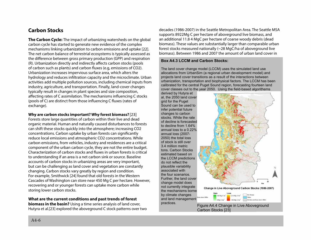
What are the current conditions and past trends of forest biomass in the basin? Using a time series analysis of land cover, Hutyra et al.[23] explored the aboveground C stock patterns over two

decades (1986-2007) in the Seattle Metropolitan Area. The Seattle MSA supports 8922Mg C per hectare of aboveground live biomass, and an additional 11.8 4 MgC per hectare of coarse woody debris (dead biomass). These values are substantially larger than comparable urban forest stocks measured nationally (~28 MgC/ha of aboveground live biomass). Between 1986 and 2007 the amount of urban land cover in

Box A4.3 LCCM and Carbon Stocks:

The land cover change model (LCCM) uses the simulated land use allocations from UrbanSim (a regional urban development model) and projects land cover transitions as a result of the interactions between urbanization, transportation and biophysical factors. The LCCM has been calibrated for the central Puget Sound region, forecasting fourteen land cover classes out to the year 2050. Using the field-based algorithems derived by Hutyra et al, the 2050 land cover grid for the Puget Sound can be used to infer potential future changes to carbon stocks. While the rate of decline is forecasted to decline from 1.64% annual loss to a 0.22% annual loss (2007-2050) the total loss of stock is still over 3.4 million metric tons. Carbon Stocks estimated based on the LCCM predictions do not reflect the plausible variability associated with the four scenarios. Further, the land cover change model does not currently integrate the mechanisms borne by climate changes and land management practices.

Figure A4.4 Change in Live Aboveground Carbon Stocks [23]


the basin doubled, virtually all at the expense of forests. Hutyra et al. estimate that during the same time frame, aboveground carbon stocks were lost at a rate of 1.2Mg C per hectare per year. The majority of the carbon losses occurred at the rural fringe, a distance greater than 7.5km (4.5 miles) from the Seattle city center as within the urban area there was little available forest land cover for development. Carbon stocks and losses within Snohomish Basin are even more dramatic. Rough estimates show average densities of 155MgC/ha in WRIA 7 in 2007 (as compared to 100Mg in the Seattle MSA). With a total aboveground terrestrial carbon stock of over 56 million MgC – The basin supports more aboveground carbon than WRIAs 8, 9 and 10 combined (the remainder of the Seattle MSA).

What are the three major mechanisms by which forest biomass will change in the basin’s future?

Urban development: Higher rates of forest conversion associated with urbanization result in a reduction of terrestrial C stocks [44]. Average aboveground carbon stocks vary greatly depending on the nature of development – from high urban areas with carbon densities of 2Mg/ha to coniferous forests supporting over 183 Mg/ha. Carbon stocks at the urban fringe are likely the most susceptible due to high densities and high rates of conversion.

Table A4.3 Hypotheses of future trajectory shifts of drivers influencing carbon stocks mechanismsAccelerate small resistance metamorphosis

Carbon Stocks over time

Forest Biomass Rapid loss reaches critical limits

Minor loss stabilized Continual gradual loss Initial loss rebounds

Urban development 20% forest cover loss mostly in lowlands

2010 levels maintained 15% forest cover loss – high at rural fringe

5% forest cover loss – mostly in lowlands

Land management Intense rotations and extractions

Sustainably managed Cleared and manipulated Diverse and native

Biogeochemical cycles Heavy inputs Moderate inputs Inputs and climate altered cycle

Minimal inputs, altered cycle

Land management: Resource management, whether by timber companies, by park maintenance or by households, can influence tree removal, tree species selection and understory clearings. For example, shorter rotation cycles and understory clearing lead to lower carbon stocks in forests. Urban land-use and management practices affect soil organic matter directly by removing the mass and nutrients from leaf and woody debris [45]. These organic carbon stocks are kept artificially low in urban and suburban areas through yard maintenance practices, but the carbon fluxes (input rates) would be expected to increase linearly across the urban to rural gradient (directly proportional to biomass/leaf area index).

Biogeochemical cycles: human modifications of nutrients including nitrogen, phosphorus and carbon, at a global scale influence plant growth rates. For example, nitrogen is historically a limiting factor in tree growth, but substantial nitrogen inputs to ecosystems by global agricultural and household fertilization practices has shifted growth curves. Different plants, from invasives to native Douglas firs, respond differently to altered cycles. Both N and CO2 fertilization have been associated with an increase in C uptake. N fertilization has been found to occur in temperate ecosystems that are currently nitrogen limited [26]. Increasing N inputs (via pollution and fertilization) will, over long time periods, result in enhanced C stocks. The responses of ecosystems to CO2 fertilization are limited by the availability of N in the system.

A4-8

carbon Fluxes

What are carbon fluxes and carbon emissions important? C fluxes are exchanges between two different stocks, such as the transfer of CO2 from the atmosphere to the biosphere via plant photosynthesis, or emissions of CO2 to the atmosphere from combustion processes. Emissions, from cars, industry and homes are one form of fluxes, while decomposition of organic matter also produces CO2. Urban and urbanizing areas are a major source for emissions of CO2 with estimates of 90% of all emissions directly or indirectly attributed to urban areas [27]. CO2 is a powerful greenhouse gas – meaning that it traps heat within the earth’s atmosphere, contributing to global warming.

What are past trends and current conditions of carbon fluxes in the basin? King and Snohomish County’s per capita emissions are were estimated at 2.83 and 2.4 Mg C per year (2002, respectively). The majority of the emissions stemmed from ‘on-road’ sector including cars, trucks and buses (52% in Snohomish and 49% in King). Residential, industrial and aircraft emissions accounted for the majority of remaining fluxes. On average, the EPA estimates that for every vehicle miles traveled (VMT) 423g of CO2 are emitted [28]. Between 2008 and 2009, drivers in King and Snohomish Counties cumulatively drove over 21 billion miles [29], potentially emitting over 248 million Mg C. The number of vehicles miles travelled in the region has more than doubled since 1980 [29]. Meanwhile, the fuel efficiency has reduced national vehicle emissions per mile traveled by ~1.17% a year [30].

What are the three major mechanisms by which carbon emissions will change in the basin’s future?

Urban development: Urban development affects the carbon cycle through both direct and indirect pathways, with increasing fossil fuel emissions among the most significant of such impacts [22]. Forty percent of total fossil fuel emissions in the United States are attributed to the transportation and residential sectors [31]. Factors that likely affect per capita CO2 emissions include

population and housing densities, the rate of population growth, affluence, and technologies [32]. Demographic trends together with increase produce an overall increase in per capita CO2 emissions and an increase in the consumption of land associated with urban development. The pattern of urban development may be key to determining the extent to which urbanization will contribute to CO2 emissions, since the spatial distribution of residential and commercial housing units affects commuting patterns and transportation choices. Future trajectories of urban form and infrastructure choices will be decisive in future CO2 emissions. At the same time, as a result of land-use and management practices which affect mass and nutrients from leaf and woody debris removal, C sequestration would be expected to decrease directly proportional to loss of biomass/LAI [33]).

regulations and innovations: Efficiency refers to the level of emissions per mile driven or watts consumed. Regulations, such as the EPA’s CAFE standards govern the level of allowable efficiencies. Innovative technologies providing cost-effective and reliable substitutes can further drive higher efficiencies.

climate change: As the temperature rises, biogeochemical cycles quicken, releasing more atmospheric carbon through respiration and decomposition. Soil respiration rates could be expected to increase with increasing urban temperatures. Urban heat islands also affect soil respiration rates, which are expected to be higher within the urban interior due to exponential relationship between respiration and temperature. Given the simultaneously changing N inputs and atmospheric CO2 concentration across the urban gradient, we would also expect the CO2-fertilization effects to affect carbon fluxes by changes in N inputs and CO2 concentrations/emissions.


Box A4.4 UrbanSim and Carbon Emissions:

UrbanSim is a parcel based land use model. It allocates land use (location of households, employment and population) given inputs of current development patterns, restrictions, transportation, and regional economic forecasts. Currently, The Puget Sound Regional Council (PSRC) operates UrbanSim within the Central Puget Sound area out to 2040. UrbanSim works in concert with PSRC’s Travel Demand Forecast which generates estimates vehicle miles traveled. Forecasted vehicle emissions can be quantified based on estimated vehicle miles traveled in the Basin. Based on rough initial estimates, the basin will see an additional 4,407,000 VMT per weekday by 2040 (a 40% increase on the current 10,980,000 VMTs, and an approximately additional 1,820 metric tons of C02 emitted per day [53]). By exploring alternative urban development and transportation scenarios decision makers can forecast alternative emission outcomes. Estimations of carbon emissions based on UrbanSim’s VMT transportation output do not integrate the mechanisms borne by new regulations, innovations or climate changes.

Figure A4.5 Travel Model Forecasted VMTs for Basin 2040.

Table A4.4 Hypotheses of future trajectory shifts of drivers influencing carbon emissionsAccelerate small resistance metamorphosis

Carbon emissions over time

Carbon emissions Increase Stabilize Exponential growth Decline

Urban development Extensive Minor but rural Sprawled Urbanregulations and innovations

Rapid private market innovations

Regulations increase Stagnate, deprioritized Global, integrated

climate change Minor temperature rise Minor temperature rise Major temperature rise Major temperature rise

A4-10

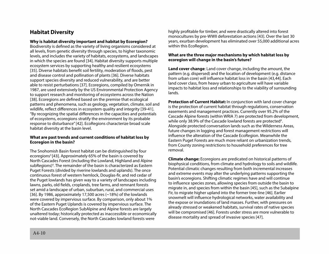
habitat diversityWhy is habitat diversity important and habitat by ecoregion? Biodiversity is defined as the variety of living organisms considered at all levels, from genetic diversity through species, to higher taxonomic levels, and includes the variety of habitats, ecosystems, and landscapes in which the species are found [34]. Habitat diversity supports multiple ecosystem services by supporting healthy and resilient ecosystems [35]. Diverse habitats benefit soil fertility, moderation of floods, pest and disease control and pollination of plants [36]. Diverse habitats support species diversity and reduced vulnerability, and are better able to resist perturbations [37]. Ecoregions, compiled by Omernik in 1987, are used extensively by the US Environmental Protection Agency to support research and monitoring of ecosystems across the Nation [38]. Ecoregions are defined based on the premise that ecological patterns and phenomena, such as geology, vegetation, climate, soil and wildlife, reflect differences in ecosystem quality and integrity [39-41]. “By recognizing the spatial differences in the capacities and potentials of ecosystems, ecoregions stratify the environment by its probable response to disturbance” [42]. EcoRegions characterize broad scale habitat diversity at the basin level.

What are past trends and current conditions of habitat loss by ecoregion in the basin?

The Snohomish Basin forest habitat can be distinguished by four ecoregions3 [43]. Approximately 65% of the basin is covered by North Cascades Forest (including the Lowland, Highland and Alpine subRegions)4. The remainder of the basin is characterized as Eastern Puget Forests (divided by riverine lowlands and uplands). The once continuous forest of western hemlock, Douglas-fir, and red cedar of the Puget lowlands has given way to a variety of landscapes including lawns, parks, old fields, croplands, tree farms, and remnant forests set amid a landscape of urban, suburban, rural, and commercial uses [36]. By 1986, approximately 17,500 acres (~18%) of the lowlands were covered by impervious surface. By comparison, only about 1% of the Eastern Puget Uplands is covered by impervious surface. The North Cascades EcoRegion SubAlpine and Alpine forests are largely unaltered today; historically protected as inaccessible or economically not-viable land. Conversely, the North Cascades lowland forests were

highly profitable for timber, and were drastically altered into forest monocultures by pre-WWII deforestation actions [43]. Over the last 30 years, exurban development has eliminated over 55,000 additional acres within this EcoRegion.

What are the three major mechanisms by which habitat loss by ecoregion will change in the basin’s future?

Land cover change: Land cover change, including the amount, the pattern (e.g. dispersed) and the location of development (e.g. distance from urban core) will influence habitat loss in the basin [43,44]. Each land cover class, from heavy urban to agriculture will have variable impacts to habitat loss and relationships to the viability of surrounding lands.

protection of current habitat: In conjunction with land cover change is the protection of current habitat through regulations, conservation easements and management practices. Currently over 95.2% of the Cascade Alpine forests (within WRIA 7) are protected from development, while only 38.9% of the Cascade lowland forests are protected4. Alongside protected conversation lands such as the Wilderness Areas, future changes in logging and forest management restrictions will influence the alteration of the Cascade EcoRegion. Meanwhile the Eastern Puget Forests are much more reliant on urbanization trends, from County zoning restrictions to household preferences for tree removal.

climate change: Ecoregions are predicated on historical patterns of biophysical conditions, from climate and hydrology to soils and wildlife. Potential climatic changes resulting from both incremental increases and extreme events may alter the underlying patterns supporting the basin’s ecoregions. Shifting climatic regimes have and will continue to influence species zones, allowing species from outside the basin to migrate in, and species from within the basin [45], such as the Subalpine Fir, to migrate higher upland into the former tree-line [46]. Earlier snowmelt will influence hydrological networks, water availability and the expose or inundations of land masses. Further, with pressures on already stressed or weakened habitats, survival rates of native species will be compromised [46]. Forests under stress are more vulnerable to disease mortality and spread of invasive species [47].


Box A4.5 Potential Vegetation Model and Habitat Diversity:

The Potential Vegetation zone model is developed by the US Forest Service. The model stratifies the landscape into succession and growth potential vegetation zones based on climate and topographic data. The Snohomish Basin is represented by five plant association groups: Western hemlock zone, silver fir and western hemlock zone, mountain hemlock and silver fir zone, subalpine zone and the alpine zone. Precipitation at sea level is the most important determinant of the boundaries between potential vegetation models, explaining 50% of the variation alone. Habitat conversion associated with climate changes could be forecasted by recalibrating the model to future precipitation variability. Potential vegetation maps could be integrated with forecasts of additional mechanisms including land cover change and habitat protections to explore future conversions.

Table A4.5 Hypotheses of future trajectory shifts of drivers influencing habitat loss

Figure A4.6 Ecoregions of the Snohomish Basin

Accelerate small resistance metamorphosisHabitat diversity over time

Habitat loss Nearly all unprotected forests gone by 2040.

By 2060 about 30% of unprotected forests are gone.

By 2060 nearly all protected and unprotected forests are eliminated.

Initial decline due to development. By 2040 all remaining forests are protected. Over time total area increases.

Land cover change Extensive, lowland Minor, dispersed Sprawling upland Dense urban

protection of habitat Minor increase in protections Minor increase in protections Decline in protected lands. Highest protectionclimate change Minor Minor Major Major

A4-12

Genetic diversity

Why is genetic diversity important? Why coho and Chinook?

Genetic diversity refers to the total number of genetic characteristics in the genetic makeup of a species. Genetic diversity is important in preserving unique genetic blueprints that may reduce vulnerability, the support human health, and cultural values, as well as intrinsic values. Within the Puget Sound, salmon have been identified as an important indicator of species diversity. Their historical cultural values, their relationship to ecosystems and food webs, and their sensitivity to alterations of natural habitat through their diverse geographic ranges make them an appropriate benchmark indicator. Within the Snohomish Basin, twelve wild stocks are currently present, in various relative conditions. The Snohomish Basin Technical Committee identified Chinook salmon (Onchorhynchus tshawytsha), bull trout (Salvinus confluentus) and coho salmon (Onchorhynchus kistuch) as proxy species to represent all anadromous salmonids the in basin for their assessment [48]. Coho and Chinook appropriately represent salmonids needs as they require diverse habitat and occupy the full geographic range of anadromous habitat in the basin [48].

What are past trends and current conditions of chinook and coho in the basin? [48]

The Snohomish Basin is one of the primary producers of anadromous salmonids in the Puget Sound. However, current production is estimated to have substantially declined from historical levels [48].

chinook salmon naturally spawns in the basin and is divided by Skykomish and Snoqualmie populations. Historic equilibrium abundance for the Skykomish and Snoqualmie Chinook populations are 51,000 and 31,000 fish, respectively. Basin managers’ data show that between 1999 and 2003, the average Chinook escapement for the basin was 3,5316, around 5.7% of the historic equilibrium abundance7.

coho salmon in the Puget Sound are designated as species of concern under the Endangered Species Act, which means that concerns exist about certain risk factors, such as population decline and loss of habitat. Coho salmon are relatively abundant in the Snohomish River basin as

compared with other basins in the Region. Four Coho stocks reside in the basin. While survey data for spawning exists, it is difficult to monitor abundance, and the extent of historical Coho range is much greater than the one being monitored today.

What are the three major mechanisms by which salmon viability will change in the basin’s future?

Habitat loss and degradation have been the primary causes of salmon species loss [49]. Identifying mechanistic linkages between land use change and salmon populations is critical to forecasting future population viability.

stream alterations8: Direct alterations to salmon habitat and migration, including barriers such as dams and culverts and shoreline hardening from levees and docks.

Urban and agricultural runoff9: Indirect alterations to water quality, including pollutants and nutrients carried with surface runoff over impervious surfaces and fertilized fields. Reduced water quality impacts salmon survival through toxicity and competition from nutrient-sensitive vegetation and forage fish. The EPA and Department of Ecology monitor water quality of basin streams in terms of turbidity, dissolved oxygen, pH, nitrogen and phosphorus concentration, temperature, metals and organics. While urbanization is likely to continue to increase in the future, strict regulations for non-point source pollution and greater stream buffers may reduce pollution.

streamflow Fluctuations: Streamflow variability is dependent on infiltration (land cover change), inputs (as influenced by climatic impacts to hydrology in terms of snowpack) and withdrawals (the amount of water we take out of streams as influenced by demands, regulations and conservation). While floods, in general, do not negatively impact salmon, they can be disastrous when coupled with high temperatures, turbidity, and lack of channel complexity through vegetation and pools [50]. On the other extreme, droughts and very low flows can harm salmon not only by restricting migration, but as also because low volumes concentrate poor water quality conditions [51].

notes


Box A4.6 SHIRAZ and Salmon Viability [50]:

The Salmon Habitat Integrated Resource Analysis Zowie! (SHIRAZ) is a fish population model. It translates the effects of changes in habitat conditions resulting from land use (development, restoration, hydropower, etc) and climate change into consequences for salmon population status and likelihood of recovery. The Shiraz model provides estimates of four important criteria for describing viable salmon populations (VSP): abundance, productivity, spatial structure, and diversity. Local applications include joint work between NOAA and the University of Washington to assess the influence of climate change (Battin et al 2007) and land use scenarios (Scheuerell et al 2006) on the Chinook salmon population in the Snohomish River Basin. Exploring the variability of downscaled climate projections and a ‘bunsiness as usual’ versus a ‘restoration’ land use scenario, SHIRAZ estimated between a 4.6 – 38% loss in mean returning Chinook spawners between 2000 and 2050. While the SHIRAZ forecast did take into account both streamflow fluctuations associated with land cover and climate changes and stream alterations, it did not manipulate variability in toxins associated with runoff. The SHIRAZ land development models do not reflect the variability of the Snohomish Basin Scenarios.

Figure A4.7 Change in Mean Returning Chinook Spawners, 2000-2050

Table A4.6 Hypotheses of future trajectory shifts of drivers influencing salmon viabilityAccelerate small resistance metamorphosis

Species diversity over time

(chinook = solid and coho = dashed)

Salmon viability Chinook and Coho severely declining.

Coho improved Extinct. Chinook Improved. Coho declining.

stream alterations (hardening)

Urbanized streams, narrowed buffers

Restoration and hardening – channel specific

Significant alterations Wide natural buffers

runoff (toxicity) Novel toxins Rural toxins High toxicity Regulated and minimized

streamflow fluctuations (in stream flows)

Very low infiltration rates) Channel specific withdrawal challenges

Extreme fluctuations - major climatic changes and low infiltration rates

Highly variable - early snowmelt and extreme precipitation events)

A4-14

1. The Integrated Model Workshop, held November 2011, developed a draft blueprint for how models could assess specific indicators of ecosystem services including stream variability in terms of frequency and intensity of peak and drought levels (measuring water quantity), available snowpack, fecal coliform, pesticides, water temperature (measuring water quality), salmon escapement per species (measuring species diversity), mean forest patch size, distribution and extent of land cover, contagion and aggregation index for habitat connectivity (measuring habitat diversity), vehicle miles drivers (measuring carbon fluxes) and acres of forestland along the urban-rural gradient (measuring carbon stocks).

2. Water consumption in Seattle, Tacoma and Everett is less today than it was 40 years ago.

3. Terrestrial ecosystems in the state have been grouped by similar flora, fauna, geology, hydrology, and landforms into nine ecoregions. The delineation of these ecoregions was developed by The Nature Conservancy and many partners on the basis of work done by Robert G. Bailey (U.S. Forest Service), James Omernik (U.S. Environmental Protection Agency), and other scholars.

4. GIS analysis based on 2007 impervious surface and Washington Department of Natural resource State of Washington Natural Heritage Plan’s Ecoregion map.

5. GIS analysis by intersection EPA’s ecoregion clipped to WRIA 7 boundary with a protected lands layers (created by the Urban Ecology Research Lab, including Wilderness lands and administratively withdrawn owl habitat, Mt Hemlock Zone, Mt Goat Habitat, riparian reserves, water, municipal watersheds, foreground (important viewsheds), late successional reserves, late successional and old growth reserves, deer and elk habitat, wildlife habitat, FS land acquired after completion of forest plan, transfer of development rights lands and purchased development land.

6. Escapement refers to number of fish returning to spawn. 3,531 includes 1,755 for the Skykomish and 1,776 for the Snoqualmie population.

7. Equilibrium abundance means that spawning salmon have maximized their use of available habitat and are simply replacing themselves in the next generation.

8. Stream alterations combine artificial barriers and changes to edge habitat.

9. Runoff includes changes in land cover (impervious cover, forest and riparian cover) as well as road density.


references cited1. Millennium Ecosystem Assessment, 2003. Chapter 1: Conceptual

Framework. Island Press. http://www.maweb.org/documents/document.765.aspx.pdf

2. Michaed, J. 1991. A Citizen’s guide to understanding and monitoring lakes and streams. Chapter 3: Streams. http://www.ecy.wa.gov/programs/wq/plants/management/joysmanual/streams.html Last Accessed 04.20.12

3. WA State Department of Ecology (WA DOE), River and Stream Water Quality Monitoring; USGS Water Data for the Nation; King County Land and Water Division; Snohomish County Surface Water Management Division. NOAA Advanced Hydrological Prediction Service, River Observations

4. WA DOE, Washington State’s Water Quality Assessment and 303(d) List; 2008 EPA-approved assessment and 303(d) list. Category 5 refers to Polluted waters that require a TMDL, or the traditional list of impaired water bodies known as the 303(d) list. TMDL is a calculation of total maximum daily load, or amount of pollutant, that a waterbody can receive and still meet water quality standards. Placement in category 5 means that Ecology (WA DOE) has data showing that the water quality standards have been violated for one or more pollutants, and there is no TMDL or pollution control plan. TMDLs are required for the water bodies in this category.

5. Including all freshwater bodies within WRIA 7 classified as category 5 in 2008.

6. Littell, J.S., M. McGuire Elsner, L.C. Whitely Binder, and A.K. Snover (eds). 2009. The Washington Climate Change Impacts Assessment (WCCIA): Evaluating Washington’s Future in a Changing Climate - Executive Summary. In The Washington Climate Change Impacts Assessment: Evaluating Washington’s Future in a Changing Climate, Climate Impacts Group, University of Washington, Seattle, Washington. Available at: www.cses.washington.edu/db/pdf/wacciaexecsummary638.pdf

7. Environmental Protection Agency. EPA 841-F-03-003. February 2003. Urban Non-point Source Factsheet. http://water.epa.gov/polwaste/nps/urban_facts.cfm

8. Tang, Z. X., Engel, B. A., Lim, K. J., Pijanowski, B. C., & Harbor, J. (2005). Minimizing the impact of urbanization on long term runoff. Journal of the American Water Resources Association, 41(6), 1347-1359.

9. Alberti, M., Booth, D., Hill, K., Avolio, C., Coburn, B., Coe, S., and D. Spirandelli 2007. The impact of urban patterns on aquatic ecosystems: An empirical analysis in Puget lowland subbasins. Landscape and Urban Planning, 80: 345–361.

10. Shandas, V and M. Alberti. 2009. Exploring the role of vegetation fragmentation on aquatic conditions: Linking upland with riparian areas in Puget Sound lowland streams. Landscape and Urban Planning 90: 66-75.

11. Mark D. Scheuerell, Ray Hilborn, Mary H. Ruckelshaus, Krista K. Bartz, Kerry M. Lagueux, Andrew D. Haas, and Kit Rawson. 2006. The Shiraz model: a tool for incorporating anthropogenic effects and fish–habitat relationships in conservation planning

12. WA DOE 1995. Snohomish River Watershed Initial Assessment. http://www.ecy.wa.gov/pubs/95154.pdf

13. Water Supply Forum. 2009. Regional Water Supply Outlook. http://www.watersupplyforum.org/home/outlook/. Last Accessed March 2013.

14. Washington Military Department: Emergency Management Division. 2004. Washington State Hazard Mitigation Plan. Hazard Profile: Flood. http://liveweb.archive.org/http://www.emd.wa.gov/plans/documents/Tab_7.1.4_Flood_final.pdf

15. NOAA Northwest River Forecast Center: River Information and Forecasts. http://www.nwrfc.noaa.gov/rfc/

16. King County Flooding Services. Flood Warning and Alerts. http://www.kingcounty.gov/environment/waterandland/flooding/warning-system.aspx; Snohomish County Real Time Flood Warning Information. http://www.co.snohomish.wa.us/PWApp/SWM/floodwarn/index.html

A4-16

17. USGS Water Resources. 2012. National Water Information System: Web Interface. http://waterdata.usgs.gov/nwis

18. WA DOE, 2011. Focus on Water Availability: Water Resource Program. Snohomish River Watershed, WRIA 7. August 2011. http://www.ecy.wa.gov/pubs/1111012.pdf

19. Interview with Water and Energy Group, 2010.

20. Paul, M.J. and Meyer, J.L. 2001. Streams in the Urban Landscape. Annu. Rev. Ecol. 32:333-65.

21. King County Flood Control District. Snoqualmie / South Fork Skykomish River Basin. http://www.kingcountyfloodcontrol.org/default.aspx?ID=45

22. Pataki DE, Carreiro MM, Cherrier J, Grulke NE, Jenning V, Pincetl S, Pouyat RV, Whitlow TH, Zipperer WC. 2011. Coupling biogeochemical cycles in urban environments: Ecosystem services, green solutions, and misconceptions. Frontiers in Ecology and the Environment 9: 27-36.

23. Hutyra, L.R., Yoon, B., and M. Alberti. 2011. Terrestrial carbon stocks across a gradient of urbanization: A study of the Seattle, WA region. Global Change Biology. 17 (2): 783 – 787.

24. Smithwick EAH, Harmon ME, Acker SA, Remillard SM. 2002. Potential upper bounds of carbon stores in the Pacific Northwest. Ecological Applications 12(5): 1303-1317

25. Brown, D. G. (2013). Land use and the carbon cycle: Advances in integrated science, management, and policy. Cambridge: Cambridge University Press.

26. Vitousek, P. M., & Ecological Society of America. (1997). Human alteration of the global nitrogen cycle: Causes and consequences. Washington, DC: Ecological Society of America.

27. Svirejeva-Hopkins, A., Schellnhuber, H. J., & Pomaz, V. L. (January 01, 2004). Urbanised territories as a specific component of the Global Carbon Cycle. Ecological Modelling, 173, 2, 295-312.

28. US Environmental Protection Agency. December 2011. Greenhouse Gas Emissions from a Typical Passenger Vehicle. EPA-420-F-11-041. http://www.epa.gov/otaq/climate/documents/420f11041.pdf

29. Puget Sound Regional Council. http://www.psrc.org/assets/810/t2oct10.pdf

30. IAC Transportation. http://www.slideshare.net/marcus.bowman.slides/vmt-and-emissions-19572050

31. World Resources Institute. 2005. http://www.wri.org/publication/wri-annual-report-2005

32. Kates RW, Wilbanks TJ, Abler RF (2003) Global change local places: lessons learned. In: Global Change and Local Places: Estimating, Understanding and Reducing Greenhouse Gases (ed. A.o.A.G.G.R. Team), pp. 143–157. Cambridge University Press, Cambridge.

33. Intergovernmental Panel on Climate Change (IPCC). 2000. Special Report. Land use, Land Use Change and Forestry. http://www.ipcc.ch/pdf/special-reports/spm/srl-en.pdf

34. Local Area Biodiversity (LAB). 2008. King County Biodiversity Assessment Report. http://www.kingcounty.gov/environment/animalsAndPlants/biodiversity/king-county-biodiversity-report.aspx

35. Awiti, A. O. 2011. Biological diversity and resilience: lessons from the recovery of cichlid species in Lake Victoria. Ecology and Society 16(1): 9. [online] URL: http://www.ecologyandsociety.org/vol16/iss1/art9/

36. Local Area Biodiversity (LAB). 2008. King County Biodiversity Assessment Report. http://www.kingcounty.gov/environment/animalsAndPlants/biodiversity/king-county-biodiversity-report.aspx

37. Peterson, Garry; Allen, Craig R.; and Holling, C. S., “Ecological Resilience, Biodiversity, and Scale” (1998). Nebraska Cooperative Fish & Wildlife Research Unit -- Staff Publications. Paper 4. http://digitalcommons.unl.edu/ncfwrustaff/4

38. US EPA, Western Ecology. EcoRegions. http://www.epa.gov/wed/pages/ecoregions.htm


39. Wiken, E.B. (compiler). 1986. Terrestrial ecozones of Canada. Ecological Land Classification Series No. 19. Environment Canada, Hull, Que. 26 pp. + map.

40. Omernik, J.M. 1987. Ecoregions of the conterminous United States. Map (scale 1:7,500,000). Annals of the Association of American Geographers 77(1):118-125.

41. Omernik, J.M. 1995. Ecoregions: A spatial framework for environmental management. In: Biological Assessment and Criteria: Tools for Water Resource Planning and Decision Making. Davis, W.S. and T.P. Simon (eds.), Lewis Publishers, Boca Raton, FL. p. 49-62.

42. Bryce, S.A., J.M. Omernik, and D.P. Larsen. 1999. Ecoregions - a geographic framework to guide risk characterization and ecosystem management: Environmental Practice 1(3):141-155.

43. WA Biodiversity Conservation Strategy: Sustaining our Natural Heritage for Future Generations. December 2007. http://www.rco.wa.gov/documents/biodiversity/WABiodiversityConservationStrategy.pdf

44. Vitousek, P. M., 1994, ‘Beyond global warming: Ecology and global change’, Ecology 75, 1861–1876

45. Tausch, Robin J. 2008. Invasive Plants and Climate Change. (May 20, 2008). U.S. Department of Agriculture, Forest Service, Climate Change Resource Center.http://www.fs.fed.us/ccrc/topics/invasive-plants.shtml

46. Interview with Biological Scientists Group, 2010.

47. Peter Alpert, Elizabeth Bone, Claus Holzapfel, Invasiveness, invasibility and the role of environmental stress in the spread of non-native plants, Perspectives in Plant Ecology, Evolution and Systematics, Volume 3, Issue 1, 2000, Pages 52-66, ISSN

48. Snohomish Basin Salmon Recovery forum. June 2005. Snohomish River Basin Salmon Conservation Plan.

49. Bartz, K. K, K. M Lagueux, M. D Scheuerell, T. Beechie, A. D Haas, and M. H Ruckelshaus. 2006. Translating restoration scenarios into habitat conditions: an initial step in evaluating recovery strategies for Chinook

salmon (Oncorhynchus tshawytscha). Canadian Journal of Fisheries and Aquatic Sciences 63 (7): 1578–1595.

50. J. Battin, K. Bartz, M. Ruckelshaus, H. Imaki, M. Wiley, E. Korb, and R. Palmer. NOAA Northwest Fisheries Science Center and University of Washington Civil and Environmental Engineering. Climate Impacts on Salmon Recovery in the Snohomish River Basin. Change in Mean Returning Chinook Spawners, 2000-2050. http://cses.washington.edu/cig/res/ae/snohomish.shtml

51. Nathan Mantua, Ingrid Tohver and Alan Hamlet. 2009. Impacts of Climate Change on Key Aspects of Freshwater Salmon Habitat in Washington State . http://cses.washington.edu/db/pdf/wacciach6salmon649.pdf

52. Cuo, L., Beyene, T.K., Viosin, N., Su, F., Lettenmaier, D.P., Alberti, M., and J.E. Richey. 2011. Effects of mid-twenty-first century climate and land cover change on the hydrology of the Puget Sound basin, Washington. Hydrological Processes. 25

53. Personal communication with Kris Overby, Senior Modeler of PSRC. VMTs are aggregated by Transportation Analysis Zones crossed or contained within the boundary of WRIA 7 based on the 2006 and 2040 travel demand models. VMTs are in aggregated for average weeekday values.

Appendix 4: ecosystem services hypotheses

Documents

Transcript of Appendix 4: ecosystem services hypotheses