Appendix 1 to Chapter 5 Models of Asset Pricing. Copyright © 2007 Pearson Addison-Wesley. All...

Appendix 1 to Chapter 5

Models of Asset Pricing

Copyright © 2007 Pearson Addison-Wesley. All rights reserved. 5A(1)-2

Expected Return

1 1 2 2

The expected return on an asset is the weighted average of all

possible returns, where the weights are the probabilities of

occurence of that return

...

expected return

number of po

en n

e

R p R p R p R

R

n

= + + +

== ssible outcomes (states of nature)

return in the th state of nature probability of occurrence of the return

i

i i

R iP R

==


Expected Return: Example

What is the expected return on a Mobil Oil bond if the return is

12% two-thirds of the time and 8% one-third of the time?

p1=23=0.67 and R1 =12% =0.12

p2 =13=0.33 and R2 =8% =0.08

Re=(0.67)(0.12)+ (0.33)(0.08) =0.1068=10.68%


Standard Deviation of Returns

2 2 21 1 2 2

A measure of the degree of risk or uncertainty of an asset's returns

First calculate the expected return

= ( R ) ( ) ... ( )

The higher the standard deviation, ,

the greater the risk

e e en np R p R R p R Rσσ

− + − + + −

of the asset


Standard Deviation of Returns: Example

2

2 2

1

For Fly-by-Night Airlines

1 1 and 0.15 while and 0.05

2 2

(0.50)(0.15) (0.50)(0.05) 0.10

(0.50)(0.15 0.10) (0.50)(0.05 0.10) 0.05

For Feet-on-the-Ground Bus Company

1.0 and 0.10

(1

1 1 2

e

1

e

p R p R

R

p R

R

σ

= = = =

= + =

= − + − =

= =

=2

.0)(0.10) 0.10

(1.0)(0.10 0.10) 0

Fly-by-Night Airlines is more risky

σ

=

= − =


Benefits of Diversification

• Diversification is almost always beneficial to the risk-averse investor since it reduces risk unless returns on securities move perfectly together

• The less the returns on two securities move together, the more risk reduction there is from diversification


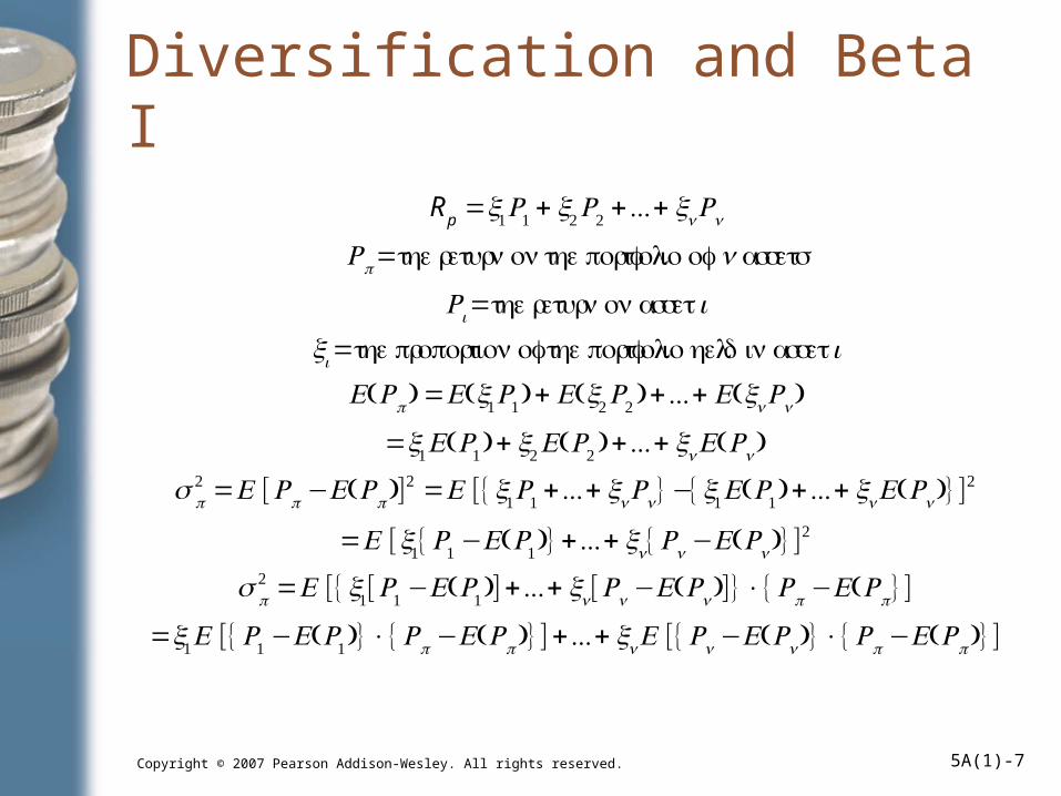
Diversification and Beta I

Rp=x1R1 + x2R2 +...+ xnRn

Rp= the return on the portfolio of n assets

Ri= the return on asset i

xi= the proportion of the portfolio held in asset iE(Rp) =E(x1R1) + E(x2R2 ) +...+ E(xnRn)

=x1E(R1) + x2E(R2 ) +...+ xnE(Rn)

σ p2 =E [Rp−E(Rp)]

2 =E [{x1R1 +...+ xnRn} −{x1E(R1) +...+ xnE(Rn)} ]2

=E [x1{R1 −E(R1)} +...+ xn{Rn−E(Rn)} ]2

σ p2 =E [{x1[R1 −E(R1)] +...+ xn[Rn−E(Rn)]}×{Rp−E(Rp}]

=x1E [{R1 −E(R1)}×{Rp−E(Rp)} ] +...+ xnE [{Rn−E(Rn)}×{Rp−E(Rp)} ]


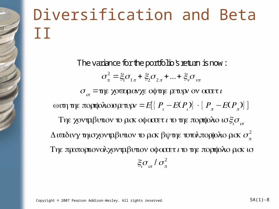
Diversification and Beta II

The variance for the portfolio's return is now:

σ p2 =x1σ1p + x2σ 2 p +...+ xnσ np

σ ip =the covariance of the return on asset i

with the portfolio's return = E[{Ri −E(Ri )}×{Rp−E(Rp)} ]

The contribution to risk of asset i to the portfolio is xiσ ip

Dividing this contribution to risk by the total porfolio risk σ p2

The proportional contribution of asset i to the portfolio risk is xiσ ip / σ p

2


Diversification and Beta II (cont’d)

The higher the ratio, the more the

value of the asset

moves with changes in the value of the porfolio,

and the more asset i contributes to portfolio risk.

The marginal contribution of an asset

to the risk of a portfolio

depends not on the risk of the asset in isolation,

but on the sensitivity of that

asset's return to changes in the value of the portfolio


Diversification and Beta III

im2m

im2m

market portfolio =

is called asset 's beta

Beta is a measure of the asset's marginal contribution to the

risk of the market portfolio

A higher beta means that an asset's return is m

i

p m

iσσ

σβ σ

=

=

ore sensitiveto change in the value of the market portfolio and that the

asset contributes more to the risk of the portfolio


Diversification and Beta IV

The return on asset i can be considered as made up of two components

One that moves with the market's return (Rm

)

And a random factor with expected value of zero that is unique to

the asset (ε i ) and is uncorrelated with the market returnRi =αi +βiRm+ε i ⇒ E(Ri ) =αi +βiE(Rm)Calculating the covariance of asset i's return

σ im=E[{Ri −E(Ri )}×{Rm−E(Rm)} ]

=E [{βi[Rm−E(Rm)] +ε i}×{Rm−E(Rm)} ]Since ε i is uncorrelated with Rm,E [{ε i}×{Rm−E(Rm)} ] =0

σ im=βiσm2

Dividing both sides by σm2 ⇒ βi =

σ im

σm2

Which is the same as the algebraic derivation


Systematic and Nonsystematic Risk I

The variance of asset i's return is calculated as:

σ i2 =E [Ri −E(Ri )]

2 =E [βi{Rm−E(Rm)} +ε i ]2

Since ε i is uncorrelated with the market return:

σ i2 =βi

2σm2 +σ ε

2

βi2σm

2 is related to market risk and called systematic risk

σ ε2 is unique to the asset and called nonsystematic risk

Systematic risk cannot be diversified awayNonsystematic is the risk that is eliminated by diversification


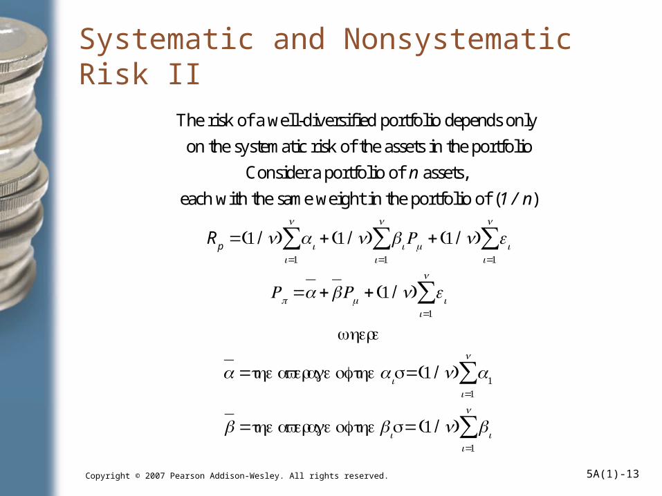
Systematic and Nonsystematic Risk II

The risk of a well-diversified portfolio depends only

on the systematic risk of the assets in the portfolio

Consider a portfolio of n assets,

each with the same weight in the portfolio of (1 / n)

Rp=(1 / n) αi +(1 / n) βiRm+(1 / n) ε i

i=1

n

∑i=1

n

∑i=1

n

∑

Rp =α +βRm+(1 / n) ε ii=1

n

∑where

α =the average of the αis=(1 / n) α1i=1

n

∑

β =the average of the βis = (1 / n) βii=1

n

∑


Systematic and Nonsystematic Risk II (cont’d)

If the portfolio is well diversifed so that the ε is are uncorrelated with each other and with the market return

σ p2 =β2σm

2 +(1 / n)(average variance of ε i )

As n gets large, (1 / n)(average variance of ε i ) gets very small

A well-diversifed portfolio has a risk of β2σm2 ,

which is only related to systematic risk


Capital Asset Pricing Model (CAPM)

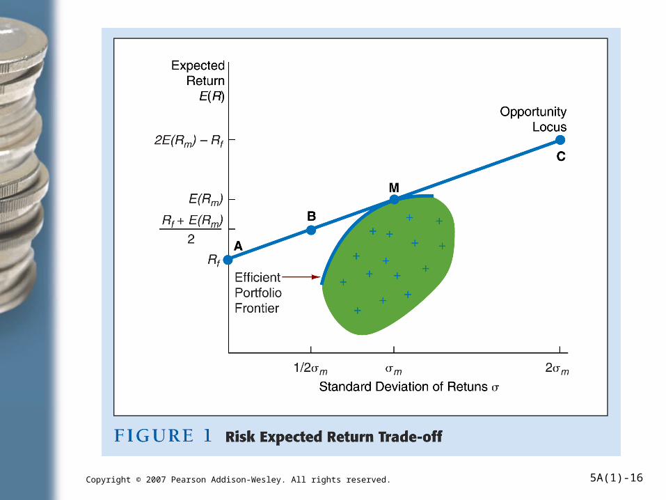
• Shaded area shows combinations of standard deviation and expected return for various portfolios with differing levels of risk

• The most attractive combinations for the risk-averse investor are on the heavy line, the efficient portfolio frontier

• Choosing different combinations an investor can form a portfolio that lies anywhere on the line A-C


Capital Asset Pricing Model (CAPM) (cont’d)

• M is chosen so that it is tangent to the efficient portfolio frontier

• The line is the opportunity locus, the best combination of standard deviations and expected returns available to the investor

• Assumes that all investors have the same assessment of the expected returns and standard deviations of all assets

• Therefore portfolio M and the market portfolio are the same


CAPM Equation

The trade-off between expected returns and increased risk is given by

the slope of the opportunity locus E(Rm

)−RfWhen an investor is willing to increase the risk of the portfolio by σm,

then an additional expected return of E(Rm)−Rf is gained

The market price of a unit of market risk σm

is E(Rm)−Rf → The Market Price of Risk

βi is the marginal contribution of asset i to a portfolio's riskThe amount an asset's expected return exceeds the risk-free rate

should equal the market price of the risk times the marginal contribution of that asset to portfolio risk

The CAPM asset pricing relationship is:E(Ri ) =Rf +βi[E(Rm)−Rf ]


Security Market Line

• The expected return that the market sets for a security given its beta

• Beta of 1.0 marginal contribution to a portfolio’s risk is the same as the market so it should be priced to have the same expected return as the market portfolio

• An asset should be priced so that it has a higher expected return not when it has a greater risk in isolation, but rather when its systematic risk is greater


Arbitrage Pricing Theory

• There can be several sources of systematic risk that cannot be eliminated through diversification

• Factors related to inflation, aggregate output, default risk premiums and/or the term structure of interest rates

• Same basic conclusion as CAPM—an asset should be priced so that it has a higher expected return when its systematic risk is greater

Ri=βi

1(factor 1)+βi2(factor 2)+...+ βi

k(factor k) +ε iSometimes called the k-factor model, the βis are the sensitivity of asset i's return to each of these factorsThe market price for each factor j is E(Rfactorj )−Rf

The expected return on a security is

E(Ri ) =Rf +βi1[E(Rfactor 1)−Rf ] + ...+ βi

k[E(Rfactor k)−Rf ]

Appendix 1 to Chapter 5 Models of Asset Pricing. Copyright © 2007 Pearson Addison-Wesley. All...

Documents

Transcript of Appendix 1 to Chapter 5 Models of Asset Pricing. Copyright © 2007 Pearson Addison-Wesley. All...