2012 South Florida Environmental Report Appendix 1-6

App.1-6-1

Appendix 1-6: South Florida Water Depth

Assessment Tool Jason Godin

INTRODUCTION

Persistent drought conditions over the past few years have made it critical for resource management and water supply purposes to understand present (real-time) and historical hydrologic conditions in the South Florida environment from a regional spatial perspective. Additionally, there is an ongoing need for this type of information on a year-round basis for operational decision support during flood events as well as normal conditions to improve the routing of water for water supply needs and environmental benefits. The South Florida Water Depth Assessment Tool (SFWDAT) was developed by the South Florida Water Management District (SFWMD or District) as a resource management tool to illustrate the present “state of the system.” The two primary purposes of the SFWDAT are to (1) provide a greater understanding of the spatial and temporal dynamics of water depths across entire ecosystems [e.g., wetlands, lakes, aquifers (groundwater)], and (2) provide access readily to real-time water depth data and water depth-based indices for use by agency staff and various stakeholders.

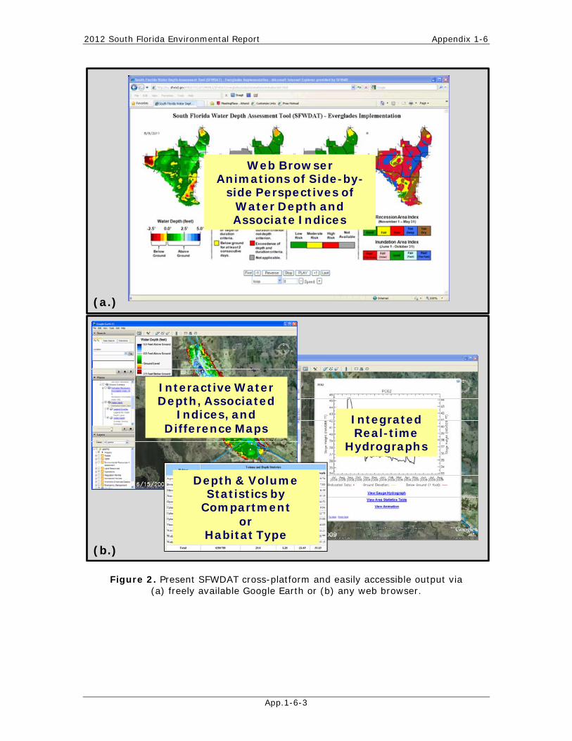
In partnership with the SFWMD, hundreds of real-time water level gauges throughout the District’s boundaries are managed by several government agencies including the Everglades National Park (ENP or Park), U.S. Geological Survey (USGS), and the U.S. Army Corps of Engineers (USACE). The SFWDAT couples these water level gauges to produce spatially continuous estimates of mean daily surface water elevations for nine hydrologically distinct basins of the Everglades Protection Area (EPA), Lake Okeechobee, and a partially restored portion of the Kissimmee River floodplain known as Pool C (Figure 1). Water depth surfaces are calculated by subtracting known ground elevations (or gridded elevation models) from these water elevation surfaces. The primary near real-time based outputs of the SFWDAT include:

• Animated side-by-side: Internet browser-based one-year retrospective (Figure 2, Panel a), and

• Static interactive, through Google Earth, spatial perspectives of water depth and depth-related indices over each of the three present implementation regions (Figure 2, Panel b).

Appendix 1-6 Volume I: The South Florida Environment

App. 1-6-2

Figure 1. Current South Florida Water Depth Assessment Tool (SFWDAT) implementations for (a) Pool C of the Kissimmee floodplain, (b) Lake Okeechobee, and (c) the Everglades Protection Area (EPA) relative to the South Florida Water Management District boundaries and overlaid with stage monitoring locations.

(Also, see Figure 1-1 of this volume for general District boundary map.)

WCA -1

WCA-3A

WCA-2B

WCA -2A

WCA-3B

ENP

BCNP / Pi cayune

Rotenberger WMA

Holey Land WMA

(b)

(a)

(c)

2012 South Florida Environmental Report Appendix 1-6

App.1-6-3

Figure 2. Present SFWDAT cross-platform and easily accessible output via (a) freely available Google Earth or (b) any web browser.

Web Browser Animations of Side-by-

side Perspectives of Water Depth and Associate Indices

(a.)

Integrated Real-time

Hydrographs

Interactive Water Depth, Associated

Indices, and Difference Maps

Depth & VolumeStatistics by

Compartment or

Habitat Type(b.)

Appendix 1-6 Volume I: The South Florida Environment

App. 1-6-4

THEORY AND METHODS

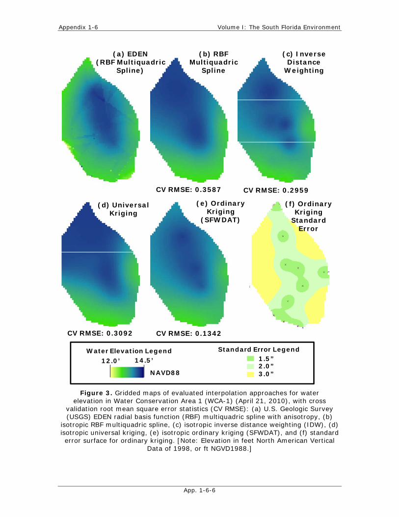
Many of the works of the South Florida Water Management District revolve around the management and operations of water resources for water supply and flood control purposes. The Central and South Florida regional flood control system (C&SF System) connects and regulates a series of lakes, rivers and wetland systems through a network of canals and water control structures (see Chapter 2 of this volume). Integrated within the C&SF System are various large-scale ecosystem restoration initiatives and projects, such as the Comprehensive Everglades Restoration Plan (CERP) and Kissimmee River Restoration Project. The management of water for these projects, as well as key bodies of water, such as Lake Okeechobee, benefit from the availability of real-time and historical water depth information produced by the SFWDAT. In addition to supporting the real-time management of the C&SF System, the SFWDAT provides technical support to other District activities such as planning and evaluation, operational decision making, permit-related support, emergency management, and communications/outreach.

The original vision behind the agency’s development of the SFWDAT was to provide a spatiotemporal-based, near real-time, decision support system comprised of water depth and a few key performance indicators for the nine wetland basins that make up the more than 2.3 million acres of the Everglades Protection Area (EPA), which includes Water Conservation Areas (WCAs) 1, 2A, 2B, 3A, and 3B, and Everglades National Park (ENP or Park); Big Cypress National Preserve (BCNP) / Picayune Strand Complex; and the Holey Land and Rotenberger Wildlife Management Areas (WMA) (Figure 1, Panel c). The basis of this application was to interconnect the telemetry network of hundreds of surface water and groundwater level gauges existing throughout the system. The principal objective was to develop a relatively simple application framework and methodology that could be automated daily to support adaptive management and associated operational decision support. The SFWDAT application was developed to support these objectives using the Interactive Data Language™ of ITT Visual Information Solutions, which is a rapid development environment that includes a comprehensive library of graphical routines. The primary functions and order of operations of this automated application tool include the following:

1. Acquire data of breakpoint (irregular sampling intervals based on change detection) and daily average water levels from SFWMD and USGS (National Water Inventory System, or NWIS) time series-based database systems of hydrologic monitoring information;

2. Integrate breakpoint data into daily mean water levels and data quality assessment; 3. Fill temporal gaps based on point-to-point regressions for short-term gaps and a

correlation approach based on adjacent gauges for longer-term gaps (performance ranked correlation matrix),

4. Interpolate surfaces of mean daily water elevations for the previous year for each basin independently;

5. Calculate mean daily water depth surfaces by displacing ground elevation from the water elevation surfaces and calculate depth and duration related performance metrics; and

6. Produce spatiotemporal graphical, statistical tables and code-based output for Google Earth and web browser-accessible animations.

The interpolation of water elevation surfaces from water level gauges is the key process that allows the SFWDAT to paint a spatial perspective of regional water elevations in relation to land surface (water depth). Likewise, the diverse series of pathways available under the multifaceted field of geostatistical analysis offers a range of approaches to producing conceptually the same gridded water elevation surface product. Initially, the SFWMD considered several different interpolation approaches, but eventually focused attention on the kriging suite of interpolators.

2012 South Florida Environmental Report Appendix 1-6

App.1-6-5

While there were several factors involved with selecting a consistent and simplistic approach to automating a geostatistical methodology, there was also an ongoing effort by the USGS to develop a similar type of product to support research activities of CERP. This effort, known as the Everglades Depth Estimation Network (EDEN; Palaseanu and Pearlstine 2008), also shares the goal of providing surfaces of water elevation and depths for a subset of the EPA. The EDEN products are based on a global, meaning across basins with boundary conditions, radial basis function (RBF), multiquadric spline interpolation methodology with customized boundary conditions.

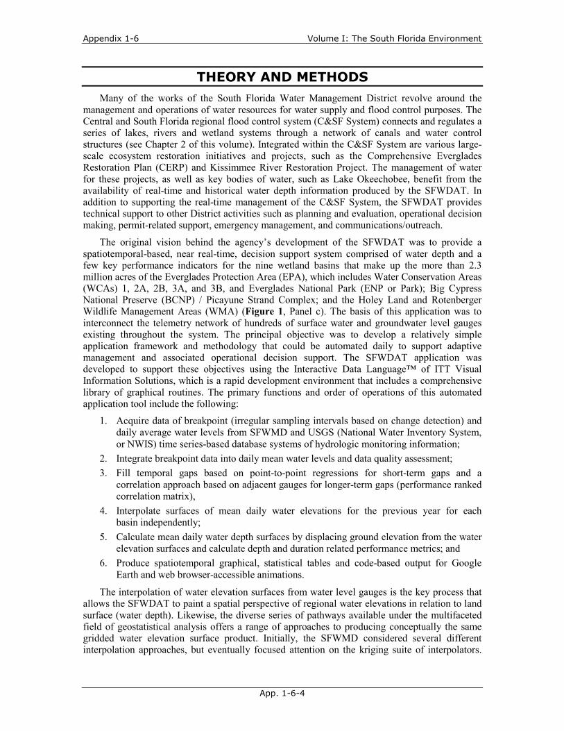
The SFWDAT effort evaluated several common interpolation approaches such as inverse distance weighting (IDW), the RBF multiquadric spline, universal kriging (also known as kriging with an external drift) and ordinary kriging to identify a geostatistical methodology that could be implemented in a consistent manner across each of the hydrologically distinct basins of the EPA; as an example, see the side-by-side comparison of these approaches to WCA-1 in Figure 3 with associated cross validation Root Mean Square Error (RMSE) statistics. The direct output surfaces from the USGS EDEN program, available on the USGS website at http://sofia.usgs.gov/eden/models/watersurfacemod.php, was also evaluated as a candidate product for implementation into the SFWDAT (Figure 3, Panel a).

The selection of a geostatistical interpolation approach was narrowed down using three key principal criteria: (1) qualitative functional alignment, such as matching observed hydropatterns and adequately capturing the naturally smooth gradients of water surfaces in these basins, (2) minimal surface uncertainty (cross validation) and the ability to quantify interpolation uncertainty and (3) validation performance. The evaluation focused on the isotropic (omni-directional), basin-specific (independent interpolations for each basin), kriging approaches with no nugget value, (i.e., no forced sampling error) principally due to misrepresentations by the other interpolation approaches to capture the relatively homogenous or flat water elevations in impounded areas such as WCA-1. These surface anomalies were clearly present in each of the other interpolation approaches, such as edge undulations exhibited in the water elevation cross sectional perspectives presented in Figure 4. In this example, the universal kriging approach most appropriately captured the flat-pool like surface of this basin, but exhibited higher cross validation RMSE than the ordinary kriging. Also, the universal kriging method was significantly more complex to implement as an automated and uniform approach due to the process of fitting an additional number of parameters, which is the basis of removing polynomial (e.g., quadratic) trend surfaces prior to the kriging process. As such, the selection of the ordinary kriging methodology as the principal interpolation approach for SFWDAT follows the logic of keeping the methodology as simple as possible, while still producing an acceptable quality of results. This is especially true when the simpler process produces the same or better results (lower RMSE) than the more complex universal kriging approach. The lower cross validation RMSE of the ordinary kriging approach in this case is in part due to the relatively high density of water level monitoring gauges available to the SFWDAT in these areas. A case could be made for universal kriging in areas where less densely populated gauge networks are unable to capture the “neighborhood” autocorrelation patterns intrinsic to each basin. Some areas of the ENP and BCNP may be good candidates for this more complex approach or if monitoring networks are reduced under future circumstances.

Appendix 1-6 Volume I: The South Florida Environment

App. 1-6-6

Figure 3. Gridded maps of evaluated interpolation approaches for water elevation in Water Conservation Area 1 (WCA-1) (April 21, 2010), with cross

validation root mean square error statistics (CV RMSE): (a) U.S. Geologic Survey (USGS) EDEN radial basis function (RBF) multiquadric spline with anisotropy, (b)

isotropic RBF multiquadric spline, (c) isotropic inverse distance weighting (IDW), (d) isotropic universal kriging, (e) isotropic ordinary kriging (SFWDAT), and (f) standard error surface for ordinary kriging. [Note: Elevation in feet North American Vertical

Data of 1998, or ft NGVD1988.]

(a) EDEN(RBF Multiquadric

Spline)

(b) RBF Multiquadric

Spline

(c) InverseDistance

Weighting

(e) OrdinaryKriging

(SFWDAT)

NAVD88

1.5”2.0”3.0”

(d) Universal Kriging

(f) OrdinaryKriging

Standard Error

12.0’ 14.5’Water Elevation Legend Standard Error Legend

CV RMSE: 0.3587 CV RMSE: 0.2959

CV RMSE: 0.3092 CV RMSE: 0.1342

2012 South Florida Environmental Report Appendix 1-6

App.1-6-7

Figure 4. Cross-sectional water elevation profiles of evaluated interpolation methodologies for WCA-1: (a) USGS EDEN RBF multiquadric dpline with anisotropy, (b) isotropic RBF multiquadric spline, (c) isotropic IDW, (d) isotropic universal kriging, and (e) isotropic ordinary kriging (SFWDAT).

a.

b.

c .

d.

a. b. c . e.d.

e.

Appendix 1-6 Volume I: The South Florida Environment

App. 1-6-8

With varying ranges of water elevation levels across each basin of the EPA, the results of the ordinary kriging interpolation methodology are specifically linked to a best-fit model of spatial dependency or, in this case, the semivariance for each set of data values within a basin. A semivariance model is simply a regression model of all combinations of observed water elevation differences plotted by their spatial distance. The model of these plots, or variogram, is the basis of how the kriging algorithm uses the observed water elevations to predict unknown water elevations at locations throughout a corresponding area, e.g., a basin.

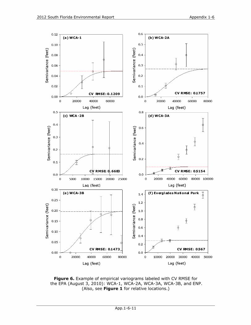
In the development of the SFWDAT, several different variogram models were evaluated to be utilized as a consistent approach to modeling the basin specific spatial dependency. This included the evaluation of spherical, exponential, and Gaussian-based regression models of the empirically based water level semivariance data. The Gaussian model consistently provided the best fit and also aligned with findings by Kumar and Remadev (2006) on the use of Gaussian-based kriging for the interpolation of ground water levels. As such, the Gaussian model was selected as the standard variogram model to be utilized by the SFWDAT. The Gaussian variogram models were also truncated to focus on the mean variability of the local neighboring gauges/variance range instead of the longer range global gradients that were exhibited by the larger basins such as WCA-3A (Figure 5). Variogram model fits of longer range gradients tend to misrepresent the shorter lag variances or more specifically the distance lags that are most common to interpolations of water elevations in these basins due to their relatively high density of monitoring locations. Consequently, the variogram range for each basin was fit to the mean local variance (typically a neighborhood of 8-12 gauges) instead of the range for the overall variance of the water elevations for the whole basin, which often exhibited a range of different scales. Example empirical semivariance and associated Gaussian model regressions are plotted in the variograms for each of the basins of the EPA in Figures 6 and 7 for a single day.

The process of modeling the semivariance (variogram) for each basin, also allows for the ability to utilize these models to spatially characterize the uncertainty or standard error associated with the use of these models as a function of the distance from an observed monitoring location. As such the greater the distance from a monitoring location, the greater the amount of error one could expect from the interpolation. With respect to our earlier example of interpolation methodologies the associated ordinary kriging standard error map for WCA-1 is exhibited in Figure 3, Panel f. While a composite perspective of the interpolated water elevation and variogram (Figures 6 and 7) based standard error maps for the EPA for a single day (August 11, 2010) are presented in Figure 8, Panels a and b.

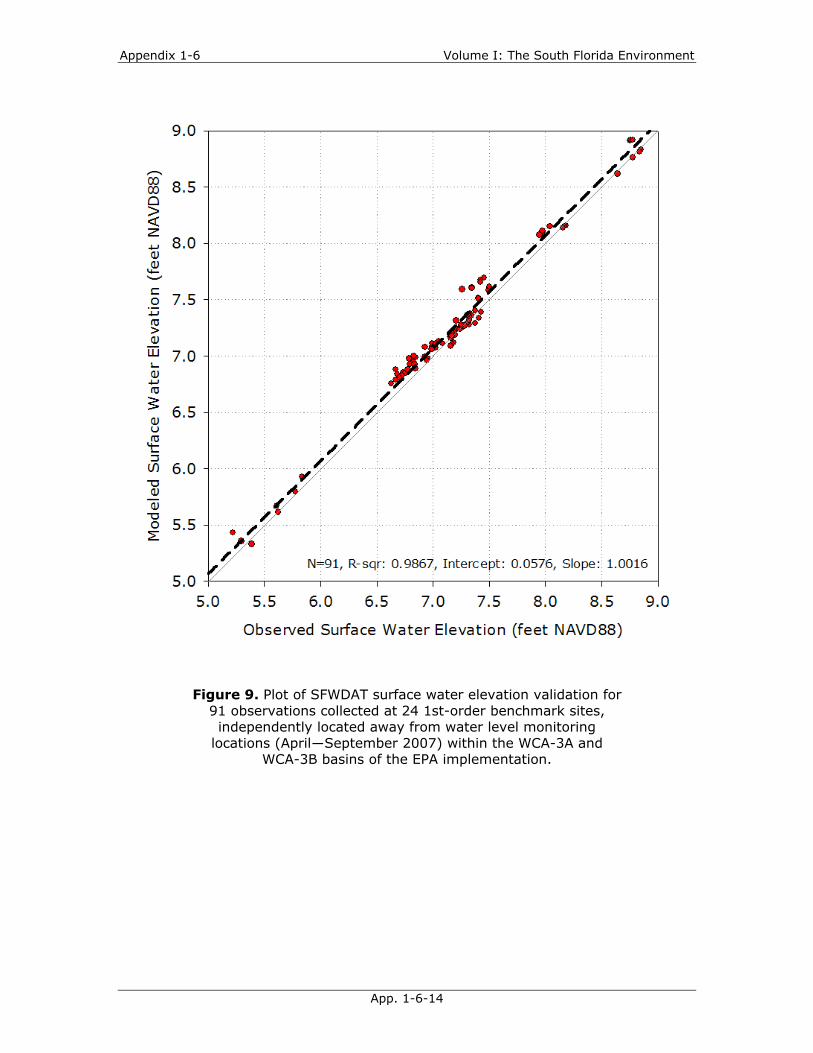
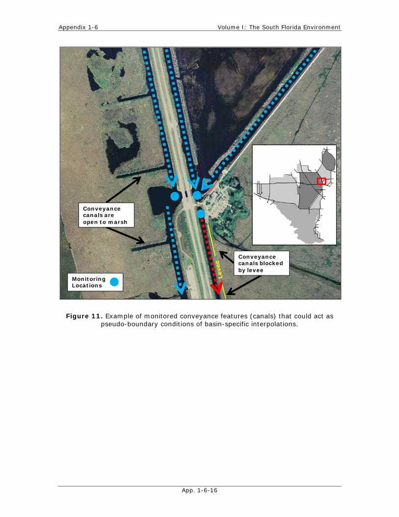
Fortunately, the District also had access to a water elevation validation dataset sponsored by the USGS EDEN program. In this case, researchers at the University of Connecticut collected precise water elevation measurements at 24 first-order benchmark sites independently located away from water level monitoring locations (April–September 2007) within the WCA-3A and WCA-3B basins of the EPA (Volin et al., 2008) for comparison with gridded water elevation surfaces produced by the EDEN program (EDEN validation document available at http://digitalcommons.uconn.edu/cgi/viewcontent.cgi?article=1007&context=nrme_articles). These measurements also provided valuable insights into the performance of the SFWDAT ordinary kriging approach in these basins. As shown in Figure 9, there was a very strong correlation between the observed and modeled water elevations with very little bias (R2: 0.9867, intercept: 0.0576”, and slope of 1.0016). Likewise, the spatial distribution of errors or the mean absolute deviation was fairly consistent at the interior benchmarks and higher along the basin edges as expected (Figure 10). The fact that the higher errors were along the basin boundaries warrants future investigation into the use of imposing boundary conditions where unconstrained (open to surrounding marsh) conveyance features, such as monitored canals, could provide additional interpolation network support (see Figure 11). Overall, the observed 95 percent

2012 South Florida Environmental Report Appendix 1-6

App.1-6-9

confidence range in these two basins was better than 2 in or 0.17 ft. This level of precision was consistent with the typical standard error maps for these basins, as shown in Figure 9, Panel b.

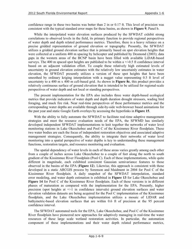
While the interpolated water elevation surfaces produced by the SFWDAT exhibit strong correlations to observed levels in the field, its primary function to provide regional perspectives of water depth and depth related performance metrics. Therefore, there is a heavy reliance on a precise gridded representation of ground elevation or topography. Presently, the SFWDAT utilizes a gridded ground elevation surface that is primarily based on spot elevation heights that were collected at a uniform 400 m spacing by helicopter and published by Desmond (2003); data gaps in the western areas of the BCNP basin have been filled with available LiDAR-based surveys. The 400 m spaced spot heights are published to be within a +/-0.5 ft confidence interval based on an adjacent validation effort. To couple these relatively high estimated levels of uncertainty in ground elevation estimates with the relatively low uncertainly estimates in water elevation, the SFWDAT presently utilizes a version of these spot heights that have been smoothed by ordinary kriging interpolation with a nugget value representing 0.5 ft level of uncertainty to a 400 m x 400 m cell-based grid. As shown in Figure 8c, this product provides a relatively continuous surface of ground elevation that is intended to be utilized for regional-scale perspectives of water depth and not local or standing perspectives.

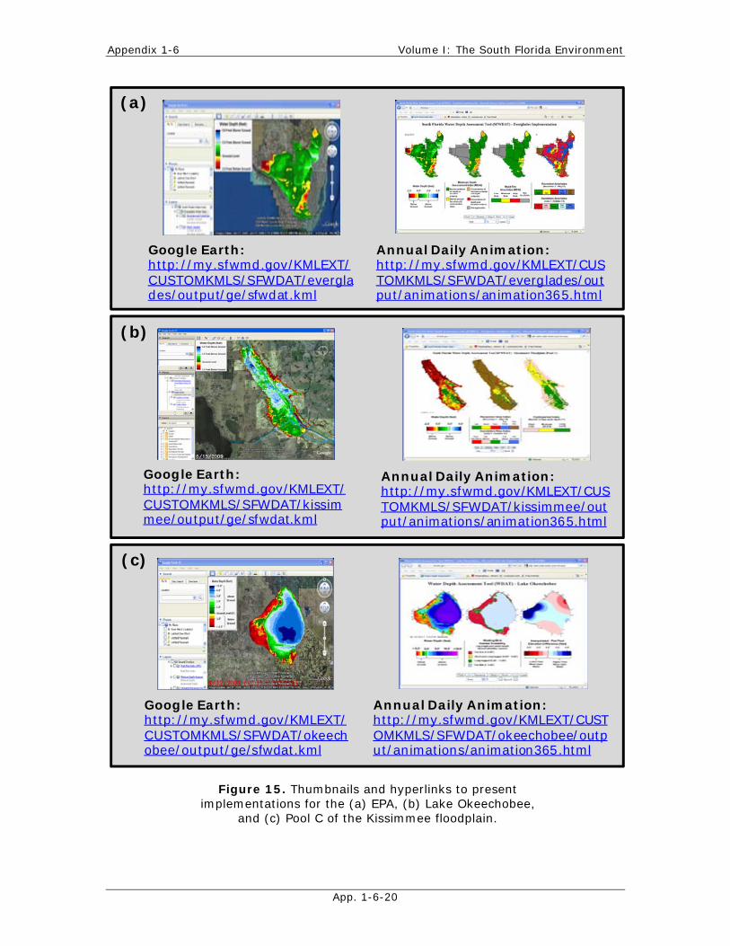
The present implementation for the EPA also includes three water depth-based ecological metrics that provide indicators of water depth and depth duration drought stressors, wading bird foraging, and muck fire risk. Near real-time perspectives of these performance metrics and the corresponding water depths are available through side-by-side web-browser based animations for the past year and static Google Earth overlays by accessing the hyperlinks in Figure 15.

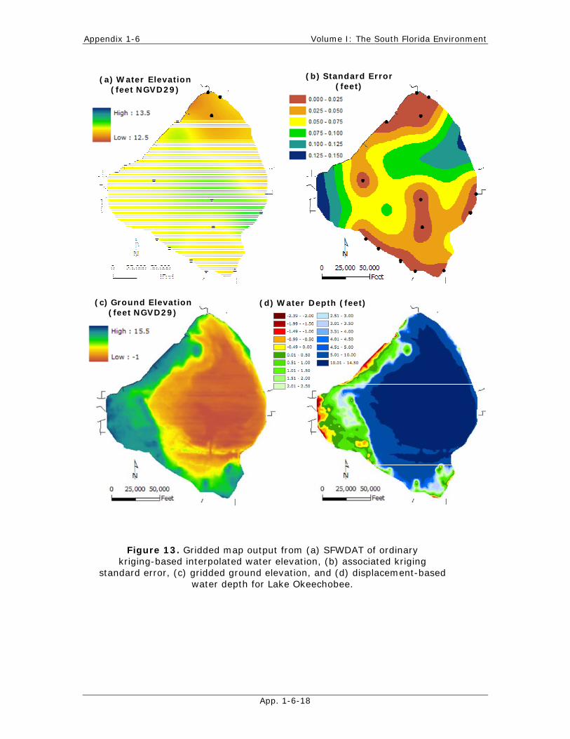
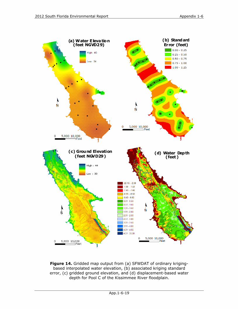
With the ability to fully automate the SFWDAT to facilitate real-time adaptive management strategies and meet the resource evaluation needs of the EPA, the SFWMD has similarly developed independent SFWDAT implementations to knit together the networks of water level monitoring stations in Lake Okeechobee and Pool C of the Kissimmee River floodplain. These two water bodies are each the focus of independent restoration objectives and associated adaptive management strategies. Consequently, the ability to integrate their networks of water level monitoring into a spatial perspective of water depths is key to understanding these management functions, restoration targets, and resource monitoring and evaluation.

The spatial dependency of water levels in each of these areas varies greatly among each other from a couple of inches across Lake Okeechobee to a couple of feet along the north to south gradient of the Kissimmee River Floodplain (Pool C). Each of these implementations, while quite different in magnitude, each exhibited consistent Gaussian semivariance features to those observed in the basins of the EPA (Figure 12). Likewise, this approach is consistent with those developed in a static ARCGIS process by Sorenson and Maidment in 2004 for Pool C of the Kissimmee River floodplain. A daily snapshot of the SFWDAT interpolation, standard error modeling, and water depth estimation is exhibited in Figure 13 for Lake Okeechobee and Figure 14 for Pool C of the Kissimmee River floodplain. Each of these versions is in different phases of maturation as compared with the implementation for the EPA. Presently, higher precision (spot heights at +/-1 in confidence intervals) ground elevation surfaces and water elevation validation datasets are being acquired for the Pool C implementation of the Kissimmee floodplain, and the Lake Okeechobee implementation utilizes a mosaic of LIDAR and bathymetric-based elevation surfaces that are within 0.6 ft of precision at the 95 percent confidence interval.

The SFWDAT automated tools for the EPA, Lake Okeechobee, and Pool C of the Kissimmee River floodplain have pioneered new approaches for adaptively managing in real-time the water resources of these large scale wetland restoration activities. In particular, the automation component of these implementations and their water depth related performance metrics,

Appendix 1-6 Volume I: The South Florida Environment

App. 1-6-10

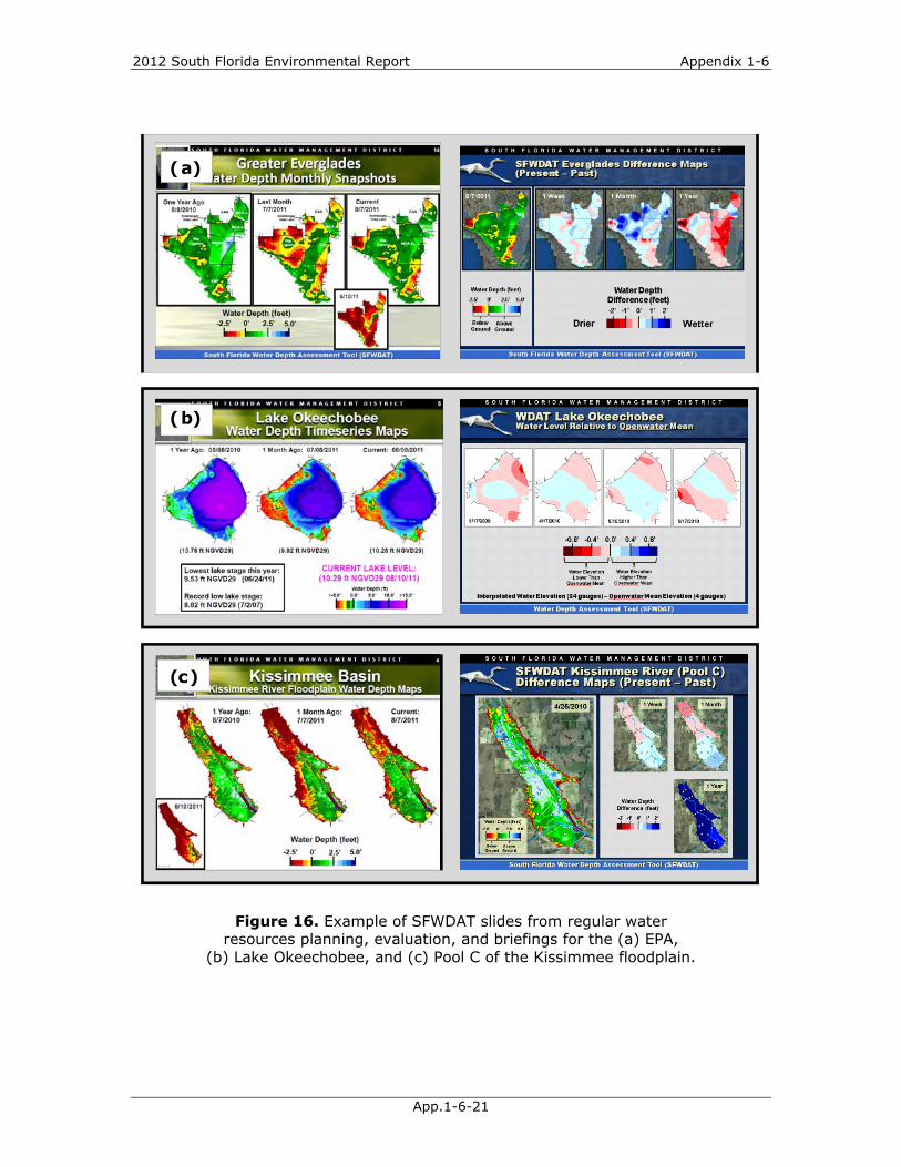
combined with the ease of accessibility to interact with the SFWDAT output through web-browser based animations and the Google Earth environment (see thumbnails with hyperlinks in Figure 15 that provides daily updated static and animated products) have provided significant cost savings for data processing and assimilation efforts associated with regular resource evaluation meetings and reporting (example reporting products in Figure 16), and communication with both internal and external stakeholders.

Figure 5. Example of local and global Gaussian variogram model fits for Everglades National Park (ENP or Park); global models

misrepresent local variance ranges.

Global Fit

L ocal Fit

Global Fit

Local F it

2012 South Florida Environmental Report Appendix 1-6

App.1-6-11

Figure 6. Example of empirical variograms labeled with CV RMSE for the EPA (August 3, 2010): WCA-1, WCA-2A, WCA-3A, WCA-3B, and ENP.

(Also, see Figure 1 for relative locations.)

(a) WCA-1 (b) WCA-2A

(c) WCA -2B (d) WCA-3A

(f) Everglades National Park(e) WCA-3B

CV RMSE: 0.1209

CV RMSE: 0.5154

CV RMSE: 0.1473

CV RMSE: 0.6683

CV RMSE: 0.1757

CV RMSE: 0.567

Appendix 1-6 Volume I: The South Florida Environment

App. 1-6-12

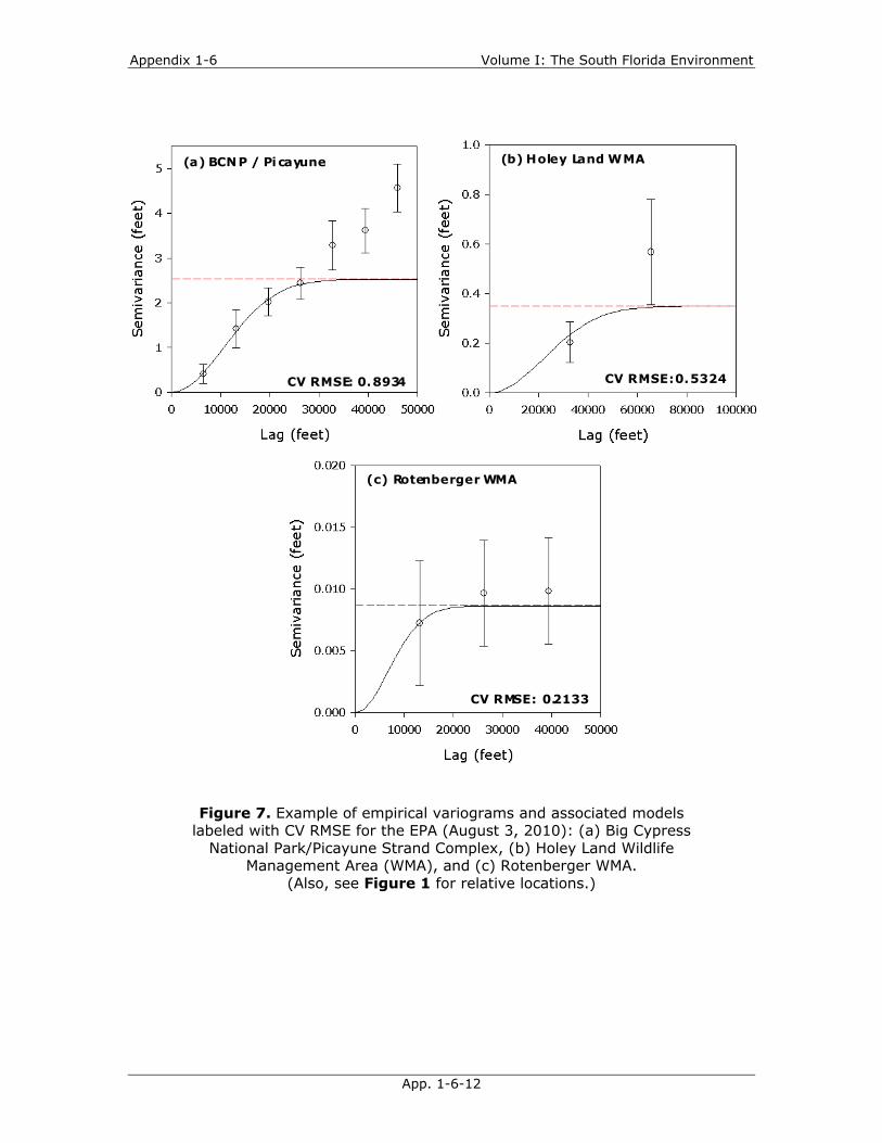
Figure 7. Example of empirical variograms and associated models labeled with CV RMSE for the EPA (August 3, 2010): (a) Big Cypress

National Park/Picayune Strand Complex, (b) Holey Land Wildlife Management Area (WMA), and (c) Rotenberger WMA.

(Also, see Figure 1 for relative locations.)

(a) BCNP / Pi cayune

(c) Rotenberger WMA

(b) Holey Land WMA

CV RMSE: 0.5324CV RMSE: 0.8934

CV RMSE: 0.2133

2012 South Florida Environmental Report Appendix 1-6

App.1-6-13

Figure 8. Gridded map output from the SFWDAT (August 3, 2010): (a) ordinary kriging-based interpolated water elevation, (b) associated kriging

standard error, (c) gridded ground elevation, and (d) displacement-based water depth for the nine independent basins of the EPA.

(a) Water Elevation (feet NAVD88)

(b) Standard Error(feet)

(c) Ground Elevation (feet NAVD88) (d) Water Depth (feet)

Appendix 1-6 Volume I: The South Florida Environment

App. 1-6-14

Figure 9. Plot of SFWDAT surface water elevation validation for 91 observations collected at 24 1st-order benchmark sites, independently located away from water level monitoring

locations (April―September 2007) within the WCA-3A and WCA-3B basins of the EPA implementation.

2012 South Florida Environmental Report Appendix 1-6

App.1-6-15

Figure 10. Map of the mean absolute deviation of SFWDAT surface water elevation from 91 observations collected at 24 1st-order

benchmark sites (April―September 2007) relative to water level monitoring locations (denoted with an “X”) within the WCA-3A and

WCA-3B basins of the EPA implementation.

Appendix 1-6 Volume I: The South Florida Environment

App. 1-6-16

Figure 11. Example of monitored conveyance features (canals) that could act as

pseudo-boundary conditions of basin-specific interpolations.

Monitoring Locations

Conveyance canals blocked by levee

Conveyance canals are open to marsh

2012 South Florida Environmental Report Appendix 1-6

App.1-6-17

Figure 12. Example empirical variograms and associated models labeled with CV RMSE for (a) Lake Okeechobee and (b) Pool C of the

Kissimmee floodplain. (Also, see Figure 1 for relative locations.)

(a) Lake Okeechobee

(b) Pool C KissimmeeRiver Floodplain

CV RMSE: 1.162

CV RMSE: 0.1603

Appendix 1-6 Volume I: The South Florida Environment

App. 1-6-18

(b) Standard Error(feet)

(a) Water Elevation (feet NGVD29)

(d) Water Depth (feet)(c) Ground Elevation (feet NGVD29)

Figure 13. Gridded map output from (a) SFWDAT of ordinary kriging-based interpolated water elevation, (b) associated kriging

standard error, (c) gridded ground elevation, and (d) displacement-based water depth for Lake Okeechobee.

2012 South Florida Environmental Report Appendix 1-6

App.1-6-19

Figure 14. Gridded map output from (a) SFWDAT of ordinary kriging-based interpolated water elevation, (b) associated kriging standard

error, (c) gridded ground elevation, and (d) displacement-based water depth for Pool C of the Kissimmee River floodplain.

(b) Standard Error (feet)

(a) Water Elevation (feet NGVD29)

(d) Water Depth (feet)

(c) Ground Elevation(feet NGVD29)

Appendix 1-6 Volume I: The South Florida Environment

App. 1-6-20

Google Earth: http://my.sfwmd.gov/KMLEXT/CUSTOMKMLS/SFWDAT/everglades/output/ge/sfwdat.kml

Google Earth: http://my.sfwmd.gov/KMLEXT/CUSTOMKMLS/SFWDAT/okeechobee/output/ge/sfwdat.kml

Annual Daily Animation: http://my.sfwmd.gov/KMLEXT/CUSTOMKMLS/SFWDAT/kissimmee/output/animations/animation365.html

Google Earth: http://my.sfwmd.gov/KMLEXT/CUSTOMKMLS/SFWDAT/kissimmee/output/ge/sfwdat.kml

Annual Daily Animation: http://my.sfwmd.gov/KMLEXT/CUSTOMKMLS/SFWDAT/okeechobee/output/animations/animation365.html

Annual Daily Animation: http://my.sfwmd.gov/KMLEXT/CUSTOMKMLS/SFWDAT/everglades/output/animations/animation365.html

(a)

(b)

(c)

Figure 15. Thumbnails and hyperlinks to present implementations for the (a) EPA, (b) Lake Okeechobee,

and (c) Pool C of the Kissimmee floodplain.

2012 South Florida Environmental Report Appendix 1-6

App.1-6-21

Figure 16. Example of SFWDAT slides from regular water resources planning, evaluation, and briefings for the (a) EPA,

(b) Lake Okeechobee, and (c) Pool C of the Kissimmee floodplain.

(a)

(b)

(c)

Appendix 1-6 Volume I: The South Florida Environment

App. 1-6-22

LITERATURE CITED

Cressie, N. 1993. Statistics for Spatial Data. John Wiley & Sons, Inc., New York, NY.

Desmond, G.D. 2003. Measuring and Mapping the Topography of the Florida Everglades for Ecosystem Restoration. U.S. Geological Survey Fact Sheet 021-03.

Kumar, V. and Remadevi. 2006. Kriging of Groundwater Levels – A Case Study. Journal of Spatial Hydrology, Vol. 6, No. 1, Spring 2006.

Palaseanu, M. and L. Pearlstine. 2008. Estimation of Water Surface Elevations for the Everglades, Florida. Computers and Geosciences, 34(7): 815-826.

Sorenson, J.K. and D. R. Maidment. 2004. Temporal Geoprocessing for Hydroperiod Analysis of the Kissimmee River, CRWR Online Report 04-5, Center for Research in Water Resources, University of Texas at Austin, TX.

Volin, J., Z. Liu, A. Higer, F. Mazzotti, D. Owen, J. Allen and L. Pearlstine. 2008, Validation of a Spatially Continuous EDEN Water-Surface Model for the Everglades, Florida. Department of Natural Resources Management and Engineering, University of Connecticut, CT.