APPARATUS DETAILS FOR TRIAXIAL TESTING - …jrlai/CE7334/Unit5.pdf · Department of Construction...
43
Department of Construction Engineering Advanced Geotechnical Laboratory Chaoyang University of Technology -- Triaxial Apparatus -- 1 APPARATUS DETAILS FOR TRIAXIAL TESTING Prepared by Dr. Roy E. Olson on Fall 1989 Modified by Jiunnren Lai on Spring 2004 ______ INTRODUCTION Full consideration of all relevant aspects of triaxial testing involves so much material, of such diversified types, that it was not convenient to include the material at the same time that general triaxial testing techniques were covered (Chapter 19). Some of the details are included in this chapter. DEVICES FOR APPLICATION OF LOAD OR DEFORMATION Triaxial tests are usually performed by loading the end of the specimens at a constant rate of deformation but constant load procedures may be used as well. Dead Weight Systems The least expensive loading system involves application of constant loads. In its least expensive form (Fig. 20.1), the device consists of a hanger system made of components available in any hardware store, with dead loads applied using weights. The weights become a problem for capacities much in excess of a few hundred pounds (the loads required for most tests with samples of 1.5-inch diameter). For heavier loads it is typical to construct lever arm systems with mechanical advantages of the order of 10:1. Fig. 20.1 Simple Dead-Weight Loading System
Transcript of APPARATUS DETAILS FOR TRIAXIAL TESTING - …jrlai/CE7334/Unit5.pdf · Department of Construction...
Department of Construction Engineering Advanced Geotechnical Laboratory Chaoyang University of Technology -- Triaxial Apparatus --
1
APPARATUS DETAILS FOR TRIAXIAL TESTING
Prepared by Dr. Roy E. Olson on Fall 1989
Modified by Jiunnren Lai on Spring 2004
______
INTRODUCTION
Full consideration of all relevant aspects of triaxial testing involves so much material, of such diversified types, that it was not convenient to include the material at the same time that general triaxial testing techniques were covered (Chapter 19). Some of the details are included in this chapter.
DEVICES FOR APPLICATION OF LOAD OR DEFORMATION
Triaxial tests are usually performed by loading the end of the specimens at a constant rate of deformation but constant load procedures may be used as well.
Dead Weight Systems The least expensive loading system involves application of constant loads. In its least expensive form (Fig. 20.1), the device consists of a hanger system made of components available in any hardware store, with dead loads applied using weights. The weights become a problem for capacities much in excess of a few hundred pounds (the loads required for most tests with samples of 1.5-inch diameter). For heavier loads it is typical to construct lever arm systems with mechanical advantages of the order of 10:1.
Fig. 20.1 Simple Dead-Weight Loading System

Department of Construction Engineering Advanced Geotechnical Laboratory Chaoyang University of Technology -- Triaxial Apparatus --
2
Dead weight systems are difficult to use. For normally consolidated soils, the compressive strength under undrained conditions is about half of the compressive strength under drained conditions. If a drained test is planned, and half of the real (fully drained) failure load is applied as the first step, the sample fails immediately under undrained conditions. Experience usually is that sample failure occurs prematurely because the last load placed on the sample was too large. The problem is particularly severe with drained tests on highly overconsolidated clays and dense sands because the strength generally decreases with time and a question arises as to when the next load can be applied. Finally, it is difficult to follow the post-failure stress-strain curve if the strength of the sample decreases after failure.
Mechanical Constant Rate of Deformation Devices The majority of triaxial tests are performed using a gear-driven loading press (Fig. 20.2). Presses with capacities up to about 2 tons can be driven with relatively inexpensive variable-speed transmissions and small electric motors. Such presses are readily available and reasonably priced.
Fig. 20.2 Mechanical Constant Rate of Deformation Loading System
The variable-speed transmission can be eliminated by using a stepping motor, where the motor armature rotates through some fixed angle and then locks (within the torque capacity of the motor) in place, m designs that we have used (Olson et al., 1971) , the motor is geared to provide a movement of the platen of the loading press of about 0.0001 inch per step and the stepping rate is varied electronically to provide times to failure ranging from a few minutes to a period measured in years.
Pneumatic/Hydraulic Loading Systems Pneumatic/hydraulic loading systems with a wide variety of designs have been used.
For large loads, e.g., for testing of rock or for large diameter soil specimens, a hydraulic system is ideal because large loads can be generated with relatively compact apparatus. The usual procedure is to use a single hydraulic cylinder, a high pressure pump, and a set of metering valves. The valves can be computer-controlled so loads can be applied at any reasonable rate, and cyclic loadings are easily achieved. For long-term tests or very slow rates of deformations, these devices tend to be less convenient than mechanical loading systems. Difficulties arise with oil leaks and use of high pressure systems. Special care is needed in controlling the metering valves because they tend to become plugged with debris easily.
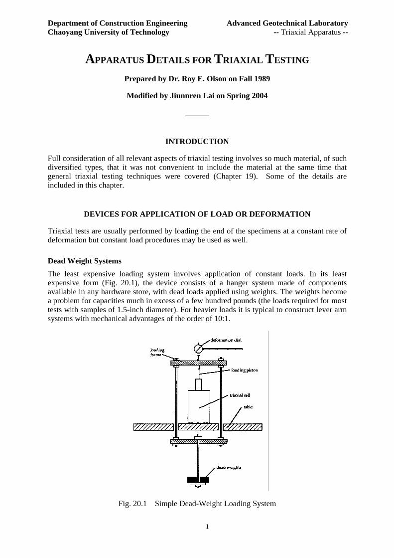
A hydraulic loading device can be mounted directly on top of the triaxial cell (Fig. 20.3), thus eliminating the need for a separate loading press. Rolling diaphragms and cylinders of appropriate sizes provide the ability to control axial forces with good accuracy. If a pneumatic system is used, the loading piston of the loading device is double ended and has no seal around the piston part but the clearance between the piston and the cylinder wall is small enough that the air leakage is small (air bearing), leading to an essentially frictionless loading system. If a rolling diaphragm is used (as in the hydraulic system of Fig. 20.3), the air consumption is quite low and the air source can be a suitable air tank that can be pressurized using a usual air compressor, or can be pumped up by hand or using the tiny compressors
Department of Construction Engineering Advanced Geotechnical Laboratory Chaoyang University of Technology -- Triaxial Apparatus --
3
available from hardware stores to pump up tires (capacities typically in excess of 100 psi), and driven from a car battery, thus allowing field use.
Fig. 20.3 Triaxial Cell with Associated Hydraulic Loading System (Mitchell, 1981)
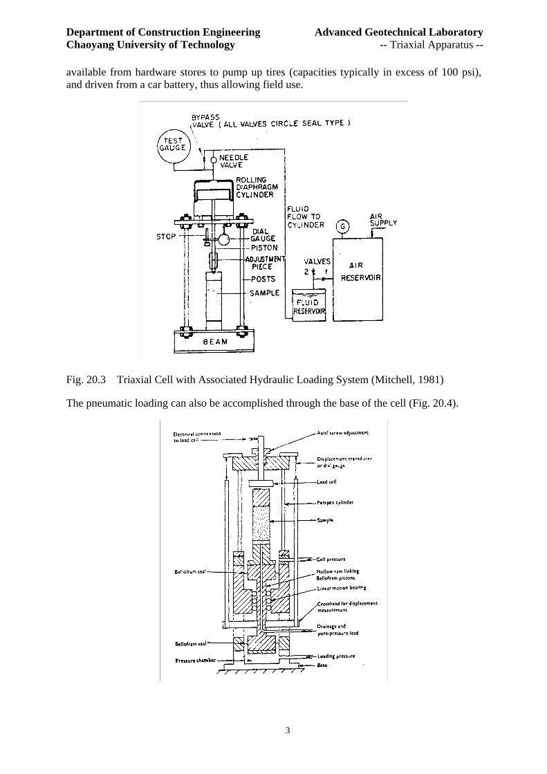
The pneumatic loading can also be accomplished through the base of the cell (Fig. 20.4).

Department of Construction Engineering Advanced Geotechnical Laboratory Chaoyang University of Technology -- Triaxial Apparatus --
4
Fig. 20.4 Triaxial Cell with Loading Applied Hydraulically Through the Base (Bishop and Wesley, 1981)
MEASUREMENT OF AXIAL DEFORMATION
Axial deformation of the sample in the triaxial apparatus is usually measured using a dial indicator or an electronic device (DCDT or LVDT) or both in combination. Combined dial indicators and DCDTs are often used to allow automatic recording of the data while still giving manual backup.
The usual procedure is to mount the dial indicator (that term will henceforth be used generically to include any deformation measuring device) on a frame which is either attached to the loading piston or the bottom of the load measuring device. With this arrangement, the dial indicator reads the change in height of the soil sample regardless of the compressibility of the load cell.
The main source of potential error in measuring total sample deformation is in the contact between the piston and the top cap (Fig. 20.5). During the consolidation stage in R and S tests, the sample may distort in such a way that the piston does not come down and bear concentrically on the insert. Thus/ during the initial stages of loading, the top cap displaces sideways slightly as the piston slides down into the insert. The problem is most easily remedied by applying a seating load sufficient to cause good bearing/ and then backing the load off, setting the deformation dial indicator to zero, and beginning the test. If the sample tends to distort significantly during the consolidation stage, then a guided attachment (Fig. 20.5c) may be needed.
Fig. 20.5 Various Design for Connection of Loading Piston and Top Cap
Department of Construction Engineering Advanced Geotechnical Laboratory Chaoyang University of Technology -- Triaxial Apparatus --
5
The average axial strain is defined to be the change in length of the sample divided by the length at the beginning of the shearing stage. Actual strains within the sample typically range widely, with the maximum strains at the center (Truesdale and Rusin, 1964) (see later discussion on end effects).
MEASUREMENT OF AXIAL FORCE
The axial force is usually measured using a proving ring or an electronic load cell. Measurements may be made externally or internally.
External Measurement of Loads
The usual procedure is to measure loads outside of the triaxial cell. The disadvantage of making external measurement of load is that there is friction between the loading piston and the seal (required to retain the cell fluid). The advantages of external measurement include:
1. the load measuring unit is only required during the shearing phase so the laboratory need buy only one load cell per press rather than one per triaxial cell
2. the load cell is readily accessible
3. problems with corrosion and shorting out of electric lines are generally negligible
Internal Measurement of Applied Axial Force
There remain cases where it is better to measure the load internally:
1. in cyclic shear tests, the error caused by piston friction is accentuated because the direction of the friction reverses when loading direction reverses
2. in dynamic tests, use of internal load cells can minimize problems in accounting for inertial effects
3. internal measurement may be convenient for creep tests where small variations in piston friction are important (with internal measurement/ the variation of applied load due to time-dependent variation in piston friction is known).
4. for some research testing where a high degree of accuracy is desired, internal measurement of load is preferred.
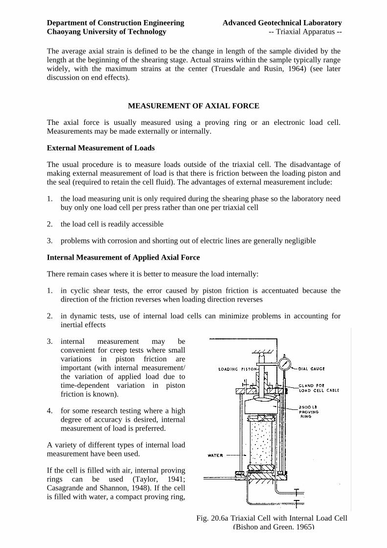
A variety of different types of internal load measurement have been used.
If the cell is filled with air, internal proving rings can be used (Taylor, 1941; Casagrande and Shannon, 1948). If the cell is filled with water, a compact proving ring,
Fig. 20.6a Triaxial Cell with Internal Load Cell (Bishop and Green, 1965)
Department of Construction Engineering Advanced Geotechnical Laboratory Chaoyang University of Technology -- Triaxial Apparatus --
6
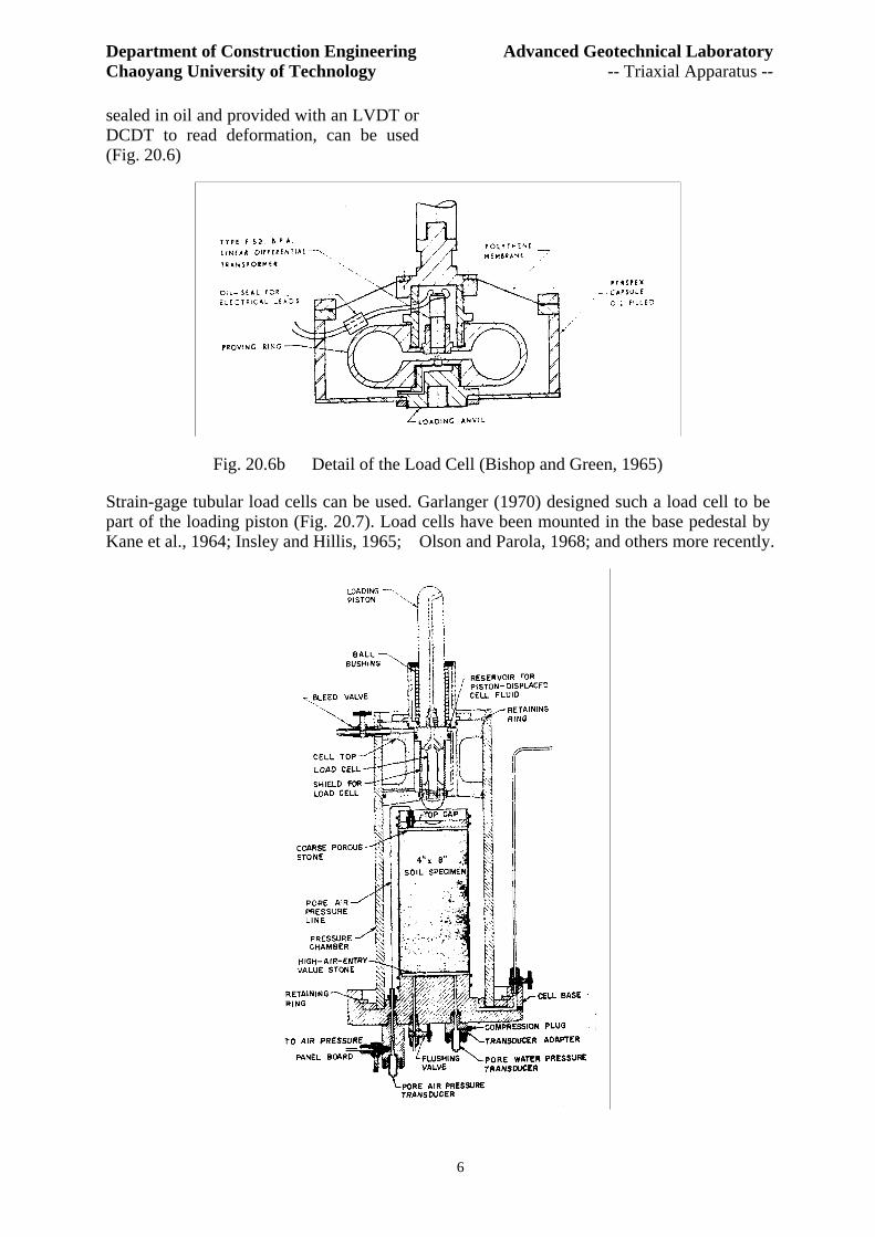
sealed in oil and provided with an LVDT or DCDT to read deformation, can be used (Fig. 20.6)
Fig. 20.6b Detail of the Load Cell (Bishop and Green, 1965)
Strain-gage tubular load cells can be used. Garlanger (1970) designed such a load cell to be part of the loading piston (Fig. 20.7). Load cells have been mounted in the base pedestal by Kane et al., 1964; Insley and Hillis, 1965; Olson and Parola, 1968; and others more recently.

Department of Construction Engineering Advanced Geotechnical Laboratory Chaoyang University of Technology -- Triaxial Apparatus --
7
Fig. 20.7 Triaxial Cell with Tubular Load cell Mounted Directly in the Loading Piston (Garlanger, 1970)
METHODS OF APPLYING CONFINING PRESSURE
The triaxial cell is filled with a fluid (liquid or gas) which is used to subject the sample to the confining pressure. Several fluids are used and there are a variety of ways of pressurizing the fluid.
Direct Gas Pressure When the cell fluid is gas, it is possible to pressurize the cell very quickly and the pressure may be maintained for any desired period of time using air regulator valves. Pressures up to about 175 psi can be obtained using relatively inexpensive, small capacity, air compressors. Higher pressures may be obtained using pneumatic intensifiers, or compressed nitrogen in bottles. For pressures under 125 psi, special instrumentation-grade, low flow, air regulator valves are available that have a slow built-in leak to prevent the diaphragm from closing and potentially sticking, thus ensuring a higher level of accuracy than can be obtained using standard air regulator values. For pressures of less than 125 psi, these special air regulator values can usually maintain pressures constant within about 0.1 to 0.5 psi even with significant changes in the source pressure and with slow changes in temperature.
If compressed air is already available, the remaining required apparatus costs less than for other methods of applying cell pressure. Further, the bushing where the loading piston passes through the top of the cell can be a low friction ball bushing with a loose 0-ring seal which will cause negligible friction. A small amount of air leakage through the seal is tolerated.
Unfortunately, gas leaks rapidly through the readily available rubber membranes (Article 20.8) and use of membranes that are heavy enough to retard air leakage by an acceptable amount typically cause an error in calculated axial stress because a significant part of the applied axial stress is taken by the membrane (Article 20.7).
In addition, the high compressibility of gases means that failure of the cell walls will result in an explosion with a probability of serious injury to personnel who are near the cell. Our experience is that the bursting pressures of the plastic cell walls with ID'S of about 4.5 inches, and 0.25-inch wall thickness, is generally in excess of 500 psi for new plastic but this capacity will drop as the plastic ages. Further, some shipments of the tubing apparently have internal stresses left from forming, and have burst at pressures as low as 150 psi.
As a result of these problems, direct gas pressure is rarely used for pressures exceeding about 50 psi (350 kPa) for triaxial cells with plastic side walls, nor for tests that last longer than perhaps half an hour.
Gas Pressure Over Water in the Cell A relatively simple variation of the direct gas pressure technique is to fill the cell up to within one quarter inch of the top with water and then apply gas pressure in that zone. Many of the advantages of direct gas pressure remain. The danger of serious damage from an explosion is reduced because of the smaller quantity of air in the cell. A wire mesh hood can be placed around the top of the cell for further protection, or the top of the plastic cell wall can be wrapped in fiber glass tape. Since the gas is not in direct contact with the membrane, gas
Department of Construction Engineering Advanced Geotechnical Laboratory Chaoyang University of Technology -- Triaxial Apparatus --
8
leakage must be by diffusion, which will normally require at least a day before it becomes apparent. This method is acceptable for use with Q-tests on saturated clays, or where volume change observations are not required.
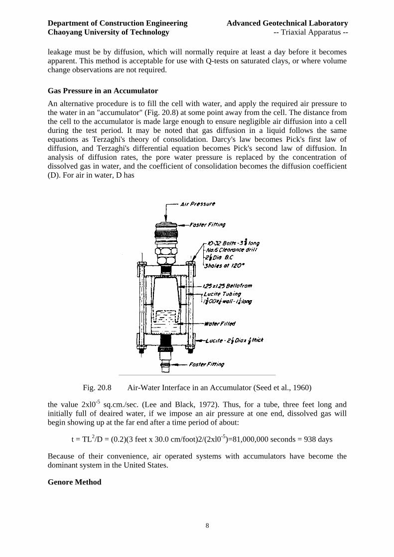
Gas Pressure in an Accumulator An alternative procedure is to fill the cell with water, and apply the required air pressure to the water in an "accumulator" (Fig. 20.8) at some point away from the cell. The distance from the cell to the accumulator is made large enough to ensure negligible air diffusion into a cell during the test period. It may be noted that gas diffusion in a liquid follows the same equations as Terzaghi's theory of consolidation. Darcy's law becomes Pick's first law of diffusion, and Terzaghi's differential equation becomes Pick's second law of diffusion. In analysis of diffusion rates, the pore water pressure is replaced by the concentration of dissolved gas in water, and the coefficient of consolidation becomes the diffusion coefficient (D). For air in water, D has
Fig. 20.8 Air-Water Interface in an Accumulator (Seed et al., 1960)
the value 2xl0-5 sq.cm./sec. (Lee and Black, 1972). Thus, for a tube, three feet long and initially full of deaired water, if we impose an air pressure at one end, dissolved gas will begin showing up at the far end after a time period of about:
t = TL2/D = (0.2)(3 feet x 30.0 cm/foot)2/(2xl0-5)=81,000,000 seconds = 938 days
Because of their convenience, air operated systems with accumulators have become the dominant system in the United States.
Genore Method
Department of Construction Engineering Advanced Geotechnical Laboratory Chaoyang University of Technology -- Triaxial Apparatus --
9
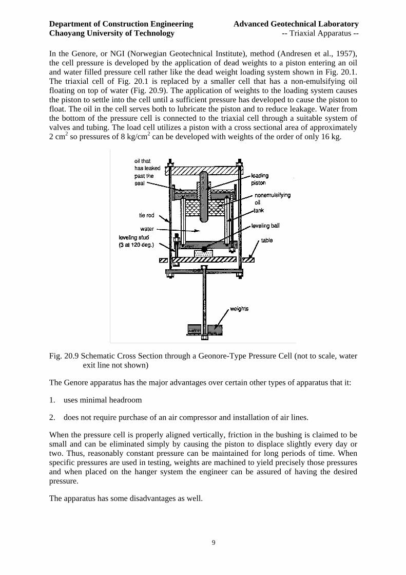
In the Genore, or NGI (Norwegian Geotechnical Institute), method (Andresen et al., 1957), the cell pressure is developed by the application of dead weights to a piston entering an oil and water filled pressure cell rather like the dead weight loading system shown in Fig. 20.1. The triaxial cell of Fig. 20.1 is replaced by a smaller cell that has a non-emulsifying oil floating on top of water (Fig. 20.9). The application of weights to the loading system causes the piston to settle into the cell until a sufficient pressure has developed to cause the piston to float. The oil in the cell serves both to lubricate the piston and to reduce leakage. Water from the bottom of the pressure cell is connected to the triaxial cell through a suitable system of valves and tubing. The load cell utilizes a piston with a cross sectional area of approximately 2 cm2 so pressures of 8 kg/cm2 can be developed with weights of the order of only 16 kg.
Fig. 20.9 Schematic Cross Section through a Geonore-Type Pressure Cell (not to scale, water exit line not shown)
The Genore apparatus has the major advantages over certain other types of apparatus that it:
1. uses minimal headroom
2. does not require purchase of an air compressor and installation of air lines.
When the pressure cell is properly aligned vertically, friction in the bushing is claimed to be small and can be eliminated simply by causing the piston to displace slightly every day or two. Thus, reasonably constant pressure can be maintained for long periods of time. When specific pressures are used in testing, weights are machined to yield precisely those pressures and when placed on the hanger system the engineer can be assured of having the desired pressure.
The apparatus has some disadvantages as well.

Department of Construction Engineering Advanced Geotechnical Laboratory Chaoyang University of Technology -- Triaxial Apparatus --
10
1. if compressed air lines are already available, it will usually be much cheaper to use an air operated system
2. the pressure cells have relatively small volumetric capacity so it is necessary to pump water back into them periodically to keep the piston from settling to the bottom of the cell
3. the oil slowly leaks past the bushing and collects in a special trough. Dust will often manage to get past the dust cover to make the oil gummy.
4. if a (readily available) lubricating oil is used, it will emulsify with the water and form a white gum which must then be cleaned out
5. this apparatus cannot be operated as quickly as the air operated equipment in setting up a test. This slowness is a disadvantage if a large number of Q tests are being performed with short testing times.
6. the apparatus only applies pressures for which loading weights exist.
7. significant amounts of piston friction can develop in the cell and lead to fluctuating output pressures.
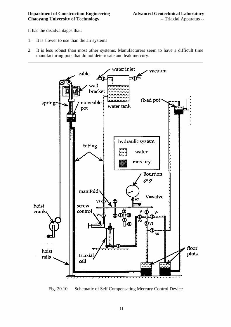
Imperial College Method At Imperial College, Bishop and Henkel (1953) developed the so-called “self compensating mercury control apparatus” (Fig. 20.10) for applying cell pressure. Pressure comes from a column of mercury. The unit weight of mercury is about 13.546 grams/ml at 20 deg. C. so the mercury pressure increases at a rate of about 5.87 psi per foot of elevation change. To achieve a variable pressure, mercury is contained in "pots" which are hung from springs. The pressure is developed by winching the pots up the wall on guide rails (Fig. 20.6) until the desired pressure is attained. The mercury from the pot being lifted is carried in a flexible tube down to the floor where it enters the bottom of a similar pot that serves as an accumulator. Water floats on the mercury in this pot. This pressurized water passes through another flexible tube to a panel board containing the needed valves and gages, and then to the triaxial cell (Fig. 20.10).
When a sample consolidates, a volume of mercury, equal to the change in volume of the sample, drains out of the moveable pot. This causes the pot to lose weight and causes the calibrated spring to lift the pot in such a way that the head remains constant. When all the mercury has run out of the moveable pot, the pot is refilled by reversing the direction of flow and pumping water back into the system.
For pressures higher than can be achieved with the head of mercury from the floor to the ceiling, additional pots are hooked in series. With twelve to fourteen foot ceilings, pressures of the order of 50-75 psi can be achieved for each floor-to-ceiling column of mercury.
The self-compensating mercury system has the advantages that:
1. It will maintain constant pressures for long periods of time,
2. It has minimal upkeep (compared to upkeep of air compressors, for example)
It can be used where compressed air is unavailable
Department of Construction Engineering Advanced Geotechnical Laboratory Chaoyang University of Technology -- Triaxial Apparatus --
11
It has the disadvantages that:
1. It is slower to use than the air systems
2. It is less robust than most other systems. Manufacturers seem to have a difficult time manufacturing pots that do not deteriorate and leak mercury.
Fig. 20.10 Schematic of Self Compensating Mercury Control Device
Department of Construction Engineering Advanced Geotechnical Laboratory Chaoyang University of Technology -- Triaxial Apparatus --
12
3. It requires considerable head room. In this regard, however, it may be noted that the apparatus has been used successfully for pressures as high as 1000 psi (Bishop, Webb, and Skinner, 1965)
4. Mercury is generally considered poisonous (we know of no evidence of problems with mercury provided that the laboratory is well ventilated and any spilled mercury is cleaned Up).
Systems for Higher Pressures Various types of pneumatic and hydraulic systems are in use for the development of pressures in the range from say 200 psi on up into the over 100,000 psi range. The apparatus for such testing is comparatively expensive and samples consolidated to such pressures should probably be considered rock (shale, sandstone, etc.) rather than soil so there is little need to discuss such apparatus in detail.
For soil testing purposes, systems using compressed nitrogen and an accumulator are convenient for pressures up to 1000 psi.
A hydraulic system in common use for such testing is a variation on the hydraulic tester for calibrating Bourdon gages, and is of the same general design as the NGI system (Art. 20.3.4). It consists of a small diameter steel piston sliding down a straight bushing. Static weights are applied to the top of the piston to develop the desired oil pressure beneath. The oil is connected to an accumulator which is usually a steel cylinder containing a rubber membrane which separates oil on one side from water on the other side. The water goes to the triaxial cell. The oil also goes to a hydraulic pump. When a force is applied to the piston, the piston settles quickly (the volume capacity of the apparatus is small) and a projection on the top of the piston strikes a limit switch which turns on the hydraulic pump. Oil is pumped into the system until the piston is raised to its upper limit of travel where it strikes another limit switch which turns off the pump. Oil that leaks around the piston is recirculated to the pump. The pump, tubing, and piston are designed in such a way as to be compatible with the volume change characteristics of the sample and triaxial cell. Thus, the cell can be pumped up to capacity in a reasonable period of time but the pump does not rapidly cycle on and off during the time that the cell pressure is being held constant.
Other systems utilize pneumatic or hydraulic intensifiers in which a large diameter piston is mechanically connected to a small diameter piston. The application of a pressure to the face of the large piston, as with compressed air or hydraulic pressure, produces a force equal to the product of the pressure and the area of the piston. This force is transmitted mechanically to the piston of smaller diameter. For equilibrium to occur the pressure developed in the fluid in contact with the piston of smaller area must be greater than the initially applied pressure to the larger piston, i.e., the pressure is intensified. When suitably equipped with limit switches, solenoid valves, and pressure transducers, the apparatus can be made to intensify normal line pressures of say 100 psi up into the very high pressure range.
DESIGN AND PERFORMANCE OF PISTON BUSHINGS
Because it is usually more economical to measure the load in the loading piston outside the cell, rather than inside, the friction of the bushing must be minimized. Simultaneously, the bushing must be tolerably leak proof, its construction must be economical, and it must allow adequate vertical movement of the piston. These requirements are partially in conflict so the
Department of Construction Engineering Advanced Geotechnical Laboratory Chaoyang University of Technology -- Triaxial Apparatus --
13
design actually used will represent a compromise. The proper compromise may depend on the type of test being performed, the amount of confining pressure, the duration of the test, the loading speed, and a variety of other factors. Rather than recommend a single solution to this problem it is better to survey the solutions available and let the individual engineer make the choice.
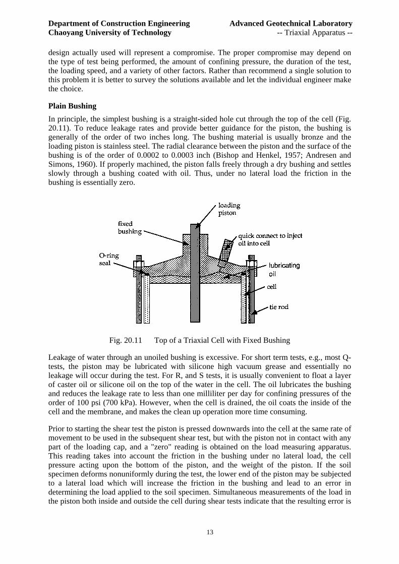
Plain Bushing In principle, the simplest bushing is a straight-sided hole cut through the top of the cell (Fig. 20.11). To reduce leakage rates and provide better guidance for the piston, the bushing is generally of the order of two inches long. The bushing material is usually bronze and the loading piston is stainless steel. The radial clearance between the piston and the surface of the bushing is of the order of 0.0002 to 0.0003 inch (Bishop and Henkel, 1957; Andresen and Simons, 1960). If properly machined, the piston falls freely through a dry bushing and settles slowly through a bushing coated with oil. Thus, under no lateral load the friction in the bushing is essentially zero.
Fig. 20.11 Top of a Triaxial Cell with Fixed Bushing
Leakage of water through an unoiled bushing is excessive. For short term tests, e.g., most Q-tests, the piston may be lubricated with silicone high vacuum grease and essentially no leakage will occur during the test. For R, and S tests, it is usually convenient to float a layer of caster oil or silicone oil on the top of the water in the cell. The oil lubricates the bushing and reduces the leakage rate to less than one milliliter per day for confining pressures of the order of 100 psi (700 kPa). However, when the cell is drained, the oil coats the inside of the cell and the membrane, and makes the clean up operation more time consuming.
Prior to starting the shear test the piston is pressed downwards into the cell at the same rate of movement to be used in the subsequent shear test, but with the piston not in contact with any part of the loading cap, and a "zero" reading is obtained on the load measuring apparatus. This reading takes into account the friction in the bushing under no lateral load, the cell pressure acting upon the bottom of the piston, and the weight of the piston. If the soil specimen deforms nonuniformly during the test, the lower end of the piston may be subjected to a lateral load which will increase the friction in the bushing and lead to an error in determining the load applied to the soil specimen. Simultaneous measurements of the load in the piston both inside and outside the cell during shear tests indicate that the resulting error is

Department of Construction Engineering Advanced Geotechnical Laboratory Chaoyang University of Technology -- Triaxial Apparatus --
14
usually less than three percent (Rutledge, 1947; Bishop and Henkel, 1957; and Insley and Hillis, 1965) and may be less than one percent.
However, if the soil specimen is eccentric or fails along a single sloping shear plane and axial forces are measured at strains much in excess of the failure strain, frictional errors up to five percent of the axial load were reported by Bishop and Henkel (1957), up to nine percent by Andresen and Simons (1960), five to twenty percent by Blight (1967), and up to thirty three percent by Bishop, Webb, and Skinner (1965). The triaxial apparatus is generally not well suited to post-failure measurements on samples that fail on a dominant shear plane so frictional errors in excess of 3% of the applied load are unlikely.
Rotating Bushings Warlam (1960) was the first to advocate reduction of this friction by inducing faster movement between the piston and the bushing. Warlam estimated that bushing rotation at a rate of about one rpm would reduce friction by about ten times. Similar dramatic reductions in friction have been reported by Andresen and Simons (1960), Bishop, Webb, and Skinner (1956), Blight (1967), and Olson and Campbell (1967). The reduced amount of friction in cells with rotating bushings is also suggested by measurement of the net friction as a function of an applied lateral load (Fig. 20.12).
Fig. 20.12 Results of Friction Tests with Various Bushing (Olson and Campbell/1967)
Commercial triaxial cells are available with rotating bushings. Unfortunately, the bushings are difficult to machine and increase the cost of the triaxial cell considerably. Furthermore, in constant load tests, the rotation of the bushing may apply a small reciprocating axial load to the soil sample (Olson and Campbell, 1967).
Ball Bushings
Department of Construction Engineering Advanced Geotechnical Laboratory Chaoyang University of Technology -- Triaxial Apparatus --
15
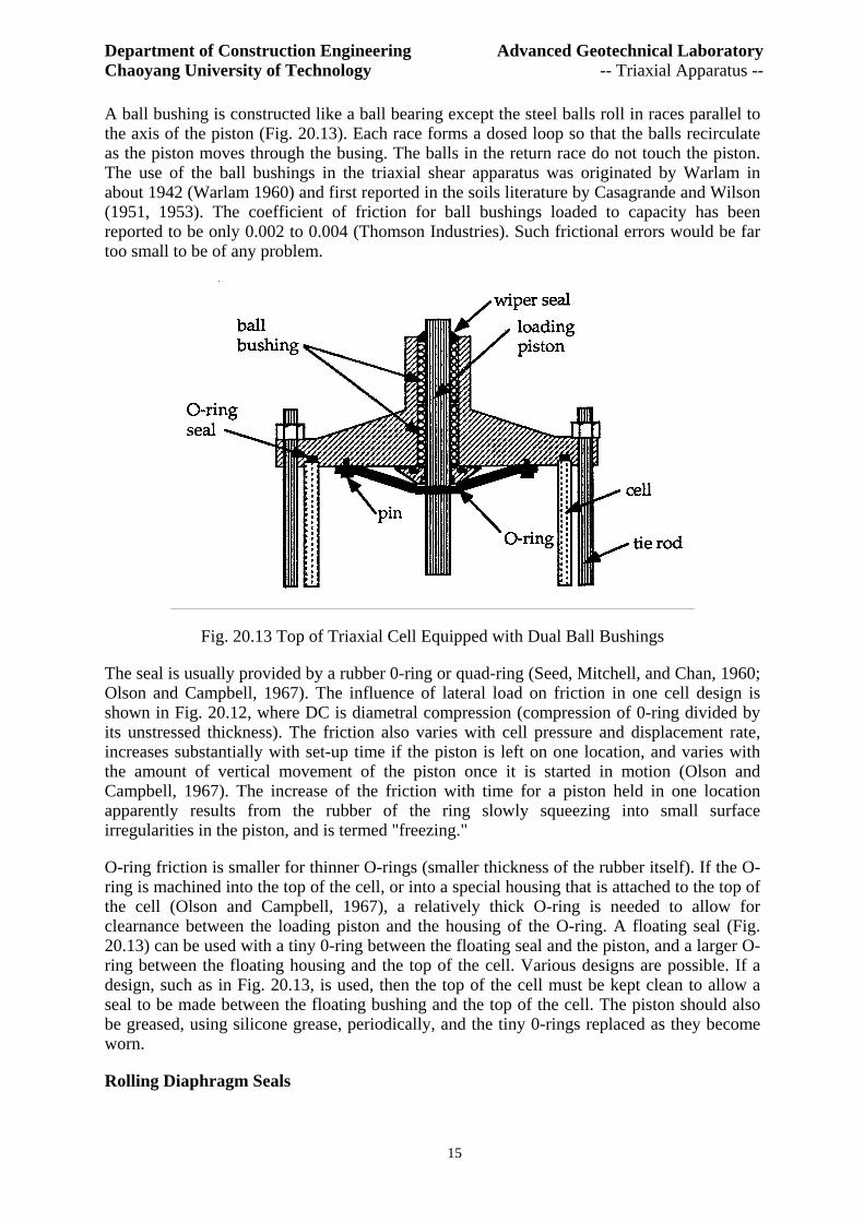
A ball bushing is constructed like a ball bearing except the steel balls roll in races parallel to the axis of the piston (Fig. 20.13). Each race forms a dosed loop so that the balls recirculate as the piston moves through the busing. The balls in the return race do not touch the piston. The use of the ball bushings in the triaxial shear apparatus was originated by Warlam in about 1942 (Warlam 1960) and first reported in the soils literature by Casagrande and Wilson (1951, 1953). The coefficient of friction for ball bushings loaded to capacity has been reported to be only 0.002 to 0.004 (Thomson Industries). Such frictional errors would be far too small to be of any problem.
Fig. 20.13 Top of Triaxial Cell Equipped with Dual Ball Bushings
The seal is usually provided by a rubber 0-ring or quad-ring (Seed, Mitchell, and Chan, 1960; Olson and Campbell, 1967). The influence of lateral load on friction in one cell design is shown in Fig. 20.12, where DC is diametral compression (compression of 0-ring divided by its unstressed thickness). The friction also varies with cell pressure and displacement rate, increases substantially with set-up time if the piston is left on one location, and varies with the amount of vertical movement of the piston once it is started in motion (Olson and Campbell, 1967). The increase of the friction with time for a piston held in one location apparently results from the rubber of the ring slowly squeezing into small surface irregularities in the piston, and is termed "freezing."
O-ring friction is smaller for thinner O-rings (smaller thickness of the rubber itself). If the O-ring is machined into the top of the cell, or into a special housing that is attached to the top of the cell (Olson and Campbell, 1967), a relatively thick O-ring is needed to allow for clearnance between the loading piston and the housing of the O-ring. A floating seal (Fig. 20.13) can be used with a tiny 0-ring between the floating seal and the piston, and a larger O- ring between the floating housing and the top of the cell. Various designs are possible. If a design, such as in Fig. 20.13, is used, then the top of the cell must be kept clean to allow a seal to be made between the floating bushing and the top of the cell. The piston should also be greased, using silicone grease, periodically, and the tiny 0-rings replaced as they become worn.
Rolling Diaphragm Seals

Department of Construction Engineering Advanced Geotechnical Laboratory Chaoyang University of Technology -- Triaxial Apparatus --
16
To reduce the seal-friction problem, Moore and Hirst (1970), and Campanella and Vaid (1972) designed a ball bushing seal in which a rolling diaphragm is used in place of the 0-ring seal, and the pressure differential across the diaphragm is reduced by injecting an air pressure (into the area above the seal) that is about 1~2 psi less than the cell pressure. The air pressure is allowed to leak out through the top of the bushing through a constriction that reduces the leakage rate to a tolerable limit without inducing friction. This bushing apparently works well but increases the cost of the bushing, provides a serious restriction on the allowable movement of the piston, and requires increased maintenance. For creep tests this bushing seems to be ideal.
Ball Bearing Bushing For tests with samples of large diameter it may be convenient to use a piston of large diameter and guide it with ball bearings. The piston would be supported at two levels and at each level there would be three ball bearings, each rotating on shafts perpendicular to the axis of the loading piston, with their outer races in contact with the loading piston (Warlam, 1960). With such a bushing/ the piston can be made of a softer and more light weight material, such as aluminum. A rolling diaphragm seal would be used to prevent leakage. Friction is minimized but problems may be encountered with the rolling diaphragm because of limited travel and development of leaks.
Pull-Down Loading An alternative loading scheme (reference) is to place a light cross-head above the sample, inside of the triaxial cell, with wires passing through glands in the top and bottom of the cell. Loading is accomplished by pulling on the wires. Frictional losses should be negligible because of the small size of the wires.
Conclusions At present, the most economical and convenient solution is to use ball bushings and a floating bushing. Frictional losses are minimal provided the loading piston is as small as possible and the smallest size O-ring is used in the floating bushing.
EFFECTS OF MEMBRANES AND DRAINS ON STRENGTH Membranes The soil sample is encased in a rubber membrane. As the sample is deformed the membrane is also deformed and probably takes an axial load itself as well as possibly changing the confining pressure.
In the first attempt to determine the influence of the rubber membrane on the strength of a clay in the triaxial apparatus (Rutledge, 1947) membranes with thicknesses of 0.015 and 0.025 inch were found to increase the apparent compressive strength of undisturbed day specimens by 160 psf and 540 psf, respectively.
Henkel and Gilbert (1952) studied the effects of membranes on the unconsolidated-undrained (Q) compressive strengths of 1.5-inch diameter samples of saturated, remolded clay. They found that the apparent increase in compressive strength of their samples did not depend on confining pressure (cell pressure), provided the cell pressure was greater than, or equal to, 5 psi. The apparent increases in compressive strengths were 45 psf, 85 psf, and 200 psf, for membranes with thicknesses of 0.004 inch, 0.008 inch, and 0.020 inch, respectively. Their samples failed at about 15% axial strain. Henkel and Gilbert offered some relatively

Department of Construction Engineering Advanced Geotechnical Laboratory Chaoyang University of Technology -- Triaxial Apparatus --
17
simplified equations for correcting both the stress difference and confining pressure.
The axial force carried by the membrane (Fma) can be estimated assuming the membrane does not buckle, in which case:
Fma = εErAr0η (20.1a)
where ε is axial compression of the sample measured from the time of set up (including the consolidation stage, if any), Er is Young's modulus for the rubber, Aro is the original sample area, and η is a factor.
200 4
DArπ
= (20.1b)
−−
−++−+−
=ευευσ
ευη
1111
11 3
rrE
(20.1c)
where ν is volumetric strain of the sample (positive for compression), ε is axial strain of the sample (positive for compression), σ3 is the cell pressure, and νr is Poisson's ratio of the rubber. If η=l, then Eq. 20.1a reduces to that for a linearly elastic, non-buckling, tube subject to small strains.
The expansion of the membrane during a shear test results in an increase in confining pressure ( ∆ σ3) of approximately:
ζσ0
03 2
DtEr=∆ (20.2a)
where
ευ
ευευσ
ευζ
−−
−−
−++−
−
−−
=
11
1111
111
3r
rE (20.2b)
The size of the error resulting from ignoring the presence of membranes clearly varies with the properties of the soil and the membranes. A few examples follow:
C psf
φ o
t in
Er psi
νr σ3 psi
ν %
ε %
∆ σ3 psi
ε(σ1-σ3)%
0 30 .002 400 0.33 20 10 20 0.1 1 0 30 .01 1000 0.33 20 10 20 0.8 11
250 0 .01 1000 0.33 20 0 20 0.8 122
where ε(σ1-σ3) represents the percentage error in the stress difference and other terms are as defined previously. Errors can be reduced to negligible proportions by selecting an appropriate membrane, or can become quite large if unreasonably heavy duty membranes are selected in order to make them last longer in the laboratory.
The foregoing equations yield results in general agreement with experimental measurements.

Department of Construction Engineering Advanced Geotechnical Laboratory Chaoyang University of Technology -- Triaxial Apparatus --
18
The correction to confining pressure should not be used when ∆ σ3 is negative (sample diameter is less than it was at set up time) because that would require that the membrane withstand a hoop stress in compression. The equations may not be reasonably correct if the membrane buckles.
In cases where the soil fails on a single dominant shear plane the mode of loading of the membrane changes after the shear plane forms. Tests by Chandler (1966) and Blight (1967) gave corrections that increased with both displacement and cell pressure. Corrections can be large. For example, Chandler's correction at a cell pressure of 100 psi and 0.5 inch of displacement (after the shearing plane forms), changed the apparent compressive strength of the sample by about 2000 psf. The triaxial device seems generally ill-suited to tests involving large deformations on single shear planes.
Filter Paper Drain Henkel and Gilbert (1952) repeated their Q-type compression tests on saturated samples using the 0.008-inch thick membrane but this time with a slotted Whatman No. 54 filter paper drain between the soil and the membrane. About 50% of the paper was removed in making the slots. After correcting for the strength of the membranes, they found that the filter paper increased the compressive strength of the specimens by about 200 psf. The magnitude of the correction was independent of the confining pressure.
For R and S tests, the filter paper consolidates along with the soil sample and the strength of the paper depends on the applied effective stresses (Olson and Kiefer, 1964). Paper-soil interaction is complex. Hard paper drains (Whatman No. 70) may actually buckle into the soil and reduce the apparent strength of the soil. For normally consolidated samples in R -type compression tests, Whatman No. 1 drains, with about half of the paper removed, increase Rφ by about 1.0 degree and CR by about 0.2psi.
To avoid questions about the compressive strength of the filter paper drain, some investigators use a strip of filter paper which is wrapped around the sample in spiral fashion, covering about half of the surface. The paper then goes into tension when the sample tries to expand and increases the confinement by some unknown amount. Further, the drainage path for water becomes long and it seems unreasonable to assume existence of a freely draining exterior boundary.
Corrections for other Types of Drains Acceleration of drainage has been achieved through use of internal sand drains and by the insertion of wool drains. No data are available on the effects of such drains on soil properties.
LEAKAGE THROUGH THE MEMBRANE, VALVES, AND FITTINGS
In analyzing the results of triaxial shear test, the assumption is usually made that the leakage through the membrane, and through the various valves and fittings is negligible. This assumption is not always valid and the engineer should be aware of when leakage can be a problem. The effects of leakage on measured soil properties will be briefly discussed and then observations of leakage will be summarized.
Effects of Leakage on Soil Properties During the consolidation stage, leakage leads to errors in the apparent volume change. For
Department of Construction Engineering Advanced Geotechnical Laboratory Chaoyang University of Technology -- Triaxial Apparatus --
19
samples undergoing compression during the consolidation stage, membrane leakage may cause the appearance of long-term secondary consolidation and lead to questions as to when the apparent consolidation has been completed. Diffusion of dissolved gas from the sample into deaired cell water gives the appearance of secondary consolidation with a negative slope (swelling).
In cases where the specimen is presumably sealed, leakage causes a volume change of the specimen and results in associated changes in the pore water pressure and effective stresses. Blight (1967) found that gas diffusion from a sealed sample resulted in increases in effective stress from 8 psi to 25 psi in one sample, and from 12 psi to 43 psi in another sample, both during a 48-hour period. Changes in effective stress cause changes in strength. If the soil is saturated and remains so during the time of leakage, and the total stress remains constant, then the change in pore water pressure ( ∆ u) and effective stress ( σ∆ ) in a specimen of specific gravity Gs, weight of solids Ws, and coefficient of compressibility "a", for a leakage of volume V, is simply given by:
aWVGu
s
ws ∆=∆−=∆
γσ (20.4)
where γw is the unit weight of water. More complicated formulas can be derived (Poulos, 1964) to cover other cases.
Leakage through the Rubber Membrane Direct gas leakage Direct measurements of gas leakage through rubber membranes were reported by Kane et al. (1964). For a sample covered with two membranes, each 0.002 inch thick, the leakage rate in cc per sec per sq.cm. varied from 9xl0-5 cm/sec at a gas pressure of 100 psi to 5xl0-4 cm/sec at 1000 psi. The volumes of gas were reported at atmospheric pressure.
As a first approximation, the effect of such leakage rates on the pore air pressure of a partially saturated specimen can be estimated by assuming that the gas in the void space obeys Boyle's law. As an example, if the specimen has a dry density of 117.4 pcf, a water content of 11.3 percent, and a specific gravity of solids of 2.72, and two membranes are used, during the early stages of leakage, the pore air pressure would change at a rate of 0.7 psi/min for the 100-psi confining pressure and 4.9 psi/min for the 1000-psi confining pressure. These pore air pressures act back against the inside of the rubber membranes and thus reduce the actual net confining pressure. The change in confining pressure, expressed as a percentage of the initial confining pressure, would be 0.7 and 0.5 percent/min at 100 psi and 1000 psi confining pressure, respectively. Such changes could be tolerated only in Q type tests where the shearing stage would follow the application of the confining pressure without significant delay.
For saturated samples, gas bubbles should start forming under the membrane soon after application of the confining pressure. Reduction in strength would occur as the gas dissolves in the pore water and raises the void ratio. For R and S tests the gas would cause anomalous volume change readings and would unsaturate the sample and the measuring system.
The leakage rate could be reduced by use of thicker rubber membranes but then a larger correction would be required for the strength of the membrane. It appears that direct gas loading can be used only for tests where the total time the sample is subjected to the gas pressure is short, generally less than say 30 minutes.
Department of Construction Engineering Advanced Geotechnical Laboratory Chaoyang University of Technology -- Triaxial Apparatus --
20
Gas diffusion leakage One way of retaining many of the advantages of gas loading, but with the gas separated from the membrane, is to fill the cell most of the way to the top with water and then apply gas pressure to the top of the water. The danger of a serious cell explosion is reduced by having only about 0.2-inch of gas in the cell, and the gas does not come into contact with the membrane. For a test with an air pressure of 75 psi applied at the top of a cell that was nearly filled with (initially) deaired water, steady state gas leakage developed after 3.5 days and, for a single membrane with a thickness of 0.002 inch, amounted to 1.5xl0-7 cm/sec (1.2 cc/day for a 1.5-inch diameter by 3.0-inch tall sample). Using a similar experimental arrangement, Seed, Mitchell, and Chan (1960) reported a steady state gas leakage rate of 2.2 cc/day for a pressure 15 psi (2.8x10⁻⁷ cm/sec).
Based on such experiments, it appears that test procedures in which the cell is filled almost to the top with water, and then air pressure is applied to this water, may be used for tests lasting up to about two to three days. This time might be extended somewhat if the cell fluid is initially completely deaired, if a heavier membrane is used, and for larger cells where the diffusion distance is increased, but serious leakage will usually occur before it is possible to complete normal R or S tests on clays. Such tests on sands and silts would probably be possible without significant error.
Water leakage through membranes Direct measurements of total water leakage were taken by setting up a saturated 1.5-inch diameter by 3.0-inch high porous stone, surrounding it with a filter paper drain and a single 0.002-inch thick membrane sealed top and bottom with two tight rubber 0-rings at each end, and measuring total water flow from the specimen. Once gas diffusion had stopped, the leakage rates were smaller than 0.01 ml/day for pressures up to 100 psi. Such leakage rates are too small to be of concern for routine triaxial testing but may be of concern for relatively incompressible samples.
Water leakage rates may be of concern for long-term tests with relatively incompressible soils. Poulos (1964) measured leakage through Ramses membranes (thickness 0.0024 inch). For water pressure drops between 2 and 11.5 kg/cm2 he found that the water flow through the membranes was in accord with Darcy's Law with the coefficient of hydraulic conductivity being about 4.8 x 10⁻¹⁶ cm/sec. ±35%. Soaking the membranes in silicone oil caused a small, but insignificant, decrease in leakage. For a sample 1.5-inches in diameter by 3.5-inches high, the calculated membrane leakage for a 100 psi pressure on a .002-inch thick membrane is 0.006 cc/day.
Leakage with Salt Solutions An experiment was performed (Olson, 1964b) to measure total leakage into a 1.5-inch diameter by 3.0-inch high porous stone but with the pore water of the stone containing l.0N CaCl2. The leakage rate was 0.090 ml/day. Application of a layer of high vacuum grease and another membrane reduced the leakage rate to 0.026 ml/day.
To show the effects of water leakage under a salt concentration gradient more clearly, another experiment was set up (Olson, 1964b) with a single membrane 0.002 inch thick and the 1.5-inch by 3.0-inch porous stone, and the stone was first saturated with 1N NaCl for a series of measurements and then it was flushed with distilled water until the effluent contained a salt concentration less than 1x10⁻⁴N and measurements were continued. The observations are shown in Table 1.
Table 1 Influence of Salt Concentration on Membrane Leakage
Confining Pressurepsi
Salt Concentration moles/liter
Measurement Time days
Leakage Rate ml/day

Department of Construction Engineering Advanced Geotechnical Laboratory Chaoyang University of Technology -- Triaxial Apparatus --
21
5 1 35 0.032 40 1 9 0.040 80 1 28 0.050 5 1 16 0.035 5 <0.0001 19 -0.001 40 <0.0001 40 0.006
Apparently, water diffuses through rubber membranes under a gradient in salt concentration as well as a pressure gradient. The salt concentration gradient can be converted, approximately, to an equivalent pressure gradient through an equation such as the van't Hoff equation:
CRT∆=π (20.5)
where ∆ C is the change in salt concentration from one side of the membrane to the other (moles per liter), R is the gas constant (liter atmospheres per degree mole), T is the absolute temperature (degree), and π is the osmotic pressure (atmospheres). For a difference in salt concentration of one mole per liter, the calculated osmotic pressure is about 360 psi. Apparently, leakage under osmotic gradients can be more important than pressure-gradient leakage for the pressures normally used in soil testing. Osmotic leakage can be prevented by establishing the same salt concentration on the two sides of the membrane. This will not generally be feasible for commercial testing but the foregoing leakage rates do not generally cause problems in commercial testing. The problems are more severe in special long-term tests; in these cases it may be necessary to perform chemical analyses to determine the pore water electrolyte concentration of the samples and establish the same chemistry in the cell fluid.
Gas leakage occurs in the opposite direction, i.e., from the sample into the water in the cell, when the cell water is initially deaired (Bishop, 1961a, Blight, 1967).
Leakage through the bindings Water or gas may presumably leak under the bindings for the triaxial membrane, as well as leaking directly through the membrane. Poulos (1964) measured binding leakage by using a 1.4-inch diameter by 0.1-inch high porous stone in place of the soil sample and measuring the combined leakage through both the membrane and the bindings. The membrane leakage was then calculated, using the data just discussed, and subtracted out. Since the membrane leakage exceeded the binding leakage and had a degree of uncertainty itself, the "measured" binding leakage was determined as the difference between two large numbers, and thus has a low degree of accuracy. However, since binding leakage turns out to be less than membrane leakage, a high degree of accuracy is not needed. The membranes were again Ramses. They were mounted on a rod 1.400 inches in diameter containing the porous stone. When 0-rings bindings were used, the 0-rings were Buna-N rubber of Shore A hardness 70, with unstretched dimensions of 0.984-inch I.D. and 1.262-inch O.D. Other tests were performed with the membranes bound to the rod using strips of neoprene rubber each of which was 0.2-inch wide, 1/32-inch thick, and 12 inches long. Six or seven wraps of the strip were used. The tests were performed with one binding (one 0-ring or one strip) on each side of the porous stone.
For a single membrane sealed against polished, ungreased stainless steel surfaces, the leakage rate was 0.00008 cc/day. When two membranes were used the leakage through the bindings increased to 0.0002 cc/day (but, of course, the leakage through the membrane was cut in half). It was not apparent why the leakage through the binding increased. Roughening the rod by
Department of Construction Engineering Advanced Geotechnical Laboratory Chaoyang University of Technology -- Triaxial Apparatus --
22
cutting grooves into it led to erratic results with generally more leakage. Coating the rod with high vacuum grease did not reduce leakage for the polished stainless steel and had no consistent effect for the roughened steel because of the large scatter. Use of grease was recommended in any case. Soaking the membranes in silicone oil did not reduce binding leakage. Use of the strips in place of the 0-rings led to erratic results because most of the strips were drawn so tightly that they failed during the tests. However, it appeared that there were several times as much leakage through the bindings made with strips as for those with O-rings.
Poulos's tests show that properly made bindings will leak much less than the membranes and thus should not be a problem, provided the cell fluid is water.
Rowe and Barden (1964) studied total leakage into a four-inch diameter by four-inch high soil specimen. A "commercial" membrane was used and it was sealed to the top cap and base using three 0-rings each. The leakage rate at a pressure of 10 psi was 0.050 cc/hr. After specially polishing the top and base and squeezing the 0-rings using a metal clamp, the leakage dropped to 0.0009 cc/hr for a confining pressure of 20 psi.
Leakage with Other Fluids Rowe and Barden (1964) found that leakage was about 0.050 cc/hr when glycerine was used as a cell fluid so they found no advantage in switching from water in the cell to glycerine.
Leakage through valves Poulos (1964) also measured leakage through valves of the types that might be used in pore pressure measuring systems. Generally his measured leakage rates varied widely. Scarring of the seat of needle valves, nicking 0-rings in plug and globe valves, and compression of packing in plug values, may lead to sudden and large amount of leakage whereas the valve in good condition may leak very little. Leakage rates ranged about as follows:
Table 2 Leakage through Valves (Poulos, 1964)
Valve and Situation Range in Leakage Rates (mm3/day) back against the seat of a needle value 0.001 to 0.01
eat and bonnet of needle valves 0.005 to 0.02 Circle Seal®, seat only 0.001 to 0.007
Circle Seal® (seat and bonnet) 0.2 to 0.3 Piston 0.1
Klinger® AB-10 0.02 to 200
In this table, "piston" valves have a piston, sealed with O-rings, that slides back and forth to open and close the valves.
Although the Klinger valves had the greatest amount of leakage, it should be noted that a visible leak in a Klinger valve can often be rectified by tightening on the packing nut whereas the sudden failure of an O-ring in some of the other valves requires dismantling of the valve.
Leakage rates of the order of 0.003 mm3/day probably occurred in some of the fittings so rates this small may actually correspond to no leakage. Rates smaller than about 0.01 mm3/day were difficult to measure and are probably not highly accurate. Such rates are so much smaller than the probable rates of leakage through the membranes that errors up to perhaps 50 percent are unimportant.
The compliance (change in volume per unit change in pressure) of the needle valves ranged

Department of Construction Engineering Advanced Geotechnical Laboratory Chaoyang University of Technology -- Triaxial Apparatus --
23
from 0.01 to 0.14 mm3/(kg/cm2) with no important difference between the two valves. The compliances of the plug, ball, and piston valves were generally comparable, ranging from 0.05 to 0.8 mm3/(kg/cm2) with the Klinger valve the least compressible and the Circle Seal valves having the most scatter in observations (0.04 to 0.48 mm2/kg/cm2).
END RESTRAINT
In the interpretation of the results of triaxial tests, it is convenient to assume that all horizontal and vertical planes are principal planes and that strains are uniform throughout the specimen. Based on these assumptions the applied axial force is easily converted into a stress and the axial strain can be calculated just by dividing the total measured displacement of the loading piston by the initial height of the specimen. Unfortunately, it is apparent, even to the eye, that stresses and strains must be nonuniform for axial strains much in excess of about five percent because the specimen either fails on a dominant shear plane or undergoes bulging in the middle. It is of interest to determine the effect that these nonuniformities have on measured soil properties and also to determine what methods are available for reducing the degree of nonuniformity.
Effect of Nonuniformities on Measured Compressive Strength If stress and strains were uniform in triaxial specimens, then the compressive strength would be independent of the height-to-diameter ratio (H/D). As an example of an early study, Casagrande (1940) reported a series of S-type compression tests on 1.4-inch diameter specimens of dry Franklin Falls sand. For one group of tests in which the initial void ratio was 0.71 and the confining pressure was 60 psi, the values of stress difference at failure were as follows:
H/D 1.0 1.5 2.5 3.0 (σ1- σ3), psi 36.6 22.2 21.0 21.6
Some specimens with H/D ratios of three failed by buckling and were not considered. Similar results have been reported by Kezdi (1957), Olson and Campbell (1964), Bishop and Green (1965), and others, for soils, and by other investigators for rock, concrete, metals, and other materials. The experimental data do not indicate a height-to-diameter ratio where end effects are eliminated but a ratio of 2.0 to 2.5 is commonly used on the grounds that use of slightly larger values does not reduce the strength significantly and use of much larger values leads to buckling.
Effective-Stress Shearing Properties
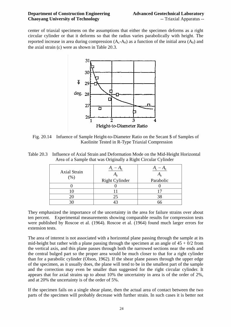
The tests on sand previously mentioned can also be interpreted in terms of φ and indicate a substantial reduction as H/D increases. The results of a series of S-type compression triaxial tests on specimens of a saturated kaolinite at different H/D ratios (Olson and Campbell, 1964) are shown in Fig. 20.14. They indicate a change in φ of the order of 10% for H/D ratios from 1.1 to 3.0. However, for values of H/D greater than about 1.6 the change in φ is little more than the scatter in the observations.
Calculation of the area of the specimen Roscoe, Schofield, and Wroth (1959) compared the calculated horizontal areas (Aε) at the
Department of Construction Engineering Advanced Geotechnical Laboratory Chaoyang University of Technology -- Triaxial Apparatus --
24
center of triaxial specimens on the assumptions that either the specimen deforms as a right circular cylinder or that it deforms so that the radius varies parabolically with height. The reported increase in area during compression (Aε-A0) as a function of the initial area (A0) and the axial strain (ε) were as shown in Table 20.3.
Fig. 20.14 Infuence of Sample Height-to-Diameter Ratio on the Secant $ of Samples of
Kaolinite Tested in R-Type Triaxial Compression
Table 20.3 Influence of Axial Strain and Deformation Mode on the Mid-Height Horizontal Area of a Sample that was Originally a Right Circular Cylinder
Axial Strain (%) 0
0
AAA −ε
Right Cylinder 0
0
AAA −ε
Parabolic 0 0 0 10 11 17 20 25 38 30 43 66
They emphasized the importance of the uncertainty in the area for failure strains over about ten percent. Experimental measurements showing comparable results for compression tests were published by Roscoe et al. (1964). Roscoe et al. (1964) found much larger errors for extension tests.
The area of interest is not associated with a horizontal plane passing through the sample at its mid-height but rather with a plane passing through the specimen at an angle of 45 + 0/2 from the vertical axis, and this plane passes through both the narrowed sections near the ends and the central bulged part so the proper area would be much closer to that for a right cylinder than for a parabolic cylinder (Olson, 1962). If the shear plane passes through the upper edge of the specimen, as it usually does, the plane will tend to be in the smallest part of the sample and the correction may even be smaller than suggested for the right circular cylinder. It appears that for axial strains up to about 10% the uncertainty in area is of the order of 2%, and at 20% the uncertainty is of the order of 5%.
If the specimen fails on a single shear plane, then the actual area of contact between the two parts of the specimen will probably decrease with further strain. In such cases it is better not
Department of Construction Engineering Advanced Geotechnical Laboratory Chaoyang University of Technology -- Triaxial Apparatus --
25
to attempt to define stresses and strains after the shear plane forms (the strain is obviously meaningless after a shear plane forms). Fortunately, the shear plane does not form until the moment the stress difference peaks and the failure strain is usually less than 10% so little error results in the calculated compressive stress.
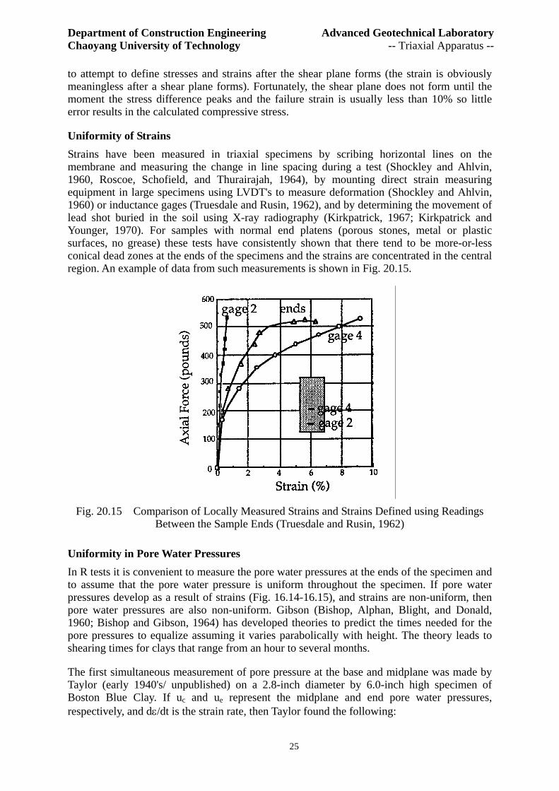
Uniformity of Strains Strains have been measured in triaxial specimens by scribing horizontal lines on the membrane and measuring the change in line spacing during a test (Shockley and Ahlvin, 1960, Roscoe, Schofield, and Thurairajah, 1964), by mounting direct strain measuring equipment in large specimens using LVDT's to measure deformation (Shockley and Ahlvin, 1960) or inductance gages (Truesdale and Rusin, 1962), and by determining the movement of lead shot buried in the soil using X-ray radiography (Kirkpatrick, 1967; Kirkpatrick and Younger, 1970). For samples with normal end platens (porous stones, metal or plastic surfaces, no grease) these tests have consistently shown that there tend to be more-or-less conical dead zones at the ends of the specimens and the strains are concentrated in the central region. An example of data from such measurements is shown in Fig. 20.15.
Fig. 20.15 Comparison of Locally Measured Strains and Strains Defined using Readings
Between the Sample Ends (Truesdale and Rusin, 1962)
Uniformity in Pore Water Pressures In R tests it is convenient to measure the pore water pressures at the ends of the specimen and to assume that the pore water pressure is uniform throughout the specimen. If pore water pressures develop as a result of strains (Fig. 16.14-16.15), and strains are non-uniform, then pore water pressures are also non-uniform. Gibson (Bishop, Alphan, Blight, and Donald, 1960; Bishop and Gibson, 1964) has developed theories to predict the times needed for the pore pressures to equalize assuming it varies parabolically with height. The theory leads to shearing times for clays that range from an hour to several months.
The first simultaneous measurement of pore pressure at the base and midplane was made by Taylor (early 1940's/ unpublished) on a 2.8-inch diameter by 6.0-inch high specimen of Boston Blue Clay. If uc and ue represent the midplane and end pore water pressures, respectively, and dε/dt is the strain rate, then Taylor found the following:
Department of Construction Engineering Advanced Geotechnical Laboratory Chaoyang University of Technology -- Triaxial Apparatus --
26
(uc-ue)/ uc (%) 30 19 0 dε/dt (%/min) 0.67 0.16 0.02
Subsequent measurements by Taylor and Clough (1951), Blight (1964, 1965), Barden and McDermott (1965), Garlanger (1970), and others, have shown that the midplane pore pressures exceed the pore pressures at the ends for normally consolidated days (and undoubtedly for loose sands) but are smaller for most overconsolidated clays and dense sands. For compacted clay, Bishop, Alpan, Blight and Donald (1960) found that the midplane pore pressures didn't necessarily even have the same sign as the end pore pressures, e.g./ in one 4-inch diameter by 8-inch high specimen of compacted shale at a compressive strain of 20% the midplane and end pore pressures were -3 psi and +9 psi, respectively, even though a period of 8 hours was used in deforming the sample to that strain.
Blight (1964) found that use of lubricated end plates reduced the nonuniformities in pore water pressures for compacted clay (p. 202) but had little effect for remolded clay (p. 204).
Uniformity in Water Content The variations in pore water pressure just discussed lead to hydraulic gradients and to water flow within specimens even for "undrained" samples in which the total volume is constant. The nonuniform water contents have been measured by Taylor and Clough (1951), Whitman, Ladd and de Cruz (1960), Crawford (1959, I960), Simons (1960a, 1960b), Olson (1960), Bishop, Blight, and Donald (I960), Rowe and Barden (1964), Barden and McDermott (1965), Casagrande and Poulos (1964) and others. Water content variations of over two percent have been reported.
Attempts to Eliminate End Effects From the foregoing discussion it is apparent that an effort should be made to reduce the end effects. Such an effort was started in the 1930's and continues to the present. Some of the methods tried and their success will be discussed below.
Segmented caps Kjellman (1936) and Taylor (1941) attempted to reduce end effects in a three-dimensional shear test and in the triaxial test, respectively, by segmenting the loading caps and then loading each segment separately through a rod. The method led to great complication in the apparatus but did not successfully eliminate end effects.
Curved caps For a specimen subject to uniform stresses, all horizontal and vertical planes are prindpal planes and all other planes are subjected to shear. If a cap could be designed with a curved contact surface with the soil specimen so that the shearing stresses on this curved surface were exactly the same as those in a specimen subject to uniform stresses, then presumably the specimen would deform uniformly. Attempts to use curved caps have been reported by Cooling and Golder (1940) and Larew (1960). The methods do not seem to have functioned well because the proper shape of the curved surface is different for different soils and may even vary with strain for a given soil. Further, it is not apparent how the trimming operation could be carried out.
Low-friction caps One way of ensuring that the ends of the specimens would be principal surfaces would be to load the specimen through "frictionless" surfaces. Although a truly frictionless surface does not exist it might be possible to eliminate a major part of the end effects with suitable low-friction surfaces. Note that end effects would not necessarily be eliminated even by perfectly frictionless ends because there would be an additional
Department of Construction Engineering Advanced Geotechnical Laboratory Chaoyang University of Technology -- Triaxial Apparatus --
27
requirement that the stress be uniform across the end.
One way of reducing the shearing stresses in the end surfaces would be to apply a thin rubber membrane to each end of the soil specimen, coat the rubber with a layer of oil or grease, and then load through a polished surface. The first reported use of this technique in shear testing of soils was by Roscoe (1953) for a plane strain device. Studies of the technique for triaxial testing were reported by Rowe and Barden (1964), Olson and Campbell (1964), Lee and Seed (1964), Bishop and Green (1965), Barden and McDermott (1965), and Duncan and Dunlop (1968). For testing of clays, these studies show that a single membrane about 0.002 inch thick, and a thin layer of silicone high vacuum grease will reduce the friction on the ends to about one degree. However, the grease acts as a viscous fluid and tends to extrude so that the friction angle builds up to values of two degrees or more within a period of three or four days. Such high friction values effectively constrain the ends so far as deformations are concerned. If the rubber-grease system is used, the surface of the cap and base should be polished but no reduction of friction results from using Teflon or a high polish.
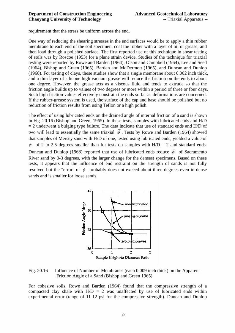
The effect of using lubricated ends on the drained angle of internal friction of a sand is shown in Fig. 20.16 (Bishop and Green, 1965). In these tests, samples with lubricated ends and H/D = 2 underwent a bulging type failure. The data indicate that use of standard ends and H/D of two will lead to essentially the same triaxial φ . Tests by Rowe and Barden (1964) showed that samples of Mersey sand with H/D of one, tested using lubricated ends, yielded a value of φ of 2 to 2.5 degrees smaller than for tests on samples with H/D = 2 and standard ends. Duncan and Dunlop (1968) reported that use of lubricated ends reduce φ of Sacramento River sand by 0-3 degrees, with the larger change for the densest specimens. Based on these tests, it appears that the influence of end restraint on the strength of sands is not fully resolved but the "error" of φ probably does not exceed about three degrees even in dense sands and is smaller for loose sands.
Fig. 20.16 Influence of Number of Membranes (each 0.009 inch thick) on the Apparent
Friction Angle of a Sand (Bishop and Green 1965)
For cohesive soils, Rowe and Barden (1964) found that the compressive strength of a compacted clay shale with H/D = 2 was unaffected by use of lubricated ends within experimental error (range of 11-12 psi for the compressive strength). Duncan and Dunlop

Department of Construction Engineering Advanced Geotechnical Laboratory Chaoyang University of Technology -- Triaxial Apparatus --
28
(1968) found decreases in compressive strength of the order of 0-8% when lubricated ends were used with clay but the effective angle of internal friction was reduced by only about one degree. Blight (1965) found that end lubrication had a negligible effect on the effective-stress failure envelope of clay.
Barden and McDermott (1965) and Blight (1965) both showed that use of lubricated ends leads to a great increase in the uniformity of the pore pressures within specimens of clay and thus to substantial reductions in testing times for R tests. They also found a tendency for the pore pressures in highly overconsolidated specimens to be more negative when lubricated ends were used, and to be higher for normally consolidated clays.
Ladanyi (1967) used an end transducer and found that stresses were peaked up in the center of the ends of samples even with lubricated end plates.
Discussion and Recommendations Regarding End Effects The available experimental data make it clear that when the standard triaxial testing procedures are used (high friction ends and H/D = 2) the strains in the specimens are nonuniform and result in bulging of the specimen, in nonuniform pore pressures, and to a small increase in the compressive strength. For most commercial testing, these "errors" are likely to be considerably smaller than errors associated with sampling disturbance, with use of nonrepresentative samples, with uncertainties in drainage conditions in the field, with use of incorrect or inaccurate theories, and with the various other problems that develop in practical foundation engineering. Further, the nonuniform pore pressures can be made reasonably uniform simply by reducing the deformation rate used during shear, and the slightly increased compressive strengths may help compensate for the fact that many field applications involve plane strain conditions and the plane-strain compressive strength is generally slightly higher than the triaxial compressive strength. Thus, the considerable increase in effort needed in setting up tests with lubricated ends does not seem to produce an equally large increase in the quality of the shear data, for practical applications. In the case of R and S tests, use of lubricated ends has a disadvantage in that the consolidation time is increased because of restrictions to the drainage surfaces.
For some research purposes, and for applications where the triaxial stress-strain properties are of interest, the use of lubricated ends may be justified. However, it must be remembered that present lubrication methods seem to become ineffective after a few days, because of extrusion of the grease, and that use of excessive lubrication may lead to changed failure modes, e.g., splitting of the specimen.
LOADING RATES FOR S-TYPE TRIAXIAL COMPRESSION TESTS S-type triaxial compression tests may be performed using either of two loading techniques, viz., the "constant load" and the "constant rate of deformation" techniques. Each has its own particular advantages and disadvantages and neither has received universal acceptance.
Constant Load Technique The constant load technique was discussed in Art. 20.1.2. If a simple hanger system is used to apply dead loads, the facts that the sample usually fails suddenly under the last load, and the inability to track any part of the stress-strain curve after failure, generally eliminates this testing mode. Use of hydraulic or pneumatic systems CH 20.2.3) may work better but these systems have not been widely used yet.

Department of Construction Engineering Advanced Geotechnical Laboratory Chaoyang University of Technology -- Triaxial Apparatus --
29
Of course, if creep testing under constant load is the goal, then the constant load procedure is used.
Constant-Rate-of-Deformation Technique The constant-rate-of-deformation procedure makes it possible to follow the stress-strain characteristics of the soil past failure, e.g., toward the "ultimate" condition and some engineers consider that it makes the collection of data simpler. Its disadvantages include more expensive apparatus and the fact that a deformation rate must be chosen from theory, or special experiments, to give an adequate degree of consolidation at failure. It is possible to use deformation rates that are too fast and not be aware of the resulting errors, e.g., measurement of excessively low strengths for normally consolidated soils and excessively high strengths for highly overconsolidated samples. Special consideration will now be given to the analysis of this deformation rate and to supporting experimental data.
The theory used to estimate the proper shearing time was developed by Gibson and Henkel (1954). In this theory, the soil is assumed to obey Biot's (1941) extension of Terzaghi's one-dimensional theory of consolidation. In Biot's theory the soil is assumed to be linearly elastic, as in Terzaghi's theory, but the deformations are three-dimensional. Darcy's law is assumed valid and water may flow in any direction. No secondary effects are taken into account. Since consolidation theory indicates that pore pressures generated by a loading never fully dissipate, it is necessary to calculate values for the degrees of consolidation at the moment of failure (Uf), as a function of time to failure, from theory and then to choose a suitable value for Uf, probably based on experimental measurements. The average degree of consolidation at failure is defined as:
R
PRf u
uuU −= (20.8)
where uR is the average excess pore water pressure in an undrained test at failure, and uP is the average excess pore water pressure in a partially drained test (an S test in which the pore pressures at failure do not go to zero throughout the specimen). The theory is needed to evaluate uR.
The details of the theory are not of interest here. The reader is referred to the papers by Gibson and Henkel (1954), Bishop and Gibson (1964), and Blight (1964) for the detailed equations and curves of degree of consolidation versus time factor. For large degrees of consolidation, as would normally be used in shear testing, the resulting equation is of the form:
f
f ctHU
η
2
1−= (20.10)
where H is half the height of the specimen (regardless of drainage conditions), η is a parameter to be tabulated, c is the coefficient of consolidation, and tf is the time from the start of shear to failure. Values for the parameter are as shown in Table 20.4.
The first two values apply regardless of the height-diameter ratio but the remaining values apply only to a height-diameter ratio of two. The drainage boundaries are assumed to be freely draining. The time-to-failure (tf) is calculated by rearranging Eq. 20.10 into the form:
Department of Construction Engineering Advanced Geotechnical Laboratory Chaoyang University of Technology -- Triaxial Apparatus --
30
)1(
2
ff Uc
Ht−
=η
(20.11)
Table 20.4 Drainage Factors for S Tests
drainage conditions η c
drainage from one end only 0.75 100
2
tHπ
rainage from both ends 3.0 100
2
4tHπ
radial drainage only 32.0 100
2
64tHπ
drainage radially and out both ends 40.4 100
2
100tHπ
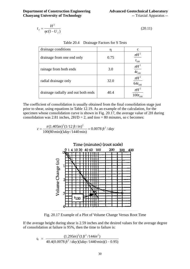
The coefficient of consolidation is usually obtained from the final consolidation stage just prior to shear, using equations in Table 12.19. As an example of the calculation, for the specimen whose consolidation curve is shown in Fig. 20.17, the average value of 2H during consolidation was 2.81 inches, 2H/D = 2, and tioo = 80 minutes, so c becomes:
dayftday
inftinc /0078.0min)1440/1min)(80(100)/12/1()405.1( 2
22
==π
Fig. 20.17 Example of a Plot of Volume Change Versus Root Time
If the average height during shear is 2.59 inches and the desired values for the average degree of consolidation at failure is 95%, then the time to failure is:
tf = )95.01min)(1440/1)(/0078.0(4.40
)144/1()295.1(2
222
−daydayftinftin

Department of Construction Engineering Advanced Geotechnical Laboratory Chaoyang University of Technology -- Triaxial Apparatus --
31
= 1064 minutes to failure
The deformation rate to be used in the S test is then obtained by estimating the deformation of the specimen at failure, adding in the deformation of load measuring equipment/ e.g., proving rings, and then dividing by the calculated time to failure.
In consideration of the approximations made in the development of the theory and in the selection of a degree of consolidation of 95%, it is convenient to develop a simpler and more approximate calculation for the time to failure. If it is assumed that the average height of the specimen during shear is approximately the same as during consolidation, then the equations from Table 20.4 can be inserted directly into Eq. 20.16 and the resulting equation simplified to contain only one variable, t100. For the two most common cases of all around drainage and drainage out one end only, the times to failure become 16 t100 and 8.5 t100, respectively.
Before a theory can be recommended for practical use it should be compared with suitable experimental data. The most direct way of checking on the validity of the Gibson-Henkel theory would be to measure the pore water pressures at several locations in specimens undergoing partially drained shear and to determine experimental values of Uf to compare with the theoretical values. However, the parameter of general interest is the shearing strength, not the residual pore pressures. For normally consolidated clays the S strength is of the order of twice the R strength so that the strength of specimens tested with open drains and increasing times to failure, should gradually increase to about twice the value obtained for very rapid tests and then the strength should remain nearly constant. Secondary corrections should be made for the fact that the strength of clays is a viscous phenomenon and varies with deformation rate even if the specimen is undrained.
Experimental studies of the influence of time-to-failure on the compressive strength were reported by Gibson and Henkel (1954) for a kaolinite with drainage out one end only, and for clays from Haslemere and London with all around drains; all specimens were remolded and saturated. Similar tests for sedimented specimens of illite are shown in Fig. 20.18. The tests all show that the compressive strength approximated the undrained strength for tests with small times to failure, rises as the testing time increases, peaks through most of a log cycle of time to failure, and then slowly decreases for longer times to failure, apparently because of viscosity of the soil structure. The theoretical degrees of consolidation are also shown in Fig.

Department of Construction Engineering Advanced Geotechnical Laboratory Chaoyang University of Technology -- Triaxial Apparatus --
32
Fig. 20.18 Influence of Time-to-Failure on the Compressive Strength of Normally Consolidated Samples of Illite
20.18. Apparently the peak strength occurs at about 95% consolidation but degrees of consolidation higher than about 90% yield essentially the same strength, within experimental scatter. Thus, if a specimen fails at a lower strain than estimated, and the calculated degree of consolidation at failure is slightly lower than 95%, it isn't necessary to perform another test.
However/ unpublished tests with kaolinite indicated that the compressive strength maximized at a time to failure about ten times smaller than predicted by the theory (see also Blight, 1964). The samples were provided with lateral filter paper drains and it was assumed that the drains were fully effective. Calculations, based on the assumption that the drains were ineffective led to a theoretical degree of consolidation at failure of about 95%.
A question thus arises about the effectiveness of lateral filter paper drains for some of the more pervious clays.
A large number of specimens of kaolinite were tested as part of a program to determine the influence of lateral filter paper drains on the compressive strength in undrained shear tests (Olson and Kiefer, 1963).
Coefficients of consolidation were calculated for specimens of normally consolidated kaolinite tested without drains, and with the normal slotted filter paper drains of Whatman No. 1 and No. 50 paper. Fitted coefficients of consolidation (Fig. 20.19) for samples without drains were near 0.01 sq.cm./sec. When samples were consolidated with lateral drains, the fitted coefficients of consolidation were about fifty times lower (Fig. 20.19). The most logical explanation of these observations was that the paper was not draining freely. If the paper drains were considered impervious, the fitted coefficients of consolidation were about two times too high (Fig. 20.19) so the paper apparently provided a limited amount of drainage. Bishop and Gibson (1964) reported some direct permeability measurements on filter paper (probably Whatman No. 54), subject to the error that they could not correct for the changing thickness of the paper as a function of the applied pressure. Their data are shown In Table 20.3.

Department of Construction Engineering Advanced Geotechnical Laboratory Chaoyang University of Technology -- Triaxial Apparatus --
33
Fig. 20.19 Calculated Coefficients of Consolidation for Samples of Normally Consolidated Kaolinite With and Without Lateral Filter Paper Drains
Table 20.3 Measured Hydraulic Conductivities of Filter Paper (Bishop and Gibson/ 1964)
Confining Pressure psi
Hydraulic Conductivity cm/sec.
4.5 1.7x10⁻³ 10 8.7x10⁻⁴ 30 3.2x10⁻⁴ 100 5.4x10⁻⁵ 300 1.1x10⁻⁵ 950 1.0x10⁻⁶
Considering the relatively small thickness of the filter paper, it is apparent that the paper will not be freely draining for many clays and nearly all silts. Blight (1964) tested a series of soils, with and without drains, and assumed that the coefficients of consolidation determined without drains were correct. He defined the efficiency of the drains as the ratio of the coefficients of consolidation for the tests with drains to those without. His efficiencies ranged from 15% to 77%. By way of comparison/ the efficiency of the filter paper drains used for the tests on kaolinite (Olson and Kiefer/1964) averaged about 1.5%.
Although lack of free drainage through the lateral filter paper drains will lead to substantial errors (up to 100 times) in the fitted coefficient of consolidation, the error largely cancels out when the incorrect coefficient of consolidation is inserted into the equation for calculating the time to failure. Thus, if the paper is assumed completely freely draining, the time to failure is 15.75 t100. If the paper was actually impervious the time to failure should have been 8.48 t100, where the t100 values are both the values actually obtained, regardless of the degree of drainage of the paper. Thus, if the engineer assumed the drains were fully effective, when in fact they were fully ineffective, the shearing time would be overestimated by a factor of 15.75/8.48 = 1.86 times. Such an error would increase testing costs somewhat but would not lead to a significant "error" in the measurement of the S strength.
Bishop and Gibson (1964) have analyzed the cases of partially draining ends, partially draining filter paper drains, and discontinuous lateral drains, and have provided analytical solutions for the calculation of the correct coeffident of consolidation and for calculation of the time to failure in terms of the correct coefficient of consolidation. Their conclusions are in line with the conclusions discussed above.
In the case of S tests on overconsolidated specimens, the S strength varies from about twice the R strength for overconsolidation ratios near one to about half the R strength for high overconsolidation ratios. No tests on the influence of time-to-failure on the compressive strength of overconsolidated specimens appear to be available/ but there is unlikely to be a distinct point, or even range, in times to failure where the specimens can be said to be drained, because for specimens with small overconsolidation ratios the R and S strengths are close together, and for highly overconsolidated specimens, the rate of reduction in strength as the specimen drains will merge with the rate of reduction due to soil viscosity, (run some tests on this point)
For highly overconsolidated specimens, failure tends to occur in thin zones in the specimen, because the zones where shearing strains initially concentrate lose strength after failure whereas adjacent areas that had not quite failed do not suffer such a loss in strength. The
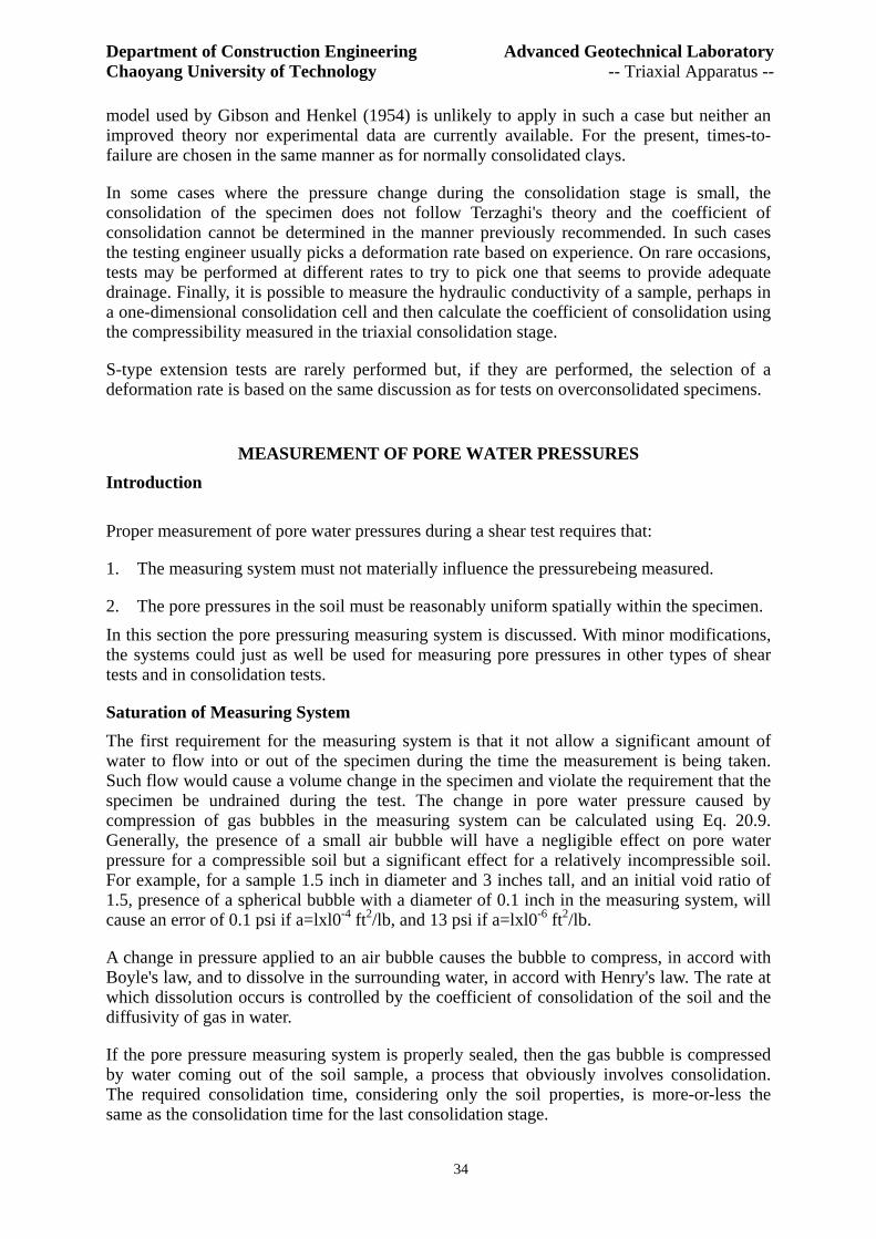
Department of Construction Engineering Advanced Geotechnical Laboratory Chaoyang University of Technology -- Triaxial Apparatus --
34
model used by Gibson and Henkel (1954) is unlikely to apply in such a case but neither an improved theory nor experimental data are currently available. For the present, times-to-failure are chosen in the same manner as for normally consolidated clays.
In some cases where the pressure change during the consolidation stage is small, the consolidation of the specimen does not follow Terzaghi's theory and the coefficient of consolidation cannot be determined in the manner previously recommended. In such cases the testing engineer usually picks a deformation rate based on experience. On rare occasions, tests may be performed at different rates to try to pick one that seems to provide adequate drainage. Finally, it is possible to measure the hydraulic conductivity of a sample, perhaps in a one-dimensional consolidation cell and then calculate the coefficient of consolidation using the compressibility measured in the triaxial consolidation stage.
S-type extension tests are rarely performed but, if they are performed, the selection of a deformation rate is based on the same discussion as for tests on overconsolidated specimens.
MEASUREMENT OF PORE WATER PRESSURES Introduction Proper measurement of pore water pressures during a shear test requires that:
1. The measuring system must not materially influence the pressurebeing measured.
2. The pore pressures in the soil must be reasonably uniform spatially within the specimen. In this section the pore pressuring measuring system is discussed. With minor modifications, the systems could just as well be used for measuring pore pressures in other types of shear tests and in consolidation tests.
Saturation of Measuring System The first requirement for the measuring system is that it not allow a significant amount of water to flow into or out of the specimen during the time the measurement is being taken. Such flow would cause a volume change in the specimen and violate the requirement that the specimen be undrained during the test. The change in pore water pressure caused by compression of gas bubbles in the measuring system can be calculated using Eq. 20.9. Generally, the presence of a small air bubble will have a negligible effect on pore water pressure for a compressible soil but a significant effect for a relatively incompressible soil. For example, for a sample 1.5 inch in diameter and 3 inches tall, and an initial void ratio of 1.5, presence of a spherical bubble with a diameter of 0.1 inch in the measuring system, will cause an error of 0.1 psi if a=lxl0-4 ft2/lb, and 13 psi if a=lxl0-6 ft2/lb.
A change in pressure applied to an air bubble causes the bubble to compress, in accord with Boyle's law, and to dissolve in the surrounding water, in accord with Henry's law. The rate at which dissolution occurs is controlled by the coefficient of consolidation of the soil and the diffusivity of gas in water.
If the pore pressure measuring system is properly sealed, then the gas bubble is compressed by water coming out of the soil sample, a process that obviously involves consolidation. The required consolidation time, considering only the soil properties, is more-or-less the same as the consolidation time for the last consolidation stage.
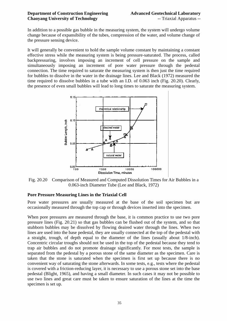
Department of Construction Engineering Advanced Geotechnical Laboratory Chaoyang University of Technology -- Triaxial Apparatus --
35
In addition to a possible gas bubble in the measuring system, the system will undergo volume change because of expansibility of the tubes, compression of the water, and volume change of the pressure sensing device.
It will generally be convenient to hold the sample volume constant by maintaining a constant effective stress while the measuring system is being pressure-saturated. The process, called backpressuring, involves imposing an increment of cell pressure on the sample and simultaneously imposing an increment of pore water pressure through the pedestal connection. The time required to saturate the measuring system is then just the time required for bubbles to dissolve in the water in the drainage lines. Lee and Black (1972) measured the time required to dissolve bubbles in a tube with an I.D. of 0.063 inch (Fig. 20.20). Clearly, the presence of even small bubbles will lead to long times to saturate the measuring system.
Fig. 20.20 Comparison of Measured and Computed Dissolution Times for Air Bubbles in a
0.063-inch Diameter Tube (Lee and Black, 1972)
Pore Pressure Measuring Lines in the Triaxial Cell Pore water pressures are usually measured at the base of the soil specimen but are occasionally measured through the top cap or through devices inserted into the specimen.
When pore pressures are measured through the base, it is common practice to use two pore pressure lines (Fig. 20.21) so that gas bubbles can be flushed out of the system, and so that stubborn bubbles may be dissolved by flowing deaired water through the lines. When two lines are used into the base pedestal, they are usually connected at the top of the pedestal with a straight, trough, of depth equal to the diameter of the lines (usually about 1/8-inch). Concentric circular troughs should not be used in the top of the pedestal because they tend to trap air bubbles and do not promote drainage significantly. For most tests, the sample is separated from the pedestal by a porous stone of the same diameter as the specimen. Care is taken that the stone is saturated when the specimen is first set up because there is no convenient way of saturating the stone afterwards. In some tests, e.g., tests where the pedestal is covered with a friction-reducing layer, it is necessary to use a porous stone set into the base pedestal (Blight, 1965), and having a small diameter. In such cases it may not be possible to use two lines and great care must be taken to ensure saturation of the lines at the time the specimen is set up.
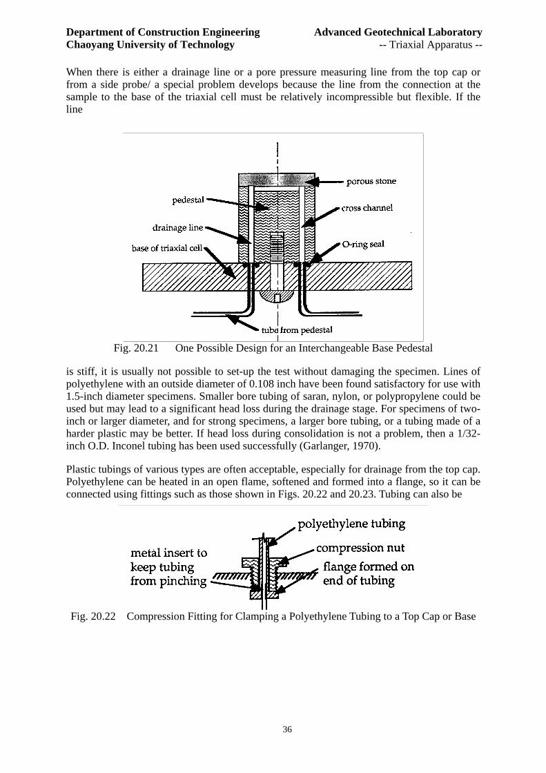
Department of Construction Engineering Advanced Geotechnical Laboratory Chaoyang University of Technology -- Triaxial Apparatus --
36
When there is either a drainage line or a pore pressure measuring line from the top cap or from a side probe/ a special problem develops because the line from the connection at the sample to the base of the triaxial cell must be relatively incompressible but flexible. If the line
Fig. 20.21 One Possible Design for an Interchangeable Base Pedestal
is stiff, it is usually not possible to set-up the test without damaging the specimen. Lines of polyethylene with an outside diameter of 0.108 inch have been found satisfactory for use with 1.5-inch diameter specimens. Smaller bore tubing of saran, nylon, or polypropylene could be used but may lead to a significant head loss during the drainage stage. For specimens of two-inch or larger diameter, and for strong specimens, a larger bore tubing, or a tubing made of a harder plastic may be better. If head loss during consolidation is not a problem, then a 1/32-inch O.D. Inconel tubing has been used successfully (Garlanger, 1970).
Plastic tubings of various types are often acceptable, especially for drainage from the top cap. Polyethylene can be heated in an open flame, softened and formed into a flange, so it can be connected using fittings such as those shown in Figs. 20.22 and 20.23. Tubing can also be
Fig. 20.22 Compression Fitting for Clamping a Polyethylene Tubing to a Top Cap or Base
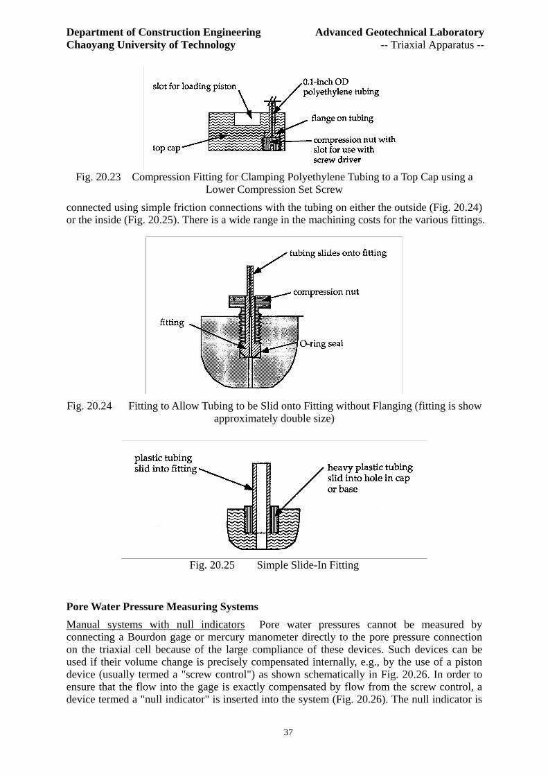
Department of Construction Engineering Advanced Geotechnical Laboratory Chaoyang University of Technology -- Triaxial Apparatus --
37
Fig. 20.23 Compression Fitting for Clamping Polyethylene Tubing to a Top Cap using a
Lower Compression Set Screw connected using simple friction connections with the tubing on either the outside (Fig. 20.24) or the inside (Fig. 20.25). There is a wide range in the machining costs for the various fittings.
Fig. 20.24 Fitting to Allow Tubing to be Slid onto Fitting without Flanging (fitting is show
approximately double size)
Fig. 20.25 Simple Slide-In Fitting
Pore Water Pressure Measuring Systems Manual systems with null indicators Pore water pressures cannot be measured by connecting a Bourdon gage or mercury manometer directly to the pore pressure connection on the triaxial cell because of the large compliance of these devices. Such devices can be used if their volume change is precisely compensated internally, e.g., by the use of a piston device (usually termed a "screw control") as shown schematically in Fig. 20.26. In order to ensure that the flow into the gage is exactly compensated by flow from the screw control, a device termed a "null indicator" is inserted into the system (Fig. 20.26). The null indicator is

Department of Construction Engineering Advanced Geotechnical Laboratory Chaoyang University of Technology -- Triaxial Apparatus --
38
a sensitive device for measuring movement of water in the line. The screw control is operated manually in such a way that there is no flow of water to or from the soil specimen, and the pressure is read on the gage. Manual systems are rarely used now because of the high labor cost involved in continual adjustment of the screw control.
Electrical pressure transducer Perhaps the simplest system/ mechanically, for measurement of pore water pressure is to use an electrical pressure transducer mounted directly on the base of the triaxial cell. Most pressure transducers in current use have a 1/8" NPT connection. The user selects an appropriate male tubing connector with a 1/8" NPT on one end and a tubing connector on the other end. The tubing is usually brass or stainless steel and is strong enough to provide support for the transducer.
Fig. 20.26 Schematic of Manual Pore Prerssure Measuring System
When the pore water pressure acts on the diaphragm of the transducer, it causes a small deflection of the diaphragm and strains the sensing element in the transducer. The sensing element may be a bonded or unbonded strain gage, or it may be an inductance gage. The transducer is calibrated against known pressures and a curve of the electrical parameter that is measured versus known pressure, is prepared.
The volume change of this system consists of the volume change of the water in the lines, volume change of the metal fittings, and volume change caused by deflection of the diaphragm of the transducer. The volume change of the water may be calculated from its bulk modulus, which is about 3.4x10⁻⁶ 1/psi. The volume of a typical measuring system is of the order of 0.1 in3. Thus, development of a pore water pressure of 100 psi would cause a volume change of about 3x10⁻⁵ in3. The compliance of a then widely used pressure transducer was measured at 4x10⁻⁷ in3/psi (Healy, 1960; Whitman, Richardson, Healy, 1961). Thus, for a 100-psi change in pressure, the transducer would undergo a volume change of about 4x10⁻⁵ in3. For a line drilled in metal, the volume change of the metal would probably be less than this amount. The total volume change would then probably be less than 10x10-5 in3. The resulting error in pore pressure, caused by this drainage, is given by Eq. 20.9 ( ∆ u=
σ∆− because σ∆ =0). For a 1.5-inch diameter by 3.0-inch high specimen, the resulting error in pore pressure is of the order of 10-6 psi, which is apparently much too small to be of concern.
Department of Construction Engineering Advanced Geotechnical Laboratory Chaoyang University of Technology -- Triaxial Apparatus --
39
The electrical transducer system has the advantages of great convenience over all other systems. If the output of the transducer is read on a digital volt meter it is usually possible to set the gain on the amplifier so that the reading on the voltmeter is equal to the pressure, in any convenient set of units.
TESTING RATES WHEN PORE WATER PRESSURES ARE TO BE MEASURED
In the earlier discussion of end effects, data were presented which showed that substantial gradients could be developed in the pore water pressures within soil specimens during undrained triaxial compression. If pore water pressures are to be measured through the base, then the loading rate must be sufficiently small so that the pore pressures can equalize throughout the specimen. It is possible to take measurements of the pore water pressure at mid-height of the specimen, though only with a considerable increase in the complexity of the apparatus, but if the pore pressures are nonuniform the mid-plane pore pressures are of little more use than the end values. Pore pressure gradients can be reduced, as discussed earlier, through the use of lubricated ends but this procedure complicates testing and has not received general acceptance for testing of cohesive soils for practical (non-research) purposes.
The actual phenomena occurring within a soil specimen during an undrained triaxial compression test are too complicated to be analyzed rigorously. Thus, it is preferable to derive an approximate theory and to check it against measurement, and then modify the approximate theory only to the extent necessary to bring it into conformance with the measurements. Gibson (Bishop, Alpan, Blight, and Donald, 1960) derived a theory to predict the rate of equilization of pore pressures in an undrained test based on the following assumptions:
1. Darcy's Law is valid
2. Soil properties are reasonably constant during shear
3. The soil is saturated
4. The coefficient of consolidation is the same for swelling as for consolidation
5. The excess pore water pressures vary parabolically in the vertical direction through the specimen but are independent of the radial distance
6. The radial boundary and the end boundaries are all impervious during shear
7. The rate of application of axial pressure is constant up to the point of failure
8. The pore pressure generated by an increment of axial pressure is a constant times that increment of pressure (the constant varies with vertical position in the specimen).
The degree of equilization of pore pressure was defined as follows (Blight, 1964):
0)(
)(1ce
tce
uuuuU
−−
−= (20.12)
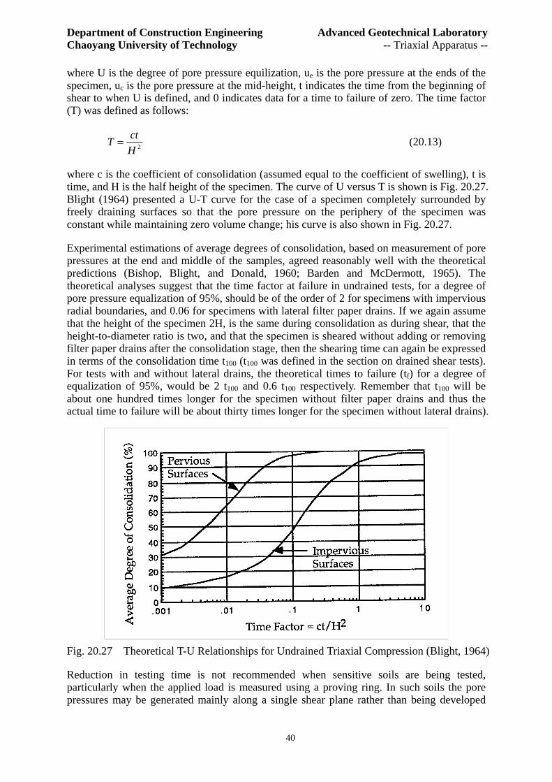
Department of Construction Engineering Advanced Geotechnical Laboratory Chaoyang University of Technology -- Triaxial Apparatus --
40
where U is the degree of pore pressure equilization, ue is the pore pressure at the ends of the specimen, uc is the pore pressure at the mid-height, t indicates the time from the beginning of shear to when U is defined, and 0 indicates data for a time to failure of zero. The time factor (T) was defined as follows:
2HctT = (20.13)
where c is the coefficient of consolidation (assumed equal to the coefficient of swelling), t is time, and H is the half height of the specimen. The curve of U versus T is shown is Fig. 20.27. Blight (1964) presented a U-T curve for the case of a specimen completely surrounded by freely draining surfaces so that the pore pressure on the periphery of the specimen was constant while maintaining zero volume change; his curve is also shown in Fig. 20.27.
Experimental estimations of average degrees of consolidation, based on measurement of pore pressures at the end and middle of the samples, agreed reasonably well with the theoretical predictions (Bishop, Blight, and Donald, 1960; Barden and McDermott, 1965). The theoretical analyses suggest that the time factor at failure in undrained tests, for a degree of pore pressure equalization of 95%, should be of the order of 2 for specimens with impervious radial boundaries, and 0.06 for specimens with lateral filter paper drains. If we again assume that the height of the specimen 2H, is the same during consolidation as during shear, that the height-to-diameter ratio is two, and that the specimen is sheared without adding or removing filter paper drains after the consolidation stage, then the shearing time can again be expressed in terms of the consolidation time t100 (t100 was defined in the section on drained shear tests). For tests with and without lateral drains, the theoretical times to failure (tf) for a degree of equalization of 95%, would be 2 t100 and 0.6 t100 respectively. Remember that t100 will be about one hundred times longer for the specimen without filter paper drains and thus the actual time to failure will be about thirty times longer for the specimen without lateral drains).
Fig. 20.27 Theoretical T-U Relationships for Undrained Triaxial Compression (Blight, 1964)
Reduction in testing time is not recommended when sensitive soils are being tested, particularly when the applied load is measured using a proving ring. In such soils the pore pressures may be generated mainly along a single shear plane rather than being developed
Department of Construction Engineering Advanced Geotechnical Laboratory Chaoyang University of Technology -- Triaxial Apparatus --
41
throughout large zones in the specimen. When this zone starts to yield and the applied load starts to decrease, the proving ring will begin to expand and will add the deformation associated with its expansion to the applied deformation so that the actual deformation of the soil specimen in the vicinity of the failure point may be considerably higher than intended. It may be better to use the previously recommended time to failure to calculate the proper deformation rate, and then to use this deformation rate only up to say 75% of the probably failure load; at this point the rate should be reduced by a factor of perhaps five times, and the latter rate used until the failure point (peak stress difference) has been passed. Use of an electronic load cell in place of a highly compressible proving ring is also recommended.
Compliance of Measuring System In addition, reducing the time to failure excessively may cause errors because of the compliance of the pore pressure measuring equipment (Gibson, 1963). The compliance of the measuring system (λ) is its rate of volume change with respect to pressure:
uV
δδλ = (20.14)
where δV is a change in the volume of the measuring system and du is a change in the fluid pressure within the measuring system. The volume change may occur as a result of free air bubbles in the system, volume change of tubing and valves, volume change of the pressure recording apparatus, e.g., an electronic pressure transducer, or compressibility of water in the measuring system. The compliance may be time dependent, e.g., creep in tubing or a leak in the system, but in the present discussion it is assumed that the compliance is a constant, independent of both pressure and time.
The compliance will be zero if the system is incompressible. For all real systems, the compliance is a finite positive value, indicating that water must flow from the soil specimen into the measuring system in order to allow pore pressure measurements to be obtained. This flow produces two related effects. First, removal of pore fluid from the specimen causes a change in void ratio of the specimen, and a change in the effective stress. For a constant confining pressure, the change in effective stress results in a change in pore pressure. Thus, the compliance of the measuring system causes the measured pore pressure to differ from the pore pressure that would have been in the specimen if no measurement had been attempted and no flow occurred. Secondly, flow of fluid from the specimen into the measuring system is time dependent because of the finite coefficient of permeability of the specimen, so the response of the measuring system is time dependent. Gibson (1963) analyzed this problem on the assumption that the flow of water would obey Terzaghi's theory of one-dimensional consolidation. Based on Gibson's analysis, it is convenient to define a degree of pore pressure equalization between the specimen and the measuring system (U) as follows:
0
0
vvvvU
−−
=∞
(20.15)
where v0, v, and v∞ are the fluid pressures in the measuring systems at time zero, any time, and time approaching infinity, respectively. Gibson used v to denote pore pressures in the measuring system and u for pore pressures in the soil sample. The analytical solution for U includes a term (η) which is a measure of the relative compressibilities of the soil and the measuring system, and is defined as follows:
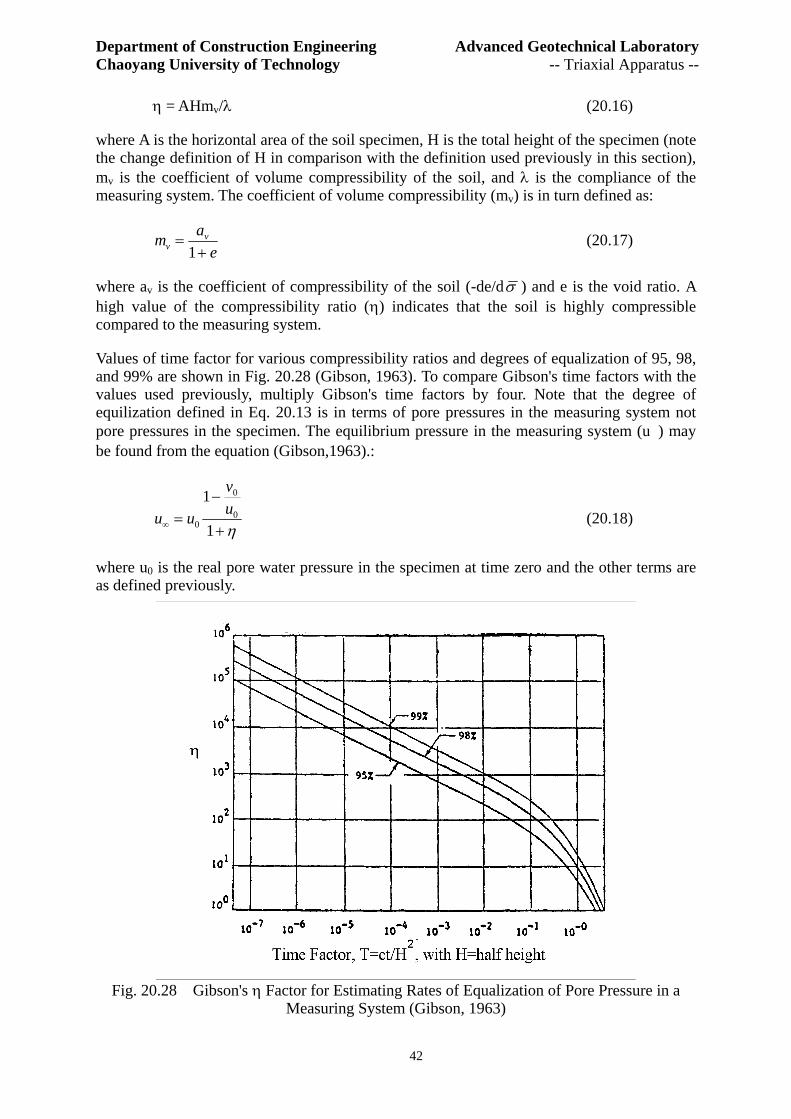
Department of Construction Engineering Advanced Geotechnical Laboratory Chaoyang University of Technology -- Triaxial Apparatus --
42
η = AHmv/λ (20.16)
where A is the horizontal area of the soil specimen, H is the total height of the specimen (note the change definition of H in comparison with the definition used previously in this section), mv is the coefficient of volume compressibility of the soil, and λ is the compliance of the measuring system. The coefficient of volume compressibility (mv) is in turn defined as:
e
am vv +
=1
(20.17)
where av is the coefficient of compressibility of the soil (-de/dσ ) and e is the void ratio. A high value of the compressibility ratio (η) indicates that the soil is highly compressible compared to the measuring system.
Values of time factor for various compressibility ratios and degrees of equalization of 95, 98, and 99% are shown in Fig. 20.28 (Gibson, 1963). To compare Gibson's time factors with the values used previously, multiply Gibson's time factors by four. Note that the degree of equilization defined in Eq. 20.13 is in terms of pore pressures in the measuring system not pore pressures in the specimen. The equilibrium pressure in the measuring system (u∞) may be found from the equation (Gibson,1963).:
η+
−=∞ 1
10
0
0uv
uu (20.18)
where u0 is the real pore water pressure in the specimen at time zero and the other terms are as defined previously.
Fig. 20.28 Gibson's η Factor for Estimating Rates of Equalization of Pore Pressure in a
Measuring System (Gibson, 1963)

Department of Construction Engineering Advanced Geotechnical Laboratory Chaoyang University of Technology -- Triaxial Apparatus --
43
The problem now is to determine the compliance of typical pore pressure measuring systems. The compliance of an electronic pore pressure transducer is of the order of 4x10⁻⁷ in3/psi (Whitman, Richardson, and Healy, 1961). The coefficient of compressibility of water is of the order of 3.4x10⁻⁶ in3/in3/psi. Poulos (1964) measured the compliance of typical values used in pore pressure measuring systems and found the following average values:
needle valves 10-40 x 10-8 in3/psi Klinger plug valves 20-60 x 10-8 in3/psi NGI Piston Valve 60 x 10-8 in3/psi Circle Seal Plug Valve 20-200 x 10-8 in3/psi
These compliances will vary from valve to valve and should be considered only approximate. Hirschfeld found the compliance of 1/4-inch O.D. by 1/16- inch I.D. Saran tubing to be about 20x10-8 in3/in/psi. Pennman (1958) found a compliance of 2.8 mm bore by 1 mm wall type 6/6 nylon tube to be 50x10-8 in3/in/psi. Pennman (1956) also measured the compliance of 3 mm bore by 1 mm wall polyethylene tubing and found it to be about 200x1010-8 in3/in/psi. The compliance of tubing may be estimated from the equation:
Etdi
4
3πλ = (20.19)
where Di is the inside diameter of the tubing, t is the wall thickness, and E is the elastic modulus of the tubing material.
Based on these data the engineer can easily estimate the compliance of the proposed measuring system and ensure that it is sufficiently low (using Gibson's theory) so that it need not be considered further.
One additional factor that may cause problems is temperature change. The problem is most important for relatively impervious and incompressible samples and for the case that the transducer is separated from the triaxial cell by a length of relatively incompressible tubing (Olson, 1963).
MEMBRANE PENETRATION EFFECTS
In reducing data from triaxial tests/ the assumption is generally made that the membrane exists at the outside lateral boundary of the specimen. However, for tests with relatively coarse-grained soils, the membrane penetrates into the interstices between the outer layer of particles. The result is an error in volume change calculations. The error involves calculation of the area of a sample. It also impacts on R and R tests where the assumption of constant volume is invalidated by membrane penetration that occurs during shear.