1

APFO’s Public ArcGIS Server: Set-up and Use

The instructions will discuss the folders available on the public NAIP server in the following order:

I. Adding Data from APFO’s Public ArcGIS Server into ArcMap 10.x

(pg. 2) II. NAIP Imagery Available on the Server (pg. 4) III. Additional Data in the NAIP Folder (pg. 7)

1. Imagery Dates (pg. 7) 2. NAIP Acquisition Status Map (pg. 10) 3. NAIP Inspection Status Map (pg. 10)

IV. Imagery for the Hawaiian Islands (pg. 11) V. The Base Map (pg. 13) VI. The Reference Folder (pg. 15) VII. The Maps Folder (pg. 21)

The Utilities folder is empty.

The first three folders display imagery, and the last two display vector data.

The “short instructions” for accessing this service states that the URL is https://gis.apfo.usda.gov/arcgis/rest/services

This is a change from the previous URL. The important difference is the addition of an “s” after http. Also, /rest/ is inserted between arcgis and services. (The URL probably also works without this word.)

2

I. Adding Data from APFO’s Public ArcGIS Server into ArcMap 10.x

APFO provides the most current year of NAIP imagery in a web service for public GIS users. The service also offers imagery for Hawaii and some other areas. There are a number of other layers which are useful in researching NAIP or historical film photography from the NAPP or NHAP programs archived at APFO. There is also a collection of basic map information, such as county or PLSS boundaries, cities, highways, and water bodies.

The detailed instructions for adding the service into ArcGIS 10.x:

1) Open ArcMap and Click the Add Data button.

2) Select GIS Servers and then Add ArcGIS Server. Click Add.

3) Click the Use GIS Services radio button, and then click Next.

4) In the Server URL: text box enter https://gis.apfo.usda.gov/arcgis/rest/services .

5) Click Finish.

3

A new server, arcgis on gis.apfo.usda.gov, has been added to the GIS Servers list. Double Click the new ArcGIS Server connection to access the server.

The server will probably be used most frequently to access the most current NAIP imagery for a state or states. NAIP was acquired for the 48 contiguous states in the country. There is also imagery available for Hawaii in a separate folder.

The server has several additional map layers, displaying information such as state and county boundaries, water bodies, cities, highways, UTM zone lines, and NAIP acquisition and inspection status maps. These layers may change from time to time, and cannot be edited.

4

II. NAIP Imagery Available on the Server

After connecting to the server, double click the NAIP folder to see the state based imagery services.

A list of state based image services in natural color format for the most current flying year will open. Select from the list, and view the selected state in a GIS document.

5

The server displays only the most current year of imagery; for Pennsylvania, that was 2015.

At present, the NAIP imagery in the public web service can displayed as either Natural Color (Red, Green and Blue bands) or Color Infrared. The user has the option of selecting the band combination to display. Instructions for setting the bands:

1) Right click the name of the imagery to display. Select [Layer] Properties at the bottom of the drop down menu.

2) After the Layer Properties window opens, select the Symbology tab

3) Select the bands by clicking on the small arrows to the right of the Channel and Band

columns. For Natural Color, Red should be set as Band_1, Green as Band_2, and Blue and Band_3.

4) For Color Infrared, Red should be set as Band 4, Green as Band_1, and Blue as Band_2.

Band_3 will not be used.

6

Band settings for a Color Infrared display. The Stretch is set to None

Band settings for a Natural Color display. The stretch has been turned off.

7

III. Additional Data in the NAIP Folder

1. Imagery Dates

In addition to the most current year of imagery, the web service also offers a vector layer, called NAIP Image Dates, giving information about the project’s acquisitions in every part of the state. These “seamlines” delineate the flight lines or “exposures” (this varies with the sensor) which captured the area of the image lying within its boundaries.

Selecting the NAIP Image Dates layer

The seamline files are listed by year, for 2015 and 2014. The year and state will need to be selected by checking the box next to the name. The colors for the seamlines and for the labels cannot be changed, and they may be difficult to see. The labels can be selected by right clicking next to the state name and checking Show Labels. The labels will display at a scale of 1:250,000 or larger.

8

Lancaster Co, Pennsylvania, displaying seamlines and dates.

The attributes for each polygon can be accessed. They will tell the date of flight (IDATE), the starting and ending times, with the date (SDATE and EDATE), and the band content (BCON – this will be MB4, which indicates four bands – red, blue, green and color infrared.) The web display can be changed from the natural color version to color infrared. Four band DOQQs can be purchased from APFO if users want to process the imagery.

The attributes also include the camera type, manufacturer, and model (CAM_TYPE, CAM_MAN, and CAM_MOD), the camera hardware firmware (HARD_FIRM), the sensor number (SENSNUM), and the aircraft type and tail number (AC_TYPE, ACTAILNUM). The vendor’s name is not given.

Beginning in 2014, the seamline files also displayed the electromagnetic spectrum ranges for the four bands collected.

9

10

2. The NAIP Acquisition Status Layer This map displays the acquisition status for the given year, by county. The display is either dark maroon (Acquired) or gold (Received.)

3. The NAIP Inspection Status Layer This map shows the status of the NAIP imagery inspection process. When an inspector completes a phase of the inspection, and enters this information into APFO’s Oracle database, the symbology on the map changes.

11

IV. Imagery for the Hawaiian Islands

1) Double Click the Hawaii folder to see the Hawaiian imagery service.

2) There is only one option to select for Hawaii, from 2011.

3) The imagery for Hawaii came from different sources. Some of it may be satellite

imagery, and some of it may be aerial imagery from agencies such as NRCS. The imagery source is not listed.

12

13

V. The Base Map

The folder entitled Base Maps contains one map, also called Base Map. This is a color shaded relief map which displays at scales smaller than 1:1,500,000. At scales larger than 1:1,500,000, NAIP Imagery is displayed.

Shaded Relief Map (scale smaller than 1:1,500,000)

14

NAIP imagery (scale larger than 1:1,500,000)

15

VI. The Reference Folder

This folder contains a USA Base Map which is different from the Base Map described in section IV (above).

It contains a good deal of useful vector data which can be turned on or off through the Table of Contents. Some data only displays at certain Zoom levels. The Cities layer displays cities and towns when zoomed in to 1:200,000 and closer.

16

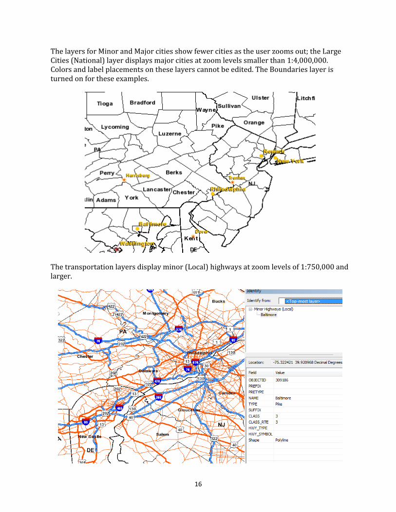
The layers for Minor and Major cities show fewer cities as the user zooms out; the Large Cities (National) layer displays major cities at zoom levels smaller than 1:4,000,000. Colors and label placements on these layers cannot be edited. The Boundaries layer is turned on for these examples.

The transportation layers display minor (Local) highways at zoom levels of 1:750,000 and larger.

17

Fewer roads are displayed when zoomed out to the Major Highways (Regional) layer. From 1:1,500,001 to 1:20,000,000 the user sees the Freeway System (State). Zooming out further shows the Freeway System (National).

The Topographic Map Indices layers display USGS indices ranging from the UTM Zones to the Quarter Quads. This example, displaying from 1:150,001 to 1:500,000, shows the quadrangles, with the familiar Quad name in the attribute table. These indices are useful in locating individual DOQQs.

18

Under the Land Management/Public Land Survey System (PLSS) layer, the Township and Range boundaries appear when zoomed in to 1:250,000 or closer.

State plane zone boundaries (in yellow) appear between 1:3,000,001 and 1:8,000,000. These ranges, labels and colors cannot be edited.

19

An example from the Land Management /Federal Lands layers, shown below, displays National Forests (light green), National Parks (medium green), Department of Defense (orange), BLM lands (sand), and the Navajo and Hopi lands (light brown)lands.

20

The USA Boundaries layer displays state and county boundaries, depending upon the zoom level. The Water layer, shown below at the Regional zoom levels, displays major rivers, creeks, and lakes (only as polyline boundaries.)

The Pacific Basin layer does not display.

21

VII. The Map Folder

The GIS Viewer displays additional information, which was available originally in shapefile or feature class format. Much of it was used by the APFO Customer Service Section in researching sales orders. The GIS Viewer is on the APFO website, and the Historical Availability layer is on ArcGIS Online.

The web map for Historical Availability on ArcGIS Online can be accessed at: http://www.arcgis.com/home/webmap/viewer.html?webmap=03e5dfa695b24a48bf5f5bf14c633416

This map displays the number of years of film and digital imagery for each county.

Entries stating “FSA” were actually ASCS film in the 1950s - 1980s.

22

APFO has photo center files for film acquired through the National High Altitude Program (NHAP), National Aerial Photography Program (NAPP) and National Agriculture Imagery Program (NAIP). Pictured below are NAPP1 points.

The center points for NAPP 2 and 3 are in the same position, and the point symbols will be on top of each other. A zoomed in view displays the roll and exposure for each of the available exposures at that site, and the labels are color coded to match the symbol for each NAPP photo program. The points will not appear at scales smaller than 1:250,000. The Maps Folder also contains some Geographic Layers – Cities, Highways, Water, and Land Management. The Land Management layers include PLSS, USGS indices, and Federal Lands. The example below show National Forest, National Park, and Bureau of Indian Affairs lands. The folder does not have as many options as does the Reference folder.

23

The SAAP Status map displays acquisition and inspection status information for small area projects flown for other agencies. This imagery is not available to the general public, and the map is for agency use.