WjPs(1Zc.POLICY RESEARCH WORKING PAPER 188.

A4 e, .,Ufss e., he

Economic Transition MdJrsl sgethAp M ;rfhe -n;

and the Distributions a

of Income and Wealth mark'tSy4,of'the '-

.pd ??3j pubi goo ;

- rPer. ,th~t prevent theFrancisco H. G. Ferreira

--tne tivate sec and

eWnsirq tha t.subl - .e

nets, ae in place.

The World BankOffice of the Chief Economnist for East Asia and PacificAugust 1997

Pub

lic D

iscl

osur

e A

utho

rized

Pub

lic D

iscl

osur

e A

utho

rized

Pub

lic D

iscl

osur

e A

utho

rized

Pub

lic D

iscl

osur

e A

utho

rized

POLICY RESEARCH WORKING PAPER 1808

Summary findings

Using a model of wealth distribution dynamics and Creating new markets in services that are also suppliedoccupational choice, Ferreira investigates the by the public sector may also contribute to an increase indistributional consequences of policies and developments inequality. So can labor market reforms that lead to aassociated with the transition from central planning to a decompression of the earnings structure and to greatermarket system. flexibility in employment.

The model suggests that even an efficient privatization The results underline the importance of retainingdesigned to be egalitarian may lead to increases in government provision of basic public goods and services,inequality (and possibly poverty), both during the removing barriers that prevent the participation of thetransition and in the new steady state. poor in the new private sector, and ensuring that suitable

safety nets are in place.

This paper - a product of the Office of the Chief Economist for East Asia and Pacific - is part of a larger effort in thedepartment to understand the effects of economic transition on the poor. Copies of the paper are available free from theWorld Bank, 1818 H Street NW, Washington, DC 20433. Please contact Michael Geller, room N7-101, telephone 202-473-1393, fax 202-522-0056, Internet address fferreira@worldbank.org. August 1997. (44 pages)

The POliPY Research Workodng Paper Serbs disseminates the findings of work in progress to encourage the exchange of ideas aboutdevelopmnent issues. An objective of the series is to get the findings out quickly, even if the presentations are less than fully polished. Thepapers carry the names of the authors and should be cited accordingly. The findings, initerpretations, and conclusions expressed in thispaper are entirely those of the authors. They do not necessarily represent the view of the World Banke, its Executive Directors, or thecountries they represent.

Produced by the Policy Research Dissemination Center

ECONOMIC TRANSITION AND THE DISTRIBUTIONS OFINCOME AND WEALTH

Francisco H.G. Ferreira1

The World Bank

Keywords: Transition economies; Privatization; Inequality; Wealth distribution.

JEL Classification: D3 1, D63, H42, P21.

Correspondence Address: The World Bank; 1818 H Street, NW; Washington, DC20433; USA. E-mail: fferreiragworldbank.org

I am grateful to Simon Commander, Tito Cordella, Aart Kraay and participants at a conference at theEBRD in London for helpful comments and discussions.

2

1. Introduction.

In 1987, two years before the fall of the Berlin Wall, some 2.2 million people lived on

less than U$1-a-day (in 1985 prices, using PPP exchange rates for each country) in

Eastern Europe and the former Soviet Union. In 1993 - a mere six years later - with

economic reform in full swing throughout the region, that number had risen almost

sevenfold to 14.5 million.2 Over this period, and with respect to that poverty line, the

region had recorded by far the largest increase in poverty (as measured by the headcount)

of any region of the world, even if it still had the lowest average headcount in the

developing world.

This unprecedented increase in serious poverty, in a region where it had been almost

eradicated, was due fundamentally to two effects of economic transition on its income

distributions: a fall in average household incomes, sustained during the period of output

collapse; and an increase in income and expenditure inequality, which is almost as

pervasive a feature of the transition process as the first. But even if the declines in output

- which took place in every country in the region, albeit to different extents (see EBRD,

1995) - may have been the main culprits for the increases in poverty, they may prove less

persistent. The output declines have now been completely or partially reversed in a

number of transition economies, and the others look set to follow suit. Though they were

severe and their impact on living standards was dramatic, they were essentially transitory

phenomena; part of the transitional dynamics in moving from one steady-state to another,

rather than characteristics of the new steady-state.

The same can not so confidently be said of the substantial increases in inequality.

Transition economies, whether in Eastern Europe and the FSU or elsewhere, consistently

reported some of the largest increases in Gini coefficients between the early 1980s and

the early 1990s among the countries in the Deininger and Squire international inequality

2 According to the World Bank (1996).

3

data-set. Poland's Gini rose by 7.3 percentage points (pp) between 1982 and 1993;

Hungary's was up by 6.9pp over the same period; Russia's rose by 5.9pp in 1980-1993.

The Chinese Gini rose by 7.3pp between 1981 and 1994. And there has been no

indication that this trend is about to be reversed.

Despite data limitations, much has already been written on this distributional effect, and a

considerable body of empirical evidence is emerging on the dynamics of income

distributions in transition economies, through works such as those by Atkinson and

Micklewright (1992), Commander and Coricelli (1995) and Milanovic (1997). The

picture of widespread and pronounced increases in income, expenditure or earnings

inequality which arises from this evidence is remarkable, particularly when contrasted

with the general stability of income distributions in most other countries for which data is

available. Based on their recent international compilation of inequality measures from

household survey data sets, Deininger and Squire (1996) found that inequality does not

tend to vary a great deal over time within given countries - though it varies rather

dramatically across countries.3 The recent experience of economies in transition, with 5-

7.5 percentage point rises in Gini coefficients not uncommon, is clearly exceptional.

What lies behind it? What is it about the process of transition from central planning to a

market system which appears to involve an inherent increase in inequality? Is this

increase likely to be transitory, or could it be permanent? What policy reforms in the

menus suggested to governments are likely to cause these increases in income dispersion?

How do they do so? This paper seeks to suggest some answers to these questions, by

investigating the effects of policies and processes associated with economic transition on

the equilibrium distribution generated by a model of wealth distribution dynamics with

imperfect capital markets. It relies on a variant of the model discussed in Ferreira (1995),

"The measures are relatively stable through time, but they differ substantially across regions, a result thatemerges for individual countries as well [... ]The average standard deviation within countries (in asample of countries for which at least four observations are available) is 2.79, compared with astandard deviation for the country-specific means of 9.15." (Deininger and Squire, 1996, p.583.)

4

which draws on insights developed in a growing literature, including works by Aghion

and Bolton (1997), Banerjee and Newman (1991 and 1993), Benabou (1996), Galor and

Zeira (1993) and Piketty (1997). It is hoped that some of the propositions arising from

this conceptual exercise might be of use in suggesting fruitful avenues for future

empirical research into the causes of growing inequality in transition economies.

Income distributions are determined by the underlying distributions of assets, and by the

rates of returns on those assets. One can think of a household's income as the inner

product of the vector of assets it owns (land; shares; bonds; the skills of its members) and

the vector of prevailing returns on those assets (rent, actual or imputed; dividends;

interest; the wage rates accruing to the different skills). In an uncertain world, some or all

of these returns may be stochastic, so that there is a probability distribution associated

with each of them, and consequently a random component to the determination of

incomes. In principle, therefore, changes in the distribution of income can be due to

changes in the distribution of ownership of one or more assets, or to changes in the

returns associated with them, or yet to changes in the probability distributions associated

with shocks inherent to the income generating process. In the sweeping changes of

transition in Eastern Europe and the FSU, it is likely that all three types of changes have

played (and continue to play) a role.

This paper focuses on three groups of possible sources of changes in the distribution of

income: the privatization of public assets; the development of new markets in privately-

provided substitutes to public services (e.g. telephones, schools, health-care); and changes

in the returns associated with different skills (i.e. on the earnings-education profile). The

first of these leads to a change in the underlying distribution of asset ownership, but we

will show that it is also likely to impact on wages in the public sector, thus affecting

returns. Privatization can be shown to affect the distribution of income by changing

ownership, wages and occupational choices. The creation of new markets in privately-

provided substitutes to public services will be shown to affect the returns on assets, and to

do so differently for different wealth levels. The new markets are likely to enable richer

5

agents to top-up public provision, thus increasing the expected returns from their assets as

compared to poorer agents. Finally, increases in the returns to education and skills, as

well as the greater volatility associated with employment and earnings in a flexible labour

market, are likely to lead to increases in earnings inequality.

Although we consider both short-term and long-term impacts of these changes, the

analysis ignores a number of transitory effects which may well have contributed

substantially to the increases in inequality and poverty early on in the process of

transition. Notable amongst these were increases in the rate of inflation, which were

known to have hurt those on fixed incomes who did not have the political clout to

readjust them often (e.g. pensioners and some public employees), much more than those

able to readjust their prices more frequently.4

The paper is structured as follows. Section 2 presents the basic model: it describes the

supply and demand side characteristics of agents, the government sector and the financial

markets; section 2.1 outlines the static equilibrium of the model, by describing the actions

and incomes of all agents as functions of their initial wealth and of a random variable;

section 2.2 relies on those income processes to characterize the transitional dynamics of

this stochastic system and the (steady-state) limiting distribution to which it converges.

Section 3 considers the effects of privatizing part (or all) of the state-owned productive

assets: it first investigates the short-term effects, through impacts on public-sector wages

on the one hand, and higher income from (privatized) capital on the other; then it

considers the permanent changes after the one-off windfalls from privatization have been

absorbed into the dynamics of the system. Section 4 introduces markets for privately-

provided substitutes to public services. This reform is found to add to economic

efficiency, as was to be expected from eliminating a missing market problem, but also to

add to inequality. Section 5 provides an informal discussion of the factors likely to affect

4 See Ferreira and Litchfield (1997) for an empirical analysis of the effects of high inflation on theBrazilian income distribution in the 1980s.

6

the returns to different skills, and hence the returns to education and the distribution of

earnings. Section 6 summarizes the findings of the paper and concludes.

2. The ModeL

Let there be a continuum of agents with wealth distributed in [0, ul, with total mass 1. At

any time t, their distribution is given by Gt (w), which gives the measure of the population

with wealth less than w. G, (u) = 1 for all t. These infinitesimal agents can be thought of

as household-firms, identical to one another in every respect other than initial wealth.

Their size is normalized to one. Each agent is risk-neutral, lives for one period and has

one offspring. The sequential pattern of their lives is as illustrated in Figure 1 below:

Figure 1:

I I I I I lbirth receive invest receive pay tax consume

(receive any transfers return reproducebequest) bequeath, die

There is a single consumption good in the model, which can be stored costlessly across

periods. Agents seek to maximize:

U(c, ,b, ) = hc,a b,-a (O<a<l) (1)

where ct denotes the agent's total consumption in period t (her life), and bt denotes the

bequest she leaves her only child. The formulation in (1) implies the "warm-glow"

bequest motive (see Andreoni, 1989). This is clearly a short-cut approach to full

intertemporal optimization, but it is one which has been extensively used in the literature,

given the simple dynamic structure it implies for the wealth process. It is not entirely

innocuous, and replacement with full intertemporal optimization - where the Keynes-

Ramsey rule holds - would change the model and generate additional insights. A

discussion of the implications for this model is contained in Ferreira (1996).

7

On the supply side, agents may choose between two alternative occupations: they may be

public sector employees, working for a deterministic wage o, or they may set up on their

own as private sector entrepreneurs, in which case they face a stochastic production

function given by:'

Yt = 0 if k < k' (2)

yt= 0t rkt ifk2k'

where k is private capital and 0 is a random variable distributed as follows:

0 = 1 with probability q

0 = 0 with probability 1-q and q:= v-'(g/k)

g denotes the quantity of public capital used in the production process. The important

properties of v are that it is defined on domain [0, 1], and that v' > 0. But it will be

convenient to assume the following specific form for v: g/k = qy , where O<a<1. This

implies that q = (g/k)a, and that

E(y, Ik > k') = rklaga. (2')

Once one of these two occupations is chosen, agents are assumed to allocate their full

effort to it, and to it alone, so that effort supply is completely inelastic, and convex

combinations of the two activities are ruled out.

Before turning to the capital markets and the role of government, it may be useful to

spend a moment discussing the stochastic private sector production function just

described. In this private sector, there is a minimum scale of production, given by an

amount of private capital k' > 0. This non-convexity in the production set captures the

minimum costs of going into business, which can range from the cost of a plot of land, or

an industrial plant in which to locate machines, to the cost of a licence to operate a kiosk

or of a stall on which to display vegetables in a street market.5 Once that minimum scale

Similar minimum scale or more restrictive fLxed scale assumptions are common in the literature. See e.g.Aghion and Bolton (1997), Galor and Zeira (1993) and Banerjee and Newman (1993).

8

has been reached, agents face stochastic returns to private capital, where the probability

of success rises with the ratio of public capital to private capital. This is meant to capture

both the uncertainties and risks associated with private sector activity, as well as the

complementarity between certain types of public and private capital, which has been

frequently noted in the growth literature (see e.g. Barro, 1990 and Stern, 1991.)

The nature of 'public capital' g requires elaboration. Just as there is an enormous array of

goods and services in the world, all of which are subsumed under the aggregate

consumption composite c, there also exists a large and complex range of non-labour

inputs into production, which are routinely lumped together in macro models as 'capital'.

It has long been recognized both that there are externalities associated with at least some6types of capital , and that different types of capital can be complements (computers and

education of those using them) or substitutes (delivery vans and delivery motorcycles).

Combining these two ideas, let us divide the various forms of capital into two broad

groups: forms of capital with limited or no externality generation are aggregated as k and

called private capital. It is hard to think of justifications for public provision of this sort of

capital in a fully functioning market system in which the usual efficiency advantages of

private producers over the public sector are present. Other forms of capital are

characterized by high positive externalities associated with their use or production (the

best examples may be forms of human capital, such as education and health, or physical

infrastructure capital with a strong network dimension, such as streets, rural roads,

telecommunications or power). These are aggregated as g, and named 'public capital'.

What defines g is the presence of positive externalities in production or use. These inputs

are not public goods: they are in fact assumed to be excludable in use. Two things

follow: first, there may be justification for public involvement in producing (or financing)

6 Famous for having enabled modelers to combine constant returns to an accumulatable factor andcompetition, helping to endogenize growth in per capita output; see Arrow (1962) and Romer (1986).

Some may be club goods, in that they are excludable but non-rivalrous.

9

some of this capital directly, because government failures (e.g. red-tape or shirking) may

be outweighed by market failures (externalities or high transaction costs). Second, there

will nevertheless be scope for private production of some of this capital too. Our

aggregate public capital g is likely to be produced both by public and by private sector

agents, as is indeed the case with education services, health care or telecommunication

services.8

Whoever produces it, 'public capital' contributes to private production in this stochastic

setting by raising the probability of its success: the better the health care available to your

farm labourers, the less likely they are to succumb to a preventable epidemic, leaving

crops untended; the more reliable the power supply and the telephone system, the less

likely it is that consumers will be disappointed by your own reliability; the better the rural

roads (g), the likelier it is that your lorry (k) will deliver produce to market.9 In this sense,

private and public capital are therefore complements in the stochastic production function

of the private sector. Given the specific form assumed for the v function, the expected

output from private-sector production turns out to be homogeneous of degree one in k and

g-

Let us now turn to the role of the governnent. This role is perhaps the most important

thing that changes in the process of transition from central planning and government

ownership of the means of production to a market economy. It may therefore be helpful

to describe three plausible governments, one for each stage of the transition: before,

during and after.

Government B is the stylized picture of the owner of all means of production. It combines

labour and capital according to the Leontieff production function:

8 We explore the consequences of allowing for this 'topping-up' of public capital from private sources in alater section.

The probability is a function of g/k: if your lorry is a 30-ton articulated container truck, it needs betterroads to make it to the market.

10

Xi = min(crS,,)LLs,) (3)

where X denotes the output of the state sector, S denotes the stock of capital used by the

government, and L. denotes the size of public sector employment. The practice of labour

hoarding, which is widely documented to have been common in centrally planned

aeconomies, is incorporated by assuming that L,, > - S,, so that in effect X, = aS,. For

simplicity, assume that S does not depreciate. Government B has discretion on how to

distribute output X,. One plausible such distribution rule, compatible with the ideal of

equality of outcomes, is to set wages equal to the average product of labour:

X, aS,

Lst Lst

Equation (4) is a distribution rule, a wage setting equation and, since this government

administers all production and has no need to tax, it is also Government B's budget

constraint. One can think of the wage X as incorporating any in-kind benefits, such as

child or health care, made available to public sector workers in this economy. In this

benchmark case, no g is produced, so that there is no private sector. Public employment

exhausts the total labour force: L. = L. There is perfect income equality with a Dirac

distribution at o.

Government A is the stylized benevolent government in a mature market economy. In

such an economy, there are govemment failures (particularly pervasive in producing

consumption goods or private capital, so that these are produced by private agents) and

market failures (which outweigh government failures in the production of some goods,

which are here all assumed to be in the public-capital category). This government seeks

9

to maximize a linear social welfare function given by: W = fy(w,O)dG(w) subject to:0

gg JdG(w) = T Jy(w,O)dG(w) (5)0 0

11

The budget constraint in equation (5) summarizes four key (assumed) restrictions in the

policy choices available to benevolent government A. First, the government can not levy

lump-sum taxes. Hence, in this set-up with inelastic labour supply, income taxes are

quasi-lump-sum and are preferable to taxing either consumption or bequests only, or both

at different rates.'0 Second, the government can only tax incomes proportionately, at a

constant rate x, without exceptions. Third, the government can not make cash transfers.

Fourth, the government can not target the in-kind transfers of public capital which it

makes (perhaps due to the administrative costs involved). These are hence distributed

uniformly to all agents, who receive an amount g5." The transformation from tax

revenues into in-kind transfers of public capital is deliberately not modeled explicitly: it

may be more efficient for the government to finance production by private agents, or it

may produce them directly, through some implicit production function using the tax

revenues.

The third kind of government, D, is a hybrid of the other two. It is a government in

transition, and hence combines functions from both B and A. It retains a sector producing

the consumption good c, with technology (3), and a modem sector producing public

capital goods g, which it distributes uniformly to the population, like A. Its budget

constraint is given by:

o°L, + gg |dG(w) =T w,O)dG(w) + X (6)0 0

I continue to assume that the public-sector wage is set in accordance to (4), so that there

is no cross-subsidy between the two sectors of this transitional government. I also assume

that gg has been historically determined at some exogenous level (perhaps by some vote

10 Given preferences in equation (1), taxing c and b at identical rates is equivalent to taxing incomes. For adiscussion of the public economics of this model, see Ferreira (1996).

11Since JdG(w) = 1, the reader can for the moment think of g8 either as an amount of an (excludable)0

private good uniformly distributed to all agents, or alternatively as the amount of a (non-excludableand non-rivalrous) public good, which any agent can use in his or her production function. Thissecond interpretation must only be abandoned in Section 4.

12

early in the process of transition) and r adjusts to satisfy (6). 12 Since we are concerned

with the process of economic transition, in the analysis below govermment will always be

this government D.

Finally, I assume that credit markets work imperfectly. The important requirement is that

there exist credit ceilings linked to agents' initial wealth levels. This can be obtained

through a set-up like that in Banerjee and Newman (1993), based on imperfect

enforcement of repayments, but the insights are the same if the credit markets are simply

assumed away altogether. For simplicity, this is the route taken below, where we assume

agents can not borrow (or lend) at all. Savings are simply stored and, like capital or

bequests, do not depreciate.

2.1. The Static Equilibrium.

The objective of this sub-section is to determine how the occupational choice between

public and private sectors is made by each agent, and to describe her end-of-period (pre-

tax) income as a function of her initial wealth level and of her drawing of the random

variable theta. This will allow us to characterize the transition function of wealth, which

will provide the basis for investigating the long-run dynamic properties of the system. To

focus on an economy in transition, I assume that the government is Government D. The

existence of a minimum scale requirement for private sector production (k 2 k') implies

that there will be three classes in this simple version of the model, subject to the

following restriction:

Assumption 1: Given the private sector rate of return r, the historic level of gg is

sufficiently high in relation to the productivity of labour in the public sector that, at the

12 The more satisfactory approaches of modeling the choice of T explicitly in a voting framework, oralternatively assuming a benevolent dictator which maximizes social welfare by choice of an optimalr*, introduce too much complexity for the purposes of this paper. However, see Ch. 4 in Ferreira(1996) for a cut at the latter approach. The alternative route of fixing Xr at some exogenous level hereis just as unsatisfactory, and would add unnecessary complications.

13

minimum scale of private production, expected end-of-period income is higher in the

private sector than in the public sector. In other words, if we denote (pre-tax) income in

the private sector yp and income in the public sector yG:

E[yIw= k' ]> E[yGIw= k']

rkt-ag' >co + k = aS +k, (7)9 ~Ls

In addition to this assumption, we will also need one more result to fully characterize the

three social classes. Let wu denote the upper bound of the wealth interval supporting the

ergodic distribution G*, the limiting wealth distribution towards which the system

converges. w% is defined below in equation (10).

Lemma 1: The upper bound of the support of the limiting wealth distribution, w., is

sufficiently high that the marginal product of capital there is below 1:

E[MPk(w. )] < I => r(l -a)w.- g.. < 1

Proof: See Appendix.

Figure 2 below illustrates the meaning of Assumption 1 and Lemma 1. Assumption 1

requires that the expected income from private sector production at k' be greater than the

(riskless) income which can be derived from working as a public sector employee. The

latter is equal to the wage a) plus the initial wealth (the return on which is 1, since there

are no capital markets and no depreciation). Lemma 1 establishes that the expected

marginal product of capital in private production (the convex curve in the bottom panel of

Figure 2) is less than 1 at the upper bound of the wealth interval supporting the ergodic

distribution (we). If we implicitly define w, as E[MPk (wj)] = 1, then it requires that wC <

wU.

14

Figure 2

E(y) rk g

k. k

E[MPk]

IE[MPk] = r(I-a)k"aga

Wc k

We can now describe end-of-period incomes for all agents, as follows:

Proposition 1: In the economy described so far, there are three classes of agents, defined

by their occupation and sector of employment: the poorest agents, with wealth w < k',

work in the public sector for a deterministic wage aD. All agents with wealth greater than

or equal to k' choose to become entrepreneurs in the risky private sector. But there are

two classes of entrepreneurs: those with wealth between k' and wC invest all their wealth

in the production function (2); while those with wealth greater than wC save some of it.

The end-of-period (pre-tax) income function is therefore given by:

15

y,(w,,0,)= o, +w, for w, e[O,k')

0 ,rw, for w, e[k',wC) (8)

0 rw, + (w, - W) for w, E[WC ,u]

Proof: 1) Agents with wealth w < k' work in the public sector because:

E[yG I w < k'] = o + w > E[yp I w < k'] = 0. The first equality arises from earning wage

co from one's labour in the public sector and saving one's initial wealth. The second

equality arises from the minimum scale requirement in production function (2).

2) Agents with wealth k' < w < w, invest their full wealth in the private sector

because:

* Assumption 1 ensures that it is worth investing at least k' in the private sector, and

* Lemma 1 and the fact that E[ MPk] < 0, Vk ensure that it is also preferable to investak

any wealth up to wc, rather than to save it. Once they invest their full wealth w (> k') in

production function (2), their return is Ot rk,.

3) Agents with wealth w > w; find it profitable to invest wC in the private sector

because rw-g'> co + w., which follows from Assumption 1, Lemma 1 and the

monotonicity of MPk. Given Lemma 1, however, it is clearly optimal for them to save

(w- wc) rather than invest it.

2.2. Transitional Dynamics and the Steady-State Distribution.

The utility function in (1), implies that bequests are a fixed proportion of the after-tax

end-of-period income for each and every agent: b, = (1 - a XI - X)y, , where yt is defined

in equation (8) above. Since bt = wt+i for each lineage, the intergenerational law of

motion of wealth in this model can be written simply as:

w,+, = (1- a)(l-,)y,(w, 0,) (9)

16

where y, (w, ,O, ) is defined in equation (8).

Otis not i.i.d., because it is not identically distributed over time, since the probability q (

v I(g/k)) may change from period to period. Nevertheless, since g, is predetermined and kt

depends only on the current (period t) value of wealth, Ot is independently distributed. a

and T are time invariant exogenous parameters. It follows that there are no indirect links

between previous values of w and wt+j or, in other words, that for any set A of values of

wealth, Pr (wt+ E A I wt, w wtl,..., w ,...) = Pr (wt+1 E A I wi). The transition process of

wealth is therefore a unidimensional Markov process, which allows us to be fairly

specific about the long-run properties of this dynamic stochastic system, as shown by the

following proposition:

Proposition 2: The stochastic process defined by equation (9) is a Markov process, with

the property that the cross-section distribution Gt(w) converges to a unique invariant

limiting distribution G*, from any initial distribution Go(w).

Proof See the proof of proposition 3 in (the appendix to) Ferreira (1995).

It is intuitive to see that the upper bound of the ergodic wealth set (the support of G*)

must be the highest level of wealth which generates a bequest no smaller than itself.

Substituting y, (w,,O,) = O,rw, + (w, - w,) - for w, e [w, u] and 0 = 1 - from equation

(8) into (9), and requiring that wt+I = wt solves for wu:

WI, = (I a)(I-)r-lW (10)

where, of course, Lemma 1 implies that (I1 X 1) > 1.

Figure 3 below illustrates the wealth transition function given by equation (9). The

bequests left by agents in each class are simply a fraction (1 -a)(1 -'r) of their end-of-

17

period incomes, as given by (8). While there is a single bequest function in [0, k'), where

incomes are deterministic, there are two in [k', wj, one for 0 =0 and one for 0 =1. The

slope of the bequest function is therefore (1-a)(1-') in [0, k') and for both functions in

[wc,wj]. For the middle-class in [k', wj] the function for 0 =0 is a constant at zero, while

the upper line (for 0 =1) has a slope of (l-a)(l-t)r. To avoid poverty traps, I assume that

(I -a)(1-T)(co + k') > k'.'3 This and assumption 1 then imply that (l-)(1-X)r>1.

Figure 3 wt+, 450

`01

* ~~~~00

0 k' wC wU w

The implication of Proposition 2 and of the specific transition function given by equation

(9) is that the long-run equilibrium of this stochastic process is characterized by an

invariant non-degenerate wealth distribution, with three 'social classes' defined by the

choice of occupation and/or investments undertaken by agents. The poorest agents choose

to work in the less productive public sector, because the missing credit markets prevent

them from borrowing to invest at the minimum scale required in the private sector. They

earn a deterministic wage equal to their average product, which is a linear function of the

public sector capital stock. By assumption, this wage is high enough in relation to the'

minimum scale k' that everyone in the public sector is able to bequeath more than they

13 Which merely sets a upper bound on admissible values for the exogenous parameter k'.

18

themselves started life with, so that the dream of having a descendant among the ranks of

the entrepreneurs will eventually always come true.

Between k' and wC we have middle-class agents, who invest their full wealth in the risky

private sector production function. Every period, some of these succeed, earning an

income high enough to leave their children a bequest higher than their initial income.

Upward mobility in the middle-class is a function of entrepreneurial success. But a

fraction of them fail, consigning their children to start afresh as impoverished public-

sector workers in the next generation. Those whose ancestors have succeeded repeatedly,

eventually are rich enough that the expected marginal product of investing in private

capital is not worth the risk. They invest as much as is sensible (we) and simply save the

rest. Although Proposition 2 and the associated Markov convergence theorems do not

specify a functional form for G*, a plausible density function might look like the

hypothetical example in Figure 4:

Figure 4 dG(w)

0 k' wc Vwu

3. Privatization, Public Sector Wages and the Distribution of Income

Let us now begin our investigation into the effects of policies associated with economic

transition on the distributions of income and wealth, by considering the privatization of

state assets. This will be modeled as the transfer of a fraction 7t (0<7r<l) of the state-

owned productive assets S to private hands. The analysis below is primarily concerned

19

with the short-run effects of privatization on the income distribution. We proceed by

comparing the two periods immediately prior to and immediately after the privatization: I

denote the pre-privatization equilibrium values of all variables with the subscript zero,

and all post-privatization values with the subscript one. At the end of the section, I briefly

discuss the implications for the new equilibrium distribution towards which the system

eventually converges after the one-off privatization.

For simplicity, I assume that 7t is sufficiently small in relation to the extent of labour-

hoarding going on in the public sector that XI = aSI still holds after the privatization.

Furthermore, since the functional form of the limiting steady-state distribution G* is

unknown, the analysis is conducted for representative agents of each class. These are

denoted by the subscripts P for the poorest class (w E [0, k')), M for the middle class (w

E [k', wc)), and R for the uppermost class (w E [we, wj). In particular, since most

frequently used inequality measures are scale invariant, we shall be comparing the ratios

of expected post-privatization (pre-tax) end-of-period income to the expected pre-

privatization (pre-tax) end-of-period income: E(yj1 )/E(yjO), i = P, M, R.

These incomes, and the effect on overall inequality, clearly depend on the specific

privatization mechanism adopted. Below I assume the simplest possible mechanism:

shares in the privatized assets are simply given away as privatization vouchers,

distributed uniformly to all citizens thus:

w.

7SO = V |dG(W) (=v) (11)0

Proposition 3: In the short run, a privatization process described by equation (11) will

unambiguously increase expected incomes in the upper and middle classes, but it may

lead to income reductions amongst the poor.

Proof From equations (2') and (8), we have that:

20

* E(yRO) = rwcga + (w-WI) and E(y 1) = rw1-aga + (w+ v- )

Hence: E(yRI) - E(yRO) = v and E(yRI) / E(yRO) > 1.

* E(y, 0 )=rW aga and E(ym 1)=r(w+v)l-aga. Hence:

E(yMI) ( w + v-A= >1.

E(yMO) W

* E(yv)=o aS + 0 +w and E(y,,)=o 1 , +,= (I -7)S 0 +wo +v

where f = JdGo (w)/JdGo (w). P denotes the proportion of public sector employeesk'-v IO

who exit the class and join the ranks of middle-class entrepreneurs, as a result of the extra

capital they receive as privatization vouchers. It follows that L,, = (1- W3L0 I.Hence:

E(yPO) aS0 /Lso + wo

sodtoa "SO(7 - = E(yPO) (12') 0

Corollary: If privatization leads to a (short-run) decline in public sector wages (the

absolute value of) which exceeds the value of the privatization vouchers given to each

agent, then inequality between the poor and the entrepreneurial classes will increase

unambiguously in this transitional period.

Proof: This follows directly from the end of the proof of Proposition 3:

@ ° - @ I =s:(7C P) If 7r-, is sufficiently large that this difference is greater than v,

then it was shown that end-of-period incomes for the poor fall (equation 12'), while

expected incomes for the upper and middle classes rise. Inequality between the poorest

class and the other two therefore rises by any measure satisfying the Pigou-Dalton

transfer principle. U

21

Notice that a necessary, but not sufficient, condition for (12') to hold is that 7t > 1, i.e.

that privatization leads to a proportional reduction in the amount of capital owned by the

state which is greater than the proportional reduction in the amount of labour employed

by the state. In other words, the more effective reformers are in enabling employees in an

obsolete segment of the public sector to move to alternative occupations in the private

sector (as entrepreneurs, in this simple model) relative to the amount of assets privatized,

the less likely it is that the privatization will hurt the remaining public sector employees.

If the obsolete public sector is, as in this model, effectively a safety-net employer of last

resort, staffed by the most vulnerable people in society, this may well be desirable from

an equity viewpoint.

Notice also that the corollary to proposition 3 and the condition expressed in equation

(12') establish a sufficient, but not necessary, condition for inequality between the

poorest class and the private sector entrepreneurs to grow with privatization. They

describe an extreme situation, in which incomes in the public sector actually fall in the

aftermath of privatization. Whilst the evidence from a number of countries reveals that

this can indeed happen, all that is required for inequality to rise is that any increase in

incomes there be proportionally less than those for the upper classes. Condition (12') is,

on the other hand, both necessary and sufficient for a short-run increase in poverty in this

model, since incomes fall unambiguously for all agents with wealth w E [0, k').

The general results above are easily interpreted. Privatization is modeled here as a

uniform transfer of capital from public to private ownership. Government D is assumed to

keep its two sectors separate and to maintain the provision of public capital g constant

during the privatization. The only government sector to be affected by the privatization

policy considered in this section is the productive sector, the output of which is exhausted

in the wage bill of the (poor) public sector workers. This explains why entrepreneurial

agents (the upper and middle classes) benefit unambiguously from privatization: they

22

receive no benefits, direct or indirect, from government production of X, so that they do

not lose at all from a reduction in its scale. And they receive (an amount v of) free

additional private capital, which adds to their total wealth and productivity.14

The marginal benefits of privatization are therefore unambiguously positive for them:

Recall that E(YRI) = rw-aga + (w+ v - wC) , so that avRI)= 1. Similarly, since

E(ymj= r(w +v)l-g ,(1a)r(w+ v)`g >O."av

This is not the case for the poorest agents, whose class is defined by their occupation as

public sector employees. In their case, privatization of state assets has an ambiguous

overall impact, as a result of three separate effects. The first, and simplest, is the voucher

effect: receipt of the uniform transfer of size v also raises their initial wealth. Since they

simply save it, the marginal effect is exactly like that for the upper class. The other two

effects act through changes in the public sector wage rate (0)): the negative 'numerator

effect', which follows from the fall in public sector output (X) due to reduced capital in

the sector (S), acts to lower the wage. The positive 'denominator effect' follows from the

fact that the transfer of v enables a share of the public-sector labour force

14 Note that government D keeps the provision of g at its historic exogenous level, which satisfied all theassumptions set out in Section 2, since the taxes collected in the previous period, prior to privatizationyield exactly that level of transfers. In subsequent periods during the transition, there may be anadditional channel for the impact of privatization on entrepreneurial agents: if economy-wide outputrises with privatization, the tax rate X required to provide g will fall. Naturally, this does not affect theexpected incomes used in the above propositions, since they are pre-tax. But it will affect utility, byraising consumption and bequests proportionately by -AT. This would only affect periods after theimmediate short-run impact considered here.

l In fact, given the defnition of w,, which implies that MPk is higher for the middle class than for the

aE(yml) M5(yR,I)upper class, > . This implies that, in this model, the marginal benefit of

privatization is greater for the middle class than for the very rich, given diminishing returns to privatecapital.

23

k'

(PL.0O= fdGo(w) ) to purchase the private-sector's minimum scale of productionk'- v

amount of capital: k'. Assumption 1 then ensures that these agents choose to leave the

public sector and join the ranks of the enterprising middle-class. By reducing the number

of those who must share the (lower) new public-sector output as wages, this effect acts to

increase the post-privatization wage rate.

These three effects can be seen clearly in the expression for the marginal benefit of

privatization for the public-sector employees. Rewrite E(ypl) as:

E(y,l) = k -(v + wo + v, and it follows that:

fdGo(w)0

aE(yp,) CO IdGo(k'V) (13)+ (3

Uv~~ (- W5)so (1- O5LSO

The three terms on the right-hand side of (13) are, respectively, the unit-valued voucher

effect, the negative wage nurnerator effect and the positive wage denominator effect. The

expressions are quite intuitive: the marginal impact of an extra unit of public capital

being privatized is one through the receipt of a voucher; minus the public-sector

productivity of that capital divided by the new number of wage recipients; plus the wages

given up by those moving out of the public sector, divided amongst those who stay. (13)

may, of course, be positive or negative depending on the relative strengths of these

effects.

In sum, proposition 3, its corollary and equation (13) suggest that privatizations (of a

given size) are less likely to hurt the poor in the short run: (a) the lower the productivity

of capital in the public sector (a); and (b) the larger their effect on the mobility of labour

away from the inefficient public sector and into profitable private activities (13). Naturally,

overall economic benefits also depend on the productivity of capital in the private sector

24

(r). In practical terms, it is likely that the privatization of state owned assets will impose a

much less severe burden on the poor if conditions exist for people to move to the private

sector, either by starting their own small businesses (a low k'), or by being employed in

someone else's. 16 Cumbersome licensing procedures, inefficient or missing credit

markets, labour market restrictions and distortions, inexistent or thin land and property

markets are all factors which are both common to many transition economies and likely

to lower labour mobility into the more productive private sector.

Turning now to the new steady-state equilibrium towards which the system converges

after the original equilibrium is disturbed by privatization, we must first note that the

transfer of the v vouchers to all agents is clearly a one-off event. It raises individual

wealth levels at that time, but the law of motion of wealth in equation (9) and the

stochastic nature of returns ensure that the extra pool of private wealth in the economy is

redistributed across lineages in the course of future generations. Proposition 2 will still

hold, but the exact wealth distribution G** towards which the system converges is in

general different from the pre-privatization distribution G*, since at least one parameter

in the transition function has changed: the public sector wage rate wo. Whereas o = - ° 'Lso

co 2 = a °, where the subscript 2 denote values in the post-privatization ergodicL-2

distribution. A first concern is that (l-a)(I-T)(o + k') > k' should still hold for (02 , so as

to avoid poverty traps.

Naturally, if L,2 = L,O , then 0) 2 < C 0 (since X > 0), and we have a situation where income

inequality between the poorest class and the entrepreneurial classes rises unambiguously

in the long-run after privatization, whatever the (ambiguous) short run effect. In this case,

since incomes fall for all agents with w E [0, k'), it will also be possible to say that

poverty increases, whatever the poverty line. However, it is impossible to know whether

16 A private sector labour market is not modeled in this paper, to keep the structure as simple as possible.

25

L,2= L5O, since the G** is a different distribution from G*, and hence density L,2 =

G**(k') • G*(k') = Lso, in general.

An issue which also deserves mention in this section is the applicability of this model to

total privatizations (7r=l). In that case, government D transforms itself directly into

govemment A, which concentrates only on the production of public capital, and does not

produce consumer goods with the obsolete technology (3). Consequently, the poorest

class as defined here disappears. Whether this is the best possible policy for the poor in

the short run depends ultimately on whether SO > k'. If so, the privatization mechanism

given by (11) will ensure that all public sector employees can start their own private

businesses, and the whole society will - in a first instance - consist of middle- or upper-

class entrepreneurs. There are two problems, however. First, if SO < k', the poorest public

sector workers will not receive enough in privatization vouchers to purchase the

minimum scale of production amount of capital k'. Deprived of a public sector in which

to work, these people would be forced to subsist on their own inadequate initial resources.

They would constitute a new underclass of idle people living at the margins of society.17

Second, even if SO > k' and everyone is able to move up to the entrepreneurial class in the

first instance, these vouchers are a one-off transfer. As stated above, the post-privatization

equilibrium distribution G** will include agents with wealth less than k', as a result of

entrepreneurial failures. In the absence of public sector employment, they would need

some alternative safety-net mechanism. The model reminds us that, since market systems

involve substantial risks to individual incomes, governments must accompany reductions

in the ability of the public-sector to act as an employer of last resort with measures to

create alternative safety nets, in the interests of both equity and long-term efficiency.

17 In fact, given the dynamics of this particular model, this development would eventually destroy theentire economy. The underclass would be locked in a poverty trap which would eventually - given thepositive probability of failure faced by everyone in the private sector - attract the whole mass of thedistribution. To preserve a non-degenerate ergodic wealth set, some alternative source of incomewould have to be found for those with wealth less than k': unemployment insurance; private sectorjobs, whatever.

26

4. Allowingfor the Private Provision of Public Capital

But privatization is only one component of a much broader set of reforms which support

the process of economic transition from central planning to a functioning market

economy. A transformation at least as important as any other is the creation and

development of a number of markets which may have previously been missing. Some

such markets may be for public capital inputs into private production, as defined in

Section 2. While services like health care, education, telecommunications, postal delivery

and security (policing) may indeed be characterized by large market failures, justifying

government intervention, nothing prevents private sector entrepreneurs from competing

with the government in their provision. In fact, because none of these services is a pure

public good, all of them having different degrees of excludability and rivalrousness in

consumption, a coexistence of private and public provision is in fact observed in most

countries. In many cases, private sector suppliers specialize in providing "upmarket"

services, leaving poorer agents to consume the public alternatives. This section suggests

how this may quite naturally develop, and investigates the consequences of the

development of these markets during economic transition for the distribution of income.

Let us consider the implications of allowing agents in the private sector to purchase

additional quantities of public capital g from private suppliers. We continue to denote by

gg the amount of g uniformly distributed by the government, as in equations (5) and (6).

Let the amount of g privately purchased by any agent with wealth w be given by gp(w),

which will be written gp in short. gp is produced by private sector agents through the same

production function used to produce the consumer good, and units are chosen so that the

price is one.

The basic implication of allowing for a private market in public capital in this model is

that this enables sufficiently wealthy agents to combine k and g in the optimal

proportions for production, rather than exhausting their wealth in private capital k alone.

27

Recall that all our agents are risk neutral, and that the expected returns of private sector

production are given by (2'): E(y,jk 2k') = rkl-aga. To the extent possible, agents

therefore seek to combine inputs k and g in their production process so as to maintain the

k 1- aoptimal input ratio: -=-. When inputs are combined in this ratio, (expected)

g a

marginal products are identical:

MPk* = MPg*= raa (- a)la (14)

But because there is a minimum scale of production given by k', and a free transfer of g =

gg, not all agents are able to produce with the optimal input ratio. In fact, subject to the

two additional assumptions below, it is possible to show that with private top-ups of

public capital, the model yields an end-of-period income function different from (8), and

hence a transition function of wealth different from (9). Whilst the limiting distribution is

still characterized by three occupational classes, they are no longer the same as in the

equilibrium described in Section 2. Below, we describe the new long-run equilibrium and

compare its distribution with that in Section 2. This comparison can be interpreted as a

comparative statics exercise between the pre-market-opening-reform equilibrium and the

post-market-opening-reform equilibrium.

Assumption 2: Let r be sufficiently high that the marginal products of public and private

capital at the optimal input ratio are greater than one: MPk*= MPg* = raa (I - a)'-a > 1.

Assumption 3: Let the level of government-provided public capital gg be sufficiently high

that at the minimum amount of private capital k', the marginal product of k exceeds that

of g: MPk(k?)=r(I-a)k'-ag> >rak l-agl = MPg(k').

Definition: Let w* be a wealth level such that, for the historic level of government-

provided public capital gg, MPk(w*) = r(I - a)w *-a gga =raw *l-a gga- = MPg(w*)

28

Proposition 4: In this economy, there are still three classes of agents, defined by their

occupation and sector of employment: the poorest agents, with wealth w < k', work in the

public sector for a deterministic wage ea. All agents with wealth greater than or equal to

k' choose to become entrepreneurs in the risky private sector and invest all their wealth in

the production function (2). But there are two classes of entrepreneurs: those with wealth

between k' and w* buy only private capital k', and have a k/g ratio less than the optimal.

Those with wealth greater than w* divide their initial wealth between k and gp, so as to

k 1- aoperate always at the optimal input ratio -= . The end-of-period (pre-tax) income

g a

function is therefore given by:

y,(w, ,0,) c, + w, for w, E [0, k')

0 ,rw, for w, E [k', w*] (15)

0,ry (w)w, for w, E (w*, u]

where y (w): k is the fraction of the agent's wealth spent on private capital.k+gp(w)

Proof: 1) For agents with wealth w < k', see Part (1) of the proof of Proposition 1.

2) Agents with wealth k' < w < w* invest their full wealth in k because

Assumption 1 ensures that it is worth investing at least k' in the private sector; and

Assumption 3 and the definition of w* ensure that it is preferable to buy k than g over

that wealth range. Assumption 2 implies that it is preferable to invest their full wealth in

the production function (2) than to save. Once they do so, their return is Ot rkt.

3) Agents with wealth w > w* allocate a positive share 1-y(w) of their wealth to

purchases of gp, so as to keep the input ratio at its optimal. The definition of w* ensures

that this is only sensible at wealth levels greater than it. Assumption 2 ensures that it is

always preferable to buy $a of gp and $(l -a) of k than to save $1. U

The law of motion of wealth is still given by equation (9): w,+, = (1 -a)(1- r)y,(w, ,O,),

but now y, (w, ,O,) is given by equation (15), rather than (8). Proposition 2 still holds, but

29

since the transition function is a different one, so is the invariant limiting distribution. To

distinguish it from both the pre-transition long run equilibrium distribution G*, and from

the post-privatization equilibrium distribution G**, let us now call the limiting

distribution towards which the dynamic system described by (9) with y, (w, ,O,) given by

equation (15) converges, G***.8

Assuming that the basic exogenous parameters of the model (r, a, a, c, k', S) and that the

level of gg are unchanged, two outcomes are possible in terms of the distribution of

expected pre-tax incomes, depending on how G***(k') compares with G*(k'). It turns out

that in one case, there is an unambiguous welfare result, and in the other an unambiguous

inequality result.

Proposition 5: If G***(k') < G*(k'), then the distribution of expected pre-tax incomes

associated with G*** displays first-order stochastic dominance over the distribution of

expected pre-tax incomes associated with G*. Expected welfare is therefore

unambiguously higher in the post-market-opening equilibrium than in the pre-market-

opening equilibrium.

Proof: First-order dominance can be defined both in terms of distribution functions, or

their inverses, the Pen Parades. Here, dominance is established through the latter method,

by showing that E[y(w) I G***] 2 E[y(w) I G*], Vw:

* For w e [0, k'),

E ly(w I G = S _+w> _ +w=E[y(w) I G*].G**(k') GG*(k')

* For w E [k', w*], E[y(w) I G***] = rwl1 ag.' = E[y(w) I G*].

8For this limiting distribution G*** to exist, the following parametric restriction must hold:r(I - a)(l - r)(1 - a) < 1. This can be seen as an upper bound on r. It follows from the fact thatthe upper-bound of the new ergodic set, wW is defined by setting w,+ = w, inw,+, = (1 -a )(1 - )y (w)rw,. The non-zero solution is given by: (1 -a )(1 - ')ry (w) = 1,where y(w) declines motonically from 1, with limw~y(w) = I-a.

30

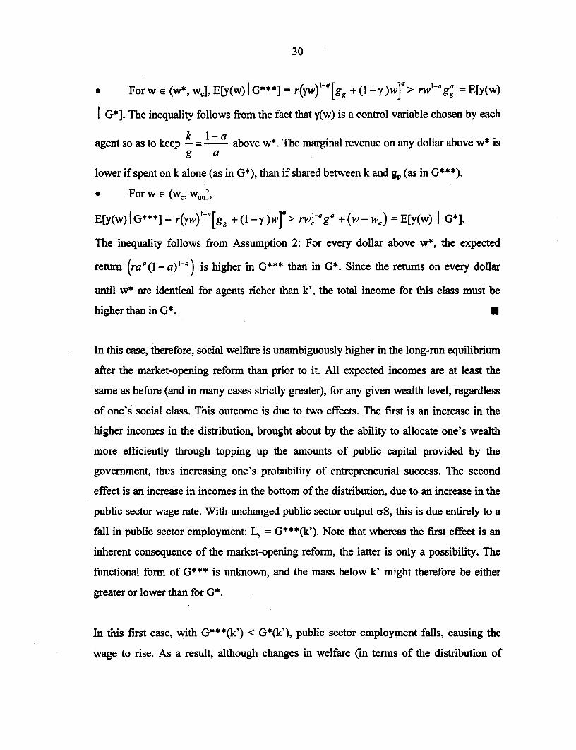
* For w E (w*, wj, E[y(w) I = r(yw) 1-a [gg + (1 - y )W] > rw Ia ga = E[y(w)

I G*]. The inequality follows from the fact that 7(w) is a control variable chosen by each

k I -aagent so as to keep - a above w*. The marginal revenue on any dollar above w* is

g alower if spent on k alone (as in G*), than if shared between k and gp (as in G***).

* For w E (wC, w%J,

E[y(w)IG***]= r(yw)-a [gg +(1-Y )W] > rw,..aga +(w-wc) =E[y(w) I G*].

The inequality follows from Assumption 2: For every dollar above w*, the expected

return (raa(l - a)'1a) is higher in G*** than in G*. Since the returns on every dollar

until w* are identical for agents richer than k', the total income for this class must be

higher than in G*. U

In this case, therefore, social welfare is unambiguously higher in the long-run equilibrium

after the market-opening reform than prior to it. All expected incomes are at least the

same as before (and in many cases strictly greater), for any given wealth level, regardless

of one's social class. This outcome is due to two effects. The first is an increase in the

higher incomes in the distribution, brought about by the ability to allocate one's wealth

more efficiently through topping up the amounts of public capital provided by the

government, thus increasing one's probability of entrepreneurial success. The second

effect is an increase in incomes in the bottom of the distribution, due to an increase in the

public sector wage rate. With unchanged public sector output aS, this is due entirely to a

fall in public sector employment: L, = G***(k'). Note that whereas the first effect is an

inherent consequence of the market-opening reform, the latter is only a possibility. The

functional form of G*** is unknown, and the mass below k' might therefore be either

greater or lower than for G*.

In this first case, with G***(k') < G*(k'), public sector employment falls, causing the

wage to rise. As a result, although changes in welfare (in terms of the distribution of

31

expected incomes) are unambiguous, the same can not be said of changes in inequality.

These will largely depend on the proportional rise in public sector wages, versus the

proportional rises in upper-class expected entrepreneurial incomes.

As noted above, however, the population mass below k' may also be greater in the post-

reform equilibrium than in the pre-reform equilibrium:

Proposition 6: If G***(k') > G*(k'), then (expected) income inequality between

representative agents of the three classes rises unambiguously between the pre-reform

equilibrium associated with G* and the post-reform equilibrium associated with G***.

Proof: Let the pre-reform equilibrium variables be denoted by the subscript 0, and the

post-reform equilibrium variables by the subscript 1. Let the representative agent of each

of the three classes be subscripted P, M and R, as in Section 3. The unambiguous rise in

inequality follows from a fall in the expected income of P, no change in the expected

income of M, and a rise in the expected income of R, as follows:

* E(ypl)=cJ,+w = ++W<G S +W=Wo0 +W=E(yPO)G (k') G *(kf)

* E(yMI) = rwlag' = E(yMO )

* E(yRI) = r(yw) a[gg +(1I-y)W]I > rw.-ago +(w-wC) = E(YRO)- (See the

proof of Proposition 5.) U

In this second case, merely because public sector employment increased, causing the

wage rate to fall, the beneficial impact of the market-opening reform appears substantially

less general. Only the (expanded) upper class sees rises in their expected incomes.

Inequality rises unambiguously between the three classes, and for any poverty line below

y(w*), poverty also rises. This can be interpreted as suggesting that the creation of private

suppliers of services previously provided only by the public sector, such as health care

and education, benefits only those who are rich enough to consider topping up the public

32

provision. Even though there is no requirement that a minimum amount of gp be

purchased, poorer agents do not benefit from the new markets, because they are either

precluded from employing its benefits in any production function at all, or because they

still choose to use all of their wealth to buy private capital. The only way in which these

new markets can help the poor is if they somehow reduce the mass of people constrained

to the public sector (G***(k')), perhaps through increased efficiency and reduced failure

rates in the private sector.

Figure 5 below illustrates the results from the last three propositions. The expected end-

of-period incomes are plotted on the upper panel, while expected marginal products are

plotted in the bottom panel. For agents with wealth between 0 and k', incomes are given

by the line segment AB, along the o + w line. When wealth reaches k', agents become

able to invest in the risky (but more profitable) private sector production function. There

is a discontinuity in the income function, and agents with wealth between k' and w* earn

incomes along the curve CD. At D, the marginal product of private capital (k) equals

ra!(1-a) -a, and hence the marginal product of public capital (g). With private markets for

gp available, as in G***, agents with wealth greater than w* share their wealth between k

and gp, so as to keep producing at the optimal input ratio k/g = (l-a)/a, and hence their

incomes are plotted along DE, until w.,, the upper bound of their ergodic set.19

In the pre-market-opening-reform equilibrium distribution G*, agents could not top up

the government transfers of g privately, so that they kept purchasing k until its expected

marginal product fell below 1, the return to simnply storing wealth. This happened at w¢,

so that middle-class expected incomes were then plotted along the arc CF. At F, agents

became saver/storers, in addition to the amount w, they invested in the private sector.

Their incomes were then plotted along FG. To understand propositions 5 and 6, note that

19 Note that k, rather than w, is on the x-axis. Beyond, w*, the amount of k purchased by agents (yw),which yields E(y) along DE, is strictly less than w. This is why, although DE is a line with slopegreater than one, there nevertheless exists an upper bound to the ergodic distribution. At w, so muchof w is spent on gp that the bequest left of the successful person's income is only the same as w,..

33

the curve CD is common to both income functions (whether under G* or G***). This is

the part of the middle class which remains middle class after the reforms, by virtue of not

being sufficiently rich to purchase privately supplied public capital. Above point D,

expected incomes are unambiguously greater in the post-reform equilibrium (DE lies

everywhere above DFG).

Figure S

E

E(y) rk

Ok' w~~~~ w~~, w~~ 0 + k

E[MPk]E[MPg]

E[MPg (gd]

ra(1-a)a 0 k' wk.............................................................

1 / . .~ ~ ~~~ E[MPk(gg)]

O k' w* WC WU W=U k

34

Proposition 5 refers to the case when the mass of people with wealth below k' in the

limiting distribution is lower in G*** than in the pre-reform equilibrium G*. Then, the

public sector wage rate o rises, shifting the AB segment up. In that case, it is easy to see

that no expected incomes in the post reform situation are lower than in the pre-reform

situation, for the same initial wealth level. This is what generates the unambiguous

increase in (expected) welfare described in Proposition 5. Inequality may or may not have

risen, depending on how much co rose by, compared to gains above w*.

Proposition 6, on the other hand, refers to the case when the mass of people with wealth

below k' in the limiting distribution is greater in G*** than in the pre-reform equilibrium

G*. Then, the public sector wage rate o falls, shifting the AB segment down. In that case,

incomes for the poorest class are lower in the post-reform equilibrium than before;

expected incomes for the (remaining) middle class are unchanged; and expected incomes

for the (enlarged) upper class are greater. Inequality between the classes rises

unambiguously.

T'he overall message from this section is that the creation of private markets for public

capital (e.g. education, health care, some infrastructure, telecommunications), which

enables investors to top up public provision by allocating resources to private purchases

of these services, contributes to economic efficiency but has ambiguous effects on

welfare. Efficiency gains are clear: even if public sector wages fall, public sector output is

unchanged, and there are always gains in the private sector. As for the distribution of

these gains, propositions 5 and 6 reveal that, while richer agents always gain, poorer

workers may either gain or lose, depending on what happens to public sector

employment. If their incomes decline, inequality in expected incomes will be

unambiguously higher in the post-reform long-run equilibrium. Even if their incomes

rise, but by proportionately less than those of the rich, some measures of inequality will

indicate an increase. This is an example of the sort of policy reforn likely to lead to more

efficient, but also more unequal, societies in the long run.

35

5. Returns to Skills and Volatility in the Labour Market

We have so far focused on the differential impacts of reforms - such as privatization or

market openings - on social classes characterized by their different occupational choices.

The model shed light on the mechanisms through which these transformations affected

people differently, depending on whether they worked for a safe but inefficient public

sector, or risked it out on their own as entrepreneurs in the new private sector. Within that

sector it was argued that, under plausible assumptions about the interaction between

public and private capital in the production function, expected returns differed depending

on whether one's wealth level allowed for purchases of privately provided education and

health care, say. The analysis of the model suggested circumstances under which

efficiency-augmenting policies, such as privatization or creating new markets, might lead

to increased inequality (and in some cases poverty), through lowering the incomes of

those unable to enter the private sector, or through increasing the incomes of the

wealthiest segment of the population disproportionately.

One important omission from this stylized model has been any treatment of the emerging

private sector labour market. Naturally, our treatment of the private sector as consisting

of atomistic household-firms should not be taken too literally; k can be interpreted as

private human capital and returns Ork could be seen as a wage rate which is linear in

human capital and subject to random employment shocks. Nevertheless, the focus of the

foregoing analysis was indeed on private physical wealth and its effect on broad

occupational choices and incomes, rather than on human capital and skills. This has

meant that we have largely ignored a third and important potential source of increased

inequality in economies in transition, namely an increase in the dispersion of labour

earnings due to changes in the pattern of returns to skills.

36

In particular, two changes are likely to have taken place in the earnings structure in these

economies: an increase in the returns to education at all levels of schooling, as the

artificially compressed wage structure under central planning is replaced by market

pricing for different types of labour; and an increase in the volatility of (real) pay,

reflecting reduced security in employment, greater risks of business failure, unpredictable

rates of inflation, etc. Both of these changes, which are essentially inherent in the greater

flexibility required of a functioning labour market, can lead to increased earnings

inequality even if there is no change at all in the underlying distribution of skills.

Consider the standard earnings functions often estimated in empirical studies of the

labour market:

logyj, = _ *logxi, + s j, (16)

where yi, denotes the earnings of individual i in period t; x is a vector of individual

characteristics, such as years of schooling, years of experience, gender, race, etc; £ is a

stochastic term; and the parameter pi in vector J can be interpreted as the "earnings

elasticity" of characteristic xi, providing some indication of its labour market return.

In order to focus more narrowly on returns to skills, suppose the true earnings

determination model in our transition economy is given simply by:

logy1, = J3, logsi, + logO j, (17)

where sit denotes some measure of the level of skills" embodied in individual i at time t,

and e =logO, - i.d. N(O,a 2,). Let us also assume that this transitional society is

characterized by a lognormal distribution of skills, so that log si - N(11 ,a 2 ). Let log 0

and log s be distributed independently of any current or lagged value of each other. log 0

is also distributed independently of its own lagged values, but need not be identically

distributed over time. P is a constant across individuals i, and is determined exogenously

at each time t.

20 This could be a standard proxy such as years of formal schooling, or a more complex indicator,incorporating years of experience and/or quality adjustments.

37

Equation (17) can then be rewritten as yj, =0 ,,sP, with s LN( and

0- LN(O,ai, ). Being the product of two lognormals, it follows that earnings are also

distributed lognormally, as follows:

Yit a LN(,ps,p,2aC + f,) (18)

It is then immediate to see how the two transformations discussed above impact the

distribution. First, an increase in the education elasticity of earnings P (the 'returns to

education') will raise both the mean and the dispersion of the earnings distribution. Mean

eamings rise, since the return on the mean level of education has risen. But a rise in , will

also increase the variance of the lognormal distribution of earnings, even if there has been

no change in the variance of the underlying distribution of skills (a 2 ). As one would

expect, the move from a compressed earnings-education profile under central planning to

a steeper one in a freer labour market contributes to a further skewing of the earnings

distribution.

A second mechanism through which transition to a freer labour market may lead to

increases in the dispersion of the earnings distribution is a decline in the 'security' of an

individual's earnings, arising from an increase in volatility. There is some riskiness

associated with one's earnings under any situation, which is embodied in the stochastic

term cit in equation (16) (or Oit in equation 17). This term captures shocks such as

illnesses, unemployment, bankruptcy of one's employers, bad weather, poor harvests,

recessions, etc. It is reasonable to suppose that the variance of these shocks, at ,, is higher

in a market economy than under central planning. In the former, unemployment is more

widespread; earnings are more responsive to macroeconomic shocks; firms go bankrupt

(and start up) more often; business deals fail astoundingly (or succeed explosively) more

often than in the latter. Greater efficiency comes at the cost of greater volatility, higher

risk. Ceteris paribus, a higher variance for the stochastic term so, means a greater

variance for the earnings distribution. Combined with an increase in the returns to

38

education (,B), this suggests that the transformations in the structure of earnings likely to

be associated with the labour market transition from central planning will lead to an

increase in the dispersion of the distribution of earnings. This adds another mechanism to

those considered in Sections 3 and 4, through which economic reforms associated with

the process of economic transition can increase income inequality, despite their beneficial

(long-term) effects on efficiency.

6. Conclusions.

This paper investigates ways in which some of the economic transformations associated

with transition from central planning to a market system affect the distribution of income.

Most of the analysis relies on a dynamic model of wealth distribution and occupational

choice, in which agents choose between working for a deterministic wage in a (relatively

inefficient) public sector and being entrepreneurs in a risky private sector, where the

probability of success increases with the availability of public capital. Credit markets are

assumed to be (extremely) imperfect, and there is a minimum scale of production

required for participation in the private sector. The model yields a steady-state wealth

distribution in which the poorest agents are unable to invest in the private sector, and are

constrained to safe but low-paying public sector employment. Richer agents invest in the

new, risky private sector and can be further divided between a middle-class, where people

exhaust their initial wealth in production, and an upper class, where some wealth is

(risklessly) stored, in addition to the private sector investments.

The effects of a privatization of some of the government's productive assets on the

expected incomes of households differ along this wealth distribution. As a result, even if

privatization is designed to be equitable, with assets uniformly distributed through

vouchers amongst the population, it turns out that inequality may rise both in the short

and in the long run. In the short run, the middle and upper classes stand to gain

unambiguously, since they are able to channel the extra capital they receive from the

39

government into their own private production functions, increasing their expected returns.

The impact on the welfare of the poor is more complex, since the privatization is likely to

affect the public sector wage rate, from which they derive most of their incomes. If wages

are set to equal the public sector average product of labour, a reduction in its capital stock

which exceeds any reduction in public employment will lower the wage, and this effect

may be sufficient to outweigh short-term gains from the receipt of a privatization

voucher. If barriers to entry into the new private sector are large, and privatization fails to

move a substantial number of public employees to alternative, more productive

occupations, then the decline in the public sector wage rate will lead to greater inequality

and deeper poverty in the transition economy. If the transfer of labour to alternative

occupations outside the public sector continues to be insufficient in the long run, so that

the new equilibrium is characterized by a government which has lost more capital than it

has shed workers, it is likely that the new steady-state will also be characterized by

greater inequality and poverty (for at least some poverty lines).

Another transformation which is likely to increase economic efficiency but also lead to

greater inequality is the creation of markets where private sector entrepreneurs can buy

and sell substitutes to 'public capital' goods, such as education and health services, toll

roads, etc. Whilst this transformation will not hurt the poor - unless it somehow leads to

an increase in public sector employment - it is very likely to benefit the rich much more

than the poor. This is because only richer agents will find it worthwhile to channel their

private resources to pay for extra (or better) schools, health insurance and cellular

telecommunications, rather than investing it in straight-forward private capital. As a

result, though, the expected returns from their investments rise, and the distance between

their incomes and those of the remaining middle class and the poor increases. Once again,

the increase in inequality will be the smaller, the greater the impact of the reform in terms

of enabling people to escape public employment into a more productive private sector

occupation.

40

Finally, substantial changes taking place in the labour market are certain to affect the

distribution of final incomes in transition economies. While we did not model the private

sector labour market explicitly, a simple earnings equation was used to suggest that an

increase in the slope of the earnings-education profile - due presumably to a

"decompression" of the wage structure prevalent under central planning - will increase

the dispersion of the earnings distribution, even if the underlying distribution of skills has

not changed. This effect may be compounded by an increase in the volatility of earnings,

due perhaps to greater risks of unemployment or business failures in a market economy.

A greater variance in the probability distribution of any such random shock will also

increase the variance in the cross-section distribution of earnings.

Overall, the analysis illustrated a number of specific mechanisms through which policies

and developments which increase economic efficiency (measured by equilibrium

economy-wide output) are likely to lead to greater inequality and, in some cases, higher

poverty. These results may attain even in the long run, with new limiting (steady-state)

distributions characterized by greater inequality than prior to the transition. Whenever the

incomes accruing to the poor actually decline, while average incomes rise, there is a

classic equity-efficiency trade-off. In those cases, greater efficiency does not

automatically imply higher social welfare, and policy implications depend on a normative

judgement.

Given how inefficient systems based on state ownership and central planning turned out

to be, the question will almost certainly not be whether these efficiency-augmenting

reforms should take place, but how. The general lesson that can be derived from this

paper is that - since economic reform takes place in the context 'f an existing non-

degenerate wealth distribution, and with incomplete and imperfect markets - explicit

attention should be paid to equity objectives. Greater efficiency is not sufficient to imply

higher social welfare. In particular, reformers should seek to ensure three things: that the

state continues to produce goods and services in which market failures outweigh

government failures - such as law and order, primary education, basic health care, rural

41

infrastructure - and which are in many cases indispensable to a successful private sector;

that new profitable opportunities in the private sector are available to poor people too,

enabling them to leave the inefficient segments of the old public sector and to benefit

from the greater prosperity to be achieved elsewhere; and that provisions exist to protect

minimum standards of welfare for the poorest people. The ergodic nature of this model's

limiting distribution is a reminder that, over the long-run, all lineages face a positive

probability of finding themselves among the poor, and thus benefit from whatever safety

nets have been put in place to provide them with a minimum income and a chance for

subsequent upward mobility. The market economy is an inherently risky system; by

replacing the public sector employer of last resort with suitable altemative safety nets,

today's reformers may be looking after the welfare of their grandchildren's children.

42

Append&x

Proof of Lemma 1: By contradiction. Suppose E[MPk(w.)] >1. Then the third class

defined in proposition 1 would not exist, since all agents in the ergodic distribution would

invest all their initial wealth in production function (2). Then, rather than setting wt+ = wt

in w, 1 = (1 -aXl -t)[rwc + (w, - wj)], which yields (10), we would search for an

upper bound by setting wt+l = wt in w,,1 = (1 - a)(I - X )[rw, ], the only solution to which

is w = 0, implying the inexistence of an ergodic set. If an ergodic set exists, its upper

bound exceeds any wealth level such that E[MPk(w)] > 1 . Since E[MPk] < O, Vk, itak

follows that E[MPk(w.)] <1.E0

43

References.

Aghion, P. and P. Bolton (1997): "A Theory of Trickle-Down Growth andDevelopment", Review of Economic Studies, 64, pp.151-172 .

Andreoni, J. (1989): "Giving with Impure Altruism: applications to charity and Ricardianequivalence", Journal of Political Economy, 97, pp.14 4 7 -1 4 5 8 .

Arrow, K.J. (1962): "The Economic Implications of Learning by Doing", Review ofEconomic Studies, 29, pp.15 5-1 7 3 .

Atkinson, A.B. and J. Micklewright (1992): Economic Transformation in Eastern Europeand the Distribution of Income, (Cambridge: Cambridge University Press).

Banerjee, A.V. and A.F. Newman (1991): "Risk Bearing and the Theory of IncomeDistribution", Review of Economic Studies, 58, pp.2 1 1-235.

Banerjee, A.V. and A.F. Newman (1993): "Occupational Choice and the Process ofDevelopment", Journal of Political Economy, 101, No.2, pp.2 7 4 -29 8 .

Barro, R.J. (1990): "Government Spending in a Simple Model of Endogenous Growth",Journal of Political Economy, 98, No.5, pt.2, pp.S103-S125.

B6nabou, R. (1996): "Unequal Societies", NBER Working Paper 5583 (May).

Commander, S. and F. Coricelli (1995): Unemployment, Restructuring, and the LabourMarket in Eastern Europe and Russia, (Washington, DC: The World Bank).

Deininger, K. and L. Squire (1996): "A New Data Set Measuring Income Inequality",World Bank Economic Review, 10, pp.5 6 5 -5 9 1.

EBRD (1995): Transition Report 1995, (London: European Bank for Reconstruction andDevelopment).

Ferreira, F.H.G. (1995): "Roads to Equality: Wealth Distribution Dynamics with Public-Private Capital Complementarity", LSE-STICERD Discussion Paper TE/95/286(London).

Ferreira, F.H.G. (1996): "Structural Adjustment, Income Distribution and the Role ofGovernment: theory, and evidence from Brazil", PhD dissertation, LSE (London).

Ferreira, F.H.G. and J.A. Litchfield (1997): "Education or Inflation: the roles of structuralfactors and macroeconomic instability in explaining Brazilian inequality in the 1980s",LSE-STICERD DARP Discussion Paper (forthcoming).

44

Galor, 0. and J. Zeira (1993): "Income Distribution and Macroeconomics", Review ofEconomic Studies, 60, pp.35-52.

Milanovic, B. (1997, forthcoming): Income, Inequality and Poverty During theTransition, (Washington, DC: The World Bank).

Piketty, T. (1997): "The Dynamics of the Wealth Distribution and the Interest Rate withCredit Rationing", Review of Economic Studies, 64, pp.173 -1 8 9 .

Romer, P.M. (1986): "Increasing Returns and Long-Run Growth", Journal of PoliticalEconomy, 94, pp.1002-1037.

Stem, N.H. (1991): "The Determinants of Growth", Economic Journal, 101, pp.122-133.

World Bank (1996): Poverty Reduction and the World Bank: progress and challenges inthe 1990s, (Washington, DC: The World Bank).

Policy Research Working Paper Series

ContactTitle Author Date for paper

WPS1787 Trading Arrangements and Diego Puga June 1997 J. NgaineIndustrial Development Anthony J. Venables 37947

WPS1788 An Economic Analysis of Woodfuel Kenneth M. Chomitz June 1997 A. MaranonManagement in the Sahel: The Case Charles Griffiths 39074of Chad

WPS1789 Competition Law in Bulgaria After Bernard Hoekman June 1997 J. NgaineCentral Planning Simeon Djankov 37947

WPS1790 Interpreting the Coefficient of Barry R. Chiswick June 1997 P. SinghSchooling in the Human Capital 85631Earnings Function

WPS1791 Toward Better Regulation of Private Hemant Shah June 1997 N. JohlPension Funds 38613

WPS1792 Tradeoffs from Hedging: Oil Price Sudhakar Satyanarayan June 1997 E. SomensattoRisk in Ecuador 30128

WPS1793 Wage and Pension Pressure on the Alain de Crombrugghe June 1997 M. JanduPolish Budget 33103

WPS1794 Ownership Structure, Corporate Xiaonian Xu June 1997 J. ChinsenGovernance, and Corporate Yan Wang 34022Performance: The Case of ChineseStock Companies

WPS1795 What Educational Production Lant Pritchett July 1997 S. FallonFunctions Really Show: A Positive Deon Filmer 38009Theory of Education Spending

WPS1796 Cents and Sociability: Household Deepa Narayan July 1997 S. FallonIncome and Social Capital in Rural Lant Pritchett 38009Tanzania

WPS1 797 Formal and Informal Regulation Sheoli Pargal July 1997 E. de Castroof Industrial Pollution: Hemamala Hettige 89121Comparative Evidence from Manjula SinghIndonesia and the United States David Wheeler

WPS1798 Poor Areas, Or Only Poor People? Martin Ravallion July 1997 P. SaderQuentin Wodon 33902

WPS1799 More for the Poor Is Less for the Jonath B. Gelbach July 1997 S. FallonPoor: The Politics of Targeting Lant H. Pritchett 38009

WPS1 800 Single-Equation Estimation of the John Baffes August 1997 P. KokilaEquilibrium Real Exchange Rate Ibrahim A. Elbadawi 33716

Stephen A. O'Connell

Policy Research Working Paper Series

ContactTitle Author Date for paper

WPS1801 Regional Integration as Diplomacy Maurice Schiff August 1997 J. NgaineL. Alan Winters 37947

WPS1802 Are There Synergies Between Harry Huizinga August 1997 P. Sintim-AboagyeWorld Bank Partial Credit 38526Guarantees and Private Lending?

WPS1803 Fiscal Adjustments in Transition Barbara Fakin August 1997 M. JanduEconomies: Social Transfers and the Alain de Crombrugghe 33103Efficienoy of Public Spending: AComparison with OECD Countries

WPS1804 Financial Sector Adjustment Lending: Robert J. Cull August 1997 P. Sintim-AboagyeA Mid-Course Analysis 37644

WPS1 805 Regional Economic Integration and Junichi Goto August 1997 G. IlogonAgricultural Trade 33732

WPS1806 An International Statistical Survey Salvatore Schiavo-Campo August 1997 M. Gueverraof Government Employment and Giulio de Tommaso 32959Wages Amitabah Mukherjee

WPS1807 The Ghosts of Financing Gap: William Easterly August 1997 K. LabrieHow the Harrod-Domar Growth 31001Model Still Haunts DevelopmentEconomics