AP Calculus AB/BC Formula and Concept Cheat Sheet

Limit of a Continuous Function

If f(x) is a continuous function for all real numbers, then lim𝑥→𝑐

𝑓(𝑥) = 𝑓(𝑐)

Limits of Rational Functions

A. If f(x) is a rational function given by 𝑓(𝑥) =𝑝(𝑥)

𝑞(𝑥) ,such that 𝑝(𝑥) and 𝑞(𝑥) have no common factors, and c is a real

number such that 𝑞(𝑐) = 0, then

I. lim𝑥→𝑐

𝑓(𝑥) does not exist

II. lim𝑥→𝑐

𝑓(𝑥) = ±∞ x = c is a vertical asymptote

B. If f(x) is a rational function given by 𝑓(𝑥) =𝑝(𝑥)

𝑞(𝑥), such that reducing a common factor between 𝑝(𝑥) and 𝑞(𝑥) results

in the agreeable function k(x), then

lim𝑥→𝑐

𝑓(𝑥) = lim𝑥→𝑐

𝑝(𝑥)

𝑞(𝑥)= lim

𝑥→𝑐 𝑘(𝑥) = 𝑘(𝑐) Hole at the point (𝑐, 𝑘(𝑐))

Limits of a Function as x Approaches Infinity

If f(x) is a rational function given by (𝑥) =𝑝(𝑥)

𝑞(𝑥) , such that 𝑝(𝑥) and 𝑞(𝑥) are both polynomial functions, then

A. If the degree of p(x) > q(x), lim𝑥→∞

𝑓(𝑥) = ∞

B. If the degree of p(x) < q(x), lim𝑥→∞

𝑓(𝑥) = 0 y = 0 is a horizontal asymptote

C. If the degree of p(x) = q(x), lim𝑥→∞

𝑓(𝑥) = 𝑐, where c is the ratio of the leading coefficients.

y = c is a horizontal asymptote

Special Trig Limits

A. lim𝑥→0

sin 𝑎𝑥

𝑎𝑥= 1 B. lim

𝑥→0

𝑎𝑥

sin 𝑎𝑥= 1 C. lim

𝑥→0

1−cos 𝑎𝑥

𝑎𝑥= 0

L’Hospital’s Rule

If results lim𝑥→𝑐

𝑓(𝑥) or lim𝑥→∞

𝑓(𝑥) results in an indeterminate form ( 0

0 ,

∞

∞ , ∞ − ∞ , 0 ∙ ∞ , 00 , 1∞ , ∞0) , and

𝑓(𝑥) =𝑝(𝑥)

𝑞(𝑥) , then

lim𝑥→𝑐

𝑓(𝑥) = lim𝑥→𝑐

𝑝(𝑥)

𝑞(𝑥)= lim

𝑥→𝑐

𝑝′(𝑥)

𝑞′(𝑥) and lim

𝑥→∞𝑓(𝑥) = lim

𝑥→∞

𝑝(𝑥)

𝑞(𝑥)= lim

𝑥→∞

𝑝′(𝑥)

𝑞′(𝑥)

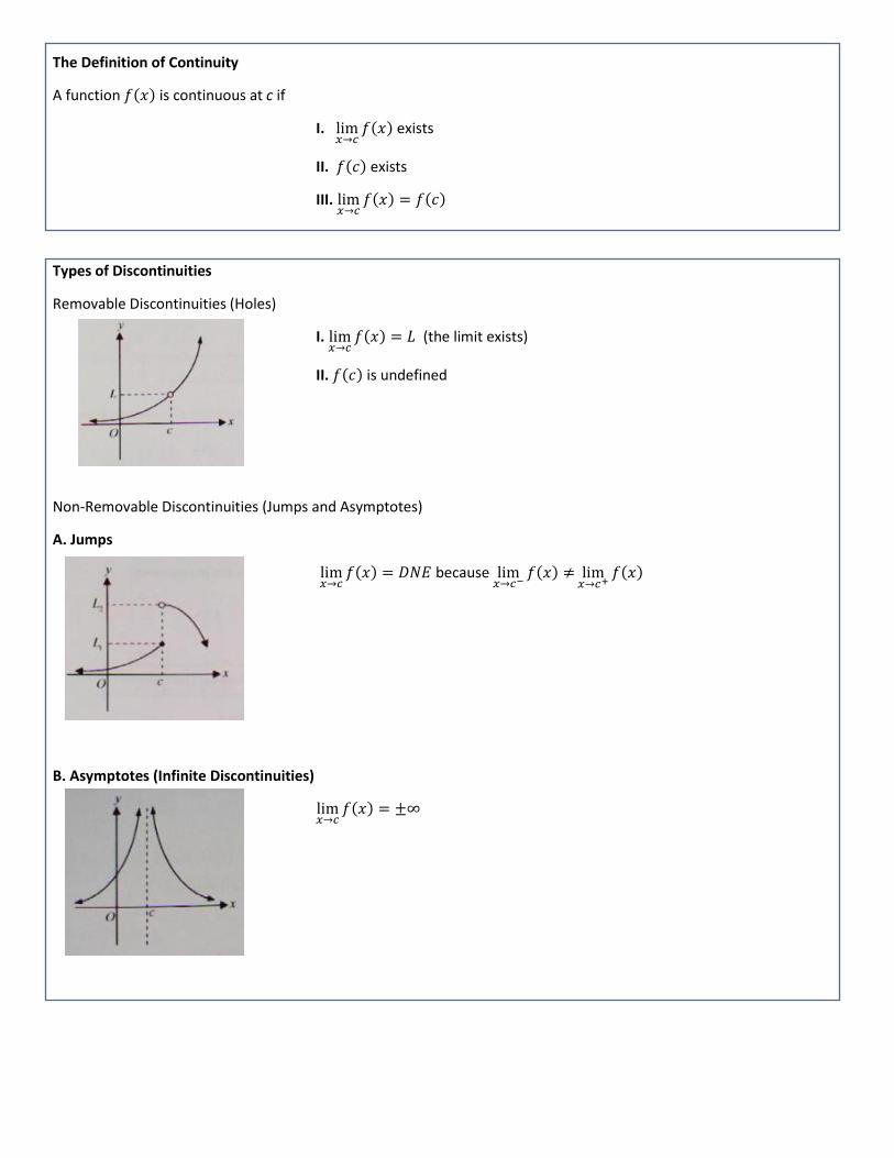
The Definition of Continuity

A function 𝑓(𝑥) is continuous at c if

I. lim𝑥→𝑐

𝑓(𝑥) exists

II. 𝑓(𝑐) exists

III. lim𝑥→𝑐

𝑓(𝑥) = 𝑓(𝑐)

Types of Discontinuities

Removable Discontinuities (Holes)

I. lim𝑥→𝑐

𝑓(𝑥) = 𝐿 (the limit exists)

II. 𝑓(𝑐) is undefined

Non-Removable Discontinuities (Jumps and Asymptotes)

A. Jumps

lim𝑥→𝑐

𝑓(𝑥) = 𝐷𝑁𝐸 because lim𝑥→𝑐−

𝑓(𝑥) ≠ lim𝑥→𝑐+

𝑓(𝑥)

B. Asymptotes (Infinite Discontinuities)

lim𝑥→𝑐

𝑓(𝑥) = ±∞

Intermediate Value Theorem

If f is a continuous function on the closed interval [a, b] and k is any number between f(a) and f(b), then there exists at

least one value of c on [a, b] such that f(c) = k. In other words, on a continuous function, if f(a)< f(b), any y – value

greater than f(a) and less than f(b) is guaranteed to exists on the function f.

Average Rate of Change

The average rate of change, m, of a function f on the interval [a, b] is given by the slope of the secant line.

𝑚 =𝑓(𝑏)−𝑓(𝑎)

𝑏−𝑎

Definition of the Derivative

The derivative of the function f, or instantaneous rate of change, is given by converting the slope of the secant line to

the slope of the tangent line by making the change is x, Δx or h, approach zero.

𝑓′(𝑥) = limℎ→0

𝑓(𝑥+ℎ)−𝑓(𝑥)

ℎ

Alternate Definition

𝑓′(𝑐) = lim𝑥→𝑐

𝑓(𝑥)−𝑓(𝑐)

𝑥−𝑐

Differentiability and Continuity Properties

A. If f(x) is differentiable at x = c, then f(x) is continuous at x = c.

B. If f(x) is not continuous at x = c, then f(x) is not differentiable at x = c.

C. The graph of f is continuous, but not differentiable at x = c if:

I. The graph has a cusp or sharp point at x = c

II. The graph has a vertical tangent line at x = c

III. The graph has an endpoint at x = c

Basic Derivative Rules

Given c is a constant,

Derivatives of Trig Functions

Derivatives of Inverse Trig Functions

Derivatives of Exponential and Logarithmic Functions

Explicit and Implicit Differentiation

A. Explicit Functions: Function y is written only in terms of the variable x (𝑦 = 𝑓(𝑥)). Apply derivatives rules normally.

B. Implicit Differentiation: An expression representing the graph of a curve in terms of both variables x and y.

I. Differentiate both sides of the equation with respect to x. (terms with x

differentiate normally, terms with y are multiplied by 𝑑𝑦

𝑑𝑥 per the chain rule)

II. Group all terms with 𝑑𝑦

𝑑𝑥 on one side of the equation and all other terms on

the other side of the equation.

III. Factor 𝑑𝑦

𝑑𝑥 and express

𝑑𝑦

𝑑𝑥 in terms of x and y.

Tangent Lines and Normal Lines

A. The equation of the tangent line at a point (𝑎, 𝑓(𝑎)): 𝑦 − 𝑓(𝑎) = 𝑓′(𝑎)(𝑥 − 𝑎)

B. The equation of the normal line at a point (𝑎, 𝑓(𝑎)): 𝑦 − 𝑓(𝑎) = −1

𝑓′(𝑎)(𝑥 − 𝑎)

Mean Value Theorem for Derivatives

If the function f is continuous on the close interval [a, b] and differentiable on the open interval (a, b), then there exists

at least one number c between a and b such that

𝑓′(𝑐) =𝑓(𝑏)−𝑓(𝑎)

𝑏−𝑎 The slope of the tangent line is equal to the slope of the secant line.

Rolle’s Theorem (Special Case of Mean Value Theorem)

If the function f is continuous on the close interval [a, b] and differentiable on the open interval (a, b), and f(a) = f(b),

then there exists at least one number c between a and b such that

𝑓′(𝑐) =𝑓(𝑏)−𝑓(𝑎)

𝑏−𝑎= 0

Particle Motion

A velocity function is found by taking the derivative of position. An acceleration function is found by taking the

derivative of a velocity function.

𝑥(𝑡) Position

𝑥′(𝑡) = 𝑣(𝑡) Velocity * |𝑣(𝑡)| = 𝑠𝑝𝑒𝑒𝑑

𝑥′′(𝑡) = 𝑣′(𝑡) = 𝑎(𝑡) Accleration

Rules:

A. If velocity is positive, the particle is moving right or up. If velocity is negative, the particle is moving left or down.

B. If velocity and acceleration have the same sign, the particle speed is increasing. If velocity and acceleration have

opposite signs, speed is decreasing.

C. If velocity is zero and the sign of velocity changes, the particle changes direction.

Related Rates

A. Identify the known variables, including their rates of change and the rate of change that is to be found. Construct an

equation relating the quantities whose rates of change are known and the rate of change to be found.

B. Implicitly differentiate both sides of the equation with respect to time. (Remember: DO NOT substitute the value of a

variable that changes throughout the situation before you differentiate. If the value is constant, you can substitute it

into the equation to simplify the derivative calculation).

C. Substitute the known rates of change and the known values of the variables into the equation. Then solve for the

required rate of change.

*Keep in mind, the variables present can be related in different ways which often involves the use of similar

geometric shapes, Pythagorean Theorem, etc.

Extrema of a Function

A. Absolute Extrema: An absolute maximum is the highest y – value of a function on a given interval or across the entire

domain. An absolute minimum is the lowest y – value of a function on a given interval or across the entire domain.

B. Relative Extrema

I. Relative Maximum: The y-value of a function where the graph of the function changes from increasing

to decreasing. Another way to define a relative maximum is the y-value where derivative of a function

changes from positive to negative.

II. Relative Minimum: The y-value of a function where the graph of the function changes from

decreasing to increasing. Another way to define a relative maximum is the y-value where derivative of a

function changes from negative to positive.

Critical Value

When f(c) is defined, if f ‘ (c) = 0 or f ‘ is undefined at x = c, the values of the x – coordinate at those points are called

critical values.

*If f(x) has a relative extrema at x = c, then c is a critical value of f.

Extreme Value Theorem

If the function f continuous on the closed interval [a, b], then the absolute extrema of the function f on the closed

interval will occur at the endpoints or critical values of f.

*After identifying critical values, create a table with endpoints and critical values. Calculate the y – value at each

of these x values to identify the extrema.

Increasing and Decreasing Functions

For a differentiable function f

A. If 𝑓′(𝑥) > 0 in (a, b), then f is increasing on (a, b) Tangent line has a positive slope

B. If 𝑓′(𝑥) < 0 in (a, b), then f is decreasing on (a, b) Tangent line has a negative slope

C. If 𝑓′(𝑥) = 0 in (a, b), then f is constant on (a, b) Tangent line has a zero slope (horizontal)

First Derivative Test

After calculating any discontinuities of a function f and calculating the critical values of a function f, create a sign chart for f ‘, reflecting the domain, discontinuities, and critical values of a function f.

A. If 𝑓′(𝑥) changes sign from negative to positive at 𝑥 = 𝑐, then 𝑓(𝑐) is a relative minimum of f.

B. If 𝑓′(𝑥) changes sign from positive to negative at 𝑥 = 𝑐, then 𝑓(𝑐) is a relative maximum of f.

*If there is no sign change of 𝑓′(𝑥), there exists a shelf point

Concavity

For a differentiable function f(x),

A. If 𝑓′′(𝑥) > 0, the graph of 𝑓(𝑥) is concave up

This means 𝑓′(𝑥) is increasing

B. If 𝑓′′(𝑥) < 0, the graph of 𝑓(𝑥) is concave down

This means 𝑓′(𝑥) is decreasing

Second Derivative Test

For a function f(x) that is continuous at x = c

A. If 𝑓′(𝑐) = 0 and 𝑓′′(𝑐) > 0, then 𝑓(𝑐) is a relative minimum.

B. If 𝑓′(𝑐) = 0 and 𝑓′′(𝑐) < 0, then 𝑓(𝑐) is a relative maximum.

* If 𝑓′(𝑐) = 0 and 𝑓′′(𝑐) = 0, you must use the first derivative test to determine extrema

BC Only: Derivatives of Parametric Functions

If f and g are continuous functions of t on an interval, then the equations 𝑥 = 𝑓(𝑡) and 𝑦 = 𝑔(𝑡) are called

parametric equations, providing the position in the coordinate plane, and t is called the parameter.

A. The slope of the curve at the point (x, y) is

𝑑𝑦

𝑑𝑥=

𝑑𝑦/𝑑𝑡

𝑑𝑥/𝑑𝑡 , provided 𝑑𝑥/𝑑𝑡 ≠ 0

B. The second derivative at the point (x, y) is

𝑑2𝑦

𝑑𝑥2=

𝑑𝑑𝑡

(𝑑𝑦𝑑𝑥

)

𝑑𝑥𝑑𝑡

Point of Inflection

Let f be a functions whose second derivative exists on any interval. If f is continuous at x = c, f ‘’(c) = 0 or f ‘’(c) is

undefined, and f ‘’(x) changes sign at x = c, then the point (𝑐, 𝑓(𝑐)) is a point of inflection.

Optimization

Finding the largest or smallest value of a function subject to some kind of constraints.

A. Define the primary equation for the quantity to be maximized or minimized. Define a feasible domain for the

variables present in the equation.

B. If necessary, define a secondary equation that relates the variables present in the primary equation. Solve this

equation for one of the variables and substitute into the primary equation.

C. Once the primary equation is represented in a single variable, take the derivative of the primary equation.

D. Find the critical values using the derivative calculated.

E. The optimal solution will more than likely be found at a critical value from D. Keep in mind, if the critical values do not

represent a minimum or a maximum, the optimal solution may be found at an endpoint of the feasible domain.

Derivative of an Inverse

If f and its inverse g are differentiable, and the point (c, f(c)) exists on the function f meaning the point (f(c), c) exists on

the function g¸ then 𝑑

𝑑𝑥[𝑔(𝑥)] =

1

𝑓′(𝑓−1(𝑥))=

1

𝑓′(𝑓(𝑐))

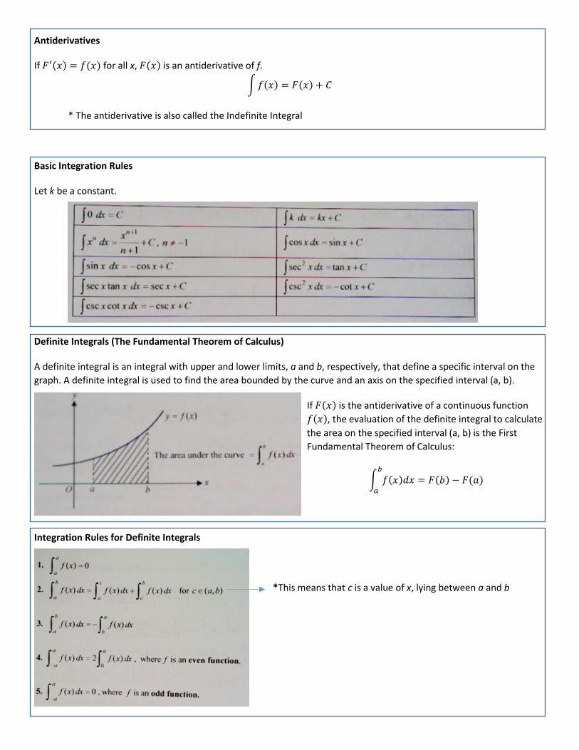
Antiderivatives

If 𝐹′(𝑥) = 𝑓(𝑥) for all x, 𝐹(𝑥) is an antiderivative of f.

∫ 𝑓(𝑥) = 𝐹(𝑥) + 𝐶

* The antiderivative is also called the Indefinite Integral

Basic Integration Rules

Let k be a constant.

Definite Integrals (The Fundamental Theorem of Calculus)

A definite integral is an integral with upper and lower limits, a and b, respectively, that define a specific interval on the

graph. A definite integral is used to find the area bounded by the curve and an axis on the specified interval (a, b).

If 𝐹(𝑥) is the antiderivative of a continuous function

𝑓(𝑥), the evaluation of the definite integral to calculate

the area on the specified interval (a, b) is the First

Fundamental Theorem of Calculus:

∫ 𝑓(𝑥)𝑑𝑥 = 𝐹(𝑏) − 𝐹(𝑎)𝑏

𝑎

Integration Rules for Definite Integrals

*This means that c is a value of x, lying between a and b

Riemann Sum (Approximations)

A Riemann Sum is the use of geometric shapes (rectangles and trapezoids) to approximate the area under a curve,

therefore approximating the value of a definite integral.

If the interval [a, b] is partitioned into n subintervals, then each subinterval, Δx, has a width: ∆𝑥 =𝑏−𝑎

𝑛.

Therefore, you find the sum of the geometric shapes, which approximates the area by the following formulas:

A. Right Riemann Sum

𝐴𝑟𝑒𝑎 ≈ ∆𝑥 [𝑓(𝑥0) + 𝑓(𝑥1) + 𝑓(𝑥2) + ⋯ + 𝑓(𝑥𝑛−1)]

B. Left Riemann Sum

𝐴𝑟𝑒𝑎 ≈ ∆𝑥 [𝑓(𝑥1) + 𝑓(𝑥2) + 𝑓(𝑥3) + ⋯ + 𝑓(𝑥𝑛)]

C. Midpoint Riemann Sum

𝐴𝑟𝑒𝑎 ≈ ∆𝑥 [𝑓(𝑥1/2) + 𝑓(𝑥3/2) + 𝑓(𝑥5/2) + ⋯ + 𝑓(𝑥(2𝑛−1)/2)]

D. Trapezoidal Sum

𝐴𝑟𝑒𝑎 ≈1

2 ∆𝑥 [𝑓(𝑥0) + 2 𝑓(𝑥1) + 2 𝑓(𝑥2) + ⋯ + 2𝑓(𝑥𝑛−1) + 𝑓(𝑥𝑛)]

Properties of Riemann Sums

A. The area under the curve is under approximated when

I.A Left Riemann sum is used on an increasing function.

II. A Right Riemann sum is used on a decreasing function.

III. A Trapezoidal sum is used on a concave down function.

B. The area under the curve is over approximated when

I.A Left Riemann sum is used on a decreasing function.

II. A Right Riemann sum is used on an increasing function.

III. A Trapezoidal sum is used on a concave up function.

Riemann Sum (Limit Definition of Area)

Let f be a continuous function on the interval [a, b]. The area of the region bounded by the graph of the function f and

the x – axis (i.e. the value of the definite integral) can be found using

∫ 𝑓(𝑥)𝑑𝑥𝑏

𝑎

= lim𝑛→∞

∑ 𝑓(𝑐𝑖) ∆𝑥

𝑛

𝑖=1

Where 𝑐𝑖 is either the left endpoint (𝑐𝑖 = 𝑎 + (𝑖 − 1)∆𝑥) or right endpoint (𝑐𝑖 = 𝑎 + 𝑖∆𝑥) and ∆𝑥 = (𝑏 − 𝑎)/𝑛.

Average Value of a Function

If a function f is continuous on the interval [a, b], the average value of that function f is given by

1

𝑏 − 𝑎∫ 𝑓(𝑥)𝑑𝑥

𝑏

𝑎

Second Fundamental Theorem of Calculus

If a function f is continuous on the interval [a, b], let 𝑢 represent a function of x, then

𝐀. 𝑑

𝑑𝑥[∫ 𝑓(𝑡)𝑑𝑡

𝑥

𝑎

] = 𝑓(𝑥)

𝐁. 𝑑

𝑑𝑥[∫ 𝑓(𝑡)𝑑𝑡

𝑏

𝑥

] = −𝑓(𝑥)

𝐂. 𝑑

𝑑𝑥[∫ 𝑓(𝑡)𝑑𝑡

𝑢(𝑥)

𝑎

] = 𝑓(𝑢(𝑥)) ∙ 𝑢′(𝑥)

Integration of Exponential and Logarithmic Formulas

BC Only: Integration by Parts

If u and v are differentiable functions of x, then

∫ 𝑢 𝑑𝑣 = 𝑢𝑣 − ∫ 𝑣 𝑑𝑢

Tips: For your choice of the function u, make the selection following:

A. LIPET: Logarithmic, Inverse Trig, Polynomial, Exponential, Trig

B. LIATE: Logarithmic, Inverse Trig, Algebraic, Trig, Exponential

∗ Comes from Integration by Parts. MEMORIZE ∫ ln 𝑥 𝑑𝑥 = 𝑥 ln 𝑥 − 𝑥 + 𝐶

Integration of Trig and Inverse Trig

BC Only: Partial Fractions

Let R(x) represent a rational function of the form 𝑅(𝑥) =𝑁(𝑥)

𝐷(𝑥). If D(x) is a factorable polynomial, Partial Fractions can

be used to rewrite R(x) as the sum or difference of simpler rational functions. Then, integration using natural log.

A. Constant Numerator

B. Polynomial Numerator

BC Only: Improper Integrals

An improper integral is characterized by having a limits of integration that is infinite or the function f having an

infinite discontinuity (asymptote) on the interval [a, b].

A. Infinite Upper Limit (continuous function)

∫ 𝑓(𝑥)𝑑𝑥∞

𝑎

= lim𝑏→∞

∫ 𝑓(𝑥)𝑑𝑥𝑏

𝑎

B. Infinite Lower Limit (continuous function)

∫ 𝑓(𝑥)𝑑𝑥𝑏

−∞

= lim𝑎→−∞

∫ 𝑓(𝑥)𝑑𝑥𝑏

𝑎

C. Both Infinite Limits (continuous function)

∫ 𝑓(𝑥)𝑑𝑥∞

−∞

= lim𝑎→−∞

∫ 𝑓(𝑥)𝑑𝑥𝑐

𝑎

+ lim𝑏→∞

∫ 𝑓(𝑥)𝑑𝑥𝑏

𝑐

, where 𝑐 is an 𝑥 value anywhere on 𝑓.

D. Infinite Discontinuity (Let x = k represent an infinite discontinuity on [a, b])

∫ 𝑓(𝑥)𝑑𝑥𝑏

𝑎

= lim𝑥→𝑘−

∫ 𝑓(𝑥)𝑑𝑥𝑘

𝑎

+ lim𝑥→𝑘+

∫ 𝑓(𝑥)𝑑𝑥𝑏

𝑘

BC Only: Arc Length (Length of a Curve)

A. If the function 𝑦 = 𝑓(𝑥)is a differentiable function, then the length of the arc on [a, b] is

∫ √1 + [𝑓′(𝑥)]2𝑏

𝑎

𝑑𝑥

B. If the function 𝑥 = 𝑓(𝑦)is a differentiable function, then the length of the arc on [a, b] is

∫ √1 + [𝑓′(𝑦)]2𝑏

𝑎

𝑑𝑦

C. Parametric Arc Length: If a smooth curve is given by x(t) and y(t), then the arc length over the interval 𝑎 ≤ 𝑡 ≤ 𝑏 is

∫ √(𝑑𝑥

𝑑𝑡)

2

+ (𝑑𝑦

𝑑𝑡)

2𝑏

𝑎

𝑑𝑡

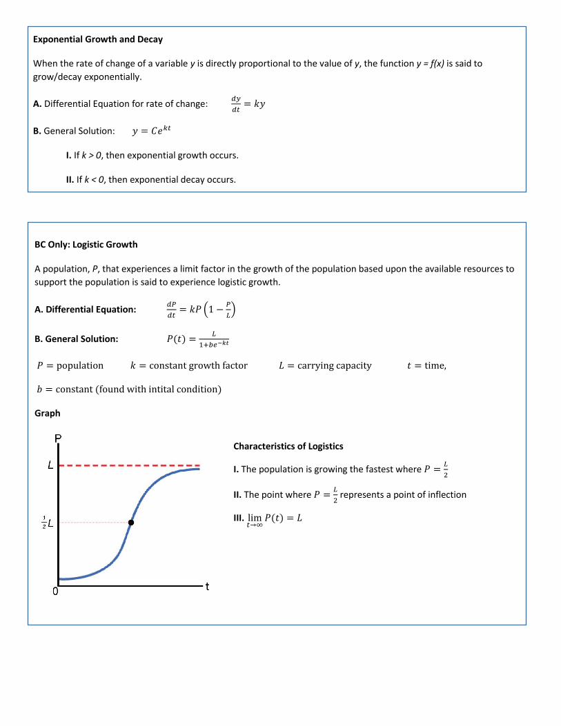
BC Only: Logistic Growth

A population, P, that experiences a limit factor in the growth of the population based upon the available resources to

support the population is said to experience logistic growth.

A. Differential Equation: 𝑑𝑃

𝑑𝑡= 𝑘𝑃 (1 −

𝑃

𝐿)

B. General Solution: 𝑃(𝑡) =𝐿

1+𝑏𝑒−𝑘𝑡

𝑃 = population 𝑘 = constant growth factor 𝐿 = carrying capacity 𝑡 = time,

𝑏 = constant (found with intital condition)

Graph

Exponential Growth and Decay

When the rate of change of a variable y is directly proportional to the value of y, the function y = f(x) is said to

grow/decay exponentially.

A. Differential Equation for rate of change: 𝑑𝑦

𝑑𝑡= 𝑘𝑦

B. General Solution: 𝑦 = 𝐶𝑒𝑘𝑡

I. If k > 0, then exponential growth occurs.

II. If k < 0, then exponential decay occurs.

Characteristics of Logistics

I. The population is growing the fastest where 𝑃 =𝐿

2

II. The point where 𝑃 =𝐿

2 represents a point of inflection

III. lim𝑡→∞

𝑃(𝑡) = 𝐿

Area Between Two Curves

A. Let 𝑦 = 𝑓(𝑥) and 𝑦 = 𝑔(𝑥)represent two functions such that 𝑓(𝑥) ≥ 𝑔(𝑥)(meaning the function f is always above

the function g on the graph) for every x on the interval [a, b].

Area Between Curves = ∫ [𝑓(𝑥) − 𝑔(𝑥)]𝑏

𝑎

𝑑𝑥

B. Let 𝑥 = 𝑓(𝑦) and 𝑥 = 𝑔(𝑦)represent two functions such that 𝑓(𝑦) ≥ 𝑔(𝑦)(meaning the function f is always to the

right of the function g on the graph) for every y on the interval [a, b].

Area Between Curves = ∫ [𝑓(𝑦) − 𝑔(𝑦)]𝑏

𝑎

𝑑𝑦

Volumes of a Solid of Revolution: Disk Method

If a defined region, bounded by a differentiable function f, on a graph is rotated about a line, the resulting solid is called

a solid of revolution and the line is called the axis of revolution. The disk method is used when the defined region

boarders the axis of revolution over the entire interval [a, b]

A. Revolving around the x – axis

Volume = 𝜋 ∫ (𝑓(𝑥))2

𝑑𝑥𝑏

𝑎

B. Revolving around the y – axis

Volume = 𝜋 ∫ (𝑓(𝑦))2

𝑑𝑦𝑏

𝑎

C. Revolving around a horizontal line y = k

Volume = 𝜋 ∫ (𝑓(𝑥) − 𝑘)2𝑑𝑥𝑏

𝑎

D. Revolving around a vertical line x = m

Volume = 𝜋 ∫ (𝑓(𝑦) − 𝑚)2𝑑𝑦𝑏

𝑎

Volumes of a Solid of Revolution: Washer Method

If a defined region, bounded by a differentiable function f, on a graph is rotated about a line, the resulting solid is called

a solid of revolution and the line is called the axis of revolution. The washer method is used when the defined region has

space between the axis of revolution on the interval [a, b]

A. Revolving around the x – axis, where 𝑓(𝑥) ≥ 𝑔(𝑥)(meaning the function f is always above the function g on the

graph) for every x on the interval [a, b].

Volume = 𝜋 ∫ ([𝑓(𝑥)]2 − [𝑔(𝑥)]2)𝑑𝑥𝑏

𝑎

B. Revolving around the y – axis, where 𝑓(𝑦) ≥ 𝑔(𝑦)(meaning the function f is always to the right of the function g on the graph)

Volume = 𝜋 ∫ ([𝑓(𝑦)]2 − [𝑔(𝑦)]2)𝑑𝑦𝑏

𝑎

C. Revolving around a horizontal line y = k, where 𝑓(𝑥) ≥ 𝑔(𝑥)(meaning the function f is always above the function g on the graph) for every x on the interval [a, b].

Volume = 𝜋 ∫ ([𝑓(𝑥) − 𝑘]2 − [𝑔(𝑥) − 𝑘]2)𝑑𝑥𝑏

𝑎

D. Revolving around a vertical line x = m, where 𝑓(𝑦) ≥ 𝑔(𝑦)(meaning the function f is always to the right of the function g on the graph)

Volume = 𝜋 ∫ ([𝑓(𝑦) − 𝑚]2 − [𝑔(𝑦) − 𝑚]2)𝑑𝑦𝑏

𝑎

Volumes of Known Cross Sections

If a defined region, bounded by a differentiable function f, is used at the base of a solid, then the volume of the solid can

be found by integrated using known area formulas.

For the cross sections perpendicular to the x – axis and a region bounded by a function f , on the interval [a, b], and the

axis.

I. Cross sections are squares

Volume = ∫ [𝑓(𝑥)]2𝑑𝑥𝑏

𝑎

II. Cross sections are equilateral triangles

Volume =√3

4∫ [𝑓(𝑥)]2𝑑𝑥

𝑏

𝑎

III. Cross sections are isosceles right triangles with a leg in the base

Volume =1

2∫ [𝑓(𝑥)]2𝑑𝑥

𝑏

𝑎

IV. Cross sections are isosceles right triangles with the hypotenuse in the base

Volume =1

4∫ [𝑓(𝑥)]2𝑑𝑥

𝑏

𝑎

V. Cross sections are semicircles (with diameter in base)

Volume =𝜋

8∫ [𝑓(𝑥)]2𝑑𝑥

𝑏

𝑎

VI. Cross sections are semicircles (with radius in base)

Volume =𝜋

2∫ [𝑓(𝑥)]2𝑑𝑥

𝑏

𝑎

Differential Equations

A differential equation is an equation involving an unknown function and one or more of its derivatives

𝑑𝑦

𝑑𝑥= 𝑓(𝑥, 𝑦) Usually expressed as a derivative equal to an expression in terms of x and/or y.

To solve differential equations, use the technique of separation of variables.

Given the differential equation 𝑑𝑦

𝑑𝑥=

𝑥𝑦

(𝑥2+1)

Step 1: Separate the variables, putting all y’s on one side, with dy in the numerator, and all x’s on the other side,

with dx in the numerator.

1

𝑦𝑑𝑦 =

𝑥

(𝑥2 + 1)𝑑𝑥

Step 2: Integrate both sides of the equation.

ln|𝑦| =1

2ln √𝑥2 + 1 + 𝐶

Step 3: Solve the equation for y.

𝑦 = 𝐶√𝑥2 + 1

Given the differential equation 𝑑𝑦

𝑑𝑥= 2𝑥2 with the initial condition 𝑦(3) = 10.

A. The general solution to a differential equation is left with the constant of integration, C, undefined.

𝑑𝑦 = 2𝑥2 𝑑𝑥 → ∫ 𝑑𝑦 = ∫ 2𝑥2 𝑑𝑥 → 𝑦 =2

3𝑥3 + 𝐶

B. The particular solution uses the given initial condition to calculate the value of C.

10 =2

3(3)3 + 𝐶 → 𝐶 = −8 → 𝑦 =

2

3𝑥3 − 8

BC Only: Euler’s Method for Approximating the Solution of a Differential Equation

Euler’s method uses a linear approximation with increments (steps), h, for approximating the solution to a given

differential equation, 𝑑𝑦

𝑑𝑥= 𝐹(𝑥, 𝑦), with a given initial value.

Process: Initial value (𝑥0, 𝑦0)

𝑥1 = 𝑥0 + ℎ 𝑦1 = 𝑦0 + ℎ ∙ 𝐹(𝑥0, 𝑦0)

𝑥2 = 𝑥1 + ℎ 𝑦2 = 𝑦1 + ℎ ∙ 𝐹(𝑥1, 𝑦1)

𝑥3 = 𝑥2 + ℎ 𝑦3 = 𝑦2 + ℎ ∙ 𝐹(𝑥2, 𝑦2)

* This process repeats until the desired y – value is given.

Slope Field

The derivative of a function gives the value of the slope of the function at each point (x, y). A slope field is a graphical

representation of all of the possible solutions to a given differential equation. The slope field is generated by plugging in

the coordinates of every point (x, y) into the differential equation and drawing a small segment of the tangent line at

each point.

Given the differential equation 𝑑𝑦

𝑑𝑥=

𝑥

𝑦

𝑑𝑦

𝑑𝑥|

(0,0)=

0

0 𝑢𝑛𝑑𝑒𝑓𝑖𝑛𝑒𝑑

𝑑𝑦

𝑑𝑥|

(0,±1)= 0

𝑑𝑦

𝑑𝑥|

(1,2)=

1

2

BC Only: Testing for Convergence/Divergence of a Series

Sequence of Partial Sums

Given the series

∑ 𝑎𝑛 = 𝑎1 + 𝑎2 + 𝑎3 + ⋯

The sequence of partial sums for the series is

𝑆1 = 𝑎1 𝑆2 = 𝑎1 + 𝑎2 𝑆3 = 𝑎1 + 𝑎2 + 𝑎3 … 𝑆𝑛 = 𝑎1 + 𝑎2 + 𝑎3 + ⋯ + 𝑎𝑛

If lim𝑛→∞

𝑆𝑛 = 𝑆, then ∑ 𝑎𝑛 converges to 𝑆.

Nth Term

If the terms of a sequence do not converge to 0, then the series must diverge.

𝐈. If lim𝑛→∞

𝑎𝑛 ≠ 0, then ∑ 𝑎𝑛 diverges.

𝐈𝐈. If lim𝑛→∞

𝑎𝑛 = 0, then the test is inconclusive.

P – Series

The form of a p – series is

∑1

𝑛𝑝

𝐈. If 𝑝 > 1, then the series converges.

𝐈𝐈. If 𝑝 < 1, then the series diverges.

*These are only

three example

points. You

would do this for

every point in

the given region

of the graph.

Geometric Series A geometric series is any series of the form

∑ 𝑎𝑟𝑛

∞

𝑛=0

𝐈. If |𝑟| < 1, then the series converges to𝑎

1−𝑟 *Series must be indexed at n = 0

𝐈𝐈. If |𝑟| > 1, then the series diverges.

Telescoping Series

A telescoping series is any series of the form

∑ 𝑎𝑛 − 𝑎𝑛+1

*Convergence and divergence is found using a sequence of partial sums

*Partial decomposition may be used to break a single rational series into the difference of two series that form the telescoping series.

Integral

If f is positive, continuous, and decreasing for 𝑥 ≥ 1, then

∑ 𝑎𝑛 and ∫ 𝑓(𝑥)𝑑𝑥∞

1

∞

𝑛=1

either both converge or both diverge.

Alternating Series

A series, containing both positive terms, negative terms, and 𝑎𝑛 > 0, of the form

∑(−1)𝑛 𝑎𝑛

∞

𝑛=1

or ∑(−1)𝑛+1 𝑎𝑛

∞

𝑛=1

The series’ converge if both of the following conditions are met

I. 𝑎𝑛+1 ≤ 𝑎𝑛 for all n

II. lim𝑛→∞

𝑎𝑛 = 0

Direct Comparison

When comparing two series, if 𝑎𝑛 ≤ 𝑏𝑛 for all n,

𝐈. If ∑ 𝑎𝑛 diverges, then ∑ 𝑏𝑛 diverges.

𝐈𝐈. If ∑ 𝑏𝑛 converges, then ∑ 𝑎𝑛 converges.

*The convergence or divergence of the series chosen for comparison should be known

Limit Comparison

If 𝑎𝑛 > 0 and 𝑏𝑛 > 0 and lim𝑛→∞

𝑎𝑛

𝑏𝑛= 𝐿 , where L is finite and positive, then the series

∑ 𝑎𝑛 and ∑ 𝑏𝑛 either both converge or both diverge. *The convergence or divergence of the series chosen for comparison should be known

*When choosing a series to compare to, disregard all but the highest powers (growth factor) in the numerator and denominator

Root

Given a series ∑ 𝑎𝑛

𝐈. If lim𝑛→∞

√|𝑎𝑛|𝑛

< 1, then ∑ 𝑎𝑛 converges.

𝐈𝐈. If lim𝑛→∞

√|𝑎𝑛|𝑛> 1, then ∑ 𝑎𝑛 diverges.

𝐈𝐈𝐈. If lim𝑛→∞

√|𝑎𝑛|𝑛

= 1, then the root test is inconclusive.

*This is a test for absolute convergence

Ratio

Given a series ∑ 𝑎𝑛

𝐈. If lim𝑛→∞

|𝑎𝑛+1

𝑎𝑛| < 1, then ∑ 𝑎𝑛 converges.

𝐈𝐈. If lim𝑛→∞

|𝑎𝑛+1

𝑎𝑛| > 1, then ∑ 𝑎𝑛 diverges.

𝐈𝐈𝐈. If lim𝑛→∞

|𝑎𝑛+1

𝑎𝑛| = 1, then the ratio test is inconclusive.

*This is a test for absolute convergence

BC Only: Absolute vs Conditional Convergence

For a series, ∑ 𝑎𝑛, with both positive and negative terms

𝐀. If ∑|𝑎𝑛|

∞

𝑛=1

converges, then ∑ 𝑎𝑛

∞

𝑛=1

also converges. ∑ 𝑎𝑛

∞

𝑛=1

is said to be absolutely convergent.

𝐁. If ∑|𝑎𝑛|

∞

𝑛=1

diverges, but ∑ 𝑎𝑛

∞

𝑛=1

converges, ∑ 𝑎𝑛

∞

𝑛=1

is said to be conditionally convergent.

BC Only: Alternating Series Remainder Theorem

Given ∑ 𝑎𝑛is a convergent alternating series, the error associated with approximating the sum of the series by the first n

terms is less than or equal to the first omitted term.

∑(−1)𝑛+1𝑎𝑛 = 𝑆 ≈ 𝑆𝑛 = 𝑎1 − 𝑎2 + ⋯ + (−1)𝑛+1𝑎𝑛

∞

𝑛=1

Error = |𝑆 − 𝑆𝑛| ≤ |𝑎𝑛+1|

BC Only: Power Series

A. Power Series Structure and Characteristics

∑ 𝑎𝑛𝑥𝑛

∞

𝑛=0

= 𝑎0 + 𝑎1𝑥 + 𝑎2𝑥2 + ⋯ + 𝑎𝑛𝑥𝑛 + ⋯ power series centered at 𝑥 = 0

∑ 𝑎𝑛(𝑥 − 𝑐)𝑛

∞

𝑛=0

= 𝑎0 + 𝑎1(𝑥 − 𝑐) + 𝑎2(𝑥 − 𝑐)2 + ⋯ + 𝑎𝑛(𝑥 − 𝑐)𝑛 + ⋯ power series centered at 𝑥 = 𝑐

A function f can be represented by a power series , where the power series converges to the function in one of

three ways:

I. The power series only converges at the center x = c.

II. The power series converges for all real values of x.

III. The power series converges for some interval of values such that |𝑥 − 𝑐| < 𝑅, where R is the radius

of convergence of the power series.

B. Interval of Convergence: Find this by applying the Ratio to the given series.

I. If 𝑅 = 0, then the series converges only at x = c.

II. If 𝑅 = ∞, then the series converges for all real values of x.

III. If the Ratio Test results in an expression of the form |𝑥 − 𝑐| < 𝑅, then the interval of convergence is

of the form 𝑐 − 𝑅 < 𝑥 < 𝑐 + 𝑅.

*The convergence at the endpoints of the interval of convergence should be tested separately.

BC Only: Taylor and Maclaurin Series (specific power series)

If a function of f has derivatives of all orders at x = c, then the series is called a Taylor Series for f centered at c. A Taylor

series centered at 0 is also known as a Maclaurin Series.

A. Maclaurin Series

𝑓(𝑥) = 𝑓(0) + 𝑓′(0)𝑥 + 𝑓′′(0)𝑥2

2!+ 𝑓′′′(0)

𝑥3

3!+ ⋯ + 𝑓(𝑛)(0)

𝑥𝑛

𝑛!+ ⋯ = ∑ 𝑓(𝑛)(0)

∞

𝑛=0

𝑥𝑛

𝑛!

B. Taylor Series

𝑓(𝑥) = 𝑓(𝑐) + 𝑓′(𝑐)(𝑥 − 𝑐) + 𝑓′′(𝑐)(𝑥 − 𝑐)2

2!+ 𝑓′′′(𝑐)

(𝑥 − 𝑐)3

3!+ ⋯ + 𝑓(𝑛)(𝑐)

(𝑥 − 𝑐)𝑛

𝑛!+ ⋯ = ∑ 𝑓(𝑛)(𝑐)

∞

𝑛=0

(𝑥 − 𝑐)𝑛

𝑛!

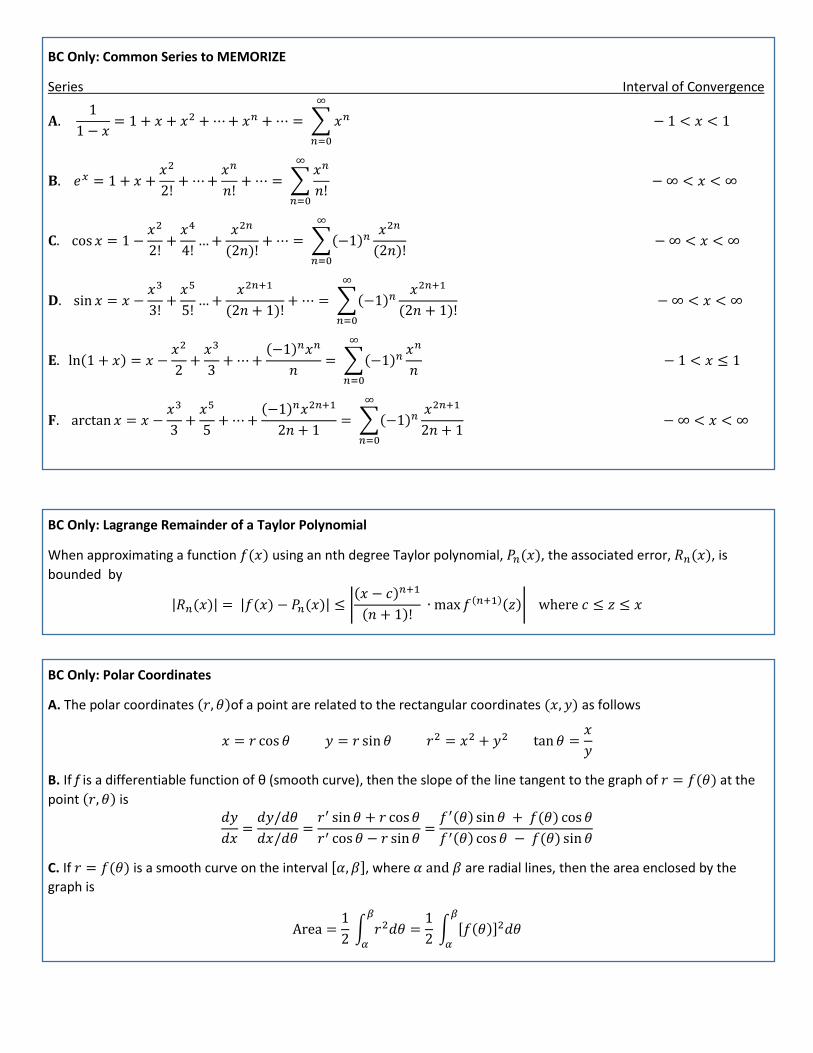
BC Only: Common Series to MEMORIZE

Series Interval of Convergence

𝐀. 1

1 − 𝑥= 1 + 𝑥 + 𝑥2 + ⋯ + 𝑥𝑛 + ⋯ = ∑ 𝑥𝑛

∞

𝑛=0

− 1 < 𝑥 < 1

𝐁. 𝑒𝑥 = 1 + 𝑥 +𝑥2

2!+ ⋯ +

𝑥𝑛

𝑛!+ ⋯ = ∑

𝑥𝑛

𝑛!

∞

𝑛=0

− ∞ < 𝑥 < ∞

𝐂. cos 𝑥 = 1 −𝑥2

2!+

𝑥4

4!… +

𝑥2𝑛

(2𝑛)!+ ⋯ = ∑(−1)𝑛

𝑥2𝑛

(2𝑛)!

∞

𝑛=0

− ∞ < 𝑥 < ∞

𝐃. sin 𝑥 = 𝑥 −𝑥3

3!+

𝑥5

5!… +

𝑥2𝑛+1

(2𝑛 + 1)!+ ⋯ = ∑(−1)𝑛

𝑥2𝑛+1

(2𝑛 + 1)!

∞

𝑛=0

− ∞ < 𝑥 < ∞

𝐄. ln(1 + 𝑥) = 𝑥 −𝑥2

2+

𝑥3

3+ ⋯ +

(−1)𝑛𝑥𝑛

𝑛= ∑(−1)𝑛

𝑥𝑛

𝑛

∞

𝑛=0

− 1 < 𝑥 ≤ 1

𝐅. arctan 𝑥 = 𝑥 −𝑥3

3+

𝑥5

5+ ⋯ +

(−1)𝑛𝑥2𝑛+1

2𝑛 + 1= ∑(−1)𝑛

𝑥2𝑛+1

2𝑛 + 1

∞

𝑛=0

− ∞ < 𝑥 < ∞

BC Only: Lagrange Remainder of a Taylor Polynomial

When approximating a function 𝑓(𝑥) using an nth degree Taylor polynomial, 𝑃𝑛(𝑥), the associated error, 𝑅𝑛(𝑥), is

bounded by

|𝑅𝑛(𝑥)| = |𝑓(𝑥) − 𝑃𝑛(𝑥)| ≤ |(𝑥 − 𝑐)𝑛+1

(𝑛 + 1)! ∙ max 𝑓(𝑛+1)(𝑧)| where 𝑐 ≤ 𝑧 ≤ 𝑥

BC Only: Polar Coordinates

A. The polar coordinates (𝑟, 𝜃)of a point are related to the rectangular coordinates (𝑥, 𝑦) as follows

𝑥 = 𝑟 cos 𝜃 𝑦 = 𝑟 sin 𝜃 𝑟2 = 𝑥2 + 𝑦2 tan 𝜃 =𝑥

𝑦

B. If f is a differentiable function of θ (smooth curve), then the slope of the line tangent to the graph of 𝑟 = 𝑓(𝜃) at the

point (𝑟, 𝜃) is 𝑑𝑦

𝑑𝑥=

𝑑𝑦/𝑑𝜃

𝑑𝑥/𝑑𝜃=

𝑟′ sin 𝜃 + 𝑟 cos 𝜃

𝑟′ cos 𝜃 − 𝑟 sin 𝜃=

𝑓′(𝜃) sin 𝜃 + 𝑓(𝜃) cos 𝜃

𝑓′(𝜃) cos 𝜃 − 𝑓(𝜃) sin 𝜃

C. If 𝑟 = 𝑓(𝜃) is a smooth curve on the interval [𝛼, 𝛽], where 𝛼 and 𝛽 are radial lines, then the area enclosed by the

graph is

Area =1

2 ∫ 𝑟2𝑑𝜃

𝛽

𝛼

=1

2 ∫ [𝑓(𝜃)]2𝑑𝜃

𝛽

𝛼