AP-42, Vol. I, CH 4.3: Waste Water Collection, Treatment And Storage
46
4.3 Waste Water Collection, Treatment And Storage 4.3.1 General Many different industries generate waste water streams that contain organic compounds. Nearly all of these streams undergo collection, contaminant treatment, and/or storage operations before they are finally discharged into either a receiving body of water or a municipal treatment plant for further treatment. During some of these operations, the waste water is open to the atmosphere, and volatile organic compounds (VOC) may be emitted from the waste water into the air. Industrial waste water operations can range from pretreatment to full-scale treatment processes. In a typical pretreatment facility, process and/or sanitary waste water and/or storm water runoff is collected, equalized, and/or neutralized and then discharged to a municipal waste water plant, also known as a publicly owned treatment works (POTWs), where it is then typically treated further by biodegradation. In a full-scale treatment operation, the waste water must meet Federal and/or state quality standards before it is finally discharged into a receiving body of water. Figure 4.3-1 shows a generic example of collection, equalization, neutralization, and biotreatment of process waste water in a full- scale industrial treatment facility. If required, chlorine is added as a disinfectant. A storage basin contains the treated water until the winter months (usually January to May), when the facility is allowed to discharge to the receiving body of water. In the illustration, the receiving body of water is a slow-flowing stream. The facility is allowed to discharge in the rainy season when the facility waste water is diluted. Figure 4.3-1 also presents a typical treatment system at a POTW waste water facility. Industrial waste water sent to POTWs may be treated or untreated. POTWs may also treat waste water from residential, institutional, and commercial facilities; from infiltration (water that enters the sewer system from the ground); and/or storm water runoff. These types of waste water generally do not contain VOCs. A POTW usually consists of a collection system, primary settling, biotreatment, secondary settling, and disinfection. Collection, treatment, and storage systems are facility-specific. All facilities have some type of collection system, but the complexity will depend on the number and volume of waste water streams generated. As mentioned above, treatment and/or storage operations also vary in size and degree of treatment. The size and degree of treatment of waste water streams will depend on the volume and degree of contamination of the waste water and on the extent of contaminant removal desired. 4.3.1.1 Collection Systems - There are many types of waste water collection systems. In general, a collection system is located at or near the point of waste water generation and is designed to receive 1 or more waste water streams and then to direct these streams to treatment and/or storage systems. A typical industrial collection system may include drains, manholes, trenches, junction boxes, sumps, lift stations, and/or weirs. Waste water streams from different points throughout the industrial facility normally enter the collection system through individual drains or trenches connected to a main sewer line. The drains and trenches are usually open to the atmosphere. Junction boxes, sumps, 9/91 (Reformatted 1/95) Evaporation Loss Sources 4.3-1
Transcript of AP-42, Vol. I, CH 4.3: Waste Water Collection, Treatment And Storage

4.3 Waste Water Collection, Treatment And Storage
4.3.1 General
Many different industries generate waste water streams that contain organic compounds.Nearly all of these streams undergo collection, contaminant treatment, and/or storage operations beforethey are finally discharged into either a receiving body of water or a municipal treatment plant forfurther treatment. During some of these operations, the waste water is open to the atmosphere, andvolatile organic compounds (VOC) may be emitted from the waste water into the air.
Industrial waste water operations can range from pretreatment to full-scale treatment processes.In a typical pretreatment facility, process and/or sanitary waste water and/or storm water runoff iscollected, equalized, and/or neutralized and then discharged to a municipal waste water plant, alsoknown as apublicly owned treatment works (POTWs), where it is then typically treated further bybiodegradation.
In a full-scale treatment operation, the waste water must meet Federal and/or state qualitystandards before it is finally discharged into a receiving body of water. Figure 4.3-1 shows agenericexample of collection, equalization, neutralization, and biotreatment of process waste water in a full-scale industrial treatment facility. If required, chlorine is added as adisinfectant. A storage basincontains the treated water until the winter months (usually January to May), when the facility isallowed to discharge to the receiving body of water. In the illustration, the receiving body of water isa slow-flowing stream. The facility is allowed to discharge in the rainy season when the facility wastewater is diluted.
Figure 4.3-1 also presents atypical treatment system at a POTW waste water facility.Industrial waste water sent to POTWs may be treated or untreated. POTWs may also treat wastewater from residential, institutional, and commercial facilities; from infiltration (water that enters thesewer system from the ground); and/or storm water runoff. These types of waste water generally donot contain VOCs. A POTW usually consists of a collection system, primary settling, biotreatment,secondary settling, and disinfection.
Collection, treatment, and storage systems are facility-specific. Al l facilities have some type ofcollection system, but the complexity wil l depend on the number and volume of waste water streamsgenerated. As mentioned above, treatment and/or storage operations also vary in size and degree oftreatment. The size and degree of treatment of waste water streams wil l depend on the volume anddegree of contamination of the waste water and on the extent of contaminant removal desired.
4.3.1.1 Collection Systems -There are many types of waste water collection systems. In general, a collection system is
located at or near the point of waste water generation and is designed to receive 1 or more waste waterstreams and then to direct these streams to treatment and/or storage systems.
A typical industrial collection system may include drains, manholes, trenches, junction boxes,sumps, lif t stations, and/or weirs. Waste water streams from different points throughout the industrialfacility normally enter the collection system through individual drains or trenches connected to a mainsewer line. The drains and trenches are usually open to the atmosphere. Junction boxes, sumps,
9/91 (Reformatted 1/95) Evaporation Loss Sources 4.3-1

Figure 4.3.1. Typical waste water collection and treatment systems for industrial and municipal facilities.
4.3-2E
MIS
SIO
NF
AC
TO
RS
(Reform
atted1/95)9/91

trenches, lift stations, and weirs will be located at points requiring waste water transport from 1 area ortreatment process to another.
A typical POTW facility collection system will contain a lift station, trenches, junction boxes,and manholes. Waste water is received into the POTW collection system through open sewer linesfrom all sources of influent waste water. As mentioned previously, these sources may convey sanitary,pretreated or untreated industrial, and/or storm water runoff waste water.
The following paragraphs briefly describe some of the most common types of waste watercollection system components found in industrial and POTW facilities. Because the arrangement ofcollection system components is facility-specific, the order in which the collection system descriptionsare presented is somewhat arbitrary.
Waste water streams normally are introduced into the collection system through individual orarea drains, which can be open to the atmosphere or sealed to prevent waste water contact with theatmosphere. In industry, individual drains may be dedicated to a single source or piece of equipment.Area drains will serve several sources and are located centrally among the sources or pieces ofequipment that they serve.
Manholes into sewer lines permit service, inspection, and cleaning of a line. They may belocated where sewer lines intersect or where there is a significant change in direction, grade, or sewerline diameter.
Trenches can be used to transport industrial waste water from point of generation to collectionunits such as junction boxes and lift station, from 1 process area of an industrial facility to another, orfrom 1 treatment unit to another. POTWs also use trenches to transport waste water from 1 treatmentunit to another. Trenches are likely to be either open or covered with a safety grating.
Junction boxes typically serve several process sewer lines, which meet at the junction box tocombine multiple waste water streams into 1. Junction boxes normally are sized to suit the total flowrate of the entering streams.
Sumps are used typically for collection and equalization of waste water flow from trenches orsewer lines before treatment or storage. They are usually quiescent and open to the atmosphere.
Lift stations are usually the last collection unit before the treatment system, accepting wastewater from 1 or several sewer lines. Their main function is to lift the collected waste water to atreatment and/or storage system, usually by pumping or by use of a hydraulic lift, such as a screw.
Weirs can act as open channel dams, or they can be used to discharge cleaner effluent from asettling basin, such as a clarifier. When used as a dam, the weir’s face is normally alignedperpendicular to the bed and walls of the channel. Water from the channel usually flows over the weirand falls to the receiving body of water. In some cases, the water may pass through a notch oropening in the weir face. With this type of weir, flow rate through the channel can be measured.Weir height, generally the distance the water falls, is usually no more than 2 meters (6 feet). Atypical clarifier weir is designed to allow settled waste water to overflow to the next treatment process.The weir is generally placed around the perimeter of the settling basin, but it can also be towards themiddle. Clarifier weir height is usually only about 0.1 meters (4 inches).
9/91 (Reformatted 1/95) Evaporation Loss Sources 4.3-3

4.3.1.2 Treatment And/Or Storage Systems -These systems are designed to hold liquid wastes or waste water for treatment, storage, or
disposal. They are usually composed of various types of earthen and/or concrete-lined basins, knownas surface impoundments. Storage systems are used typically for accumulating waste water before itsultimate disposal, or for temporarily holding batch (intermittent) streams before treatment.
Treatment systems are divided into 3 categories: primary, secondary, or tertiary, depending ontheir design, operation, and application. In primary treatment systems, physical operations removefloatable and settleable solids. In secondary treatment systems, biological and chemical processesremove most of the organic matter in the waste water. In tertiary treatment systems, additionalprocesses remove constituents not taken out by secondary treatment.
Examples of primary treatment include oil/water separators, primary clarification, equalizationbasins, and primary treatment tanks. The first process in an industrial waste water treatment plant isoften the removal of heavier solids and lighter oils by means of oil/water separators. Oils are usuallyremoved continuously with a skimming device, while solids can be removed with a sludge removalsystem.
In primary treatment, clarifiers are usually located near the beginning of the treatment processand are used to settle and remove settleable or suspended solids contained in the influent waste water.Figure 4.3-2 presents an example design of a clarifier. Clarifiers are generally cylindrical and aresized according to both the settling rate of the suspended solids and the thickening characteristics ofthe sludge. Floating scum is generally skimmed continuously from the top of the clarifier, whilesludge is typically removed continuously from the bottom of the clarifier.
Equalization basins are used to reduce fluctuations in the waste water flow rate and organiccontent before the waste is sent to downstream treatment processes. Flow rate equalization results in amore uniform effluent quality in downstream settling units such as clarifiers. Biological treatmentperformance can also benefit from the damping of concentration and flow fluctuations, protectingbiological processes from upset or failure from shock loadings of toxic or treatment-inhibitingcompounds.
In primary treatment, tanks are generally used to alter the chemical or physical properties ofthe waste water by, for example, neutralization and the addition and dispersion of chemical nutrients.Neutralization can control the pH of the waste water by adding an acid or a base. It usually precedesbiotreatment, so that the system is not upset by high or low pH values. Similarly, chemical nutrientaddition/dispersion precedes biotreatment, to ensure that the biological organisms have sufficientnutrients.
An example of a secondary treatment process is biodegradation. Biological waste treatmentusually is accomplished by aeration in basins with mechanical surface aerators or with a diffused airsystem. Mechanical surface aerators float on the water surface and rapidly mix the water. Aeration ofthe water is accomplished through splashing. Diffused air systems, on the other hand, aerate the waterby bubbling oxygen through the water from the bottom of the tank or device. Figure 4.3-3 presents anexample design of a mechanically aerated biological treatment basin. This type of basin is usually anearthen or concrete-lined pond and is used to treat large flow rates of waste water. Waste waters withhigh pollutant concentrations, and in particular high-flow sanitary waste waters, aretypically treated using an activated sludge system where biotreatment is followed by secondaryclarification. In this system, settled solids containing biomass are recycled from clarifier sludge to thebiotreatment system. This creates a high biomass concentration and therefore allows biodegradation tooccur over a shorter residence time. An example of a tertiary treatment process is nutrient
4.3-4 EMISSION FACTORS (Reformatted 1/95)9/91

Figure 4.3-2. Example clarifier configuration.
Figure 4.3-3. Example aerated biological treatment basin.
9/91 (Reformatted 1/95) Evaporation Loss Sources 4.3-5
removal. Nitrogen and phosphorus are removed after biodegradation as a final treatment step beforewaste water is discharged to a receiving body of water.
4.3.1.3 Applications -As previously mentioned, waste water collection, treatment, and storage are common in many
industrial categories and in POTW. Most industrial facilities and POTW collect, contain, and treatwaste water. However, some industries do not treat their waste water, but use storage systems fortemporary waste water storage or for accumulation of waste water for ultimate disposal. For example,the Agricultural Industry does little waste water treatment but needs waste water storage systems,while the Oil and Gas Industry also has a need for waste water disposal systems.
The following are waste water treatment and storage applications identified by type ofindustry:
1. Mining And Milling Operations - Storage of various waste waters such as acid minewater, solvent wastes from solution mining, and leachate from disposed mining wastes.Treatment operations include settling, separation, washing, sorting of mineral productsfrom tailings, and recovery of valuable minerals by precipitation.
2. Oil And Gas Industry - One of the largest sources of waste water. Operations treatbrine produced during oil extraction and deep-well pressurizing operations, oil-watermixtures, gaseous fluids to be separated or stored during emergency conditions, anddrill cuttings and drilling muds.
3. Textile And Leather Industry - Treatment and sludge disposal. Organic species treatedor disposed of include dye carriers such as halogenated hydrocarbons and phenols.Heavy metals treated or disposed of include chromium, zinc, and copper. Tanning andfinishing wastes may contain sulfides and nitrogenous compounds.
4. Chemical And Allied Products Industry - Process waste water treatment and storage,and sludge disposal. Waste constituents are process-specific and include organics andorganic phosphates, fluoride, nitrogen compounds, and assorted trace metals.
5. Other Industries - Treatment and storage operations are found at petroleum refining,primary metals production, wood treating, and metal finishing facilities. Variousindustries store and/or treat air pollution scrubber sludge and dredging spoils sludge (i.e., settled solids removed from the floor of a surface impoundment).
4.3.2 Emissions
VOCs are emitted from waste water collection, treatment, and storage systems throughvolatilization of organic compounds at the liquid surface. Emissions can occur by diffusive orconvective mechanisms, or both. Diffusion occurs when organic concentrations at the water surfaceare much higher than ambient concentrations. The organics volatilize, or diffuse into the air, in anattempt to reach equilibrium between aqueous and vapor phases. Convection occurs when air flowsover the water surface, sweeping organic vapors from the water surface into the air. The rate ofvolatilization relates directly to the speed of the air flow over the water surface.
Other factors that can affect the rate of volatilization include waste water surface area,temperature, and turbulence; waste water retention time in the system(s); the depth of the waste waterin the system(s); the concentration of organic compounds in the waste water and their physical
4.3-6 EMISSION FACTORS (Reformatted 1/95)9/91
properties, such as volatility and diffusivity in water; the presence of a mechanism that inhibitsvolatilization, such as an oil film; or a competing mechanism, such as biodegradation.
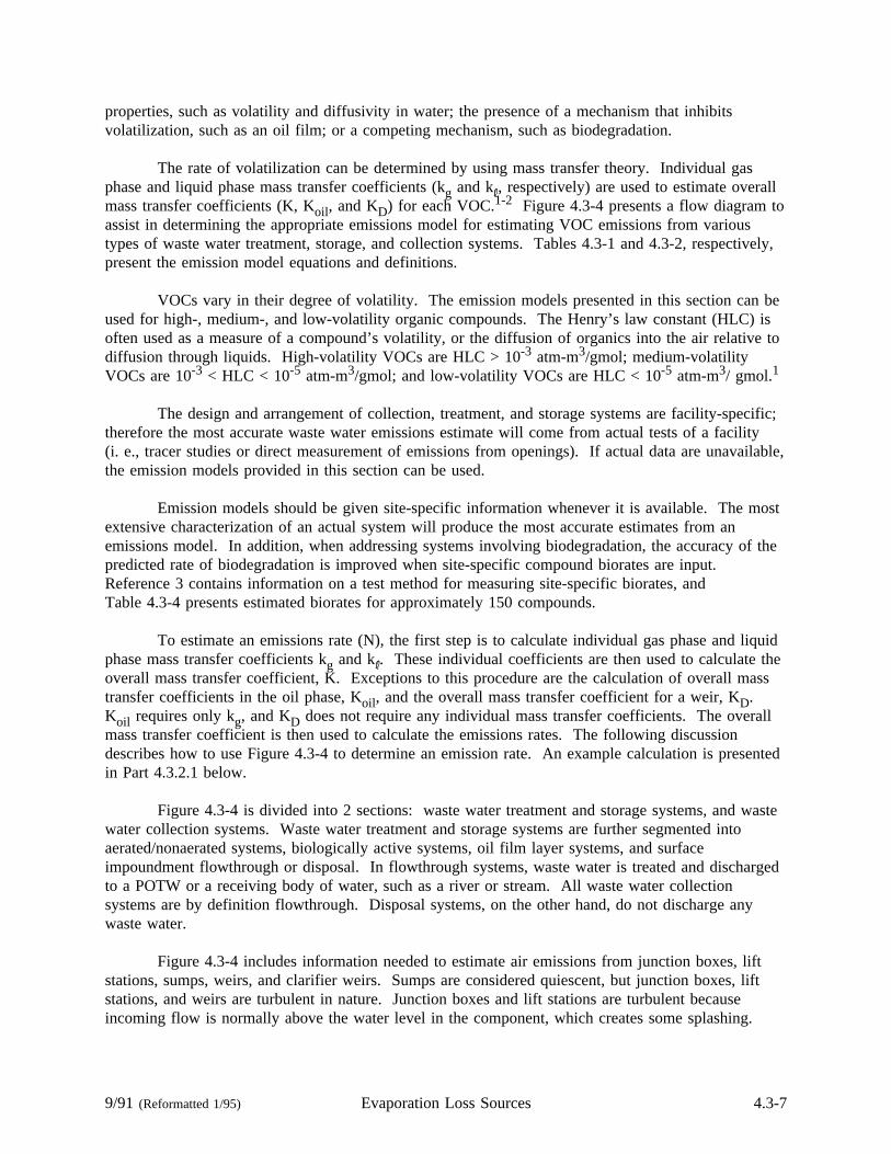
The rate of volatilization can be determined by using mass transfer theory. Individual gasphase and liquid phase mass transfer coefficients (kg and k , respectively) are used to estimate overallmass transfer coefficients (K, Koil, and KD) for each VOC.1-2 Figure 4.3-4 presents a flow diagram toassist in determining the appropriate emissions model for estimating VOC emissions from varioustypes of waste water treatment, storage, and collection systems. Tables 4.3-1 and 4.3-2, respectively,present the emission model equations and definitions.
VOCs vary in their degree of volatility. The emission models presented in this section can beused for high-, medium-, and low-volatility organic compounds. The Henry’s law constant (HLC) isoften used as a measure of a compound’s volatility, or the diffusion of organics into the air relative todiffusion through liquids. High-volatility VOCs are HLC > 10-3 atm-m3/gmol; medium-volatilityVOCs are 10-3 < HLC < 10-5 atm-m3/gmol; and low-volatility VOCs are HLC < 10-5 atm-m3/ gmol.1
The design and arrangement of collection, treatment, and storage systems are facility-specific;therefore the most accurate waste water emissions estimate will come from actual tests of a facility(i. e., tracer studies or direct measurement of emissions from openings). If actual data are unavailable,the emission models provided in this section can be used.
Emission models should be given site-specific information whenever it is available. The mostextensive characterization of an actual system will produce the most accurate estimates from anemissions model. In addition, when addressing systems involving biodegradation, the accuracy of thepredicted rate of biodegradation is improved when site-specific compound biorates are input.Reference 3 contains information on a test method for measuring site-specific biorates, andTable 4.3-4 presents estimated biorates for approximately 150 compounds.
To estimate an emissions rate (N), the first step is to calculate individual gas phase and liquidphase mass transfer coefficients kg and k . These individual coefficients are then used to calculate theoverall mass transfer coefficient, K. Exceptions to this procedure are the calculation of overall masstransfer coefficients in the oil phase, Koil, and the overall mass transfer coefficient for a weir, KD.Koil requires only kg, and KD does not require any individual mass transfer coefficients. The overallmass transfer coefficient is then used to calculate the emissions rates. The following discussiondescribes how to use Figure 4.3-4 to determine an emission rate. An example calculation is presentedin Part 4.3.2.1 below.
Figure 4.3-4 is divided into 2 sections: waste water treatment and storage systems, and wastewater collection systems. Waste water treatment and storage systems are further segmented intoaerated/nonaerated systems, biologically active systems, oil film layer systems, and surfaceimpoundment flowthrough or disposal. In flowthrough systems, waste water is treated and dischargedto a POTW or a receiving body of water, such as a river or stream. All waste water collectionsystems are by definition flowthrough. Disposal systems, on the other hand, do not discharge anywaste water.
Figure 4.3-4 includes information needed to estimate air emissions from junction boxes, liftstations, sumps, weirs, and clarifier weirs. Sumps are considered quiescent, but junction boxes, liftstations, and weirs are turbulent in nature. Junction boxes and lift stations are turbulent becauseincoming flow is normally above the water level in the component, which creates some splashing.
9/91 (Reformatted 1/95) Evaporation Loss Sources 4.3-7

Figure 4.3.4. Flow diagram for estimating VOC emissions from waste water collection,treatment, and storage systems.
4.3-8 EMISSION FACTORS (Reformatted 1/95)9/91

Table 4.3-1. MASS TRANSFER CORRELATIONS AND EMISSIONS EQUATIONSa
EquationNo. Equation
Individual liquid (k ) and gas (kg) phase mass transfer coefficients
1 k (m/s) = (2.78 x 10⁻⁶)(Dw/Dether)2/3
For: 0 < U10 < 3.25 m/s and all F/D ratios
k (m/s) = [(2.605 x 10⁻⁹)(F/D) + (1.277 x 10⁻⁷)](U10)2(Dw/Dether)
2/3
For: U10 > 3.25 m/s and 14 < F/D < 51.2
k (m/s) = (2.61 x 10⁻⁷)(U10)2(Dw/Dether)
2/3
For: U10 > 3.25 m/s and F/D > 51.2
k (m/s) = 1.0 x 10⁻⁶ + 144 x 10-4 (U*)2.2 (ScL)-0.5; U* < 0.3k (m/s) = 1.0 x 10⁻⁶ + 34.1 x 10⁻⁴ U* (ScL)-0.5; U* > 0.3
For: U10 > 3.25 m/s and F/D < 14where:
U* (m/s) = (0.01)(U10)(6.1 + 0.63(U10))0.5
ScL = µL/(ρLDw)F/D = 2 (A/π)0.5
2 kg (m/s) = (4.82 x 10⁻³)(U10)0.78 (ScG)-0.67 (de)
-0.11
where:ScG = µa/(ρaDa)
de(m) = 2(Α/π)0.5
3 k (m/s) = [(8.22 x 10⁻⁹)(J)(POWR)(1.024)(T-20)(Ot)(106) *(MWL)/(VavρL)](Dw/DO2,w)0.5
where:POWR (hp) = (total power to aerators)(V)
Vav(ft2) = (fraction of area agitated)(A)
4 kg (m/s) = (1.35 x 10⁻⁷)(Re)1.42 (P)0.4 (ScG)0.5 (Fr)-0.21(Da MWa/d)where:
Re = d2 w ρa/µaP = [(0.85)(POWR)(550 ft-lbf/s-hp)/NI] gc/(ρL(d*)5w3)
ScG = µa/(ρaDa)Fr = (d*)w2/gc
5 k (m/s) = (fair, )(Q)/[3600 s/min (hc)(πdc)]where:
fair, = 1 - 1/rr = exp [0.77(hc)
0.623(Q/πdc)0.66(Dw/DO2,w)0.66]
6 kg (m/s) = 0.001 + (0.0462(U**)(ScG)-0.67)where:
U** (m/s) = [6.1 + (0.63)(U10)]0.5(U10/100)
ScG = µa/(ρaDa)
9/91 (Reformatted 1/95) Evaporation Loss Sources 4.3-9
Table 4.3-1 (cont.).
EquationNo. Equation
Overall mass transfer coefficients for water (K) and oil (Koil) phases and for weirs (KD)
7 K = (k Keq kg)/(Keq kg + k )where:
Keq = H/(RT)
8 K (m/s) = [[MWL/(k ρL*(100 cm/m)] + [MWa/(kgρaH*55,555(100 cm/m))]]-1 MWL/[(100 cm/m)ρL]
9 Koil = kgKeqoilwhere:
Keqoil = P*ρaMWoil/(ρoil MWa Po)
10 KD = 0.16h (Dw/DO2,w)0.75
Air emissions (N)
11 N(g/s) = (1 - Ct/Co) V Co/twhere:
Ct/Co = exp[-K A t/V]
12 N(g/s) = K CL Awhere:
CL(g/m3) = Q Co/(KA + Q)
13 N(g/s) = (1 - Ct/Co) V Co/twhere:
Ct/Co = exp[-(KA + KeqQa)t/V]
14 N(g/s) = (KA + QaKeq)CLwhere:
CL(g/m3) = QCo/(KA + Q + QaKeq)
15 N(g/s) = (1 - Ct/Co) KA/(KA + Kmax bi V/Ks) V Co/twhere:
Ct/Co = exp[-Kmax bi t/Ks - K A t/V]
16 N(g/s) = K CL Awhere:
CL(g/m3) = [-b + (b2 - 4ac)0.5]/(2a)and:
a = KA/Q + 1b = Ks(KA/Q + 1) + Kmax bi V/Q - Coc = -KsCo
4.3-10 EMISSION FACTORS (Reformatted 1/95)9/91

Table 4.3-1 (cont.).
EquationNo. Equation
17 N(g/s) = (1 - Ctoil/Cooil)VoilCooil/twhere:
Ctoil/Cooil = exp[-Koil t/Doil]and:
Cooil = Kow Co/[1 - FO + FO(Kow)]Voil = (FO)(V)Doil = (FO)(V)/A
18 N(g/s) = KoilCL,oilAwhere:
CL,oil(g/m3) = QoilCooil/(KoilA + Qoil)and:
Cooil = Kow Co/[1 - FO + FO(Kow)]Qoil = (FO)(Q)
19 N(g/s) = (1 - Ct/Co)(KA + QaKeq)/(KA + QaKeq + Kmax bi V/Ks) V Co/twhere:
Ct/Co = exp[-(KA + KeqQa)t/V - Kmax bi t/Ks]
20 N(g/s) = (KA + QaKeq)CLwhere:
CL(g/m3) = [-b +(b2 - 4ac)0.5]/(2a)and:
a = (KA + QaKeq)/Q + 1b = Ks[(KA + QaKeq)/Q + 1] + Kmax bi V/Q - Coc = -KsCo
21 N (g/s) = (1 - exp[-KD])Q Co
22 N(g/s) = KoilCL,oilAwhere:
CL,oil(g/m3) = Qoil(Cooil*)/(K oilA + Qoil)and:
Cooil* = Co/FOQoil = (FO)(Q)
23 N(g/s) = (1 - Ctoil/Cooil*)(V oil)(Cooil*)/twhere:
Ctoil/Cooil* = exp[-Koil t/Doil]and:
Cooil* = Co/FOVoil = (FO)(V)Doil = (FO)(V)/A
24 N (g/s) = (1 - exp[-Kπ dc hc/Q])Q Coa All parameters in numbered equations are defined in Table 4.3-2.
9/91 (Reformatted 1/95) Evaporation Loss Sources 4.3-11
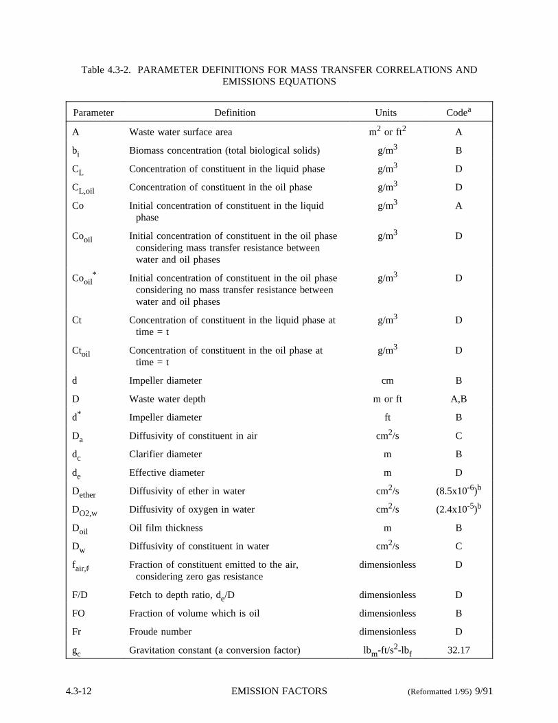
Table 4.3-2. PARAMETER DEFINITIONS FOR MASS TRANSFER CORRELATIONS ANDEMISSIONS EQUATIONS
Parameter Definition Units Codea
A Waste water surface area m2 or ft2 A
bi Biomass concentration (total biological solids) g/m3 B
CL Concentration of constituent in the liquid phase g/m3 D
CL,oil Concentration of constituent in the oil phase g/m3 D
Co Initial concentration of constituent in the liquidphase
g/m3 A
Cooil Initial concentration of constituent in the oil phaseconsidering mass transfer resistance betweenwater and oil phases
g/m3 D
Cooil* Initial concentration of constituent in the oil phase
considering no mass transfer resistance betweenwater and oil phases
g/m3 D
Ct Concentration of constituent in the liquid phase attime = t
g/m3 D
Ctoil Concentration of constituent in the oil phase attime = t
g/m3 D
d Impeller diameter cm B
D Waste water depth m or ft A,B
d* Impeller diameter ft B
Da Diffusivity of constituent in air cm2/s C
dc Clarifier diameter m B
de Effective diameter m D
Dether Diffusivity of ether in water cm2/s (8.5x10⁻⁶)b
DO2,w Diffusivity of oxygen in water cm2/s (2.4x10⁻⁵)b
Doil Oil film thickness m B
Dw Diffusivity of constituent in water cm2/s C
fair, Fraction of constituent emitted to the air,considering zero gas resistance
dimensionless D
F/D Fetch to depth ratio, de/D dimensionless D
FO Fraction of volume which is oil dimensionless B
Fr Froude number dimensionless D
gc Gravitation constant (a conversion factor) lbm-ft/s2-lbf 32.17
4.3-12 EMISSION FACTORS (Reformatted 1/95)9/91

Table 4.3-2 (cont.).
Parameter Definition Units Codea
h Weir height (distance from the waste wateroverflow to the receiving body of water)
ft B
hc Clarifier weir height m B
H Henry’s law constant of constituent atm-m3/gmol C
J Oxygen transfer rating of surface aerator lb 02/(hr-hp) B
K Overall mass transfer coefficient for transfer ofconstituent from liquid phase to gas phase
m/s D
KD Volatilization-reaeration theory mass transfercoefficient
dimensionless D
Keq Equilibrium constant or partition coefficient(concentration in gas phase/concentration inliquid phase)
dimensionless D
Keqoil Equilibrium constant or partition coefficient(concentration in gas phase/concentration in oilphase)
dimensionless D
kg Gas phase mass transfer coefficient m/s D
k Liquid phase mass transfer coefficient m/s D
Kmax Maximum biorate constant g/s-g biomass A,C
Koil Overall mass transfer coefficient for transfer ofconstituent from oil phase to gas phase
m/s D
Kow Octanol-water partition coefficient dimensionless C
Ks Half saturation biorate constant g/m3 A,C
MWa Molecular weight of air g/gmol 29
MWoil Molecular weight of oil g/gmol B
MWL Molecular weight of water g/gmol 18
N Emissions g/s D
NI Number of aerators dimensionless A,B
Ot Oxygen transfer correction factor dimensionless B
P Power number dimensionless D
P* Vapor pressure of the constituent atm C
Po Total pressure atm A
POWR Total power to aerators hp B
Q Volumetric flow rate m3/s A
9/91 (Reformatted 1/95) Evaporation Loss Sources 4.3-13
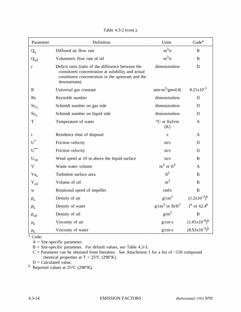
Table 4.3-2 (cont.).
Parameter Definition Units Codea
Qa Diffused air flow rate m3/s B
Qoil Volumetric flow rate of oil m3/s B
r Deficit ratio (ratio of the difference between theconstituent concentration at solubility and actualconstituent concentration in the upstream and thedownstream)
dimensionless D
R Universal gas constant atm-m3/gmol-K 8.21x10⁻⁵
Re Reynolds number dimensionless D
ScG Schmidt number on gas side dimensionless D
ScL Schmidt number on liquid side dimensionless D
T Temperature of water °C or Kelvin(K)
A
t Residence time of disposal s A
U* Friction velocity m/s D
U** Friction velocity m/s D
U10 Wind speed at 10 m above the liquid surface m/s B
V Waste water volume m3 or ft3 A
Vav Turbulent surface area ft2 B
Voil Volume of oil m3 B
w Rotational speed of impeller rad/s B
ρa Density of air g/cm3 (1.2x10⁻³)b
ρL Density of water g/cm3 or lb/ft3 1b or 62.4b
ρoil Density of oil g/m3 B
µa Viscosity of air g/cm-s (1.81x10⁻⁴)b
µL Viscosity of water g/cm-s (8.93x10⁻³)b
a Code:A = Site-specific parameter.B = Site-specific parameter. For default values, see Table 4.3-3.C = Parameter can be obtained from literature. See Attachment 1 for a list of ~150 compound
chemical properties at T = 25°C (298°K).D = Calculated value.
b Reported values at 25°C (298°K).
4.3-14 EMISSION FACTORS (Reformatted 1/95)9/91

Table 4.3-3. SITE-SPECIFIC DEFAULT PARAMETERSa
Default Parameterb Definition Default Value
General
T Temperature of water 298°K
U10 Windspeed 4.47 m/s
Biotreatment Systems
bi Biomass concentration (for biologically activesystems)
Quiescent treatment systems 50 g/m3
Aerated treatment systems 300 g/m3
Activated sludge units 4000 g/m3
POWR Total power to aerators(for aerated treatment systems)(for activated sludge)
0.75 hp/1000 ft3 (V)2 hp/1000 ft3 (V)
W Rotational speed of impeller(for aerated treatment systems) 126 rad/s (1200 rpm)
d(d*) Impeller diameter(for aerated treatment systems) 61 cm (2 ft)
Vav Turbulent surface area(for aerated treatment systems)(for activated sludge)
0.24 (A)0.52 (A)
J Oxygen transfer rating to surface aerator(for aerated treatment systems) 3 lb O2/hp hr
Ot Oxygen transfer correction factor(for aerated treatment systems) 0.83
NI Number of aerators POWR/75
Diffused Air Systems
Qa Diffused air volumetric flow rate 0.0004(V) m3/s
Oil Film Layers
MWoil Molecular weight of oil 282 g/gmol
Doil Depth of oil layer 0.001 (V/A) m
Voil Volume of oil 0.001 (V) m3
Qoil Volumetric flow rate of oil 0.001 (Q) m3/s
ρoil Density of oil 0.92 g/cm3
9/91 (Reformatted 1/95) Evaporation Loss Sources 4.3-15

Table 4.3-3 (cont.).
Default Parameterb Definition Default Value
FO Fraction of volume which is oilc 0.001
Junction Boxes
D Depth of Junction Box 0.9 m
NI Number of aerators 1
Lift Station
D Depth of Lift Station 1.5 m
NI Number of aerators 1
Sump
D Depth of sump 5.9 m
Weirs
dc Clarifier weir diameterd 28.5 m
h Weir height 1.8 m
hc Clarifier weir heighte 0.1 ma Reference 1.b As defined in Table 4.3-2.c Reference 4.d Reference 2.e Reference 5.
Waste water falls or overflows from weirs and creates splashing in the receiving body of water (bothweir and clarifier weir models). Waste water from weirs can be aerated by directing it to fall oversteps, usually only the weir model.
Assessing VOC emissions from drains, manholes, and trenches is also important indetermining the total waste water facility emissions. As these sources can be open to the atmosphereand closest to the point of waste water generation (i. e., where water temperatures and pollutantconcentrations are greatest), emissions can be significant. Currently, there are no well-establishedemission models for these collection system types. However, work is being performed to address thisneed.
Preliminary models of VOC emissions from waste collection system units have beendeveloped.4 The emission equations presented in Reference 4 are used with standard collection systemparameters to estimate the fraction of the constituents released as the waste water flows through eachunit. The fractions released from several units are estimated for high-, medium-, and low-volatilitycompounds. The units used in the estimated fractions included open drains, manhole covers, opentrench drains, and covered sumps.
4.3-16 EMISSION FACTORS (Reformatted 1/95)9/91
The numbers in Figure 4.3-4 under the columns for k , kg, Koil, KD, K, and N refer to theappropriate equations in Table 4.3-1.a Definitions for all parameters in these equations are given inTable 4.3-2. Table 4.3-2 also supplies the units that must be used for each parameter, with codes tohelp locate input values. If the parameter is coded with the letter A, a site-specific value is required.Code B also requires a site-specific parameter, but defaults are available. These defaults are typical oraverage values and are presented by specific system in Table 4.3-3.
Code C means the parameter can be obtained from literature data. Table 4.3-4 contains a listof approximately 150 chemicals and their physical properties needed to calculate emissions from wastewater, using the correlations presented in Table 4.3-1. All properties are at 25°C (77°F).A more extensive chemical properties data base is contained in Appendix C of Reference 1.)Parameters coded D are calculated values.
Calculating air emissions from waste water collection, treatment, and storage systems is acomplex procedure, especially if several systems are present. Performing the calculations by hand mayresult in errors and will be time consuming. A personal computer program called the SurfaceImpoundment Modeling System (SIMS) is now available for estimating air emissions. The program ismenu driven and can estimate air emissions from all surface impoundment models presented inFigure 4.3-4, individually or in series. The program requires for each collection, treatment, or storagesystem component, at a minimum, the waste water flow rate and component surface area. All otherinputs are provided as default values. Any available site-specific information should be entered inplace of these defaults, as the most fully characterized system will provide the most accurate emissionsestimate.
The SIMS program with user’s manual and background technical document can be obtainedthrough state air pollution control agencies and through the U. S. Environmental Protection Agency’sControl Technology Center in Research Triangle Park, NC, telephone (919) 541-0800. The user’smanual and background technical document should be followed to produce meaningful results.
The SIMS program and user’s manual also can be downloaded from EPA’s Clearinghouse ForInventories and Emission Factors (CHIEF) electronic bulletin board (BB). The CHIEF BB is open toall persons involved in air emission inventories. To access this BB, one needs a computer, modem, andcommunication package capable of communicating at up to 14,400 baud, 8 data bits, 1 stop bit, and noparity (8-N-1). This BB is part of EPA’s OAQPS Technology Transfer Network system and itstelephone number is (919) 541-5742. First-time users must register before access is allowed.
Emissions estimates from SIMS are based on mass transfer models developed by EmissionsStandards Division (ESD) during evaluations of TSDFs and VOC emissions from industrial wastewater. As a part of the TSDF project, a Lotus® spreadsheet program called CHEMDAT7 wasdeveloped for estimating VOC emissions from waste water land treatment systems, open landfills,closed landfills, and waste storage piles, as well as from various types of surface impoundments. Formore information about CHEMDAT7, contact the ESD’s Chemicals And Petroleum Branch (MD 13),US EPA, Research Triangle Park, NC 27711.
aAll emission model systems presented in Figure 4.3-4 imply a completely mixed or uniform wastewater concentration system. Emission models for a plug flow system, or system in which there is noaxial, or horizontal mixing, are too extensive to be covered in this document. (An example of plugflow might be a high waste water flow in a narrow channel.) For information on emission models ofthis type, see Reference 1.
9/91 (Reformatted 1/95) Evaporation Loss Sources 4.3-17
4.3.2.1 Example Calculation -An example industrial facility operates a flowthrough, mechanically aerated biological
treatment impoundment that receives waste water contaminated with benzene at a concentration of10.29 g/m3.
The following format is used for calculating benzene emissions from the treatment process:
I. Determine which emission model to useII. User-supplied information
III. DefaultsIV. Pollutant physical property data and water, air, and other propertiesV. Calculate individual mass transfer coefficient
VI. Calculate the overall mass transfer coefficientsVII. Calculate VOC emissions
I. Determine Which Emission Model To Use — Following the flow diagram in Figure 4.3-4, theemission model for a treatment system that is aerated, but not by diffused air, is biologicallyactive, and is a flowthrough system, contains the following equations:
Parameter DefinitionEquation Nos.
from Table 4.3-1
K Overall mass transfer coefficient, m/s 7
k Individual liquid phase mass transfer coefficient, m/s 1,3
kg Individual gas phase mass transfer coefficient, m/s 2,4
N VOC emissions, g/s 16
II. User-supplied Information — Once the correct emission model is determined, some site-specificparameters are required. As a minimum for this model, site-specific flow rate, waste watersurface area and depth, and pollutant concentration should be provided. For this example, theseparameters have the following values:
Q = Volumetric flow rate = 0.0623 m3/sD = Waste water depth = 1.97 mA = Waste water surface area = 17,652 m2
Co = Initial benzene concentration in the liquid phase = 10.29 g/m3
III. Defaults — Defaults for some emission model parameters are presented in Table 4.3-3.Generally, site-specific values should be used when available. For this facility, all availablegeneral and biotreatment system defaults from Table 4.3-3 were used:
U10 = Wind speed at 10 m above the liquid surface = e =4.47 m/sT = Temperature of water = 25°C (298°K)bi = Biomass concentration for aerated treatment systems = 300 g/m3
J = Oxygen transfer rating to surface aerator = 3 lb O2/hp-hrPOWR = Total power to aerators = 0.75 hp/1,000 ft3 (V)
Ot = Oxygen transfer correction factor = 0.83Vav = Turbulent surface area = 0.24 (A)
d = Impeller diameter = 61 cm
4.3-18 EMISSION FACTORS (Reformatted 1/95)9/91

d* = Impeller diameter = 2 ftw = Rotational speed of impeller = 126 rad/sNI = Number of aerators = POWR/75 hp
IV. Pollutant Physical Property Data, And Water, Air and Other Properties — For each pollutant, thespecific physical properties needed by this model are listed in Table 4.3-4. Water, air, and otherproperty values are given in Table 4.3-2.
A. Benzene (from Table 4.3-4)Dw,benzene= Diffusivity of benzene in water = 9.8 x 10⁻⁶ cm2/sDa,benzene= Diffusivity of benzene in air = 0.088 cm2/s
Hbenzene= Henry’s law constant for benzene = 0.0055 atm- m3/gmolKmaxbenzene= Maximum biorate constant for benzene = 5.28 x 10⁻⁶ g/g-s
Ks,benzene= Half saturation biorate constant for benzene = 13.6 g/m3
B. Water, Air, and Other Properties (from Table 4.3-3)ρa = Density of air = 1.2 x 10³ g/cm3
ρL = Density of water = 1 g/cm3 (62.4 lbm/ft3)µa = Viscosity of air = 1.81 x 10⁻⁴ g/cm-s
DO2,w = Diffusivity of oxygen in water = 2.4 x 10⁻⁵ cm2/sDether = Diffusivity of ether in water = 8.5 x 10⁻⁶ cm2/sMWL = Molecular weight of water = 18 g/gmolMWa = Molecular weight of air = 29 g/gmol
gc = Gravitation constant = 32.17 lbm-ft/lbf-s2
R = Universal gas constant = 8.21 x 10⁻⁵ atm-m3/gmol
V. Calculate Individual Mass Transfer Coefficients — Because part of the impoundment is turbulentand part is quiescent, individual mass transfer coefficients are determined for both turbulent andquiescent areas of the surface impoundment.
Turbulent area of impoundment— Equations 3 and 4 from Table 4.3-1.
A. Calculate the individual liquid mass transfer coefficient, k :k (m/s) = [(8.22 x 10⁻⁹)(J)(POWR)(1.024)(T-20) *
(Ot)(106)MWL/(VavρL)](Dw/DO2,w)0.5
The total power to the aerators, POWR, and the turbulent surface area, Vav, are calculatedseparately [Note: some conversions are necessary.]:
1. Calculate total power to aerators, POWR (Default presented in III):POWR (hp) = 0.75 hp/1,000 ft3 (V)
V = waste water volume, m3
V (m3) = (A)(D) = (17,652 m2)(1.97 m)V = 34,774 m3
POWR = (0.75 hp/1,000 ft3)(ft3/0.028317 m3)(34,774 m3)= 921 hp
2. Calculate turbulent surface area, Vav (default presented in III):Vav (ft2) = 0.24 (A)
= 0.24(17,652 m2)(10.758 ft2/m2)= 45,576 ft2
9/91 (Reformatted 1/95) Evaporation Loss Sources 4.3-19

Now, calculate k , using the above calculations and information from II, III, and IV:k (m/s) = [(8.22 x 10⁻⁹)(3 lb O2/hp-hr)(921 hp) *
(1.024)(25-20)(0.83)(106)(18 g/gmol)/((45,576 ft2)(1 g/cm3))] *[(9.8 x 10⁻⁶ cm2/s)/(2.4 x 10-5 cm2/s)]0.5
= (0.00838)(0.639)k = 5.35 x 10⁻³ m/s
B. Calculate the individual gas phase mass transfer coefficient, kg:kg (m/s) = (1.35 x 10⁻⁷)(Re)1.42(P)0.4(ScG)0.5(Fr)-0.21(Da MWa/d)
The Reynolds number, Re, power number, P, Schmidt number on the gas side, ScG, andFroude’s number Fr, are calculated separately:
1. Calculate Reynolds number, Re:Re = d2 w ρa/µa
= (61 cm)2(126 rad/s)(1.2 x 10-3 g/cm3)/(1.81 x 10-4 g/cm-s)= 3.1 x 10⁶
2. Calculate power number, P:P = [(0.85)(POWR)(550 ft-lbf/s-hp)/NI] gc/(ρL(d*)5 w3)
NI = POWR/75 hp (default presented in III)P = (0.85)(75 hp)(POWR/POWR)(550 ft-lbf/s-hp) *
(32.17 lbm-ft/lbf-s2)/[(62.4 lbm/ft3)(2 ft)5(126 rad/s)3]
= 2.8 x 10⁻⁴
3. Calculate Schmidt number on the gas side, ScG:ScG = µa/(ρaDa)
= (1.81 x 10⁻⁴ g/cm-s)/[(1.2 x 10-3 g/cm3)(0.088 cm2/s)]= 1.71
4. Calculate Froude number, Fr:Fr = (d*)w2/gc
= (2 ft)(126 rad/s)2/(32.17 lbm-ft/lbf-s2)
= 990
Now, calculate kg using the above calculations and information from II, III, and IV:
kg (m/s) = (1.35 x 10⁻⁷)(3.1 x 10⁶)1.42(2.8 x 10⁻⁴)0.4(1.71)0.5 *(990)-0.21(0.088 cm2/s)(29 g/gmol)/(61 cm)
= 0.109 m/s
Quiescent surface area of impoundment— Equations 1 and 2 from Table 4.3-1
A. Calculate the individual liquid phase mass transfer coefficient, k :F/D = 2(A/π)0.5/D
= 2(17,652 m2/π)0.5/(1.97 m)= 76.1
U10 = 4.47 m/s
4.3-20 EMISSION FACTORS (Reformatted 1/95)9/91

For U10 > 3.25 m/s and F/D > 51.2 use the following:k (m/s) = (2.61 x 10⁻⁷)(U10)
2(Dw/Dether)2/3
= (2.61 x 10⁻⁷)(4.47 m/s)2[(9.8 x 10-6 cm2/s)/(8.5 x 10-6 cm2/s)]2/3
= 5.74 x 10⁻⁶ m/s
B. Calculate the individual gas phase mass transfer coefficient, kg:
kg = (4.82 x 10⁻³)(U10)0.78(ScG)-0.67(de)
-0.11
The Schmidt number on the gas side, ScG, and the effective diameter, de, are calculatedseparately:
1. Calculate the Schmidt number on the gas side, ScG:ScG = µa/(ρaDa) = 1.71 (same as for turbulent impoundments)
2. Calculate the effective diameter, de:
de (m) = 2(A/π)0.5
= 2(17,652 m2/π)0.5
= 149.9 mkg(m/s) = (4.82 x 10⁻³)(4.47 m/s)0.78 (1.71)-0.67 (149.9 m)-0.11
= 6.24 x 10⁻³ m/s
VI. Calculate The Overall Mass Transfer Coefficient — Because part of the impoundment isturbulent and part is quiescent, the overall mass transfer coefficient is determined as an area-weighted average of the turbulent and quiescent overall mass transfer coefficients. (Equation 7from Table 4.3-1).
Overall mass transfer coefficient for the turbulent surface area of impoundment,KT
KT (m/s) = (k Keqkg)/(Keqkg + k )Keq = H/RT
= (0.0055 atm-m3/gmol)/[(8.21 x 10-5 atm-m3/ gmol-°K)(298°K)]= 0.225
KT (m/s) = (5.35 x 10⁻³ m/s)(0.225)(0.109)/[(0.109 m/s)(0.225) +(5.35 x 10⁻⁶ m/s)]
KT = 4.39 x 10⁻³ m/s
Overall mass transfer coefficient for the quiescent surface area of impoundment, KQ
KQ (m/s) = (k Keqkg)/(Keqkg + k )= (5.74 x 10⁻⁶ m/s)(0.225)(6.24 x 10-3 m/s)/
[(6.24 X 10⁻³ m/s)(0.225) + (5.74 x 10⁻⁶ m/s)]= 5.72 x 10⁻⁶ m/s
Overall mass transfer coefficient, K, weighted by turbulent and quiescent surface areas,AT and AQ
K (m/s) = (KTAT + KQAQ)/AAT = 0.24(A) (Default value presented in III: AT = Vav)AQ = (1 - 0.24)A
K (m/s) = [(4.39 x 10⁻³ m/s)(0.24 A) + (5.72 x 10⁻⁶ m/s)(1 - 0.24)A]/A= 1.06 x 10⁻³ m/s
9/91 (Reformatted 1/95) Evaporation Loss Sources 4.3-21
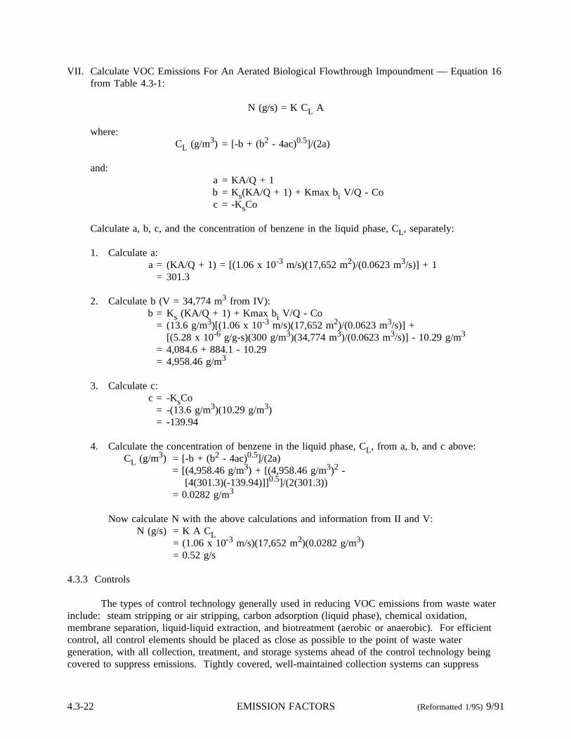
VII. Calculate VOC Emissions For An Aerated Biological Flowthrough Impoundment — Equation 16from Table 4.3-1:
N (g/s) = K CL A
where:CL (g/m3) = [-b + (b2 - 4ac)0.5]/(2a)
and:a = KA/Q + 1b = Ks(KA/Q + 1) + Kmax bi V/Q - Coc = -KsCo
Calculate a, b, c, and the concentration of benzene in the liquid phase, CL, separately:
1. Calculate a:a = (KA/Q + 1) = [(1.06 x 10⁻³ m/s)(17,652 m2)/(0.0623 m3/s)] + 1
= 301.3
2. Calculate b (V = 34,774 m3 from IV):b = Ks (KA/Q + 1) + Kmax bi V/Q - Co
= (13.6 g/m3)[(1.06 x 10-3 m/s)(17,652 m2)/(0.0623 m3/s)] +[(5.28 x 10⁻⁶ g/g-s)(300 g/m3)(34,774 m3)/(0.0623 m3/s)] - 10.29 g/m3
= 4,084.6 + 884.1 - 10.29= 4,958.46 g/m3
3. Calculate c:c = -KsCo
= -(13.6 g/m3)(10.29 g/m3)= -139.94
4. Calculate the concentration of benzene in the liquid phase, CL, from a, b, and c above:CL (g/m3) = [-b + (b2 - 4ac)0.5]/(2a)
= [(4,958.46 g/m3) + [(4,958.46 g/m3)2 -[4(301.3)(-139.94)]]0.5]/(2(301.3))
= 0.0282 g/m3
Now calculate N with the above calculations and information from II and V:N (g/s) = K A CL
= (1.06 x 10⁻³ m/s)(17,652 m2)(0.0282 g/m3)= 0.52 g/s
4.3.3 Controls
The types of control technology generally used in reducing VOC emissions from waste waterinclude: steam stripping or air stripping, carbon adsorption (liquid phase), chemical oxidation,membrane separation, liquid-liquid extraction, and biotreatment (aerobic or anaerobic). For efficientcontrol, all control elements should be placed as close as possible to the point of waste watergeneration, with all collection, treatment, and storage systems ahead of the control technology beingcovered to suppress emissions. Tightly covered, well-maintained collection systems can suppress
4.3-22 EMISSION FACTORS (Reformatted 1/95)9/91
emissions by 95 to 99 percent. However, if there is explosion potential, the components should bevented to a control device such as an incinerator or carbon adsorber.
The following are brief descriptions of the control technology listed above and of anysecondary controls that may need to be considered for fugitive air emissions.
Steam stripping is the fractional distillation of waste water to remove volatile organicconstituents, with the basic operating principle being the direct contact of steam with waste water.The steam provides the heat of vaporization for the more volatile organic constituents. Removalefficiencies vary with volatility and solubility of the organic impurities. For highly volatilecompounds (HLC greater than 10-3 atm-m3/gmol), average VOC removal ranges from 95 to99 percent. For medium-volatility compounds (HLC between 10-5 and 10-3 atm-m3/gmol), averageremoval ranges from 90 to 95 percent. For low-volatility compounds (HLC <10-5 atm-m3/gmol),average removal ranges from less than 50 to 90 percent.
Air stripping involves the contact of waste water and air to strip out volatile organicconstituents. By forcing large volumes of air through contaminated water, the surface area of water incontact with air is greatly increased, resulting in an increase in the transfer rate of the organiccompounds into the vapor phase. Removal efficiencies vary with volatility and solubility of organicimpurities. For highly volatile compounds, average removal ranges from 90 to 99 percent; formedium- to low-volatility compounds, removal ranges from less than 50 to 90 percent.
Steam stripping and air stripping controls most often are vented to a secondary control, such asa combustion device or gas phase carbon adsorber. Combustion devices may include incinerators,boilers, and flares. Vent gases of high fuel value can be used as an alternate fuel. Typically, vent gasis combined with other fuels such as natural gas and fuel oil. If the fuel value is very low, vent gasescan be heated and combined with combustion air. It is important to note that organics such aschlorinated hydrocarbons can emit toxic pollutants when combusted.
Secondary control by gas phase carbon adsorption processes takes advantage of compoundaffinities for activated carbon. The types of gas phase carbon adsorption systems most commonlyused to control VOC are fixed-bed carbon adsorbers and carbon canisters. Fixed-bed carbon adsorbersare used to control continuous organic gas streams with flow rates ranging from 30 to over3000 m3/min. Canisters are much simpler and smaller than fixed-bed systems and are usually installedto control gas flows of less than 3 m3/min.4 Removal efficiencies depend highly on the type ofcompound being removed. Pollutant-specific activated carbon is usually required. Average removalefficiency ranges from 90 to 99 percent.
Like gas phase carbon adsorption, liquid phase carbon adsorption takes advantage ofcompound affinities for activated carbon. Activated carbon is an excellent adsorbent, because of itslarge surface area and because it is usually in granular or powdered form for easy handling. Twotypes of liquid phase carbon adsorption are the fixed-bed and moving-bed systems. The fixed-bedsystem is used primarily for low-flow waste water streams with contact times around 15 minutes, andit is a batch operation (i. e., once the carbon is spent, the system is taken off line). Moving-bedcarbon adsorption systems operate continuously with waste water typically being introduced from thebottom of the column and regenerated carbon from the top (countercurrent flow). Spent carbon iscontinuously removed from the bottom of the bed. Liquid phase carbon adsorption is usually used forlow concentrations of nonvolatile components and for high concentrations of nondegradablecompounds.5 Removal efficiencies depend on whether the compound is adsorbed on activated carbon.Average removal efficiency ranges from 90 to 99 percent.
9/91 (Reformatted 1/95) Evaporation Loss Sources 4.3-23
Chemical oxidation involves a chemical reaction between the organic compound and anoxidant such as ozone, hydrogen peroxide, permanganate, or chlorine dioxide. Ozone is usually addedto the waste water through an ultraviolet-ozone reactor. Permanganate and chlorine dioxide are addeddirectly into the waste water. It is important to note that adding chlorine dioxide can form chlorinatedhydrocarbons in a side reaction. The applicability of this technique depends on the reactivity of theindividual organic compound.
Two types of membrane separation processes are ultrafiltration and reverse osmosis.Ultrafiltration is primarily a physical sieving process driven by a pressure gradient across themembrane. This process separates organic compounds with molecular weights greater than 2000,depending on the size of the membrane pore. Reverse osmosis is the process by which a solvent isforced across a semipermeable membrane because of an osmotic pressure gradient. Selectivity is,therefore, based on osmotic diffusion properties of the compound and on the molecular diameter of thecompound and membrane pores.4
Liquid-liquid extraction as a separation technique involves differences in solubility ofcompounds in various solvents. Contacting a solution containing the desired compound with a solventin which the compound has a greater solubility may remove the compound from the solution. Thistechnology is often used for product and process solvent recovery. Through distillation, the targetcompound is usually recovered, and the solvent reused.
Biotreatment is the aerobic or anaerobic chemical breakdown of organic chemicals bymicroorganisms. Removal of organics by biodegradation is highly dependent on the compound’sbiodegradability, its volatility, and its ability to be adsorbed onto solids. Removal efficiencies rangefrom almost zero to 100 percent. In general, highly volatile compounds such as chlorinatedhydrocarbons and aromatics will biodegrade very little because of their high-volatility, while alcoholsand other compounds soluble in water, as well as low-volatility compounds, can be almost totallybiodegraded in an acclimated system. In the acclimated biotreatment system, the microorganismseasily convert available organics into biological cells, or biomass. This often requires a mixed cultureof organisms, where each organism utilizes the food source most suitable to its metabolism. Theorganisms will starve and the organics will not be biodegraded if a system is not acclimated, i. e., theorganisms cannot metabolize the available food source.
4.3.4 Glossary Of Terms
Basin - an earthen or concrete-lined depression used to hold liquid.
Completely mixed - having the same characteristics and quality throughout or at all times.
Disposal - the act of permanent storage. Flow of liquid into, but not out of a device.
Drain - a device used for the collection of liquid. It may be open to the atmosphere orbe equipped with a seal to prevent emissions of vapors.
Flowthrough - having a continuous flow into and out of a device.
Plug flow - having characteristics and quality not uniform throughout. These will changein the direction the fluid flows, but not perpendicular to the direction of flow(i. e., no axial movement)
4.3-24 EMISSION FACTORS (Reformatted 1/95)9/91

Storage - any device to accept and retain a fluid for the purpose of future discharge.Discontinuity of flow of liquid into and out of a device.
Treatment - the act of improving fluid properties by physical means. The removal ofundesirable impurities from a fluid.
VOC - volatile organic compounds, referring to all organic compounds except thefollowing, which have been shown not to be photochemically reactive:methane, ethane, trichlorotrifluoroethane, methylene chloride,1,1,1,-trichloroethane, trichlorofluoromethane, dichlorodifluoromethane,chlorodifluoromethane, trifluoromethane, dichlorotetrafluoroethane, andchloropentafluoroethane.
9/91 (Reformatted 1/95) Evaporation Loss Sources 4.3-25
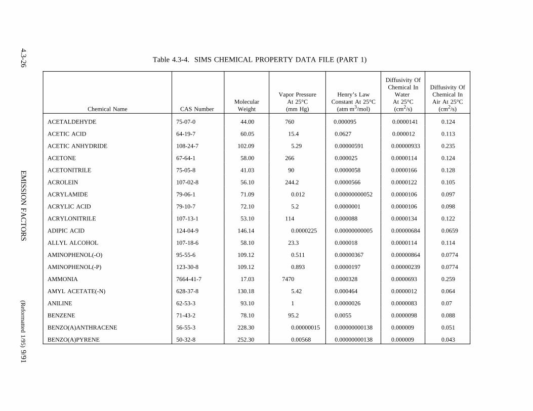
Table 4.3-4. SIMS CHEMICAL PROPERTY DATA FILE (PART 1)
Chemical Name CAS NumberMolecular
Weight
Vapor PressureAt 25°C(mm Hg)
Henry’s LawConstant At 25°C
(atm m3/mol)
Diffusivity OfChemical In
WaterAt 25°C(cm2/s)
Diffusivity OfChemical InAir At 25°C
(cm2/s)
ACETALDEHYDE 75-07-0 44.00 760 0.000095 0.0000141 0.124
ACETIC ACID 64-19-7 60.05 15.4 0.0627 0.000012 0.113
ACETIC ANHYDRIDE 108-24-7 102.09 5.29 0.00000591 0.00000933 0.235
ACETONE 67-64-1 58.00 266 0.000025 0.0000114 0.124
ACETONITRILE 75-05-8 41.03 90 0.0000058 0.0000166 0.128
ACROLEIN 107-02-8 56.10 244.2 0.0000566 0.0000122 0.105
ACRYLAMIDE 79-06-1 71.09 0.012 0.00000000052 0.0000106 0.097
ACRYLIC ACID 79-10-7 72.10 5.2 0.0000001 0.0000106 0.098
ACRYLONITRILE 107-13-1 53.10 114 0.000088 0.0000134 0.122
ADIPIC ACID 124-04-9 146.14 0.0000225 0.00000000005 0.00000684 0.0659
ALLYL ALCOHOL 107-18-6 58.10 23.3 0.000018 0.0000114 0.114
AMINOPHENOL(-O) 95-55-6 109.12 0.511 0.00000367 0.00000864 0.0774
AMINOPHENOL(-P) 123-30-8 109.12 0.893 0.0000197 0.00000239 0.0774
AMMONIA 7664-41-7 17.03 7470 0.000328 0.0000693 0.259
AMYL ACETATE(-N) 628-37-8 130.18 5.42 0.000464 0.0000012 0.064
ANILINE 62-53-3 93.10 1 0.0000026 0.0000083 0.07
BENZENE 71-43-2 78.10 95.2 0.0055 0.0000098 0.088
BENZO(A)ANTHRACENE 56-55-3 228.30 0.00000015 0.00000000138 0.000009 0.051
BENZO(A)PYRENE 50-32-8 252.30 0.00568 0.00000000138 0.000009 0.043
4.3-26E
MIS
SIO
NF
AC
TO
RS
(Reform
atted1/95)9/91

Table 4.3-4 (Part 1) (cont.).
Chemical Name CAS NumberMolecular
Weight
Vapor PressureAt 25°C(mm Hg)
Henry’s LawConstant At 25°C
(atm m3/mol)
Diffusivity OfChemical In
WaterAt 25°C(cm2/s)
Diffusivity OfChemical InAir At 25°C
(cm2/s)
CRESYLIC ACID 1319-77-3 108.00 0.3 0.0000017 0.0000083 0.074
CROTONALDEHYDE 4170-30-0 70.09 30 0.00000154 0.0000102 0.0903
CUMENE (ISOPROPYLBENZENE) 98-82-8 120.20 4.6 0.0146 0.0000071 0.065
CYCLOHEXANE 110-82-7 84.20 100 0.0137 0.0000091 0.0839
CYCLOHEXANOL 108-93-0 100.20 1.22 0.00000447 0.00000831 0.214
CYCLOHEXANONE 108-94-1 98.20 4.8 0.00000413 0.00000862 0.0784
DI-N-OCTYL PHTHALATE 117-84-0 390.62 0 0.137 0.0000041 0.0409
DIBUTYLPHTHALATE 84-74-2 278.30 0.00001 0.00000028 0.0000079 0.0438
DICHLORO(-2)BUTENE(1,4) 764-41-0 125.00 2.87 0.000259 0.00000812 0.0725
DICHLOROBENZENE(1,2) (-O) 95-50-1 147.00 1.5 0.00194 0.0000079 0.069
DICHLOROBENZENE(1,3) (-M) 541-73-1 147.00 2.28 0.00361 0.0000079 0.069
DICHLOROBENZENE(1,4) (-P) 106-46-7 147.00 1.2 0.0016 0.0000079 0.069
DICHLORODIFLUOROMETHANE 75-71-8 120.92 5000 0.401 0.00001 0.0001
DICHLOROETHANE(1,1) 75-34-3 99.00 234 0.00554 0.0000105 0.0914
DICHLOROETHANE(1,2) 107-06-2 99.00 80 0.0012 0.0000099 0.104
DICHLOROETHYLENE(1,2) 156-54-2 96.94 200 0.0319 0.000011 0.0935
DICHLOROPHENOL(2,4) 120-83-2 163.01 0.1 0.0000048 0.0000076 0.0709
DICHLOROPHENOXYACETIC ACID(2,4) 94-75-7 221.00 290 0.0621 0.00000649 0.0588
DICHLOROPROPANE(1,2) 78-87-5 112.99 40 0.0023 0.0000087 0.0782
DIETHYL (N,N) ANILIN 91-66-7 149.23 0.00283 0.0000000574 0.00000587 0.0513
9/91(R
eformatted
1/95)E
vaporationLoss
Sources
4.3-27
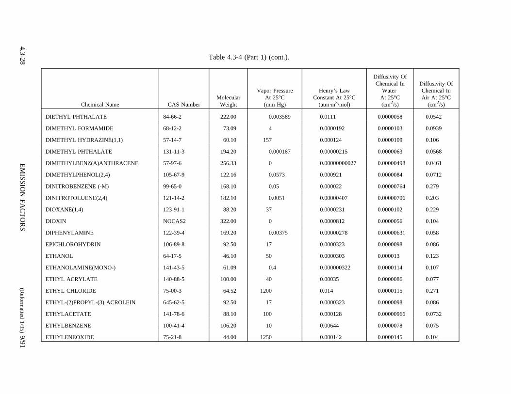
Table 4.3-4 (Part 1) (cont.).
Chemical Name CAS NumberMolecular
Weight
Vapor PressureAt 25°C(mm Hg)
Henry’s LawConstant At 25°C
(atm m3/mol)
Diffusivity OfChemical In
WaterAt 25°C(cm2/s)
Diffusivity OfChemical InAir At 25°C
(cm2/s)
DIETHYL PHTHALATE 84-66-2 222.00 0.003589 0.0111 0.0000058 0.0542
DIMETHYL FORMAMIDE 68-12-2 73.09 4 0.0000192 0.0000103 0.0939
DIMETHYL HYDRAZINE(1,1) 57-14-7 60.10 157 0.000124 0.0000109 0.106
DIMETHYL PHTHALATE 131-11-3 194.20 0.000187 0.00000215 0.0000063 0.0568
DIMETHYLBENZ(A)ANTHRACENE 57-97-6 256.33 0 0.00000000027 0.00000498 0.0461
DIMETHYLPHENOL(2,4) 105-67-9 122.16 0.0573 0.000921 0.0000084 0.0712
DINITROBENZENE (-M) 99-65-0 168.10 0.05 0.000022 0.00000764 0.279
DINITROTOLUENE(2,4) 121-14-2 182.10 0.0051 0.00000407 0.00000706 0.203
DIOXANE(1,4) 123-91-1 88.20 37 0.0000231 0.0000102 0.229
DIOXIN NOCAS2 322.00 0 0.0000812 0.0000056 0.104
DIPHENYLAMINE 122-39-4 169.20 0.00375 0.00000278 0.00000631 0.058
EPICHLOROHYDRIN 106-89-8 92.50 17 0.0000323 0.0000098 0.086
ETHANOL 64-17-5 46.10 50 0.0000303 0.000013 0.123
ETHANOLAMINE(MONO-) 141-43-5 61.09 0.4 0.000000322 0.0000114 0.107
ETHYL ACRYLATE 140-88-5 100.00 40 0.00035 0.0000086 0.077
ETHYL CHLORIDE 75-00-3 64.52 1200 0.014 0.0000115 0.271
ETHYL-(2)PROPYL-(3) ACROLEIN 645-62-5 92.50 17 0.0000323 0.0000098 0.086
ETHYLACETATE 141-78-6 88.10 100 0.000128 0.00000966 0.0732
ETHYLBENZENE 100-41-4 106.20 10 0.00644 0.0000078 0.075
ETHYLENEOXIDE 75-21-8 44.00 1250 0.000142 0.0000145 0.104
4.3-28E
MIS
SIO
NF
AC
TO
RS
(Reform
atted1/95)9/91
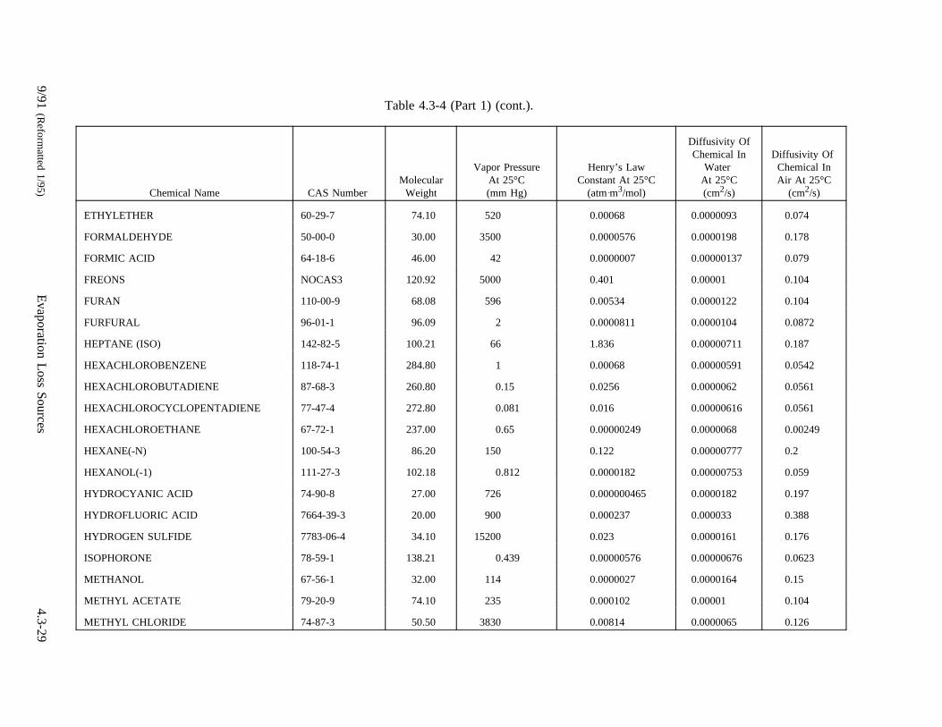
Table 4.3-4 (Part 1) (cont.).
Chemical Name CAS NumberMolecular
Weight
Vapor PressureAt 25°C(mm Hg)
Henry’s LawConstant At 25°C
(atm m3/mol)
Diffusivity OfChemical In
WaterAt 25°C(cm2/s)
Diffusivity OfChemical InAir At 25°C
(cm2/s)
ETHYLETHER 60-29-7 74.10 520 0.00068 0.0000093 0.074
FORMALDEHYDE 50-00-0 30.00 3500 0.0000576 0.0000198 0.178
FORMIC ACID 64-18-6 46.00 42 0.0000007 0.00000137 0.079
FREONS NOCAS3 120.92 5000 0.401 0.00001 0.104
FURAN 110-00-9 68.08 596 0.00534 0.0000122 0.104
FURFURAL 96-01-1 96.09 2 0.0000811 0.0000104 0.0872
HEPTANE (ISO) 142-82-5 100.21 66 1.836 0.00000711 0.187
HEXACHLOROBENZENE 118-74-1 284.80 1 0.00068 0.00000591 0.0542
HEXACHLOROBUTADIENE 87-68-3 260.80 0.15 0.0256 0.0000062 0.0561
HEXACHLOROCYCLOPENTADIENE 77-47-4 272.80 0.081 0.016 0.00000616 0.0561
HEXACHLOROETHANE 67-72-1 237.00 0.65 0.00000249 0.0000068 0.00249
HEXANE(-N) 100-54-3 86.20 150 0.122 0.00000777 0.2
HEXANOL(-1) 111-27-3 102.18 0.812 0.0000182 0.00000753 0.059
HYDROCYANIC ACID 74-90-8 27.00 726 0.000000465 0.0000182 0.197
HYDROFLUORIC ACID 7664-39-3 20.00 900 0.000237 0.000033 0.388
HYDROGEN SULFIDE 7783-06-4 34.10 15200 0.023 0.0000161 0.176
ISOPHORONE 78-59-1 138.21 0.439 0.00000576 0.00000676 0.0623
METHANOL 67-56-1 32.00 114 0.0000027 0.0000164 0.15
METHYL ACETATE 79-20-9 74.10 235 0.000102 0.00001 0.104
METHYL CHLORIDE 74-87-3 50.50 3830 0.00814 0.0000065 0.126
9/91(R
eformatted
1/95)E
vaporationLoss
Sources
4.3-29

Table 4.3-4 (Part 1) (cont.).
Chemical Name CAS NumberMolecular
Weight
Vapor PressureAt 25°C(mm Hg)
Henry’s LawConstant At 25°C
(atm m3/mol)
Diffusivity OfChemical In
WaterAt 25°C(cm2/s)
Diffusivity OfChemical InAir At 25°C
(cm2/s)
METHYL ETHYL KETONE 78-93-3 72.10 100 0.0000435 0.0000098 0.0808
METHYL ISOBUTYL KETONE 108-10-1 100.20 15.7 0.0000495 0.0000078 0.075
METHYL METHACRYLATE 80-62-6 100.10 39 0.000066 0.0000086 0.077
METHYL STYRENE (ALPHA) 98-83-9 118.00 0.076 0.00591 0.0000114 0.264
METHYLENE CHLORIDE 75-09-2 85.00 438 0.00319 0.0000117 0.101
MORPHOLINE 110-91-8 87.12 10 0.0000573 0.0000096 0.091
NAPHTHALENE 91-20-3 128.20 0.23 0.00118 0.0000075 0.059
NITROANILINE(-O) 88-74-4 138.14 0.003 0.0000005 0.000008 0.073
NITROBENZENE 98-95-3 123.10 0.3 0.0000131 0.0000086 0.076
PENTACHLOROBENZENE 608-93-5 250.34 0.0046 0.0073 0.0000063 0.057
PENTACHLOROETHANE 76-01-7 202.30 4.4 0.021 0.0000073 0.066
PENTACHLOROPHENOL 87-86-5 266.40 0.00099 0.0000028 0.0000061 0.056
PHENOL 108-95-2 94.10 0.34 0.000000454 0.0000091 0.082
PHOSGENE 75-44-5 98.92 1390 0.171 0.00000112 0.108
PHTHALIC ACID 100-21-0 166.14 121 0.0132 0.0000068 0.064
PHTHALIC ANHYDRIDE 85-44-9 148.10 0.0015 0.0000009 0.0000086 0.071
PICOLINE(-2) 108-99-6 93.12 10.4 0.000127 0.0000096 0.075
POLYCHLORINATED BIPHENYLS 1336-36-3 290.00 0.00185 0.0004 0.00001 0.104
PROPANOL (ISO) 71-23-8 60.09 42.8 0.00015 0.0000104 0.098
PROPIONALDEHYDE 123-38-6 58.08 300 0.00115 0.0000114 0.102
4.3-30E
MIS
SIO
NF
AC
TO
RS
(Reform
atted1/95)9/91
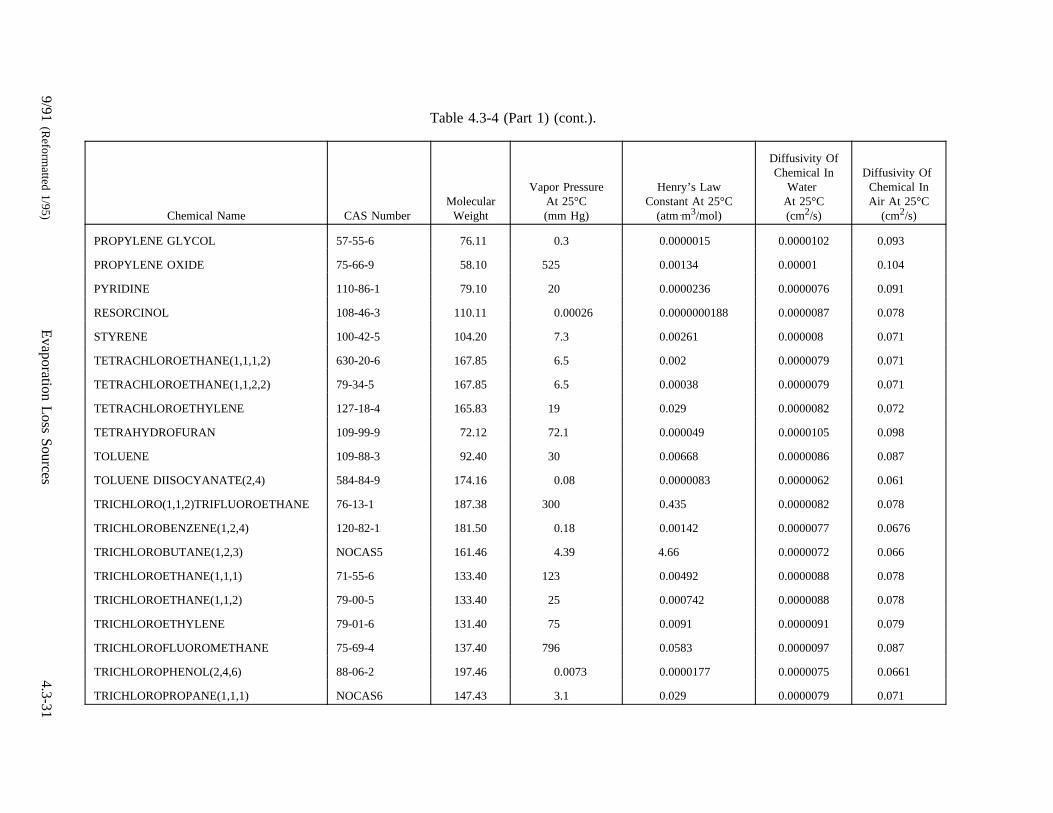
Table 4.3-4 (Part 1) (cont.).
Chemical Name CAS NumberMolecular
Weight
Vapor PressureAt 25°C(mm Hg)
Henry’s LawConstant At 25°C
(atm m3/mol)
Diffusivity OfChemical In
WaterAt 25°C(cm2/s)
Diffusivity OfChemical InAir At 25°C
(cm2/s)
PROPYLENE GLYCOL 57-55-6 76.11 0.3 0.0000015 0.0000102 0.093
PROPYLENE OXIDE 75-66-9 58.10 525 0.00134 0.00001 0.104
PYRIDINE 110-86-1 79.10 20 0.0000236 0.0000076 0.091
RESORCINOL 108-46-3 110.11 0.00026 0.0000000188 0.0000087 0.078
STYRENE 100-42-5 104.20 7.3 0.00261 0.000008 0.071
TETRACHLOROETHANE(1,1,1,2) 630-20-6 167.85 6.5 0.002 0.0000079 0.071
TETRACHLOROETHANE(1,1,2,2) 79-34-5 167.85 6.5 0.00038 0.0000079 0.071
TETRACHLOROETHYLENE 127-18-4 165.83 19 0.029 0.0000082 0.072
TETRAHYDROFURAN 109-99-9 72.12 72.1 0.000049 0.0000105 0.098
TOLUENE 109-88-3 92.40 30 0.00668 0.0000086 0.087
TOLUENE DIISOCYANATE(2,4) 584-84-9 174.16 0.08 0.0000083 0.0000062 0.061
TRICHLORO(1,1,2)TRIFLUOROETHANE 76-13-1 187.38 300 0.435 0.0000082 0.078
TRICHLOROBENZENE(1,2,4) 120-82-1 181.50 0.18 0.00142 0.0000077 0.0676
TRICHLOROBUTANE(1,2,3) NOCAS5 161.46 4.39 4.66 0.0000072 0.066
TRICHLOROETHANE(1,1,1) 71-55-6 133.40 123 0.00492 0.0000088 0.078
TRICHLOROETHANE(1,1,2) 79-00-5 133.40 25 0.000742 0.0000088 0.078
TRICHLOROETHYLENE 79-01-6 131.40 75 0.0091 0.0000091 0.079
TRICHLOROFLUOROMETHANE 75-69-4 137.40 796 0.0583 0.0000097 0.087
TRICHLOROPHENOL(2,4,6) 88-06-2 197.46 0.0073 0.0000177 0.0000075 0.0661
TRICHLOROPROPANE(1,1,1) NOCAS6 147.43 3.1 0.029 0.0000079 0.071
9/91(R
eformatted
1/95)E
vaporationLoss
Sources
4.3-31

Table 4.3-4 (Part 1) (cont.).
Chemical Name CAS NumberMolecular
Weight
Vapor PressureAt 25°C(mm Hg)
Henry’s LawConstant At 25°C
(atm m3/mol)
Diffusivity OfChemical In
WaterAt 25°C(cm2/s)
Diffusivity OfChemical InAir At 25°C
(cm2/s)
TRICHLOROPROPANE(1,2,3) 96-18-4 147.43 3 0.028 0.0000079 0.071
UREA 57-13-6 60.06 6.69 0.000264 0.0000137 0.122
VINYL ACETATE 108-05-4 86.09 115 0.00062 0.0000092 0.085
VINYL CHLORIDE 75-01-4 62.50 2660 0.086 0.0000123 0.106
VINYLIDENE CHLORIDE 75-35-4 97.00 591 0.015 0.0000104 0.09
XYLENE(-M) 1330-20-7 106.17 8 0.0052 0.0000078 0.07
XYLENE(-O) 95-47-6 106.17 7 0.00527 0.00001 0.087
4.3-32E
MIS
SIO
NF
AC
TO
RS
(Reform
atted1/95)9/91

Table 4.3-4. SIMS CHEMICAL PROPERTY DATA FILE (PART 2)
Chemical Name
Antoine’sEquation Vapor
PressureCoefficient
A
Antoine’sEquation Vapor
PressureCoefficient
B
Antoine’sEquation Vapor
PressureCoefficient
C
MaximumBiodegradationRate Constant
(g/g Biomass-s)
Half SaturationConstant(g/m3)
Octanol-WaterPartition
CoefficientAt 25°C
ACETALDEHYDE 8.005 1600.017 291.809 0.0000228944 419.0542 2.69153
ACETIC ACID 7.387 1533.313 222.309 0.0000038889 14.2857 0.48978
ACETIC ANHYDRIDE 7.149 1444.718 199.817 0.0000026944 1.9323 1
ACETONE 7.117 1210.595 229.664 0.0000003611 1.1304 0.57544
ACETONITRILE 7.119 1314.4 230 0.00000425 152.6014 0.45709
ACROLEIN 2.39 0 0 0.0000021667 22.9412 0.81283
ACRYLAMIDE 11.2932 3939.877 273.16 0.00000425 56.2388 6.32182
ACRYLIC ACID 5.652 648.629 154.683 0.0000026944 54.7819 2.04174
ACRYLONITRILE 7.038 1232.53 222.47 0.000005 24 0.12023
ADIPIC ACID 0 0 0 0.0000026944 66.9943 1.20226
ALLYL ALCOHOL 0 0 0 0.0000048872 3.9241 1.47911
AMINOPHENOL(-O) 0 0 0 0.00000425 68.1356 3.81533
AMINOPHENOL(-P) -3.357 699.157 -331.343 0.00000425 68.1356 3.81533
AMMONIA 7.5547 1002.711 247.885 0.00000425 15.3 1
AMYL ACETATE(-N) 0 0 0 0.0000026944 16.1142 51.10801
ANILINE 7.32 1731.515 206.049 0.0000019722 .3381 7.94328
BENZENE 6.905 1211.033 220.79 0.0000052778 13.5714 141.25375
BENZO(A)ANTHRACENE 6.9824 2426.6 156.6 0.0000086389 1.7006 407380.2778
BENZO(A)PYRENE 9.2455 3724.363 273.16 0.0000086389 1.2303 954992.58602
9/91(R
eformatted
1/95)E
vaporationLoss
Sources
4.3-33
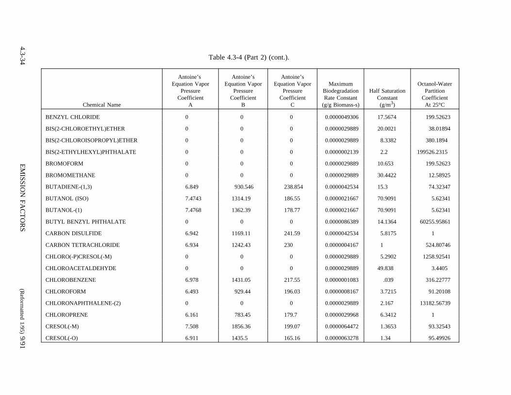
Table 4.3-4 (Part 2) (cont.).
Chemical Name
Antoine’sEquation Vapor
PressureCoefficient
A
Antoine’sEquation Vapor
PressureCoefficient
B
Antoine’sEquation Vapor
PressureCoefficient
C
MaximumBiodegradationRate Constant
(g/g Biomass-s)
Half SaturationConstant(g/m3)
Octanol-WaterPartition
CoefficientAt 25°C
BENZYL CHLORIDE 0 0 0 0.0000049306 17.5674 199.52623
BIS(2-CHLOROETHYL)ETHER 0 0 0 0.0000029889 20.0021 38.01894
BIS(2-CHLOROISOPROPYL)ETHER 0 0 0 0.0000029889 8.3382 380.1894
BIS(2-ETHYLHEXYL)PHTHALATE 0 0 0 0.0000002139 2.2 199526.2315
BROMOFORM 0 0 0 0.0000029889 10.653 199.52623
BROMOMETHANE 0 0 0 0.0000029889 30.4422 12.58925
BUTADIENE-(1,3) 6.849 930.546 238.854 0.0000042534 15.3 74.32347
BUTANOL (ISO) 7.4743 1314.19 186.55 0.0000021667 70.9091 5.62341
BUTANOL-(1) 7.4768 1362.39 178.77 0.0000021667 70.9091 5.62341
BUTYL BENZYL PHTHALATE 0 0 0 0.0000086389 14.1364 60255.95861
CARBON DISULFIDE 6.942 1169.11 241.59 0.0000042534 5.8175 1
CARBON TETRACHLORIDE 6.934 1242.43 230 0.0000004167 1 524.80746
CHLORO(-P)CRESOL(-M) 0 0 0 0.0000029889 5.2902 1258.92541
CHLOROACETALDEHYDE 0 0 0 0.0000029889 49.838 3.4405
CHLOROBENZENE 6.978 1431.05 217.55 0.0000001083 .039 316.22777
CHLOROFORM 6.493 929.44 196.03 0.0000008167 3.7215 91.20108
CHLORONAPHTHALENE-(2) 0 0 0 0.0000029889 2.167 13182.56739
CHLOROPRENE 6.161 783.45 179.7 0.0000029968 6.3412 1
CRESOL(-M) 7.508 1856.36 199.07 0.0000064472 1.3653 93.32543
CRESOL(-O) 6.911 1435.5 165.16 0.0000063278 1.34 95.49926
4.3-34E
MIS
SIO
NF
AC
TO
RS
(Reform
atted1/95)9/91
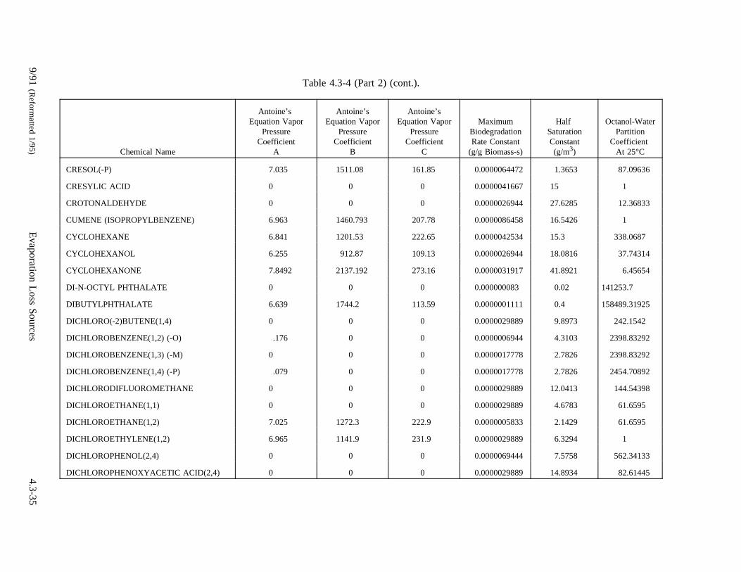
Table 4.3-4 (Part 2) (cont.).
Chemical Name
Antoine’sEquation Vapor
PressureCoefficient
A
Antoine’sEquation Vapor
PressureCoefficient
B
Antoine’sEquation Vapor
PressureCoefficient
C
MaximumBiodegradationRate Constant
(g/g Biomass-s)
HalfSaturationConstant(g/m3)
Octanol-WaterPartition
CoefficientAt 25°C
CRESOL(-P) 7.035 1511.08 161.85 0.0000064472 1.3653 87.09636
CRESYLIC ACID 0 0 0 0.0000041667 15 1
CROTONALDEHYDE 0 0 0 0.0000026944 27.6285 12.36833
CUMENE (ISOPROPYLBENZENE) 6.963 1460.793 207.78 0.0000086458 16.5426 1
CYCLOHEXANE 6.841 1201.53 222.65 0.0000042534 15.3 338.0687
CYCLOHEXANOL 6.255 912.87 109.13 0.0000026944 18.0816 37.74314
CYCLOHEXANONE 7.8492 2137.192 273.16 0.0000031917 41.8921 6.45654
DI-N-OCTYL PHTHALATE 0 0 0 0.000000083 0.02 141253.7
DIBUTYLPHTHALATE 6.639 1744.2 113.59 0.0000001111 0.4 158489.31925
DICHLORO(-2)BUTENE(1,4) 0 0 0 0.0000029889 9.8973 242.1542
DICHLOROBENZENE(1,2) (-O) .176 0 0 0.0000006944 4.3103 2398.83292
DICHLOROBENZENE(1,3) (-M) 0 0 0 0.0000017778 2.7826 2398.83292
DICHLOROBENZENE(1,4) (-P) .079 0 0 0.0000017778 2.7826 2454.70892
DICHLORODIFLUOROMETHANE 0 0 0 0.0000029889 12.0413 144.54398
DICHLOROETHANE(1,1) 0 0 0 0.0000029889 4.6783 61.6595
DICHLOROETHANE(1,2) 7.025 1272.3 222.9 0.0000005833 2.1429 61.6595
DICHLOROETHYLENE(1,2) 6.965 1141.9 231.9 0.0000029889 6.3294 1
DICHLOROPHENOL(2,4) 0 0 0 0.0000069444 7.5758 562.34133
DICHLOROPHENOXYACETIC ACID(2,4) 0 0 0 0.0000029889 14.8934 82.61445
9/91(R
eformatted
1/95)E
vaporationLoss
Sources
4.3-35
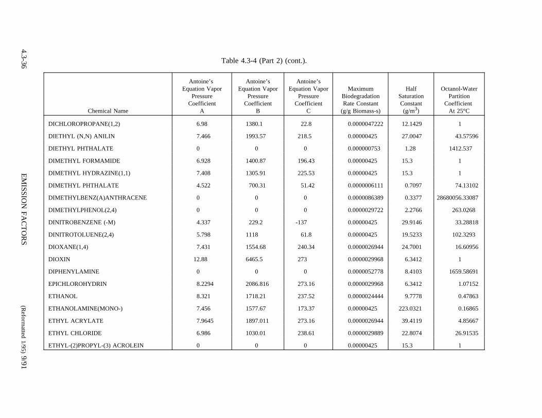
Table 4.3-4 (Part 2) (cont.).
Chemical Name
Antoine’sEquation Vapor
PressureCoefficient
A
Antoine’sEquation Vapor
PressureCoefficient
B
Antoine’sEquation Vapor
PressureCoefficient
C
MaximumBiodegradationRate Constant
(g/g Biomass-s)
HalfSaturationConstant(g/m3)
Octanol-WaterPartition
CoefficientAt 25°C
DICHLOROPROPANE(1,2) 6.98 1380.1 22.8 0.0000047222 12.1429 1
DIETHYL (N,N) ANILIN 7.466 1993.57 218.5 0.00000425 27.0047 43.57596
DIETHYL PHTHALATE 0 0 0 0.000000753 1.28 1412.537
DIMETHYL FORMAMIDE 6.928 1400.87 196.43 0.00000425 15.3 1
DIMETHYL HYDRAZINE(1,1) 7.408 1305.91 225.53 0.00000425 15.3 1
DIMETHYL PHTHALATE 4.522 700.31 51.42 0.0000006111 0.7097 74.13102
DIMETHYLBENZ(A)ANTHRACENE 0 0 0 0.0000086389 0.3377 28680056.33087
DIMETHYLPHENOL(2,4) 0 0 0 0.0000029722 2.2766 263.0268
DINITROBENZENE (-M) 4.337 229.2 -137 0.00000425 29.9146 33.28818
DINITROTOLUENE(2,4) 5.798 1118 61.8 0.00000425 19.5233 102.3293
DIOXANE(1,4) 7.431 1554.68 240.34 0.0000026944 24.7001 16.60956
DIOXIN 12.88 6465.5 273 0.0000029968 6.3412 1
DIPHENYLAMINE 0 0 0 0.0000052778 8.4103 1659.58691
EPICHLOROHYDRIN 8.2294 2086.816 273.16 0.0000029968 6.3412 1.07152
ETHANOL 8.321 1718.21 237.52 0.0000024444 9.7778 0.47863
ETHANOLAMINE(MONO-) 7.456 1577.67 173.37 0.00000425 223.0321 0.16865
ETHYL ACRYLATE 7.9645 1897.011 273.16 0.0000026944 39.4119 4.85667
ETHYL CHLORIDE 6.986 1030.01 238.61 0.0000029889 22.8074 26.91535
ETHYL-(2)PROPYL-(3) ACROLEIN 0 0 0 0.00000425 15.3 1
4.3-36E
MIS
SIO
NF
AC
TO
RS
(Reform
atted1/95)9/91
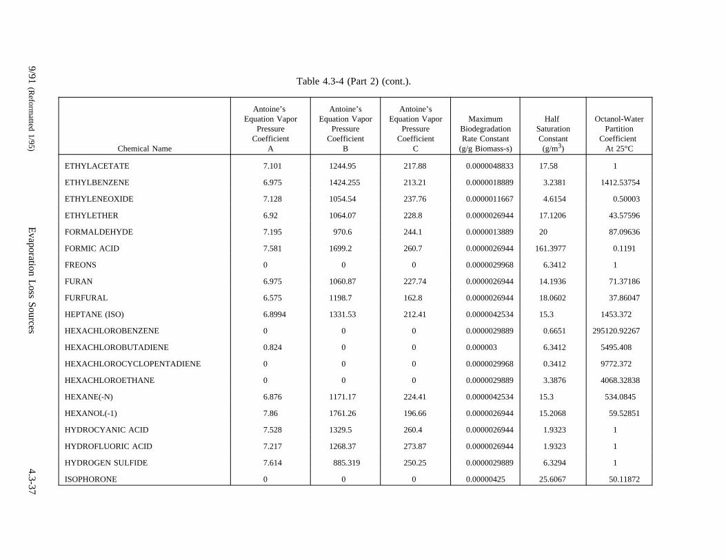
Table 4.3-4 (Part 2) (cont.).
Chemical Name
Antoine’sEquation Vapor
PressureCoefficient
A
Antoine’sEquation Vapor
PressureCoefficient
B
Antoine’sEquation Vapor
PressureCoefficient
C
MaximumBiodegradationRate Constant
(g/g Biomass-s)
HalfSaturationConstant(g/m3)
Octanol-WaterPartition
CoefficientAt 25°C
ETHYLACETATE 7.101 1244.95 217.88 0.0000048833 17.58 1
ETHYLBENZENE 6.975 1424.255 213.21 0.0000018889 3.2381 1412.53754
ETHYLENEOXIDE 7.128 1054.54 237.76 0.0000011667 4.6154 0.50003
ETHYLETHER 6.92 1064.07 228.8 0.0000026944 17.1206 43.57596
FORMALDEHYDE 7.195 970.6 244.1 0.0000013889 20 87.09636
FORMIC ACID 7.581 1699.2 260.7 0.0000026944 161.3977 0.1191
FREONS 0 0 0 0.0000029968 6.3412 1
FURAN 6.975 1060.87 227.74 0.0000026944 14.1936 71.37186
FURFURAL 6.575 1198.7 162.8 0.0000026944 18.0602 37.86047
HEPTANE (ISO) 6.8994 1331.53 212.41 0.0000042534 15.3 1453.372
HEXACHLOROBENZENE 0 0 0 0.0000029889 0.6651 295120.92267
HEXACHLOROBUTADIENE 0.824 0 0 0.000003 6.3412 5495.408
HEXACHLOROCYCLOPENTADIENE 0 0 0 0.0000029968 0.3412 9772.372
HEXACHLOROETHANE 0 0 0 0.0000029889 3.3876 4068.32838
HEXANE(-N) 6.876 1171.17 224.41 0.0000042534 15.3 534.0845
HEXANOL(-1) 7.86 1761.26 196.66 0.0000026944 15.2068 59.52851
HYDROCYANIC ACID 7.528 1329.5 260.4 0.0000026944 1.9323 1
HYDROFLUORIC ACID 7.217 1268.37 273.87 0.0000026944 1.9323 1
HYDROGEN SULFIDE 7.614 885.319 250.25 0.0000029889 6.3294 1
ISOPHORONE 0 0 0 0.00000425 25.6067 50.11872
9/91(R
eformatted
1/95)E
vaporationLoss
Sources
4.3-37
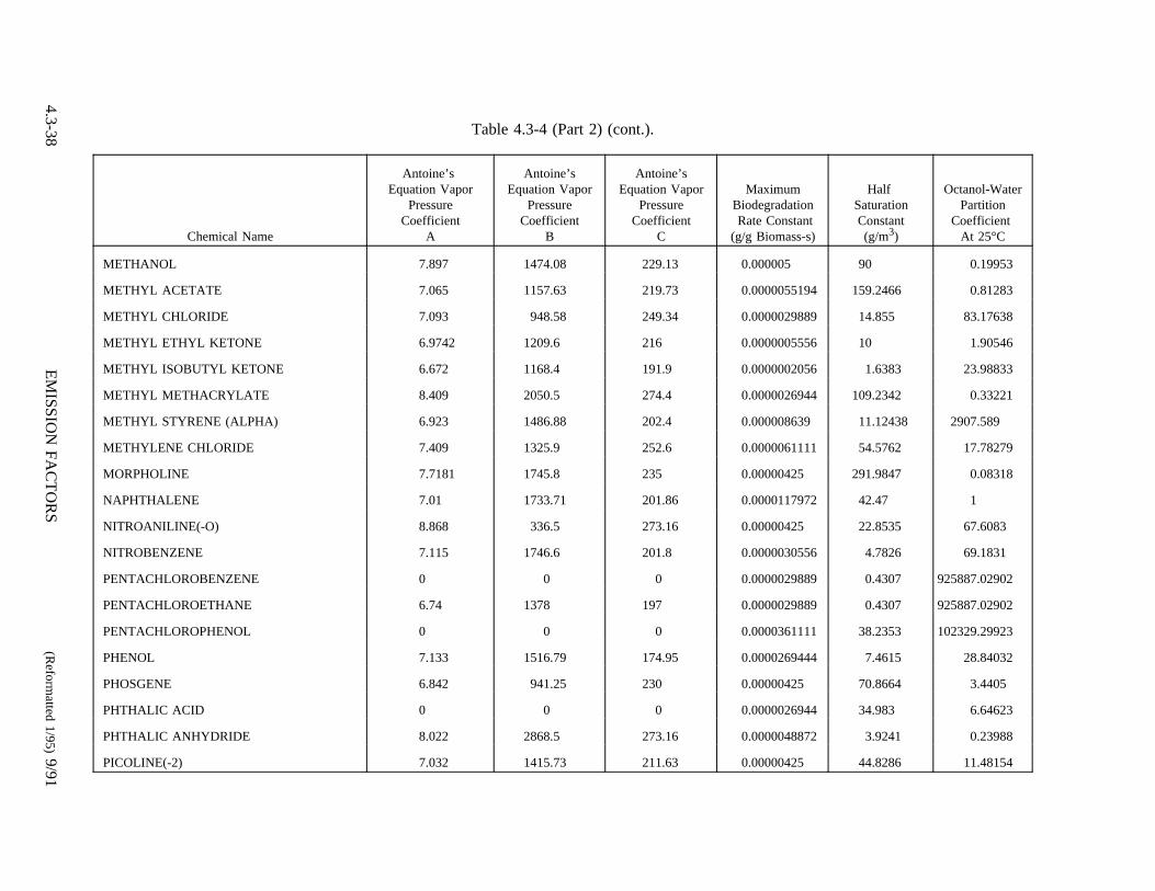
Table 4.3-4 (Part 2) (cont.).
Chemical Name
Antoine’sEquation Vapor
PressureCoefficient
A
Antoine’sEquation Vapor
PressureCoefficient
B
Antoine’sEquation Vapor
PressureCoefficient
C
MaximumBiodegradationRate Constant
(g/g Biomass-s)
HalfSaturationConstant(g/m3)
Octanol-WaterPartition
CoefficientAt 25°C
METHANOL 7.897 1474.08 229.13 0.000005 90 0.19953
METHYL ACETATE 7.065 1157.63 219.73 0.0000055194 159.2466 0.81283
METHYL CHLORIDE 7.093 948.58 249.34 0.0000029889 14.855 83.17638
METHYL ETHYL KETONE 6.9742 1209.6 216 0.0000005556 10 1.90546
METHYL ISOBUTYL KETONE 6.672 1168.4 191.9 0.0000002056 1.6383 23.98833
METHYL METHACRYLATE 8.409 2050.5 274.4 0.0000026944 109.2342 0.33221
METHYL STYRENE (ALPHA) 6.923 1486.88 202.4 0.000008639 11.12438 2907.589
METHYLENE CHLORIDE 7.409 1325.9 252.6 0.0000061111 54.5762 17.78279
MORPHOLINE 7.7181 1745.8 235 0.00000425 291.9847 0.08318
NAPHTHALENE 7.01 1733.71 201.86 0.0000117972 42.47 1
NITROANILINE(-O) 8.868 336.5 273.16 0.00000425 22.8535 67.6083
NITROBENZENE 7.115 1746.6 201.8 0.0000030556 4.7826 69.1831
PENTACHLOROBENZENE 0 0 0 0.0000029889 0.4307 925887.02902
PENTACHLOROETHANE 6.74 1378 197 0.0000029889 0.4307 925887.02902
PENTACHLOROPHENOL 0 0 0 0.0000361111 38.2353 102329.29923
PHENOL 7.133 1516.79 174.95 0.0000269444 7.4615 28.84032
PHOSGENE 6.842 941.25 230 0.00000425 70.8664 3.4405
PHTHALIC ACID 0 0 0 0.0000026944 34.983 6.64623
PHTHALIC ANHYDRIDE 8.022 2868.5 273.16 0.0000048872 3.9241 0.23988
PICOLINE(-2) 7.032 1415.73 211.63 0.00000425 44.8286 11.48154
4.3-38E
MIS
SIO
NF
AC
TO
RS
(Reform
atted1/95)9/91

Table 4.3-4 (Part 2) (cont.).
Chemical Name
Antoine’sEquation Vapor
PressureCoefficient
A
Antoine’sEquation Vapor
PressureCoefficient
B
Antoine’sEquation Vapor
PressureCoefficient
C
MaximumBiodegradationRate Constant
(g/g Biomass-s)Half Saturation
Constant(g/m3)
Octanol-WaterPartition
CoefficientAt 25°C
POLYCHLORINATED BIPHENYLS 0 0 0 0.000005278 20 1
PROPANOL (ISO) 8.117 1580.92 219.61 0.0000041667 200 0.69183
PROPIONALDEHYDE 16.2315 2659.02 -44.15 0.0000026944 39.2284 4.91668
PROPYLENE GLYCOL 8.2082 2085.9 203.5396 0.0000026944 109.3574 0.33141
PROPYLENE OXIDE 8.2768 1656.884 273.16 0.0000048872 3.9241 1
PYRIDINE 7.041 1373.8 214.98 0.0000097306 146.9139 4.46684
RESORCINOL 6.9243 1884.547 186.0596 0.0000026944 35.6809 6.30957
STYRENE 7.14 1574.51 224.09 0.0000086389 282.7273 1445.43977
TETRACHLOROETHANE(1,1,1,2) 6.898 1365.88 209.74 0.0000029889 6.3294 1
TETRACHLOROETHANE(1,1,2,2) 6.631 1228.1 179.9 0.0000017222 9.1176 363.07805
TETRACHLOROETHYLENE 6.98 1386.92 217.53 0.0000017222 9.1176 398.10717
TETRAHYDROFURAN 6.995 1202.29 226.25 0.0000026944 20.3702 27.58221
TOLUENE 6.954 1344.8 219.48 0.0000204111 30.6167 489.77882
TOLUENE DIISOCYANATE(2,4) 0 0 0 0.00000425 15.3 1
TRICHLORO(1,1,2)TRIFLUOROETHANE 6.88 1099.9 227.5 0.0000029889 3.3876 4068.32838
TRICHLOROBENZENE(1,2,4) 0 0 0 0.0000029889 2.4495 9549.92586
TRICHLOROBUTANE(1,2,3) 0 0 0 0.0000029968 6.3412 1450901.06626
TRICHLOROETHANE(1,1,1) 8.643 2136.6 302.8 0.0000009722 4.7297 309.02954
TRICHLOROETHANE(1,1,2) 6.951 1314.41 209.2 0.0000009722 4.7297 1
9/91(R
eformatted
1/95)E
vaporationLoss
Sources
4.3-39
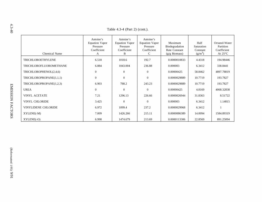
Table 4.3-4 (Part 2) (cont.).
Chemical Name
Antoine’sEquation Vapor
PressureCoefficient
A
Antoine’sEquation Vapor
PressureCoefficient
B
Antoine’sEquation Vapor
PressureCoefficient
C
MaximumBiodegradationRate Constant(g/g Biomass)
HalfSaturationConstant(g/m3)
Octanol-WaterPartition
CoefficientAt 25°C
TRICHLOROETHYLENE 6.518 1018.6 192.7 0.0000010833 4.4318 194.98446
TRICHLOROFLUOROMETHANE 6.884 1043.004 236.88 0.000003 6.3412 338.8441
TRICHLOROPHENOL(2,4,6) 0 0 0 0.00000425 58.8462 4897.78819
TRICHLOROPROPANE(1,1,1) 0 0 0 0.0000029889 10.7719 193.7827
TRICHLOROPROPANE(1,2,3) 6.903 788.2 243.23 0.0000029889 10.7719 193.7827
UREA 0 0 0 0.00000425 4.8169 4068.32838
VINYL ACETATE 7.21 1296.13 226.66 0.0000026944 31.8363 8.51722
VINYL CHLORIDE 3.425 0 0 0.000003 6.3412 1.14815
VINYLIDENE CHLORIDE 6.972 1099.4 237.2 0.0000029968 6.3412 1
XYLENE(-M) 7.009 1426.266 215.11 0.0000086389 14.0094 1584.89319
XYLENE(-O) 6.998 1474.679 213.69 0.0000113306 22.8569 891.25094
4.3-40E
MIS
SIO
NF
AC
TO
RS
(Reform
atted1/95)9/91
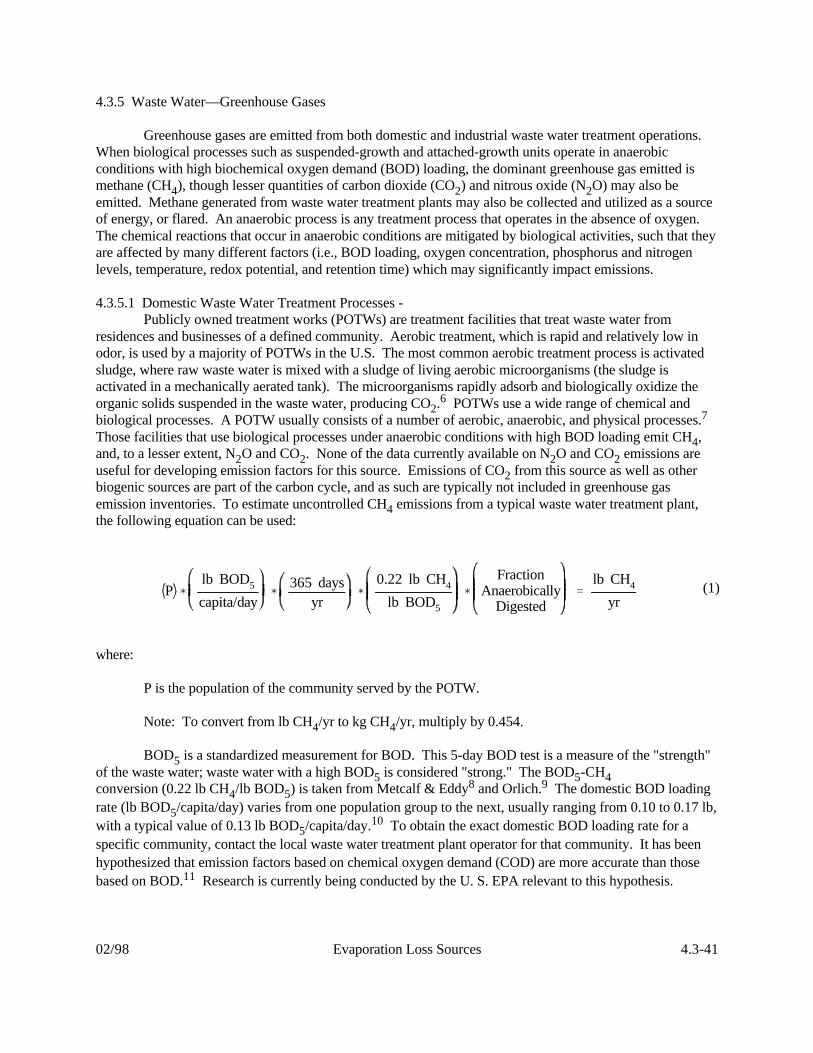
P (lb BOD5
capita/day(
365 daysyr
(0.22 lb CH4
lb BOD5
(
FractionAnaerobically
Digested'
lb CH4
yr
02/98 Evaporation Loss Sources 4.3-41
(1)
4.3.5 Waste Water—Greenhouse Gases
Greenhouse gases are emitted from both domestic and industrial waste water treatment operations. When biological processes such as suspended-growth and attached-growth units operate in anaerobicconditions with high biochemical oxygen demand (BOD) loading, the dominant greenhouse gas emitted ismethane (CH ), though lesser quantities of carbon dioxide (CO ) and nitrous oxide (N O) may also be4 2 2emitted. Methane generated from waste water treatment plants may also be collected and utilized as a sourceof energy, or flared. An anaerobic process is any treatment process that operates in the absence of oxygen. The chemical reactions that occur in anaerobic conditions are mitigated by biological activities, such that theyare affected by many different factors (i.e., BOD loading, oxygen concentration, phosphorus and nitrogenlevels, temperature, redox potential, and retention time) which may significantly impact emissions.
4.3.5.1 Domestic Waste Water Treatment Processes -Publicly owned treatment works (POTWs) are treatment facilities that treat waste water from
residences and businesses of a defined community. Aerobic treatment, which is rapid and relatively low inodor, is used by a majority of POTWs in the U.S. The most common aerobic treatment process is activatedsludge, where raw waste water is mixed with a sludge of living aerobic microorganisms (the sludge isactivated in a mechanically aerated tank). The microorganisms rapidly adsorb and biologically oxidize theorganic solids suspended in the waste water, producing CO . POTWs use a wide range of chemical and2
6
biological processes. A POTW usually consists of a number of aerobic, anaerobic, and physical processes. 7
Those facilities that use biological processes under anaerobic conditions with high BOD loading emit CH ,4and, to a lesser extent, N O and CO . None of the data currently available on N O and CO emissions are2 2 2 2useful for developing emission factors for this source. Emissions of CO from this source as well as other2biogenic sources are part of the carbon cycle, and as such are typically not included in greenhouse gasemission inventories. To estimate uncontrolled CH emissions from a typical waste water treatment plant,4the following equation can be used:
where:
P is the population of the community served by the POTW.
Note: To convert from lb CH /yr to kg CH /yr, multiply by 0.454.4 4
BOD is a standardized measurement for BOD. This 5-day BOD test is a measure of the "strength"5of the waste water; waste water with a high BOD is considered "strong." The BOD -CH 5 5 4conversion (0.22 lb CH /lb BOD ) is taken from Metcalf & Eddy and Orlich. The domestic BOD loading4 5
8 9
rate (lb BOD /capita/day) varies from one population group to the next, usually ranging from 0.10 to 0.17 lb,5with a typical value of 0.13 lb BOD /capita/day. To obtain the exact domestic BOD loading rate for a5
10
specific community, contact the local waste water treatment plant operator for that community. It has beenhypothesized that emission factors based on chemical oxygen demand (COD) are more accurate than thosebased on BOD. Research is currently being conducted by the U. S. EPA relevant to this hypothesis.11

(P) ( 1.56lb CH4
capita/yr' lb
CH4
yr
QI (lb BOD5
ft 3 wastewater(
0.22 lb CH4
lb BOD5
(
FractionAnaerobically
Digested(
365 daysyr
'lb CH4
yr
4.3-42 EMISSION FACTORS 02/98
(2)
(3)
The fraction of the domestic waste water treated anaerobically is calculated by considering whichtreatment processes are anaerobic and what percent of the total hydraulic retention time the waste waterspends in these treatment processes. This fraction is dependent on the treatment processes used and theoperating conditions of a specific plant. This information can also be provided by contacting local wastewater treatment plant operators. If treatment activity data are not available from local wastewater treatmentplant operators, a default value of 15 percent of domestic water treated anaerobically may also be used. A12
default value of 15 percent is also recommended in the Intergovernmental Panel on Climate Change (IPCC)Greenhouse Gas Inventory Reference Manual.13
If a BOD value of 0.13 lb BOD is assumed, the IPCC assumption is used that 5 515 percent of waste water is anaerobically digested, and none of the gas is recovered for energy or flared, thenequation 1 reduces to the following equation:
4.3.5.2 Industrial Waste Water Treatment Processes -An industrial waste water system uses unit processes similar to those found in POTWs. Such a
treatment system may discharge into a water body or may pretreat the waste water for discharge into a sewersystem leading to a POTW. To estimate uncontrolled CH methane emissions from a typical industrial waste4water treatment plant the following equation can be used:
where:Q = daily waste water flow (ft /day).I
3
Flow rates for individual industrial waste water treatment facilities (Q ) can be provided by theIoperator of the industrial waste water treatment plant or by reviewing a facility's National Pollution DischargeElimination System (NPDES) discharge permit.
Industrial BOD loading rates (lb BOD /ft waste water) vary depending upon the source of the waste53
water contamination. Some contaminants have very high BOD , such as contaminants in food and beverage5manufacturers' waste water. Table 4.3-5 provides a list of typical industrial BOD loading rates for majorindustrial sources. To obtain the exact BOD loading rate for a specific facility, contact the facility's wastewater treatment plant operator or review the facility's NPDES discharge permit.

02/98 Evaporation Loss Sources 4.3-43
The fraction of the industrial waste water treated anaerobically is dependent on the treatmentprocesses used in specific plants. The composition of an industrial waste stream is more diverse thanmunicipal wastewater. The difference makes it very difficult to provide a default fraction of anaerobicallytreated wastewater that would be representative of facilities in a specific inventory area. This information canalso be provided by contacting individual waste water treatment plant operators.
4.3.5.3 ControlsWaste water treatment plant operators (domestic as well as industrial) can also provide information
on gas recovery and utilization. If a gas recovery system is in place, uncontrolled CH emissions estimates4should be adjusted based on operator estimates of the efficiency of the gas collection system and thedestruction of the collected gas. For more information on control efficiencies, see Section 4.3.3.
4.3.6 Updates Since the Fifth Edition
The Fifth Edition was released in January 1995. In February 1998, this section was revised by theaddition of 4.3.5 which addresses Greenhouse Gas emissions. The revisions made in February 1998 are to beincluded in Supplement D.

4.3-44 EMISSION FACTORS 02/98
Table 4.3-5. BIOCHEMICAL OXYGEN DEMAND (BOD) ESTIMATES FOR VARIOUSINDUSTRIAL WASTE WATERS
Industry BOD (lb/ft ) Number Range53 a
Reference
Fertilizer 0.04 14 0.03-0.05b
Food andbeverages Beer 5.31 15 4.99-5.62c
Beet sugar 0.41 15, 16 0.34-0.47c
Butter 0.19 17 Cane sugar 0.08 15 0.07-0.09c
Cereals 0.06 18 Cheese 1.9 17Fruits and 40.27 15 Average of BOD values for processing 35 differentvegetables fruits an vegetables. The BOD values ranged fromd
4.370 to 1747.979 lbs/ft . For the BOD value it35
was assumed that biodegradation was high such thatthe BOD value was considered to be 75% of the5BOD value.
Meats 1.3 19 -- Milk 7.6 15 6.24-8.93c
Wine 8.43 15 7.49-9.36c
Iron and steel 0.04 14 0.03-0.05b
Non-ferrous 0.04 14 0.03-0.05metals
b
Petroleum 0.25 14 Average of values reported in Carmichael andrefining Strzepek (1987). (Petrochemical)Pharmaceutical 0.08 14 0.07-0.09c
Pulp and paper 0.17 14, 20 0.14-0.19 Rubber 0.04 14 0.03-0.05b
Textiles 0.04 14 0.03-0.05c
To convert lb/ft to kg/m multiply by 16.0185.a 3 3
A BOD value was not provided in the literature. The range of BOD values was derived from the ultimateb5 5
BOD value from the textile industry, which should have a similar, relatively small value. BOD is 55 to 755percent of ultimate BOD, depending on the biodegradability of the waste stream. The midpoint of theextrapolated range is presented in the second column as BOD .5A range of values is given for BOD because a specific BOD value was not provided in the literature. Thec
5 5range of BOD values was derived from the ultimate BOD value from the literature. BOD is 55 to 755 5percent of ultimate BOD, depending on the biodegradability of the waste stream. If the waste streamcontains a large amount of material that does not biodegrade easily, then a value closer to the lower valueshould be used. If the waste stream contains a large amount of material that does biodegrade easily, then avalue closer to the higher value should be used. If it is unclear how biodegradable the material is, andBOD data for a specific facility is not available, then a value at the midpoint of the range should be used. 5The midpoint of the range is presented in the second column as BOD . 5For a more complete list of BOD values see reference 15.d
5

02/98 Evaporation Loss Sources 4.3-45
References For Section 4.3
1. Hazardous Waste Treatment, Storage, And Disposal Facilities (TSDF) — Air Emission Models,EPA-450/3-87-026, U. S. Environmental Protection Agency, Research Triangle Park, NC,April 1989.
2. Waste Water Treatment Compound Property Processor Air Emissions Estimator (WATER 7), U. S.Environmental Protection Agency, Research Triangle Park, NC, available early 1992.
3. Evaluation Of Test Method For Measuring Biodegradation Rates Of Volatile Organics, Draft,EPA Contract No. 68-D90055, Entropy Environmental, Research Triangle Park, NC,September 1989.
4. Industrial Waste Water Volatile Organic Compound Emissions — Background Information ForBACT/LAER Determinations, EPA-450/3-90-004, U. S. Environmental Protection Agency,Research Triangle Park, NC, January 1990.
5. Evan K. Nyer, Ground Water Treatment Technology, Van Nostrand Reinhold Company, New York,1985.
6. J. Mangino and L. Sutton. Evaluation of Greenhouse Gas Emissions From Wastewater TreatmentSystems. Contract No. 68-D1-0117, Work Assignment 22, U. S. Environmental Protection Agency,Office of Research and Development, Air and Energy Engineering Research Laboratory, ResearchTriangle Park, NC. April 1992.
7. L.C. Huff. Wastewater Methane Emission Estimates--Report to Congress. ContractNo. 68-D1-0117. U. S. Environmental Protection Agency, Office of Research and Development, Airand Energy Engineering Research Laboratory, Research Triangle Park, NC. July 1992.
8. Metcalf & Eddy, Inc., Waste Water Engineering: Treatment, Disposal, And Reuse, McGraw-HillBook Company, p. 621, 1979.
9. Dr. J. Orlich, "Methane Emissions From Landfill Sites And Waste Water Lagoons", Presented inMethane Emissions And Opportunities For Control, 1990.
10. Viessman, Jr. and M.J. Hammer. 1985. Water Supply And Pollution Control. Harper & RowPublishers, New York, NY.
11. U. S. Environmental Protection Agency. International Anthropogenic Methane Emissions Reportto Congress. Office of Policy Planning and Evaluation, EPA 230-R-93-010. 1994.
12. M.J. Lexmond and G. Zeeman. Potential Of Uncontrolled Anaerobic Wastewater Treatment InOrder To Reduce Global Emissions Of The Greenhouse Gases Methane And Carbon Dioxide.
4.3-46 EMISSION FACTORS 02/98
Department of Environmental Technology, Agricultural University of Wageningen, the Netherlands. Report Number 95-1. 1995.
13. Intergovernmental Panel on Climate Control, Greenhouse Gas Inventory Reference Manual, Vol. 3,IPCC/OECD, p. 6.28, 1994.
14. J. B. Carmichael and K.M. Strzepek, Industrial Water Use And Treatment Practices, UnitedNations Industrial Development Organization, Cassell Tycooly, Philadelphia, PA, pp. 33, 36, 49, 67and 85, 1987.
15. D. Barnes, et al., "Surveys In Industrial Waste Water Treatment", Vol. 1, Food And AlliedIndustries, Pitman Publishing Inc., Marshfield, Massachusetts, pp. 12, 73, 213 and 316, 1984.
16. Development Document For Effluent Limitations Guidelines And New Source PerformanceStandards For The Beet Sugar Processing Subcategory Of The Sugar Processing Point SourceCategory, EPA 40/1-74/002b, U. S. Environmental Protection Agency, Effluent GuidelinesDivision, Office Of Waste And Hazardous Materials, Washington, DC, January 1974.
17. Development Document For Effluent Limitations Guidelines And New Source PerformanceStandards For The Dairy Product Processing Point Source Category, EPA 440/1-74/021a, U. S. Environmental Protection Agency, Effluent Guidelines Division, Office Of Waste AndHazardous Materials, Washington, DC, p. 59, May 1974.
18. Development Document For Effluent Limitations Guidelines And New Source PerformanceStandards For The Animal Feed, Breakfast Cereal, And Wheat Starch Segments Of The GrainMills Points Source Category, EPA 440/1-74/039a, U. S. Environmental Protection Agency,Effluent Guidelines Division, Office Of Waste And Hazardous Materials, Washington, DC, pp.39-40, December 1974.
19. Development Document For Effluent Limitations Guidelines And New Source PerformanceStandards For The Rendering Segment Of The Meat Products And Rendering Processing PointSource Category, EPA 400/1-4/031d, U. S. Environmental Protection Agency, Effluent GuidelinesDivision, Office of Waste And Hazardous Materials, Washington, DC, pp. 58, 60, January 1975.
20. E. R. Hall (editor), "Anaerobic Treatment For Pulp And Paper Waste Waters", Anaerobic TreatmentOf Industrial Waste Water, Noyes Data Corporation, Park Ridge, New Jersey pp. 15-22, 1988.