Increasing Scalability in Algorithms for Centralized and Decentralized POMDPs
Journal of Artificial Intelligence Research 27 (2006) 335-380 Submitted 05/06; published 11/06
Anytime Point-Based Approximations for Large POMDPs
Joelle Pineau [email protected]
School of Computer ScienceMcGill UniversityMontreal QC, H3A 2A7 CANADAGeoffrey Gordon [email protected]
Machine Learning DepartmentCarnegie Mellon UniversityPittsburgh PA, 15232 USASebastian Thrun [email protected]
Computer Science DepartmentStanford UniversityStanford CA, 94305 USA
AbstractThe Partially Observable Markov Decision Process has long been recognized as a rich frame-
work for real-world planning and control problems, especially in robotics. However exact solu-tions in this framework are typically computationally intractable for all but the smallest problems.A well-known technique for speeding up POMDP solving involves performing value backups atspecific belief points, rather than over the entire belief simplex. The efficiency of this approach,however, depends greatly on the selection of points. This paper presents a set of novel techniquesfor selecting informative belief points which work well in practice. The point selection procedureis combined with point-based value backups to form an effective anytime POMDP algorithm calledPoint-Based Value Iteration (PBVI). The first aim of this paper is to introduce this algorithm andpresent a theoretical analysis justifying the choice of belief selection technique. The second aim ofthis paper is to provide a thorough empirical comparison between PBVI and other state-of-the-artPOMDP methods, in particular the Perseus algorithm, in an effort to highlight their similarities anddifferences. Evaluation is performed using both standard POMDP domains and realistic robotictasks.
1. Introduction
The concept of planning has a long tradition in the AI literature (Fikes & Nilsson, 1971; Chapman,1987; McAllester & Roseblitt, 1991; Penberthy & Weld, 1992; Blum & Furst, 1997). Classicalplanning is generally concerned with agents which operate in environments that are fully observable,deterministic, finite, static, and discrete. While these techniques are able to solve increasinglylarge state-space problems, the basic assumptions of classical planning—full observability, staticenvironment, deterministic actions—make these unsuitable for most robotic applications.
Planning under uncertainty aims to improve robustness by explicitly reasoning about the type ofuncertainty that can arise. The Partially Observable Markov Decision Process (POMDP) (Astrom,1965; Sondik, 1971; Monahan, 1982; White, 1991; Lovejoy, 1991b; Kaelbling, Littman, & Cassan-dra, 1998; Boutilier, Dean, & Hanks, 1999) has emerged as possibly the most general representationfor (single-agent) planning under uncertainty. The POMDP supersedes other frameworks in terms
c©2006 AI Access Foundation and Morgan Kaufmann Publishers. All rights reserved.
PINEAU, GORDON & THRUN
of representational power simply because it combines the most essential features for planning underuncertainty.
First, POMDPs handle uncertainty in both action effects and state observability, whereas manyother frameworks handle neither of these, and some handle only stochastic action effects. To han-dle partial state observability, plans are expressed over information states, instead of world states,since the latter ones are not directly observable. The space of information states is the space of allbeliefs a system might have regarding the world state. Information states are easily calculated fromthe measurements of noisy and imperfect sensors. In POMDPs, information states are typicallyrepresented by probability distributions over world states.
Second, many POMDP algorithms form plans by optimizing a value function. This is a power-ful approach to plan optimization, since it allows one to numerically trade off between alternativeways to satisfy a goal, compare actions with different costs/rewards, as well as plan for multipleinteracting goals. While value function optimization is used in other planning approaches—for ex-ample Markov Decision Processes (MDPs) (Bellman, 1957)—POMDPs are unique in expressingthe value function over information states, rather than world states.
Finally, whereas classical and conditional planners produce a sequence of actions, POMDPsproduce a full policy for action selection, which prescribes the choice of action for any possibleinformation state. By producing a universal plan, POMDPs alleviate the need for re-planning, andallow fast execution. Naturally, the main drawback of optimizing a universal plan is the computa-tional complexity of doing so. This is precisely what we seek to alleviate with the work describedin this paper
Most known algorithms for exact planning in POMDPs operate by optimizing the value functionover all possible information states (also known as beliefs). These algorithms can run into the well-known curse of dimensionality, where the dimensionality of planning problem is directly related tothe number of states (Kaelbling et al., 1998). But they can also suffer from the lesser known curseof history, where the number of belief-contingent plans increases exponentially with the planninghorizon. In fact, exact POMDP planning is known to be PSPACE-complete, whereas propositionalplanning is only NP-complete (Littman, 1996). As a result, many POMDP domains with only a fewstates, actions and sensor observations are computationally intractable.
A commonly used technique for speeding up POMDP solving involves selecting a finite setof belief points and performing value backups on this set (Sondik, 1971; Cheng, 1988; Lovejoy,1991a; Hauskrecht, 2000; Zhang & Zhang, 2001). While the usefulness of belief point updatesis well acknowledged, how and when these backups should be applied has not been thoroughlyexplored.
This paper describes a class of Point-Based Value Iteration (PBVI) POMDP approximationswhere the value function is estimated based strictly on point-based updates. In this context, thechoice of points is an integral part of the algorithm, and our approach interleaves value backupswith steps of belief point selection. One of the key contributions of this paper is the presentationand analysis of a set of heuristics for selecting informative belief points. These range from a naiveversion that combines point-based value updates with random belief point selection, to a sophisti-cated algorithm that combines the standard point-based value update with an estimate of the errorbound between the approximate and exact solutions to select belief points. Empirical and theoret-ical evaluation of these techniques reveals the importance of taking distance between points intoconsideration when selecting belief points. The result is an approach which exhibits good perfor-
336
ANYTIME POINT-BASED APPROXIMATIONS FOR LARGE POMDPS
mance with very few belief points (sometimes less than the number of states), thereby overcomingthe curse of history.
The PBVI class of algorithms has a number of important properties, which are discussed atgreater length in the paper:
• Theoretical guarantees. We present a bound on the error of the value function obtained bypoint-based approximation, with respect to the exact solution. This bound applies to a numberof point-based approaches, including our own PBVI, Perseus (Spaan & Vlassis, 2005), andothers.
• Scalability. We are able to handle problems on the order of 103 states, which is an or-der of magnitude larger than problems solved by more traditional POMDP techniques. Theempirical performance is evaluated extensively in realistic robot tasks, including a search-for-missing-person scenario.
• Wide applicability. The approach makes few assumptions about the nature or structure of thedomain. The PBVI framework does assume known discrete state/ action/observation spacesand a known model (i.e., state-to-state transitions, observation probabilities, costs/rewards),but no additional specific structure (e.g., constrained policy class, factored model).
• Anytime performance. An anytime solution can be achieved by gradually alternating phasesof belief point selection and phases of point-based value updates. This allows for an effectivetrade-off between planning time and solution quality.
While PBVI has many important properties, there are a number of other recent POMDP ap-proaches which exhibit competitive performance (Braziunas & Boutilier, 2004; Poupart & Boutilier,2004; Smith & Simmons, 2004; Spaan & Vlassis, 2005). We provide an overview of these tech-niques in the later part of the paper. We also provide a comparative evaluation of these algorithmsand PBVI using standard POMDP domains, in an effort to guide practitioners in their choice ofalgorithm. One of the algorithms, Perseus (Spaan & Vlassis, 2005), is most closely related to PBVIboth in design and in performance. We therefore provide a direct comparison of the two approachesusing a realistic robot task, in an effort to shed further light on the comparative strengths and weak-nesses of these two approaches.
The paper is organized as follows. Section 2 begins by exploring the basic concepts in POMDPsolving, including representation, inference, and exact planning. Section 3 presents the generalanytime PBVI algorithm and its theoretical properties. Section 4 discusses novel strategies to se-lect good belief points. Section 6 presents an empirical comparison of POMDP algorithms usingstandard simulation problems. Section 7 pursues the empirical evaluation by tackling complex robotdomains and directly comparing PBVI with Perseus. Finally, Section 5 surveys a number of existingPOMDP approaches that are closely related to PBVI.
2. Review of POMDPs
Partially Observable Markov Decision Processes provide a general planning and decision-makingframework for acting optimally in partially observable domains. They are well-suited to a greatnumber of real-world problems where decision-making is required despite prevalent uncertainty.They generally assume a complete and correct world model, with stochastic state transitions, im-perfect state tracking, and a reward structure. Given this information, the goal is to find an action
337

PINEAU, GORDON & THRUN
strategy which maximizes expected reward gains. This section first establishes the basic terminol-ogy and essential concepts pertaining to POMDPs, and then reviews optimal techniques for POMDPplanning.
2.1 Basic POMDP Terminology
Formally, a POMDP is defined by six distinct quantities, denoted {S, A,Z, T,O,R}. The first threeof these are:
• States. The state of the world is denoted s, with the finite set of all states denoted by S ={s0, s1, . . .}. The state at time t is denoted st, where t is a discrete time index. The state isnot directly observable in POMDPs, where an agent can only compute a belief over the statespace S.
• Observations. To infer a belief regarding the world’s state s, the agent can take sensor mea-surements. The set of all measurements, or observations, is denoted Z = {z0, z1, . . .}. Theobservation at time t is denoted zt. Observation zt is usually an incomplete projection of theworld state st, contaminated by sensor noise.
• Actions. To act in the world, the agent is given a finite set of actions, denoted A ={a0, a1, . . .}. Actions stochastically affect the state of the world. Choosing the right action asa function of history is the core problem in POMDPs.
Throughout this paper, we assume that states, actions and observations are discrete and finite.For mathematical convenience, we also assume that actions and observations are alternated overtime.
To fully define a POMDP, we have to specify the probabilistic laws that describe state transitionsand observations. These laws are given by the following distributions:
• The state transition probability distribution,
T (s, a, s′) := Pr(st = s′ | st−1 = s, at−1 = a) ∀t, (1)
is the probability of transitioning to state s′, given that the agent is in state s and se-lects action a, for any (s, a, s′). Since T is a conditional probability distribution, we have∑
s′∈S T (s, a, s′) = 1,∀(s, a). As our notation suggests, T is time-invariant.
• The observation probability distribution,
O(s, a, z) := Pr(zt = z | st−1 = s, at−1 = a) ∀t, (2)
is the probability that the agent will perceive observation z upon executing action a in state s.This conditional probability is defined for all (s, a, z) triplets, for which
∑z∈Z O(s, a, z) =
1,∀(s, a). The probability function O is also time-invariant.
Finally, the objective of POMDP planning is to optimize action selection, so the agent is givena reward function describing its performance:
338
ANYTIME POINT-BASED APPROXIMATIONS FOR LARGE POMDPS
• The reward function. R(s, a) : S × A −→ <, assigns a numerical value quantifying theutility of performing action a when in state s. We assume the reward is bounded, Rmin <R < Rmax. The goal of the agent is to collect as much reward as possible over time. Moreprecisely, it wants to maximize the sum:
E[T∑
t=t0
γt−t0rt], (3)
where rt is the reward at time t, E[ ] is the mathematical expectation, and γ where 0 ≤ γ < 1is a discount factor, which ensures that the sum in Equation 3 is finite.
These items together, the states S, actions A, observations Z, reward R, and the probabilitydistributions, T and O, define the probabilistic world model that underlies each POMDP.
2.2 Belief Computation
POMDPs are instances of Markov processes, which implies that the current world state, st, is suf-ficient to predict the future, independent of the past {s0, s1, ..., st−1}. The key characteristic thatsets POMDPs apart from many other probabilistic models (such as MDPs) is the fact that the statest is not directly observable. Instead, the agent can only perceive observations {z1, . . . , zt}, whichconvey incomplete information about the world’s state.
Given that the state is not directly observable, the agent can instead maintain a complete traceof all observations and all actions it ever executed, and use this to select its actions. The ac-tion/observation trace is known as a history. We formally define
ht := {a0, z1, . . . , zt−1, at−1, zt} (4)
to be the history at time t.This history trace can get very long as time goes on. A well-known fact is that this history
does not need to be represented explicitly, but can instead be summarized via a belief distribu-tion (Astrom, 1965), which is the following posterior probability distribution:
bt(s) := Pr(st = s | zt, at−1, zt−1, . . . , a0, b0). (5)
This of course requires knowing the initial state probability distribution:
b0(s) := Pr(s0 = s), (6)
which defines the probability that the domain is in state s at time t = 0. It is common either tospecify this initial belief as part of the model, or to give it only to the runtime system which tracksbeliefs and selects actions. For our work, we will assume that this initial belief (or a set of possibleinitial beliefs) are available to the planner.
Because the belief distribution bt is a sufficient statistic for the history, it suffices to conditionthe selection of actions on bt, instead of on the ever-growing sequence of past observations andactions. Furthermore, the belief bt at time t is calculated recursively, using only the belief one timestep earlier, bt−1, along with the most recent action at−1 and observation zt.
339
PINEAU, GORDON & THRUN
We define the belief update equation, τ(), as:
τ(bt−1, at−1, zt) = bt(s′)
=
∑s′
O(s′, at−1, zt) T (s, at−1, s′) bt−1(s)
Pr(zt|bt−1, at−1)(7)
where the denominator is a normalizing constant.This equation is equivalent to the decades-old Bayes filter (Jazwinski, 1970), and is commonly
applied in the context of hidden Markov models (Rabiner, 1989), where it is known as the forwardalgorithm. Its continuous generalization forms the basis of Kalman filters (Kalman, 1960).
It is interesting to consider the nature of belief distributions. Even for finite state spaces, thebelief is a continuous quantity. It is defined over a simplex describing the space of all distributionsover the state space S. For very large state spaces, calculating the belief update (Eqn 7) can be com-putationally challenging. Recent research has led to efficient techniques for belief state computationthat exploit structure of the domain (Dean & Kanazawa, 1988; Boyen & Koller, 1998; Poupart &Boutilier, 2000; Thrun, Fox, Burgard, & Dellaert, 2000). However, by far the most complex as-pect of POMDP planning is the generation of a policy for action selection, which is described next.For example in robotics, calculating beliefs over state spaces with 106 states is easily done in real-time (Burgard et al., 1999). In contrast, calculating optimal action selection policies exactly appearsto be infeasible for environments with more than a few dozen states (Kaelbling et al., 1998), notdirectly because of the size of the state space, but because of the complexity of the optimal policies.Hence we assume throughout this paper that the belief can be computed accurately, and insteadfocus on the problem of finding good approximations to the optimal policy.
2.3 Optimal Policy Computation
The central objective of the POMDP perspective is to compute a policy for selecting actions. Apolicy is of the form:
π(b) −→ a, (8)
where b is a belief distribution and a is the action chosen by the policy π.Of particular interest is the notion of optimal policy, which is a policy that maximizes the ex-
pected future discounted cumulative reward:
π∗(bt0) = argmaxπ
Eπ
T∑t=t0
γt−t0rt
∣∣∣∣∣bt0
. (9)
There are two distinct but interdependent reasons why computing an optimal policy is challeng-ing. The more widely-known reason is the so-called curse of dimensionality: in a problem withn physical states, π is defined over all belief states in an (n − 1)-dimensional continuous space.The less-well-known reason is the curse of history: POMDP solving is in many ways like a searchthrough the space of possible POMDP histories. It starts by searching over short histories (throughwhich it can select the best short policies), and gradually considers increasingly long histories. Un-fortunately the number of distinct possible action-observation histories grows exponentially withthe planning horizon.
340
ANYTIME POINT-BASED APPROXIMATIONS FOR LARGE POMDPS
The two curses—dimensionality and history—often act independently: planning complexitycan grow exponentially with horizon even in problems with only a few states, and problems with alarge number of physical states may still only have a small number of relevant histories. Which curseis predominant depends both on the problem at hand, and the solution technique. For example, thebelief point methods that are the focus of this paper specifically target the curse of history, leavingthemselves vulnerable to the curse of dimensionality. Exact algorithms on the other hand typicallysuffer far more from the curse of history. The goal is therefore to find techniques that offer the bestbalance between both.
We now describe a straightforward approach to finding optimal policies by Sondik (1971). Theoverall idea is to apply multiple iterations of dynamic programming, to compute increasingly moreaccurate values for each belief state b. Let V be a value function that maps belief states to values in<. Beginning with the initial value function:
V0(b) = maxa
∑s∈S
R(s, a)b(s), (10)
then the t-th value function is constructed from the (t− 1)-th by the following recursive equation:
Vt(b) = maxa
[∑s∈S
R(s, a)b(s) + γ∑z∈Z
Pr(z | a, b)Vt−1(τ(b, a, z))
], (11)
where τ(b, a, z) is the belief updating function defined in Equation 7. This value function updatemaximizes the expected sum of all (possibly discounted) future pay-offs the agent receives in thenext t time steps, for any belief state b. Thus, it produces a policy that is optimal under the planninghorizon t. The optimal policy can also be directly extracted from the previous-step value function:
π∗t (b) = argmaxa
[∑s∈S
R(s, a)b(s) + γ∑z∈Z
Pr(z | a, b)Vt−1(τ(b, a, z))
]. (12)
Sondik (1971) showed that the value function at any finite horizon t can be expressed by a setof vectors: Γt = {α0, α1, . . . , αm}. Each α-vector represents an |S|-dimensional hyper-plane, anddefines the value function over a bounded region of the belief:
Vt(b) = maxα∈Γt
∑s∈S
α(s)b(s). (13)
In addition, each α-vector is associated with an action, defining the best immediate policyassuming optimal behavior for the following (t − 1) steps (as defined respectively by the sets{Vt−1, ..., V0}).
The t-horizon solution set, Γt, can be computed as follows. First, we rewrite Equation 11 as:
Vt(b) = maxa∈A
∑s∈S
R(s, a)b(s) + γ∑z∈Z
maxα∈Γt−1
∑s∈S
∑s′∈S
T (s, a, s′)O(s′, a, z)α(s′)b(s)
. (14)
Notice that in this representation of Vt(b), the nonlinearity in the term P (z|a, b) from Equation 11cancels out the nonlinearity in the term τ(b, a, z), leaving a linear function of b(s) inside the maxoperator.
341
PINEAU, GORDON & THRUN
The value Vt(b) cannot be computed directly for each belief b ∈ B (since there are infinitelymany beliefs), but the corresponding set Γt can be generated through a sequence of operations onthe set Γt−1.
The first operation is to generate intermediate sets Γa,∗t and Γa,z
t ,∀a ∈ A,∀z ∈ Z (Step 1):
Γa,∗t ← αa,∗(s) = R(s, a) (15)
Γa,zt ← αa,z
i (s) = γ∑s′∈S
T (s, a, s′)O(s′, a, z)αi(s′),∀αi ∈ Γt−1
where each αa,∗ and αa,zi is once again an |S|-dimensional hyper-plane.
Next we create Γat (∀a ∈ A), the cross-sum over observations1, which includes one αa,z from
each Γa,zt (Step 2):
Γat = Γa,∗
t + Γa,z1t ⊕ Γa,z2
t ⊕ . . . (16)
Finally we take the union of Γat sets (Step 3):
Γt = ∪a∈A Γat . (17)
This forms the pieces of the backup solution at horizon t. The actual value function Vt isextracted from the set Γt as described in Equation 13.
Using this approach, bounded-time POMDP problems with finite state, action, and observationspaces can be solved exactly given a choice of the horizon T . If the environment is such that theagent might not be able to bound the planning horizon in advance, the policy π∗t (b) is an approxima-tion to the optimal one whose quality improves in expectation with the planning horizon t (assuming0 ≤ γ < 1).
As mentioned above, the value function Vt can be extracted directly from the set Γt. An im-portant aspect of this algorithm (and of all optimal finite-horizon POMDP solutions) is that thevalue function is guaranteed to be a piecewise linear, convex, and continuous function of the be-lief (Sondik, 1971). The piecewise-linearity and continuous properties are a direct result of the factthat Vt is composed of finitely many linear α-vectors. The convexity property is a result of themaximization operator (Eqn 13). It is worth pointing out that the intermediate sets Γa,z
t , Γa,∗t and Γa
t
also represent functions of the belief which are composed entirely of linear segments. This propertyholds for the intermediate representations because they incorporate the expectation over observationprobabilities (Eqn 15).
In the worst case, the exact value update procedure described could require time doubly ex-ponential in the planning horizon T (Kaelbling et al., 1998). To better understand the complexityof the exact update, let |S| be the number of states, |A| the number of actions, |Z| the number ofobservations, and |Γt−1| the number of α-vectors in the previous solution set. Then Step 1 creates|A| |Z| |Γt−1| projections and Step 2 generates |A| |Γt−1||Z| cross-sums. So, in the worst case, thenew solution requires:
|Γt| = O(|A||Γt−1||Z|) (18)
1. The symbol ⊕ denotes the cross-sum operator. A cross-sum operation is defined over two sets, A ={a1, a2, . . . , am} and B = {b1, b2, . . . , bn}, and produces a third set, C = {a1 + b1, a1 + b2, . . . , a1 + bn, a2 +b1, a2 + b2, . . . , . . . , am + bn}.
342
ANYTIME POINT-BASED APPROXIMATIONS FOR LARGE POMDPS
α-vectors to represent the value function at horizon t; these can be computed in timeO(|S|2|A| |Γt−1||Z|).
It is often the case that a vector in Γt will be completely dominated by another vector over theentire belief simplex:
αi · b < αj · b, ∀b. (19)
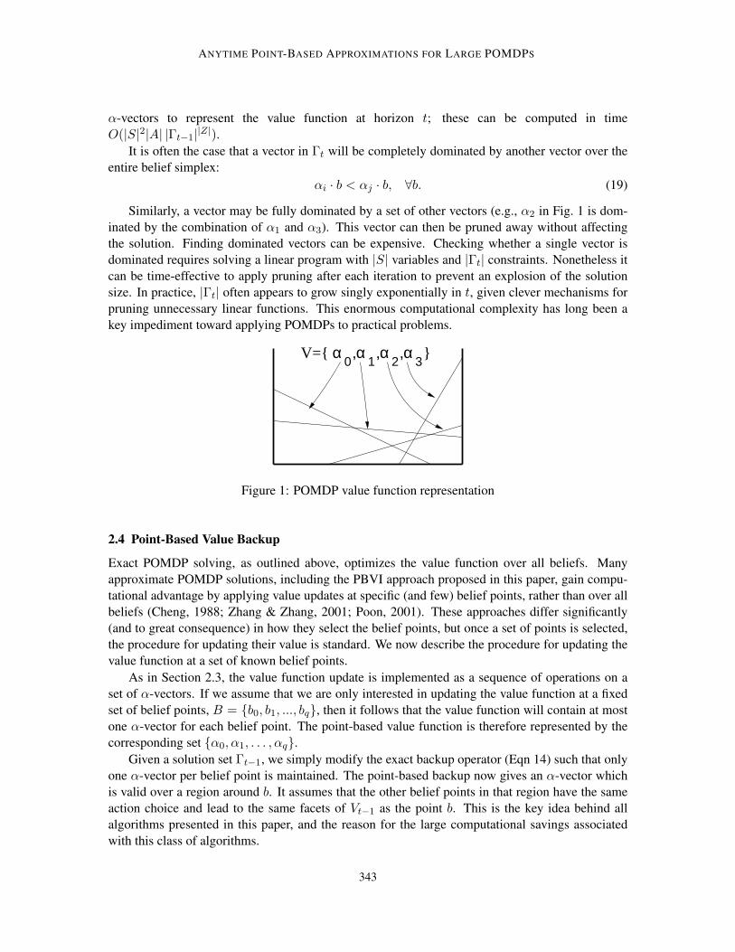
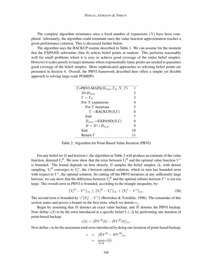
Similarly, a vector may be fully dominated by a set of other vectors (e.g., α2 in Fig. 1 is dom-inated by the combination of α1 and α3). This vector can then be pruned away without affectingthe solution. Finding dominated vectors can be expensive. Checking whether a single vector isdominated requires solving a linear program with |S| variables and |Γt| constraints. Nonetheless itcan be time-effective to apply pruning after each iteration to prevent an explosion of the solutionsize. In practice, |Γt| often appears to grow singly exponentially in t, given clever mechanisms forpruning unnecessary linear functions. This enormous computational complexity has long been akey impediment toward applying POMDPs to practical problems.
α 0V={ ,α 1,α 2,α 3}
Figure 1: POMDP value function representation
2.4 Point-Based Value Backup
Exact POMDP solving, as outlined above, optimizes the value function over all beliefs. Manyapproximate POMDP solutions, including the PBVI approach proposed in this paper, gain compu-tational advantage by applying value updates at specific (and few) belief points, rather than over allbeliefs (Cheng, 1988; Zhang & Zhang, 2001; Poon, 2001). These approaches differ significantly(and to great consequence) in how they select the belief points, but once a set of points is selected,the procedure for updating their value is standard. We now describe the procedure for updating thevalue function at a set of known belief points.
As in Section 2.3, the value function update is implemented as a sequence of operations on aset of α-vectors. If we assume that we are only interested in updating the value function at a fixedset of belief points, B = {b0, b1, ..., bq}, then it follows that the value function will contain at mostone α-vector for each belief point. The point-based value function is therefore represented by thecorresponding set {α0, α1, . . . , αq}.
Given a solution set Γt−1, we simply modify the exact backup operator (Eqn 14) such that onlyone α-vector per belief point is maintained. The point-based backup now gives an α-vector whichis valid over a region around b. It assumes that the other belief points in that region have the sameaction choice and lead to the same facets of Vt−1 as the point b. This is the key idea behind allalgorithms presented in this paper, and the reason for the large computational savings associatedwith this class of algorithms.
343
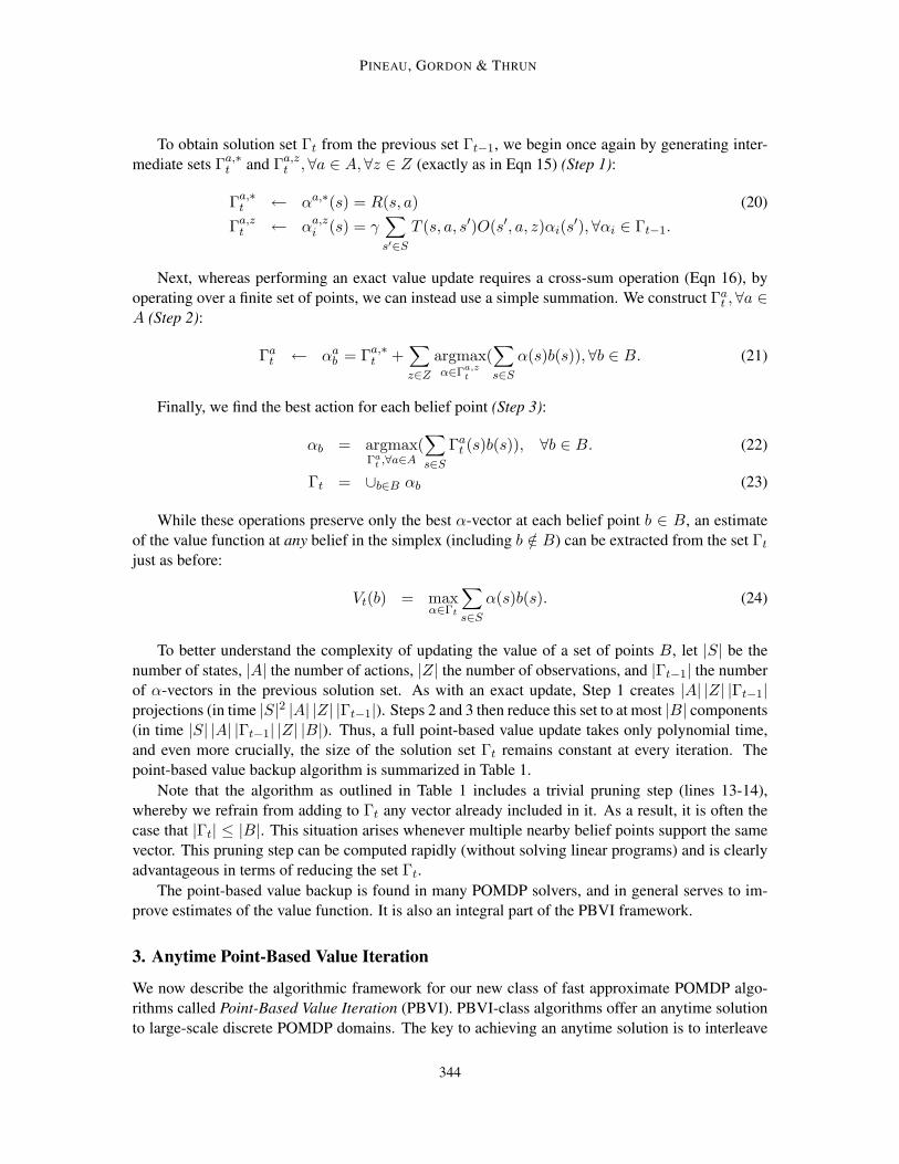
PINEAU, GORDON & THRUN
To obtain solution set Γt from the previous set Γt−1, we begin once again by generating inter-mediate sets Γa,∗
t and Γa,zt ,∀a ∈ A,∀z ∈ Z (exactly as in Eqn 15) (Step 1):
Γa,∗t ← αa,∗(s) = R(s, a) (20)
Γa,zt ← αa,z
i (s) = γ∑s′∈S
T (s, a, s′)O(s′, a, z)αi(s′),∀αi ∈ Γt−1.
Next, whereas performing an exact value update requires a cross-sum operation (Eqn 16), byoperating over a finite set of points, we can instead use a simple summation. We construct Γa
t ,∀a ∈A (Step 2):
Γat ← αa
b = Γa,∗t +
∑z∈Z
argmaxα∈Γa,z
t
(∑s∈S
α(s)b(s)),∀b ∈ B. (21)
Finally, we find the best action for each belief point (Step 3):
αb = argmaxΓa
t ,∀a∈A(∑s∈S
Γat (s)b(s)), ∀b ∈ B. (22)
Γt = ∪b∈B αb (23)
While these operations preserve only the best α-vector at each belief point b ∈ B, an estimateof the value function at any belief in the simplex (including b /∈ B) can be extracted from the set Γt
just as before:
Vt(b) = maxα∈Γt
∑s∈S
α(s)b(s). (24)
To better understand the complexity of updating the value of a set of points B, let |S| be thenumber of states, |A| the number of actions, |Z| the number of observations, and |Γt−1| the numberof α-vectors in the previous solution set. As with an exact update, Step 1 creates |A| |Z| |Γt−1|projections (in time |S|2 |A| |Z| |Γt−1|). Steps 2 and 3 then reduce this set to at most |B| components(in time |S| |A| |Γt−1| |Z| |B|). Thus, a full point-based value update takes only polynomial time,and even more crucially, the size of the solution set Γt remains constant at every iteration. Thepoint-based value backup algorithm is summarized in Table 1.
Note that the algorithm as outlined in Table 1 includes a trivial pruning step (lines 13-14),whereby we refrain from adding to Γt any vector already included in it. As a result, it is often thecase that |Γt| ≤ |B|. This situation arises whenever multiple nearby belief points support the samevector. This pruning step can be computed rapidly (without solving linear programs) and is clearlyadvantageous in terms of reducing the set Γt.
The point-based value backup is found in many POMDP solvers, and in general serves to im-prove estimates of the value function. It is also an integral part of the PBVI framework.
3. Anytime Point-Based Value Iteration
We now describe the algorithmic framework for our new class of fast approximate POMDP algo-rithms called Point-Based Value Iteration (PBVI). PBVI-class algorithms offer an anytime solutionto large-scale discrete POMDP domains. The key to achieving an anytime solution is to interleave
344
ANYTIME POINT-BASED APPROXIMATIONS FOR LARGE POMDPS
Γt=BACKUP(B, Γt−1) 1For each action a ∈ A 2
For each observation z ∈ Z 3For each solution vector αi ∈ Γt−1 4
αa,zi (s) = γ
∑s′∈S T (s, a, s′)O(s′, a, z)αi(s′),∀s ∈ S 5
End 6Γa,z
t = ∪i αa,zi 7
End 8End 9Γt = ∅ 10For each belief point b ∈ B 11
αb = argmaxa∈A
[∑s∈S R(s, a)b(s) +
∑z∈Z maxα∈Γa,z
t[∑
s∈S α(s)b(s)]]
12If(αb /∈ Γt) 13
Γt = Γt ∪ αb 14End 15Return Γt 16
Table 1: Point-based value backup
two main components: the point-based update described in Table 1 and steps of belief set selec-tion. The approximate value function we find is guaranteed to have bounded error (compared to theoptimal) for any discrete POMDP domain.
The current section focuses on the overall anytime algorithm and its theoretical properties, in-dependent of the belief point selection process. Section 4 then discusses in detail various noveltechniques for belief point selection.
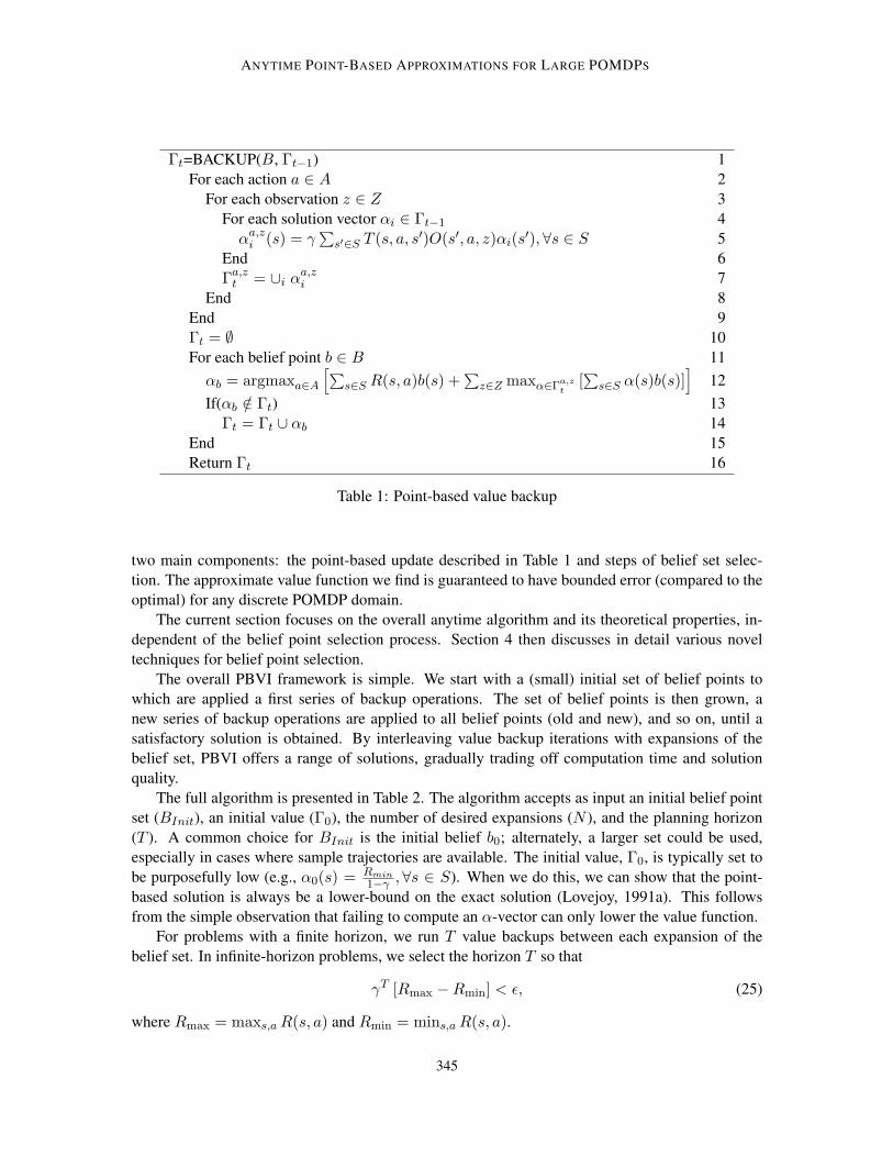
The overall PBVI framework is simple. We start with a (small) initial set of belief points towhich are applied a first series of backup operations. The set of belief points is then grown, anew series of backup operations are applied to all belief points (old and new), and so on, until asatisfactory solution is obtained. By interleaving value backup iterations with expansions of thebelief set, PBVI offers a range of solutions, gradually trading off computation time and solutionquality.
The full algorithm is presented in Table 2. The algorithm accepts as input an initial belief pointset (BInit), an initial value (Γ0), the number of desired expansions (N ), and the planning horizon(T ). A common choice for BInit is the initial belief b0; alternately, a larger set could be used,especially in cases where sample trajectories are available. The initial value, Γ0, is typically set tobe purposefully low (e.g., α0(s) = Rmin
1−γ ,∀s ∈ S). When we do this, we can show that the point-based solution is always be a lower-bound on the exact solution (Lovejoy, 1991a). This followsfrom the simple observation that failing to compute an α-vector can only lower the value function.
For problems with a finite horizon, we run T value backups between each expansion of thebelief set. In infinite-horizon problems, we select the horizon T so that
γT [Rmax −Rmin] < ε, (25)
where Rmax = maxs,a R(s, a) and Rmin = mins,a R(s, a).
345
PINEAU, GORDON & THRUN
The complete algorithm terminates once a fixed number of expansions (N ) have been com-pleted. Alternately, the algorithm could terminate once the value function approximation reaches agiven performance criterion. This is discussed further below.
The algorithm uses the BACKUP routine described in Table 1. We can assume for the momentthat the EXPAND subroutine (line 8) selects belief points at random. This performs reasonablywell for small problems where it is easy to achieve good coverage of the entire belief simplex.However it scales poorly to larger domains where exponentially many points are needed to guaranteegood coverage of the belief simplex. More sophisticated approaches to selecting belief points arepresented in Section 4. Overall, the PBVI framework described here offers a simple yet flexibleapproach to solving large-scale POMDPs.
Γ=PBVI-MAIN(BInit, Γ0, N , T ) 1B=BInit 2Γ = Γ0 3For N expansions 4
For T iterations 5Γ =BACKUP(B,Γ) 6
End 7Bnew =EXPAND(B,Γ) 8B = B ∪Bnew 9
End 10Return Γ 11
Table 2: Algorithm for Point-Based Value Iteration (PBVI)
For any belief set B and horizon t, the algorithm in Table 2 will produce an estimate of the valuefunction, denoted V B
t . We now show that the error between V Bt and the optimal value function V ∗
is bounded. The bound depends on how densely B samples the belief simplex ∆; with densersampling, V B
t converges to V ∗t , the t-horizon optimal solution, which in turn has bounded error
with respect to V ∗, the optimal solution. So cutting off the PBVI iterations at any sufficiently largehorizon, we can show that the difference between V B
t and the optimal infinite-horizon V ∗ is not toolarge. The overall error in PBVI is bounded, according to the triangle inequality, by:
‖V Bt − V ∗‖∞ ≤ ‖V B
t − V ∗t ‖∞ + ‖V ∗
t − V ∗‖∞. (26)
The second term is bounded by γt‖V ∗0 − V ∗‖ (Bertsekas & Tsitsiklis, 1996). The remainder of this
section states and proves a bound on the first term, which we denote εt.Begin by assuming that H denotes an exact value backup, and H denotes the PBVI backup.
Now define ε(b) to be the error introduced at a specific belief b ∈ ∆ by performing one iteration ofpoint-based backup:
ε(b) = |HV B(b)−HV B(b)|∞.
Next define ε to be the maximum total error introduced by doing one iteration of point-based backup:
ε = |HV B −HV B|∞= max
b∈∆ε(b).
346

ANYTIME POINT-BASED APPROXIMATIONS FOR LARGE POMDPS
Finally define the density δB of a set of belief points B to be the maximum distance from any beliefin the simplex ∆ to a belief in set B. More precisely:
δB = maxb′∈∆
minb∈B‖b− b′‖1. (27)
Now we can prove the following lemma:
Lemma 1. The error introduced in PBVI when performing one iteration of value backup over B,instead of over ∆, is bounded by
ε ≤ (Rmax −Rmin)δB
1− γ
Proof: Let b′ ∈ ∆ be the point where PBVI makes its worst error in value update, and b ∈ Bbe the closest (1-norm) sampled belief to b′. Let α be the vector that is maximal at b, and α′ be thevector that would be maximal at b′. By failing to include α′ in its solution set, PBVI makes an errorof at most α′ · b′ − α · b′. On the other hand, since α is maximal at b, then α′ · b ≤ α · b. So,
ε ≤ α′ · b′ − α · b′
= α′ · b′ − α · b′ + (α′ · b− α′ · b) Add zero≤ α′ · b′ − α · b′ + α · b− α′ · b Assume α is optimal at b
= (α′ − α) · (b′ − b) Re-arrange the terms≤ ‖α′ − α‖∞‖b′ − b‖1 By Holder inequality≤ ‖α′ − α‖∞δB By definition of δB
≤ (Rmax−Rmin)δB
1−γ
The last inequality holds because each α-vector represents the reward achievable starting fromsome state and following some sequence of actions and observations. Therefore the sum of rewardsmust fall between Rmin
1−γ and Rmax1−γ .
Lemma 1 states a bound on the approximation error introduced by one iteration of point-basedvalue updates within the PBVI framework. We now look at the bound over multiple value updates.
Theorem 3.1. For any belief set B and any horizon t, the error of the PBVI algorithm εt = ‖V Bt −
V ∗t ‖∞ is bounded by
εt ≤(Rmax −Rmin)δB
(1− γ)2
Proof:
εt = ||V Bt − V ∗
t ||∞= ||HV B
t−1 −HV ∗t−1||∞ By definition of H
≤ ||HV Bt−1 −HV B
t−1||∞ + ||HV Bt−1 −HV ∗
t−1||∞ By triangle inequality
≤ (Rmax−Rmin)δB
1−γ + ||HV Bt−1 −HV ∗
t−1||∞ By lemma 1
≤ (Rmax−Rmin)δB
1−γ + γ||V Bt−1 − V ∗
t−1||∞ By contraction of exact value backup
= (Rmax−Rmin)δB
1−γ + γεt−1 By definition of εt−1
≤ (Rmax−Rmin)δB
(1−γ)2By sum of a geometric series
347

PINEAU, GORDON & THRUN
The bound described in this section depends on how densely B samples the belief simplex ∆.In the case where not all beliefs are reachable, PBVI does not need to sample all of ∆ densely, butcan replace ∆ by the set of reachable beliefs ∆ (Fig. 2). The error bounds and convergence resultshold on ∆. We simply need to re-define b′ ∈ ∆ in lemma 1.
As a side note, it is worth pointing out that because PBVI makes no assumption regardingthe initial value function V B
0 , the point-based solution V B is not guaranteed to improve with theaddition of belief points. Nonetheless, the theorem presented in this section shows that the boundon the error between V B
t (the point-based solution) and V ∗ (the optimal solution) is guaranteedto decrease (or stay the same) with the addition of belief points. In cases where V B
t is initializedpessimistically (e.g., V B
0 (s) = Rmin1−γ ,∀s ∈ S, as suggested above), then V B
t will improve (or staythe same) with each value backup and addition of belief points.
This section has thus far skirted the issue of belief point selection, however the bound presentedin this section clearly argues in favor of dense sampling over the belief simplex. While randomlyselecting points according to a uniform distribution may eventually accomplish this, it is generallyinefficient, in particular for high dimensional cases. Furthermore, it does not take advantage ofthe fact that the error bound holds for dense sampling over reachable beliefs. Thus we seek moreefficient ways to generate belief points than at random over the entire simplex. This is the issueexplored in the next section.
4. Belief Point Selection
In section 3, we outlined the prototypical PBVI algorithm, while conveniently avoiding the questionof how and when belief points should be selected. There is a clear trade-off between including fewerbeliefs (which would favor fast planning over good performance), versus including many beliefs(which would slow down planning, but ensure a better bound on performance). This brings up thequestion of how many belief points should be included. However the number of points is not the onlyconsideration. It is likely that some collections of belief points (e.g., those frequently encountered)are more likely to produce a good value function than others. This brings up the question of whichbeliefs should be included.
A number of approaches have been proposed in the literature. For example, some exact valuefunction approaches use linear programs to identify points where the value function needs to befurther improved (Cheng, 1988; Littman, 1996; Zhang & Zhang, 2001), however this is typicallyvery expensive. The value function can also be approximated by learning the value at regular points,using a fixed-resolution (Lovejoy, 1991a), or variable-resolution (Zhou & Hansen, 2001) grid. Thisis less expensive than solving LPs, but can scales poorly as the number of states increases. Alter-nately, one can use heuristics to generate grid-points (Hauskrecht, 2000; Poon, 2001). This tendsto be more scalable, though significant experimentation is required to establish which heuristics aremost useful.
This section presents five heuristic strategies for selecting belief points, from fast and naiverandom sampling, to increasingly more sophisticated stochastic simulation techniques. The mosteffective strategy we propose is one that carefully selects points that are likely to have the largestimpact in reducing the error bound (Theorem 3.1).
Most of the strategies we consider focus on selecting reachable beliefs, rather than gettinguniform coverage over the entire belief simplex. Therefore it is useful to begin this discussion bylooking at how reachability is assessed.
348
ANYTIME POINT-BASED APPROXIMATIONS FOR LARGE POMDPS
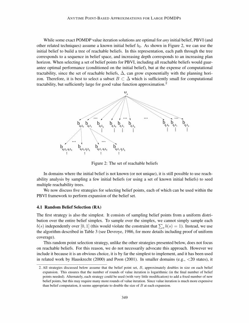
While some exact POMDP value iteration solutions are optimal for any initial belief, PBVI (andother related techniques) assume a known initial belief b0. As shown in Figure 2, we can use theinitial belief to build a tree of reachable beliefs. In this representation, each path through the treecorresponds to a sequence in belief space, and increasing depth corresponds to an increasing planhorizon. When selecting a set of belief points for PBVI, including all reachable beliefs would guar-antee optimal performance (conditioned on the initial belief), but at the expense of computationaltractability, since the set of reachable beliefs, ∆, can grow exponentially with the planning hori-zon. Therefore, it is best to select a subset B ⊂ ∆ which is sufficiently small for computationaltractability, but sufficiently large for good value function approximation.2
b1 0a z b
1 1a z b1 qa z
bp 0a z b
p 1a z bp qa z
b0
b0 0 0 0a z a z
b0 0 p qa z a z b
0 1 0 0a z a z b0 1 p qa z a z
b0 0a z b
0 1a z b0 qa z
... ... ...
... ...
... ... ... ...
... ... ......
... ... ...
...
Figure 2: The set of reachable beliefs
In domains where the initial belief is not known (or not unique), it is still possible to use reach-ability analysis by sampling a few initial beliefs (or using a set of known initial beliefs) to seedmultiple reachability trees.
We now discuss five strategies for selecting belief points, each of which can be used within thePBVI framework to perform expansion of the belief set.
4.1 Random Belief Selection (RA)
The first strategy is also the simplest. It consists of sampling belief points from a uniform distri-bution over the entire belief simplex. To sample over the simplex, we cannot simply sample eachb(s) independently over [0, 1] (this would violate the constraint that
∑s b(s) = 1). Instead, we use
the algorithm described in Table 3 (see Devroye, 1986, for more details including proof of uniformcoverage).
This random point selection strategy, unlike the other strategies presented below, does not focuson reachable beliefs. For this reason, we do not necessarily advocate this approach. However weinclude it because it is an obvious choice, it is by far the simplest to implement, and it has been usedin related work by Hauskrecht (2000) and Poon (2001). In smaller domains (e.g., <20 states), it
2. All strategies discussed below assume that the belief point set, B, approximately doubles in size on each beliefexpansion. This ensures that the number of rounds of value iteration is logarithmic (in the final number of beliefpoints needed). Alternately, each strategy could be used (with very little modification) to add a fixed number of newbelief points, but this may require many more rounds of value iteration. Since value iteration is much more expensivethan belief computation, it seems appropriate to double the size of B at each expansion.
349
PINEAU, GORDON & THRUN
Bnew=EXPANDRA(B, Γ) 1Bnew= B 2Foreach b ∈ B 3
S := number of states 4For i = 0 : S 5
btmp[i]=randuniform(0,1) 6End 7Sort btmp in ascending order 8For i = 1 : S − 1 9
bnew[i]=btmp[i + 1]− btmp[i] 10End 11Bnew = Bnew ∪ bnew 12
End 13Return Bnew 14
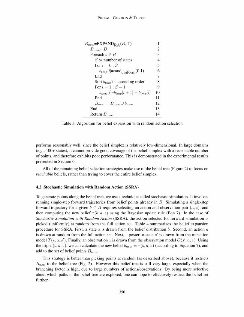
Table 3: Algorithm for belief expansion with random action selection
performs reasonably well, since the belief simplex is relatively low-dimensional. In large domains(e.g., 100+ states), it cannot provide good coverage of the belief simplex with a reasonable numberof points, and therefore exhibits poor performance. This is demonstrated in the experimental resultspresented in Section 6.
All of the remaining belief selection strategies make use of the belief tree (Figure 2) to focus onreachable beliefs, rather than trying to cover the entire belief simplex.
4.2 Stochastic Simulation with Random Action (SSRA)
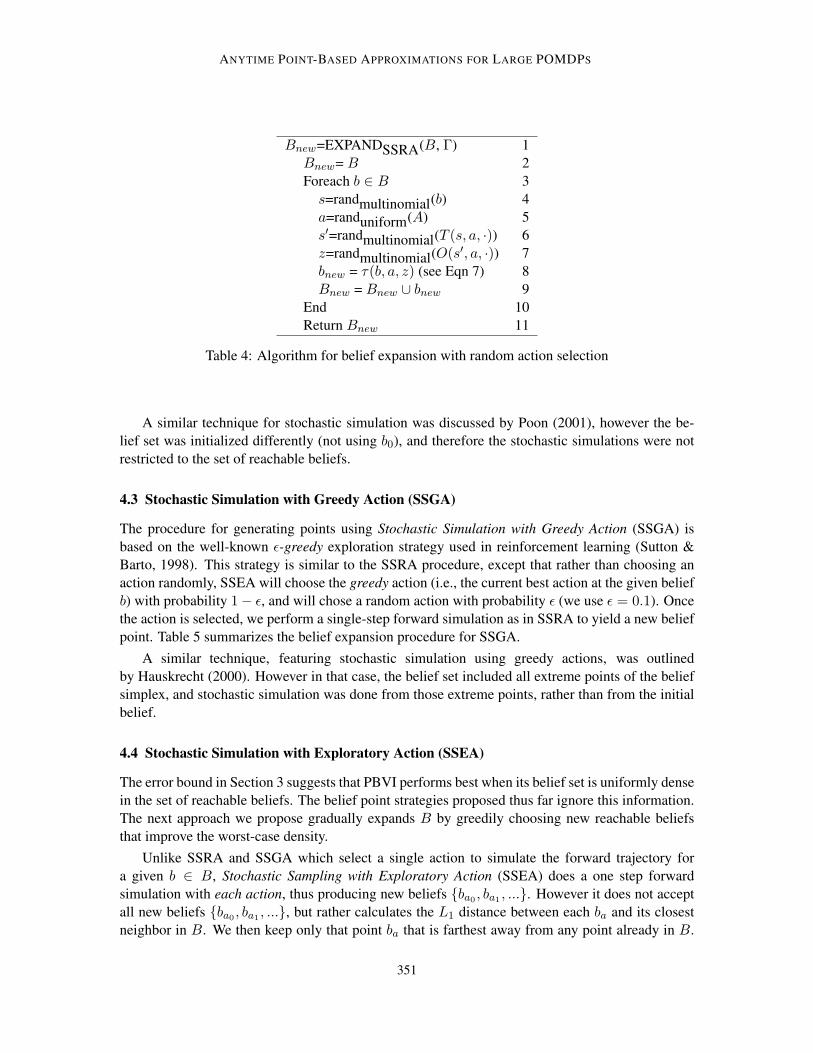
To generate points along the belief tree, we use a technique called stochastic simulation. It involvesrunning single-step forward trajectories from belief points already in B. Simulating a single-stepforward trajectory for a given b ∈ B requires selecting an action and observation pair (a, z), andthen computing the new belief τ(b, a, z) using the Bayesian update rule (Eqn 7). In the case ofStochastic Simulation with Random Action (SSRA), the action selected for forward simulation ispicked (uniformly) at random from the full action set. Table 4 summarizes the belief expansionprocedure for SSRA. First, a state s is drawn from the belief distribution b. Second, an action ais drawn at random from the full action set. Next, a posterior state s′ is drawn from the transitionmodel T (s, a, s′). Finally, an observation z is drawn from the observation model O(s′, a, z). Usingthe triple (b, a, z), we can calculate the new belief bnew = τ(b, a, z) (according to Equation 7), andadd to the set of belief points Bnew.
This strategy is better than picking points at random (as described above), because it restrictsBnew to the belief tree (Fig. 2). However this belief tree is still very large, especially when thebranching factor is high, due to large numbers of actions/observations. By being more selectiveabout which paths in the belief tree are explored, one can hope to effectively restrict the belief setfurther.
350
ANYTIME POINT-BASED APPROXIMATIONS FOR LARGE POMDPS
Bnew=EXPANDSSRA(B, Γ) 1Bnew= B 2Foreach b ∈ B 3
s=randmultinomial(b) 4a=randuniform(A) 5s′=randmultinomial(T (s, a, ·)) 6z=randmultinomial(O(s′, a, ·)) 7bnew = τ(b, a, z) (see Eqn 7) 8Bnew = Bnew ∪ bnew 9
End 10Return Bnew 11
Table 4: Algorithm for belief expansion with random action selection
A similar technique for stochastic simulation was discussed by Poon (2001), however the be-lief set was initialized differently (not using b0), and therefore the stochastic simulations were notrestricted to the set of reachable beliefs.
4.3 Stochastic Simulation with Greedy Action (SSGA)
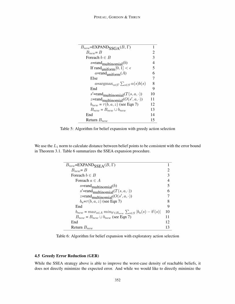
The procedure for generating points using Stochastic Simulation with Greedy Action (SSGA) isbased on the well-known ε-greedy exploration strategy used in reinforcement learning (Sutton &Barto, 1998). This strategy is similar to the SSRA procedure, except that rather than choosing anaction randomly, SSEA will choose the greedy action (i.e., the current best action at the given beliefb) with probability 1− ε, and will chose a random action with probability ε (we use ε = 0.1). Oncethe action is selected, we perform a single-step forward simulation as in SSRA to yield a new beliefpoint. Table 5 summarizes the belief expansion procedure for SSGA.
A similar technique, featuring stochastic simulation using greedy actions, was outlinedby Hauskrecht (2000). However in that case, the belief set included all extreme points of the beliefsimplex, and stochastic simulation was done from those extreme points, rather than from the initialbelief.
4.4 Stochastic Simulation with Exploratory Action (SSEA)
The error bound in Section 3 suggests that PBVI performs best when its belief set is uniformly densein the set of reachable beliefs. The belief point strategies proposed thus far ignore this information.The next approach we propose gradually expands B by greedily choosing new reachable beliefsthat improve the worst-case density.
Unlike SSRA and SSGA which select a single action to simulate the forward trajectory fora given b ∈ B, Stochastic Sampling with Exploratory Action (SSEA) does a one step forwardsimulation with each action, thus producing new beliefs {ba0 , ba1 , ...}. However it does not acceptall new beliefs {ba0 , ba1 , ...}, but rather calculates the L1 distance between each ba and its closestneighbor in B. We then keep only that point ba that is farthest away from any point already in B.
351
PINEAU, GORDON & THRUN
Bnew=EXPANDSSGA(B, Γ) 1Bnew= B 2Foreach b ∈ B 3
s=randmultinomial(b) 4If randuniform[0, 1] < ε 5
a=randuniform(A) 6Else 7
a=argmaxα∈Γ
∑s∈S α(s)b(s) 8
End 9s′=randmultinomial(T (s, a, ·)) 10z=randmultinomial(O(s′, a, ·)) 11bnew = τ(b, a, z) (see Eqn 7) 12Bnew = Bnew ∪ bnew 13
End 14Return Bnew 15
Table 5: Algorithm for belief expansion with greedy action selection
We use the L1 norm to calculate distance between belief points to be consistent with the error boundin Theorem 3.1. Table 6 summarizes the SSEA expansion procedure.
Bnew=EXPANDSSEA(B, Γ) 1Bnew= B 2Foreach b ∈ B 3
Foreach a ∈ A 4s=randmultinomial(b) 5s′=randmultinomial(T (s, a, ·)) 6z=randmultinomial(O(s′, a, ·)) 7ba=τ(b, a, z) (see Eqn 7) 8
End 9bnew = maxa∈A minb′∈Bnew
∑s∈S |ba(s)− b′(s)| 10
Bnew = Bnew ∪ bnew (see Eqn 7) 11End 12Return Bnew 13
Table 6: Algorithm for belief expansion with exploratory action selection
4.5 Greedy Error Reduction (GER)
While the SSEA strategy above is able to improve the worst-case density of reachable beliefs, itdoes not directly minimize the expected error. And while we would like to directly minimize the
352
ANYTIME POINT-BASED APPROXIMATIONS FOR LARGE POMDPS
error, all we can measure is a bound on the error (Lemma 1). We therefore propose a final strategywhich greedily adds the candidate beliefs that will most effectively reduce this error bound. Ourempirical results, as presented below, show that this strategy is the most successful one discoveredthus far.
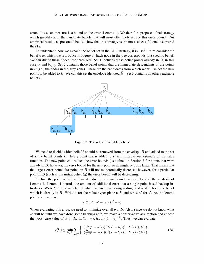
To understand how we expand the belief set in the GER strategy, it is useful to re-consider thebelief tree, which we reproduce in Figure 3. Each node in the tree corresponds to a specific belief.We can divide these nodes into three sets. Set 1 includes those belief points already in B, in thiscase b0 and ba0z0 . Set 2 contains those belief points that are immediate descendants of the pointsin B (i.e., the nodes in the grey zone). These are the candidates from which we will select the newpoints to be added to B. We call this set the envelope (denoted B). Set 3 contains all other reachablebeliefs.
b1 0a z b
1 1a z b1 qa z
bp 0a z b
p 1a z bp qa z
b0
b0 0 0 0a z a z
b0 0 p qa z a z
b0 0a z b
0 1a z b0 qa z... ... ......
... ... ......
... ...
... ... ...
...
...
Figure 3: The set of reachable beliefs
We need to decide which belief b should be removed from the envelope B and added to the setof active belief points B. Every point that is added to B will improve our estimate of the valuefunction. The new point will reduce the error bounds (as defined in Section 3 for points that werealready in B; however, the error bound for the new point itself might be quite large. That means thatthe largest error bound for points in B will not monotonically decrease; however, for a particularpoint in B (such as the initial belief b0) the error bound will be decreasing.
To find the point which will most reduce our error bound, we can look at the analysis ofLemma 1. Lemma 1 bounds the amount of additional error that a single point-based backup in-troduces. Write b′ for the new belief which we are considering adding, and write b for some beliefwhich is already in B. Write α for the value hyper-plane at b, and write α′ for b′. As the lemmapoints out, we have
ε(b′) ≤ (α′ − α) · (b′ − b)
When evaluating this error, we need to minimize over all b ∈ B. Also, since we do not know whatα′ will be until we have done some backups at b′, we make a conservative assumption and choosethe worst-case value of α′ ∈ [Rmin/(1− γ), Rmax/(1− γ)]|S|. Thus, we can evaluate:
ε(b′) ≤ minb∈B
∑s∈S
{(Rmax
1−γ − α(s))(b′(s)− b(s)) b′(s) ≥ b(s)(Rmin
1−γ − α(s))(b′(s)− b(s)) b′(s) < b(s)(28)
353
PINEAU, GORDON & THRUN
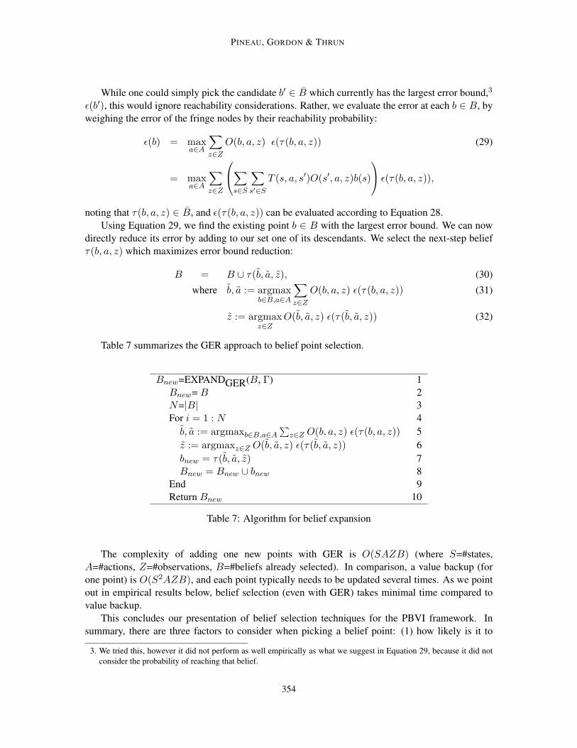
While one could simply pick the candidate b′ ∈ B which currently has the largest error bound,3
ε(b′), this would ignore reachability considerations. Rather, we evaluate the error at each b ∈ B, byweighing the error of the fringe nodes by their reachability probability:
ε(b) = maxa∈A
∑z∈Z
O(b, a, z) ε(τ(b, a, z)) (29)
= maxa∈A
∑z∈Z
∑s∈S
∑s′∈S
T (s, a, s′)O(s′, a, z)b(s)
ε(τ(b, a, z)),
noting that τ(b, a, z) ∈ B, and ε(τ(b, a, z)) can be evaluated according to Equation 28.Using Equation 29, we find the existing point b ∈ B with the largest error bound. We can now
directly reduce its error by adding to our set one of its descendants. We select the next-step beliefτ(b, a, z) which maximizes error bound reduction:
B = B ∪ τ(b, a, z), (30)
where b, a := argmaxb∈B,a∈A
∑z∈Z
O(b, a, z) ε(τ(b, a, z)) (31)
z := argmaxz∈Z
O(b, a, z) ε(τ(b, a, z)) (32)
Table 7 summarizes the GER approach to belief point selection.
Bnew=EXPANDGER(B, Γ) 1Bnew= B 2N=|B| 3For i = 1 : N 4
b, a := argmaxb∈B,a∈A
∑z∈Z O(b, a, z) ε(τ(b, a, z)) 5
z := argmaxz∈Z O(b, a, z) ε(τ(b, a, z)) 6bnew = τ(b, a, z) 7Bnew = Bnew ∪ bnew 8
End 9Return Bnew 10
Table 7: Algorithm for belief expansion
The complexity of adding one new points with GER is O(SAZB) (where S=#states,A=#actions, Z=#observations, B=#beliefs already selected). In comparison, a value backup (forone point) is O(S2AZB), and each point typically needs to be updated several times. As we pointout in empirical results below, belief selection (even with GER) takes minimal time compared tovalue backup.
This concludes our presentation of belief selection techniques for the PBVI framework. Insummary, there are three factors to consider when picking a belief point: (1) how likely is it to
3. We tried this, however it did not perform as well empirically as what we suggest in Equation 29, because it did notconsider the probability of reaching that belief.
354
ANYTIME POINT-BASED APPROXIMATIONS FOR LARGE POMDPS
occur? (2) how far is it from other belief points already selected? (3) what is the current approximatevalue for that point? The simplest heuristic (RA) accounts for none of these, whereas some of theothers (SSRA, SSGA, SSEA) account for one, and GER incorporates all three factors.
4.6 Belief Expansion Example
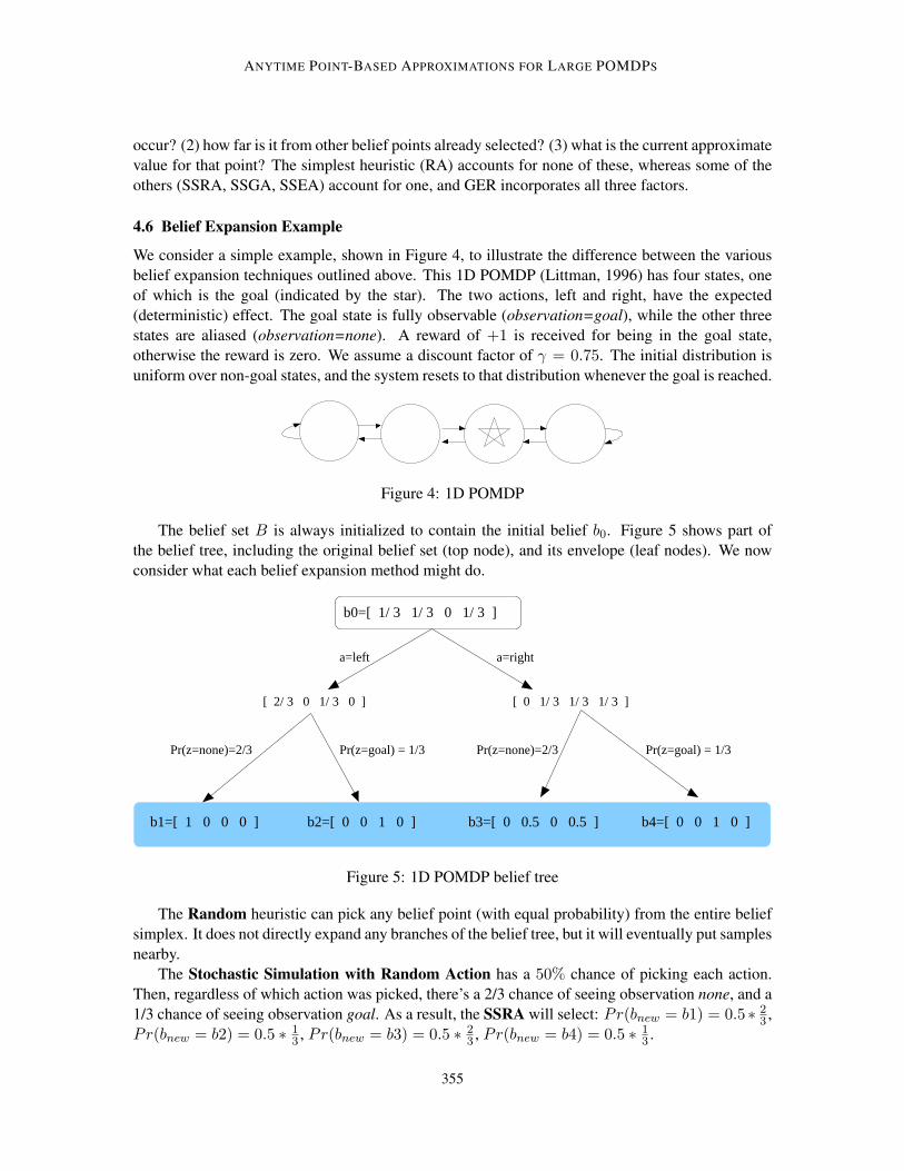
We consider a simple example, shown in Figure 4, to illustrate the difference between the variousbelief expansion techniques outlined above. This 1D POMDP (Littman, 1996) has four states, oneof which is the goal (indicated by the star). The two actions, left and right, have the expected(deterministic) effect. The goal state is fully observable (observation=goal), while the other threestates are aliased (observation=none). A reward of +1 is received for being in the goal state,otherwise the reward is zero. We assume a discount factor of γ = 0.75. The initial distribution isuniform over non-goal states, and the system resets to that distribution whenever the goal is reached.
Figure 4: 1D POMDP
The belief set B is always initialized to contain the initial belief b0. Figure 5 shows part ofthe belief tree, including the original belief set (top node), and its envelope (leaf nodes). We nowconsider what each belief expansion method might do.
b2=[ 0 0 1 0 ] b4=[ 0 0 1 0 ]b3=[ 0 0.5 0 0.5 ]b1=[ 1 0 0 0 ]
b0=[ 1/ 3 1/ 3 0 1/ 3 ]
a=righta=left
[ 2/ 3 0 1/ 3 0 ] [ 0 1/ 3 1/ 3 1/ 3 ]
Pr(z=none)=2/3 Pr(z=none)=2/3 Pr(z=goal) = 1/3Pr(z=goal) = 1/3
Figure 5: 1D POMDP belief tree
The Random heuristic can pick any belief point (with equal probability) from the entire beliefsimplex. It does not directly expand any branches of the belief tree, but it will eventually put samplesnearby.
The Stochastic Simulation with Random Action has a 50% chance of picking each action.Then, regardless of which action was picked, there’s a 2/3 chance of seeing observation none, and a1/3 chance of seeing observation goal. As a result, the SSRA will select: Pr(bnew = b1) = 0.5∗ 2
3 ,Pr(bnew = b2) = 0.5 ∗ 1
3 , Pr(bnew = b3) = 0.5 ∗ 23 , Pr(bnew = b4) = 0.5 ∗ 1
3 .
355

PINEAU, GORDON & THRUN
The Stochastic Simulation with Greedy Action first needs to know the policy at b0. A fewiterations of point-based updates (Section 2.4) applied to this initial (single point) belief set revealthat π(b0) = left.4 As a result, expansion of the belief will greedily select action left with proba-bility 1− ε + ε
|A| = 0.95 (assuming ε = 0.1 and |A| = 2). Action right will be selected for beliefexpansion with probability ε
|A| = 0.05. Combining this along with the observation probabilities, wecan tell that SSGA will expand as follows: Pr(bnew = b1) = 0.95 ∗ 2
3 , Pr(bnew = b2) = 0.95 ∗ 13 ,
Pr(bnew = b3) = 0.05 ∗ 23 , Pr(bnew = b4) = 0.05 ∗ 1
3 .Predicting the choice of Stochastic Simulation with Exploratory Action is slightly more com-
plicated. Four cases can occur, depending on the outcomes of random forward simulation from b0:
1. If action left goes to b1 (Pr = 2/3) and action right goes to b3 (Pr = 2/3), then b1 will beselected because ||b0 − b1||1 = 4/3 whereas ||b0 − b3||1 = 2/3. This case will occur withPr = 4/9.
2. If action left goes to b1 (Pr = 2/3) and action right goes to b4 (Pr = 1/3), then b4 will beselected because ||b0 − b4||1 = 2. This case will occur with Pr = 2/9.
3. If action left goes to b2 (Pr = 1/3) and action right goes to b3 (Pr = 2/3), then b2 will beselected because ||b0 − b2||1 = 2. This case will occur with Pr = 2/9.
4. If action left goes to b2 (Pr = 1/3) and action right goes to b4 (Pr = 1/3), then either canbe selected (since they are equidistant to b0). In this case each b2 and b4 has Pr = 1/18 ofbeing selected.
All told, Pr(bnew = b1) = 4/9, Pr(bnew = b2) = 5/18, Pr(bnew = b3) = 0, Pr(bnew = b4) =5/18.
Now looking at belief expansion using Greedy Error Reduction, we need to compute theerror ε(τ(b0, a, z)),∀a, z. We consider Equation 28: since B has only one point, b0, then nec-essarily b = b0. To estimate α, we apply multiple steps of value backup at b0 and obtainα = [0.94 0.94 0.92 1.74]. Using b and α as such, we can now estimate the error at each can-didate belief: ε(b1) = 2.93, ε(b2) = 4.28, ε(b3) = 1.20, ε(b4) = 4.28. Note that because B hasonly one point, the dominating factor is their distance to b0. Next, we factor in the observationprobabilities, as in Eqns 31-32, which allows us to determine that a = left and z = none, andtherefore we should select bnew = b1.
In summary, we note that SSGA, SSEA and GER all favor selecting b1, whereas SSRA pickseach option with equal probability (considering that b2 and b4 are actually the same). In general,for a problem of this size, it is reasonable to expand the entire belief tree. Any of the techniquesdiscussed here will be do this quickly, except RA which will not pick the exact nodes in the belieftree, but will select equally good nearby beliefs. This example is provided simply to illustrate thedifferent choices made by each strategy.
5. A Review of Point-Based Approaches for POMDP Solving
The previous section describes a new class of point-based algorithms for POMDP solving. The ideaof using point-based updates in POMDPs has been explored previously in the literature, and in this
4. This may not be obvious to the reader, but it follows directly from the repeated application of equations 20–23.
356
ANYTIME POINT-BASED APPROXIMATIONS FOR LARGE POMDPS
section we summarize the main results. For most of the approaches discussed below, the procedurefor updating the value function at a given point remains unchanged (as outlined in Section 2.4).Rather, the approaches are mainly differentiated by how the belief points are selected, and by howthe updates are ordered.
5.1 Exact Point-Based Algorithms
Some of the earlier exact POMDP techniques use point-based backups to optimize the value func-tion over limited regions of the belief simplex (Sondik, 1971; Cheng, 1988). These techniquestypically require solving multiple linear programs to find candidate belief points where the valuefunction is sub-optimal, which can be an expensive operation. Furthermore, to guarantee that an ex-act solution is found, relevant beliefs must be generated systematically, meaning that all reachablebeliefs must be considered. As a result, these methods typically cannot scale beyond a handful ofstates/actions/observations.
In work by Zhang and Zhang (2001), point-based updates are interleaved with standard dy-namic programming updates to further accelerate planning. In this case the points are not generatedsystematically, but rather backups are applied to both a set of witness points and LP points. Thewitness points are identified as a result of the standard dynamic programming updates, whereasthe LP points are identified by solving linear programs to identify beliefs where the value has notyet been improved. Both of these procedures are significantly more expensive than the belief se-lection heuristics presented in this paper and results are limited to domains with at most a dozenstates/actions/observations. Nonetheless this approach is guaranteed to converge to the optimal so-lution.
5.2 Grid-Based Approximations
There exists many approaches that approximate the value function using a finite set of belief pointsalong with their values. These points are often distributed according to a grid pattern over the beliefspace, thus the name grid-based approximation. An interpolation-extrapolation rule specifies thevalue at non-grid points as a function of the value of neighboring grid-points. These approachesignore the convexity of the POMDP value function.
Performing value backups over grid-points is relatively straightforward: dynamic programmingupdates as specified in Equation 11 can be adapted to grid-points for a simple polynomial-timealgorithm. Given a set of grid points G, the value at each bG ∈ G is defined by:
V (bG) = maxa
[∑s∈S
bG(s)R(s, a) + γ∑z∈Z
Pr(z | a, b)V (τ(b, a, z))
]. (33)
If τ(b, a, z) is part of the grid, then V (τ(b, a, z)) is defined by the value backups. Otherwise,V (τ(b, a, z)) is approximated using an interpolation rule such as:
V (τ(b, a, z) =|G|∑i=1
λ(i)V (bGi ), (34)
where λ(i) ≥ 0 and∑|G|
i=1 λ(i) = 1. This produces a convex combination over grid-points. Thetwo more interesting questions with respect to grid-based approximations are (1) how to calculatethe interpolation function; and (2) how to select grid points.
357
PINEAU, GORDON & THRUN
In general, to find the interpolation that leads to the best value function approximation at a pointb requires solving the following linear program:
Minimize|G|∑i=1
λ(i)V (bGi ) (35)
Subject to b =|G|∑i=1
λ(i)bGi (36)
|G|∑i=1
λ(i) = 1 (37)
0 ≤ λ(i) ≤ 1, 1 ≤ i ≤ |G|. (38)
Different approaches have been proposed to select grid points. Lovejoy (1991a) constructs afixed-resolution regular grid over the entire belief space. A benefit is that value interpolations can becalculated quickly by considering only neighboring grid-points. The disadvantage is that the numberof grid points grows exponentially with the dimensionality of the belief (i.e., with the number ofstates). A simpler approach would be to select random points over the belief space (Hauskrecht,1997). But this requires slower interpolation for estimating the value of the new points. Bothof these methods are less than ideal when the beliefs encountered are not uniformly distributed.In particular, many problems are characterized by dense beliefs at the edges of the simplex (i.e.,probability mass focused on a few states, and most other states have zero probability), and lowbelief density in the middle of the simplex. A distribution of grid-points that better reflects theactual distribution over belief points is therefore preferable.
Alternately, Hauskrecht (1997) also proposes using the corner points of the belief simplex (e.g.,[1 0 0 . . . ], [0 1 0 . . . ], . . . , [0 0 0 . . . 1]), and generating additional successor belief points throughone-step stochastic simulations (Eqn 7) from the corner points. He also proposes an approximateinterpolation algorithm that uses the values at |S|−1 critical points plus one non-critical point in thegrid. An alternative approach is that by Brafman (1997), which builds a grid by also starting with thecritical points of the belief simplex, but then uses a heuristic to estimate the usefulness of graduallyadding intermediate points (e.g., bk = 0.5bi + 0.5bj , for any pair of points). Both Hauskrecht’sand Brafman’s methods—generally referred to as non-regular grid approximations—require fewerpoints than Lovejoy’s regular grid approach. However the interpolation rule used to calculate thevalue at non-grid points is typically more expensive to compute, since it involves searching over allgrid points, rather than just the neighboring sub-simplex.
Zhou and Hansen (2001) propose a grid-based approximation that combines advantages fromboth regular and non-regular grids. The idea is to sub-sample the regular fixed-resolution gridproposed by Lovejoy. This gives a variable resolution grid since some parts of the beliefs can bemore densely sampled than others and by restricting grid points to lie on the fixed-resolution gridthe approach can guarantee fast value interpolation for non-grid points. Nonetheless, the algorithmoften requires a large number of grid points to achieve good performance.
Finally, Bonet (2002) proposes the first grid-based algorithm for POMDPs with ε-optimality(for any ε > 0). This approach requires thorough coverage of the belief space such that every pointis within δ of a grid-point. The value update for each grid point is fast to implement, since theinterpolation rule depends only on the nearest neighbor of the one-step successor belief for eachgrid point (which can be pre-computed). The main limitation is the fact that ε-coverage of the belief
358
ANYTIME POINT-BASED APPROXIMATIONS FOR LARGE POMDPS
space can only be attained by using exponentially many grid points. Furthermore, this methodrequires good coverage of the entire belief space, as opposed to the algorithms of Section 4, whichfocus on coverage of the reachable beliefs.
5.3 Approximate Point-Based Algorithms
More similar to the PBVI-class of algorithms are those approaches that update both the value andgradient at each grid point (Lovejoy, 1991a; Hauskrecht, 2000; Poon, 2001). These methods are ableto preserve the piecewise linearity and convexity of the value function, and define a value functionover the entire belief simplex. Most of these methods use random beliefs, and/or require the inclu-sion of a large number of fixed beliefs such as the corners of the probability simplex. In contrast, thePBVI-class algorithms we propose (with the exception of PBVI+RA) select only reachable beliefs,and in particular those belief points that improve the error bounds as quickly as possible. The ideaof using reachability analysis (also known as stochastic simulation) to generate new points was ex-plored by some of the earlier approaches (Hauskrecht, 2000; Poon, 2001). However their analysisindicated that stochastic simulation was not superior to random point placements. We re-visit thisquestion (and conclude otherwise) in the empirical evaluation presented below.
More recently, a technique closely related to PBVI called Perseus has been proposed (Vlassis& Spaan, 2004; Spaan & Vlassis, 2005). Perseus uses point-based backups similar to the onesused in PBVI, but the two approaches differ in two ways. First, Perseus uses randomly generatedtrajectories through the belief space to select a set of belief points. This is in contrast to the belief-point selection heuristics outlined above for PBVI. Second, whereas PBVI systematically updatesthe value at all belief points at every epoch of value iteration, Perseus selects a subset of pointsto update at every epoch. The method used to select points is the following: points are randomlysampled one at a time and their value is updated. This continues until the value of all points hasbeen improved. The insight resides in observing that updating the α-vector at one point often alsoimproves the value estimate of other nearby points (which are then removed from the sampling set).This approach is conceptually simple and empirically effective.
The HSVI algorithm (Smith & Simmons, 2004) is another point-based algorithm, which differsfrom PBVI both in how it picks belief points, and in how it orders value updates. It maintains a lowerand an upper bound on the value function approximation, and uses it to select belief points. Theupdating of the upper bound requires solving linear programs and is generally the most expensivestep. The ordering of value update is as follows: whenever a belief point is expanded from thebelief tree, HSVI updates only the value of its direct ancestors (parents, grand-parents, etc., all theway back to the initial belief in the head node). This is in contrast to PBVI which performs a batchof belief point expansions, followed by a batch of value updates over all points. In other respects,HSVI and PBVI share many similarities: both offer anytime performance, theoretical guarantees,and scalability; finally the HSVI also takes reachability into account. We will evaluate empiricaldifferences between HSVI and PBVI in the next section.
Finally, the RTBSS algorithm (Paquet, 2005) offers an online version of point-based algorithms.The idea is to construct a belief reachability tree similar to Figure 2, but using the current beliefas the top node, and terminating the tree at some fixed depth d. The value at each node can becomputed recursively over the finite planning horizon d. The algorithm can eliminate some subtreesby calculating a bound on their value, and comparing it to the value of other computed subtrees.RTBSS can in fact be combined with an offline algorithms such as PBVI, where the offline algorithm
359
PINEAU, GORDON & THRUN
is used to pre-compute a lower bound on the exact value function; this can be used to increase subtreepruning, thereby increasing the depth of the online tree construction and thus also the quality of thesolution. This online algorithm can yield fast results in very large POMDP domains. However theoverall solution quality does not achieve the same error guarantees as the offline approaches.
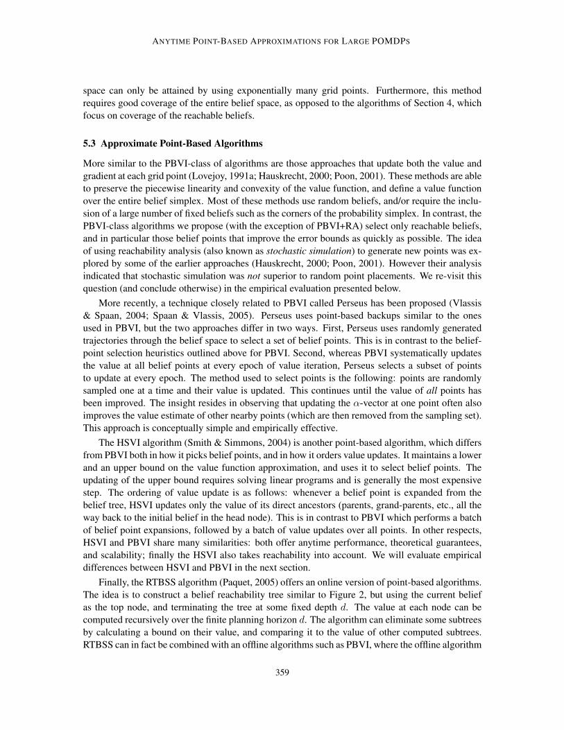
6. Experimental Evaluation
This section looks at a variety of simulated POMDP domains to evaluate the empirical performanceof PBVI. The first three domains—Tiger-grid, Hallway, Hallway2—are extracted from the estab-lished POMDP literature (Cassandra, 1999). The fourth—Tag—was introduced in some of ourearlier work as a new challenge for POMDP algorithms.
The first goal of these experiments is to establish the scalability of the PBVI framework; this isaccomplished by showing that PBVI-type algorithms can successfully solve problems in excess of800 states. We also demonstrate that PBVI algorithms compare favorably to alternative approximatevalue iteration methods. Finally, following on the example of Section 4.6, we study at a larger scalethe impact of the belief selection strategy, which confirms the superior performance of the GERstrategy.
6.1 Maze Problems
There exists a set of benchmark problems commonly used to evaluate POMDP planning algo-rithms (Cassandra, 1999). This section presents results demonstrating the performance of PBVI-class algorithms on some of those problems. While these benchmark problems are relatively small(at most 92 states, 5 actions, and 17 observations) compared to most robotics planning domains,they are useful from an analysis point of view and for comparison to previous work.
The initial performance analysis focuses on three well-known problems from the POMDP liter-ature: Tiger-grid (also known as Maze33), Hallway, and Hallway2. All three are maze navigationproblems of various sizes. The problems are fully described by Littman, Cassandra, and Kaelbling(1995a); parameterization is available from Cassandra (1999).
Figure 6a presents results for the Tiger-grid domain. Replicating earlier experiments by Braf-man (1997), test runs terminate after 500 steps (there’s an automatic reset every time the goal isreached) and results are averaged over 151 runs.
Figures 6b and 6c present results for the Hallway and Hallway2 domains, respectively. In thiscase, test runs are terminated when the goal is reached or after 251 steps (whichever occurs first),and the results are averaged over 251 runs. This is consistent with earlier experiments by Littman,Cassandra, and Kaelbling (1995b).
All three figures compare the performance of three different algorithms:
1. PBVI with Greedy Error Reduction (GER) belief point selection (Section 4.5).
2. QMDP (Littman et al., 1995b),
3. Incremental Pruning (Cassandra, Littman, & Zhang, 1997),
The QMDP heuristic (Littman et al., 1995b) takes into account partial observability at the cur-rent step, but assumes full observability on subsequent steps:
πQMDP (b) = argmaxa∈A
∑s∈S
b(s)QMDP (s, a). (39)
360

ANYTIME POINT-BASED APPROXIMATIONS FOR LARGE POMDPS
The resulting policy has some ability to resolve uncertainty, but cannot benefit from long-terminformation gathering, or compare actions with different information potential. QMDP can be seenas providing a good performance baseline. For the three problems considered, it finds a policyextremely quickly, but the policy is clearly sub-optimal.
At the other end of the spectrum, the Incremental Pruning algorithm (Zhang & Liu, 1996; Cas-sandra et al., 1997) is a direct extension of the enumeration algorithm described above. The princi-pal insight is that the pruning of dominated α-vectors (Eqn 19) can be interleaved directly with thecross-sum operator (Eqn 16). The resulting value function is the same, but the algorithm is moreefficient because it discards unnecessary vectors earlier on. While Incremental Pruning algorithmcan theoretically find an optimal policy, for the three problems considered here it would take far toolong. In fact, only a few iterations of exact backups were completed in reasonable time. In all threeproblems, the resulting short-horizon policy was worse than the corresponding PBVI policy.
As shown in Figure 6, PBVI+GER provides a much better time/performance trade-off. It findspolicies that are better than those obtained with QMDP, and does so in a matter of seconds, therebydemonstrating that it does not suffer from the same paralyzing complexity as Incremental Pruning.
While those who take a closer look at these results may be surprised to see that the performanceof PBVI actually decreases at some points (e.g., the “dip” in Fig. 6c), this is not unexpected. Itis important to remember that the theoretical properties of PBVI only guarantee a bound on theestimate of the value function, but as shown here, this does not necessarily imply that the policyneeds to improve monotonically. Nonetheless, as the value function converges, so will the policy(albeit at a slower rate).
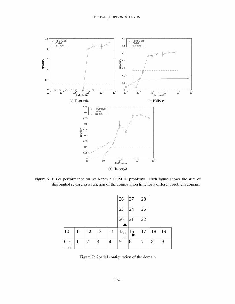
6.2 Tag Problem
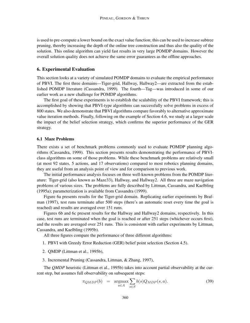
While the previous section establishes the good performance of PBVI on some well-known simu-lation problems, these are quite small and do not fully demonstrate the scalability of the algorithm.To provide a better understanding of PBVI’s effectiveness for large problems, this section presentsresults obtained when applying PBVI to the Tag problem, a robot version of the popular game oflasertag. In this problem, the agent must navigate its environment with the goal of searching for,and tagging, a moving target (Rosencrantz, Gordon, & Thrun, 2003). Real-world versions of thisproblem can take many forms, and in Section 7 we present a similar problem domain where aninteractive service robot must find an elderly patient roaming the corridors of a nursing home.
The synthetic scenario considered here is an order of magnitude larger (870 states) than mostother POMDP benchmarks in the literature (Cassandra, 1999). When formulated as a POMDP prob-lem, the goal is for the robot to optimize a policy allowing it to quickly find the person, assumingthat the person moves (stochastically) according to a fixed policy. The spatial configuration of theenvironment used throughout this experiment is illustrated in Figure 7.
The state space is described by the cross-product of two position features, Robot ={s0, . . . , s29} and Person = {s0, . . . , s29, sfound}. Both start in independently-selected randompositions, and the scenario finishes when Person = sfound. The robot can select from five actions:{North, South, East, West, Tag}. A reward of −1 is imposed for each motion action; the Tag actionresults in a +10 reward if the robot and person are in the same cell, or −10 otherwise. Through-out the scenario, the Robot’s position is fully observable, and a Move action has the predictabledeterministic effect, e. g.:
Pr(Robot = s10 | Robot = s0, North) = 1,
361
PINEAU, GORDON & THRUN
10−2
10−1
100
101
102
103
0
0.5
1
1.5
2
2.5
TIME (secs)
RE
WA
RD
PBVI+GERQMDPIncPrune
10−2
10−1
100
101
102
103
0
0.5
1
1.5
2
2.5
TIME (secs)
RE
WA
RD
PBVI+GERQMDPIncPrune
(a) Tiger-grid
10−2
10−1
100
101
102
103
0
0.1
0.2
0.3
0.4
0.5
0.6
0.7
TIME (secs)
RE
WA
RD
PBVI+GERQMDPIncPrune
(b) Hallway
10−2
10−1
100
101
102
0
0.05
0.1
0.15
0.2
0.25
0.3
0.35
0.4
0.45
TIME (secs)
RE
WA
RD
PBVI+GERQMDPIncPrune
(c) Hallway2
Figure 6: PBVI performance on well-known POMDP problems. Each figure shows the sum ofdiscounted reward as a function of the computation time for a different problem domain.
7
17
4
15
26 27
252423
20 21 22
28
5 8
18 19
9
16
6
1413
3
12
2
11
10
10
Figure 7: Spatial configuration of the domain
362
ANYTIME POINT-BASED APPROXIMATIONS FOR LARGE POMDPS
and so on for each adjacent cell and direction. The position of the person, on the other hand,is completely unobservable unless both agents are in the same cell. Meanwhile at each step, theperson (with omniscient knowledge) moves away from the robot with Pr = 0.8 and stays in placewith Pr = 0.2, e. g.:
Pr(Person = s16 | Person = s15&Robot = s0) = 0.4Pr(Person = s20 | Person = s15&Robot = s0) = 0.4Pr(Person = s15 | Person = s15&Robot = s0) = 0.2.
Figure 8 shows the performance of PBVI with Greedy Error Reduction on the Tag domain. Re-sults are averaged over 1000 runs, using different (randomly chosen) start positions for each run.The QMDP approximation is also tested to provide a baseline comparison. The results show a grad-ual improvement in PBVI’s performance as samples are added (each shown data point represents anew expansion of the belief set with value backups). It also confirms that computation time is di-rectly related to the number of belief points. PBVI requires fewer than 100 belief points to overcomeQMDP, and the performance keeps on improving as more points are added. Performance appears tobe converging with approximately 250 belief points. These results show that a PBVI-class algorithmcan effectively tackle a problem with 870 states.
100
101
102
103
104
105
−20
−18
−16
−14
−12
−10
−8
−6
TIME (secs)
RE
WA
RD
PBVI+GERQMDP
Figure 8: PBVI performance on Tag problem. We show the sum of discounted reward as a functionof the computation time.
This problem is far beyond the reach of the Incremental Pruning algorithm. A single iteration ofoptimal value iteration on a problem of this size could produce over 1020 α-vectors before pruning.Therefore, it was not applied.
This section describes one version of the Tag problem, which was used for simulation purposesin our work and that of others (Braziunas & Boutilier, 2004; Poupart & Boutilier, 2004; Smith &Simmons, 2004; Vlassis & Spaan, 2004). In fact, the problem can be re-formulated in a varietyof ways to accommodate different environments, person motion models, and observation models.Section 7 discusses variations on this problem using more realistic robot and person models, andpresents results validated onboard an independently developed robot simulator.
363
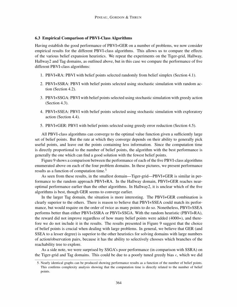
PINEAU, GORDON & THRUN
6.3 Empirical Comparison of PBVI-Class Algorithms
Having establish the good performance of PBVI+GER on a number of problems, we now considerempirical results for the different PBVI-class algorithms. This allows us to compare the effectsof the various belief expansion heuristics. We repeat the experiments on the Tiger-grid, Hallway,Hallway2 and Tag domains, as outlined above, but in this case we compare the performance of fivedifferent PBVI-class algorithms:
1. PBVI+RA: PBVI with belief points selected randomly from belief simplex (Section 4.1).
2. PBVI+SSRA: PBVI with belief points selected using stochastic simulation with random ac-tion (Section 4.2).
3. PBVI+SSGA: PBVI with belief points selected using stochastic simulation with greedy action(Section 4.3).
4. PBVI+SSEA: PBVI with belief points selected using stochastic simulation with exploratoryaction (Section 4.4).
5. PBVI+GER: PBVI with belief points selected using greedy error reduction (Section 4.5).
All PBVI-class algorithms can converge to the optimal value function given a sufficiently largeset of belief points. But the rate at which they converge depends on their ability to generally pickuseful points, and leave out the points containing less information. Since the computation timeis directly proportional to the number of belief points, the algorithm with the best performance isgenerally the one which can find a good solution with the fewest belief points.
Figure 9 shows a comparison between the performance of each of the five PBVI-class algorithmsenumerated above on each of the four problem domains. In these pictures, we present performanceresults as a function of computation time.5
As seen from these results, in the smallest domain—Tiger-grid—PBVI+GER is similar in per-formance to the random approach PBVI+RA. In the Hallway domain, PBVI+GER reaches near-optimal performance earlier than the other algorithms. In Hallway2, it is unclear which of the fivealgorithms is best, though GER seems to converge earlier.
In the larger Tag domain, the situation is more interesting. The PBVI+GER combination isclearly superior to the others. There is reason to believe that PBVI+SSEA could match its perfor-mance, but would require on the order of twice as many points to do so. Nonetheless, PBVI+SSEAperforms better than either PBVI+SSRA or PBVI+SSGA. With the random heuristic (PBVI+RA),the reward did not improve regardless of how many belief points were added (4000+), and there-fore we do not include it in the results. The results presented in Figure 9 suggest that the choiceof belief points is crucial when dealing with large problems. In general, we believe that GER (andSSEA to a lesser degree) is superior to the other heuristics for solving domains with large numbersof action/observation pairs, because it has the ability to selectively chooses which branches of thereachability tree to explore.
As a side note, we were surprised by SSGA’s poor performance (in comparison with SSRA) onthe Tiger-grid and Tag domains. This could be due to a poorly tuned greedy bias ε, which we did
5. Nearly identical graphs can be produced showing performance results as a function of the number of belief points.This confirms complexity analysis showing that the computation time is directly related to the number of beliefpoints.
364
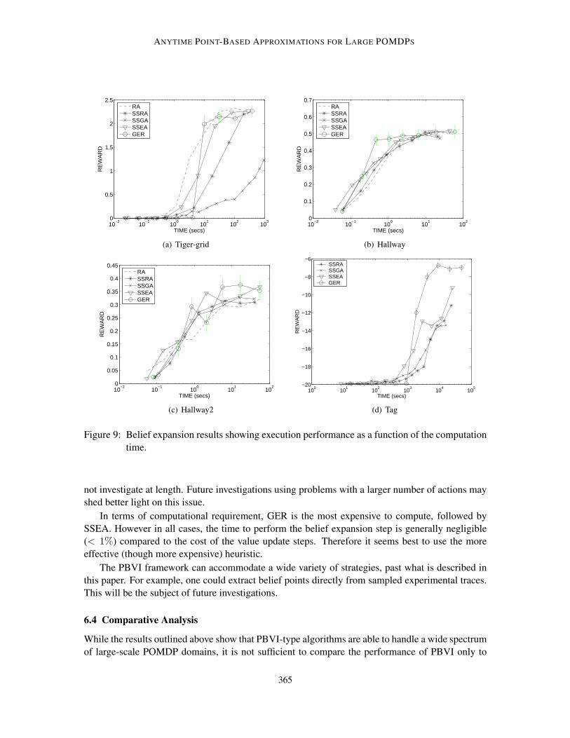
ANYTIME POINT-BASED APPROXIMATIONS FOR LARGE POMDPS
10−2
10−1
100
101
102
103
0
0.5
1
1.5
2
2.5
TIME (secs)
RE
WA
RD
RASSRASSGASSEAGER
(a) Tiger-grid
10−2
10−1
100
101
102
0
0.1
0.2
0.3
0.4
0.5
0.6
0.7
TIME (secs)
RE
WA
RD
RASSRASSGASSEAGER
(b) Hallway
10−2
10−1
100
101
102
0
0.05
0.1
0.15
0.2
0.25
0.3
0.35
0.4
0.45
TIME (secs)
RE
WA
RD
RASSRASSGASSEAGER
(c) Hallway2
100
101
102
103
104
105
−20
−18
−16
−14
−12
−10
−8
−6
TIME (secs)
RE
WA
RD
SSRASSGASSEAGER
(d) Tag
Figure 9: Belief expansion results showing execution performance as a function of the computationtime.
not investigate at length. Future investigations using problems with a larger number of actions mayshed better light on this issue.
In terms of computational requirement, GER is the most expensive to compute, followed bySSEA. However in all cases, the time to perform the belief expansion step is generally negligible(< 1%) compared to the cost of the value update steps. Therefore it seems best to use the moreeffective (though more expensive) heuristic.
The PBVI framework can accommodate a wide variety of strategies, past what is described inthis paper. For example, one could extract belief points directly from sampled experimental traces.This will be the subject of future investigations.
6.4 Comparative Analysis
While the results outlined above show that PBVI-type algorithms are able to handle a wide spectrumof large-scale POMDP domains, it is not sufficient to compare the performance of PBVI only to
365
PINEAU, GORDON & THRUN
QMDP and Incremental Pruning—the two ends of the spectrum—as done in Section 6.1. In factthere has been significant activity in recent years in the development of fast approximate POMDPalgorithms, and so it is worthwhile to spend some time comparing the PBVI framework to thesealternative approaches. This is made easy by the fact that many of these have been validated usingthe same set of problems as described above.
Table 8 summarizes the performance of a large number of recent POMDP approximation algo-rithms, including PBVI, on the four target domains: Tiger-grid, Hallway, Hallway2, and Tag. Thealgorithms listed were selected based on the availability of comparable published results or availablecode, or in some cases because the algorithm could be re-implemented easily.
We compare their empirical performance, in terms of execution performance versus planning,on a set of simulation domains. However as is often the case, these results show that there is not asingle algorithm that is best for solving all problems. We therefore also compile a summary of theattributes and characteristics of each algorithm, in an attempt to tell which algorithm may be bestfor what types of problems. Table 8 includes (whenever possible) the goal completion rates, sumof rewards, policy computation time, number of required belief points, and policy size (number ofα-vectors, or number of nodes in finite state controllers). The number of belief points and policysize are often identical, however the latter can be smaller if a single α-vector is best for multiplebelief points.
The results marked [*] were computed by us on a 3GHz Pentium 4; other results were likelycomputed on different platforms, and therefore time comparisons may be approximate at best.Nonetheless the number of samples and the size of the final policy are both useful indicators ofcomputation time. The results reported for PBVI correspond to the earliest data point from Fig-ures 6 and 8 where PBVI+GER achieves top performance.
Algorithms are listed in order of performance, starting with the algorithm(s) achieving the high-est reward. All results assume a standard (not lookahead) controller (see Hauskrecht, 2000, fordefinition).
Overall, the results indicate that some of the algorithms achieve sub-par performance in terms ofexpected reward. In the case of QMDP, this is because of fundamental limitations in the algorithm.While Incremental Pruning and the exact value-directed compression can theoretically reach optimalperformance, they would require longer computation time to do so. The grid method (see Tiger-gridresults), BPI (see Tiger-grid, Hallway and Tag results) and PBUA (see Tag results) suffer from asimilar problem, but offer much more graceful performance degradation. It is worth noting that noneof these approaches assumes a known initial belief, so in effect they are solving harder problems.The results for BBSLS are not sufficiently extensive to comment at length, but it appears to be ableto find reasonable policies with small controllers (see Tag results).
The remaining algorithms—HSVI, Perseus, and our own PBVI+GER—all offer comparableperformance on these relatively large POMDP domains. HSVI seems to offer good control perfor-mance on the full range of tasks, but requires bigger controllers, and is therefore probably slower,especially on domains with high stochasticity (e.g., Tiger-grid, Hallway, Hallway2). The trade-offsbetween Perseus and PBVI+GER are less clear: the planning time, controller size and performancequality are quite comparable, and in fact the two approaches are very similar. Similarities anddifferences between the two approaches are explored further in Section 7.
366
ANYTIME POINT-BASED APPROXIMATIONS FOR LARGE POMDPS
Method Goal% Reward ± Conf.Int. Time(s) |B| |π|Tiger-Grid (Maze33)HSVI (Smith & Simmons, 2004) n.a. 2.35 10341 n.v. 4860Perseus (Vlassis & Spaan, 2004) n.a. 2.34 104 10000 134PBUA (Poon, 2001) n.a. 2.30 12116 660 n.v.PBVI+GER[*] n.a. 2.27 ± 0.13 397 512 508BPI (Poupart & Boutilier, 2004) n.a. 1.81 163420 n.a. 1500Grid (Brafman, 1997) n.a. 0.94 n.v. 174 n.a.QMDP (Littman et al., 1995b)[*] n.a. 0.276 0.02 n.a. 5IncPrune (Cassandra et al., 1997)[*] n.a. 0.0 24hrs+ n.a. n.v.Exact VDC (Poupart & Boutilier, 2003)[*] n.a. 0.0 24hrs+ n.a. n.v.HallwayPBUA (Poon, 2001) 100 0.53 450 300 n.v.HSVI (Smith & Simmons, 2004) 100 0.52 10836 n.v. 1341PBVI+GER[*] 100 0.51 ± 0.03 19 64 64Perseus (Vlassis & Spaan, 2004) n.v. 0.51 35 10000 55BPI (Poupart & Boutilier, 2004) n.v. 0.51 249730 n.a. 1500QMDP (Littman et al., 1995b)[*] 51 0.265 0.03 n.a. 5Exact VDC (Poupart & Boutilier, 2003)[*] 39 0.161 24hrs+ n.a. n.v.IncPrune (Cassandra et al., 1997)[*] 39 0.161 24hrs+ n.a. n.v.Hallway2PBVI+GER[*] 100 0.37 ± 0.04 6 32 31Perseus (Vlassis & Spaan, 2004) n.v. 0.35 10 10000 56HSVI (Smith & Simmons, 2004) 100 0.35 10010 n.v. 1571PBUA (Poon, 2001) 100 0.35 27898 1840 n.v.BPI (Poupart & Boutilier, 2004) n.v. 0.28 274280 n.a. 1500Grid (Brafman, 1997) 98 n.v. n.v. 337 n.a.QMDP (Littman et al., 1995b)[*] 22 0.109 1.44 n.a. 5Exact VDC (Poupart & Boutilier, 2003)[*] 48 0.137 24hrs+ n.a. n.v.IncPrune (Cassandra et al., 1997)[*] 48 0.137 24hrs+ n.a. n.v.TagHSVI (Smith & Simmons, 2004) 100 -6.37 10113 n.v. 1657PBVI+GER[*] 100 -6.75 ± 0.39 8946 256 203Perseus (Vlassis & Spaan, 2004) n.v. -6.85 3076 10000 205BBSLS (Braziunas & Boutilier, 2004) n.v. -8.31 100054 n.a. 30BPI (Poupart & Boutilier, 2004) n.v. -9.18 59772 n.a. 940QMDP (Littman et al., 1995b)[*] 19 -16.62 1.33 n.a. 5PBUA (Poon, 2001)[*] 0 -19.9 24hrs+ 4096 n.v.IncPrune (Cassandra et al., 1997)[*] 0 -19.9 24hrs+ n.a. n.v.n.a.=not applicable n.v.=not available [*]=results computed by us
Table 8: Results of PBVI for standard POMDP domains
367
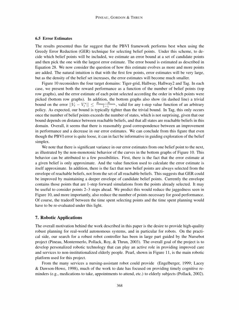
PINEAU, GORDON & THRUN
6.5 Error Estimates
The results presented thus far suggest that the PBVI framework performs best when using theGreedy Error Reduction (GER) technique for selecting belief points. Under this scheme, to de-cide which belief points will be included, we estimate an error bound at a set of candidate pointsand then pick the one with the largest error estimate. The error bound is estimated as described inEquation 28. We now consider the question of how this estimate evolves as more and more pointsare added. The natural intuition is that with the first few points, error estimates will be very large,but as the density of the belief set increases, the error estimates will become much smaller.
Figure 10 reconsiders the four target domains: Tiger-grid, Hallway, Hallway2 and Tag. In eachcase, we present both the reward performance as a function of the number of belief points (toprow graphs), and the error estimate of each point selected according the order in which points werepicked (bottom row graphs). In addition, the bottom graphs also show (in dashed line) a trivialbound on the error ||Vt − V ∗
t || ≤ Rmax−Rmin1−γ , valid for any t-step value function of an arbitrary
policy. As expected, our bound is typically tighter than the trivial bound. In Tag, this only occursonce the number of belief points exceeds the number of states, which is not surprising, given that ourbound depends on distance between reachable beliefs, and that all states are reachable beliefs in thisdomain. Overall, it seems that there is reasonably good correspondence between an improvementin performance and a decrease in our error estimates. We can conclude from this figure that eventhough the PBVI error is quite loose, it can in fact be informative in guiding exploration of the beliefsimplex.
We note that there is significant variance in our error estimates from one belief point to the next,as illustrated by the non-monotonic behavior of the curves in the bottom graphs of Figure 10. Thisbehavior can be attributed to a few possibilities. First, there is the fact that the error estimate ata given belief is only approximate. And the value function used to calculate the error estimate isitself approximate. In addition, there is the fact that new belief points are always selected from theenvelope of reachable beliefs, not from the set of all reachable beliefs. This suggests that GER couldbe improved by maintaining a deeper envelope of candidate belief points. Currently the envelopecontains those points that are 1-step forward simulations from the points already selected. It maybe useful to consider points 2–3 steps ahead. We predict this would reduce the jaggedness seen inFigure 10, and more importantly, also reduce the number of points necessary for good performance.Of course, the tradeoff between the time spent selecting points and the time spent planning wouldhave to be re-evaluated under this light.
7. Robotic Applications
The overall motivation behind the work described in this paper is the desire to provide high-qualityrobust planning for real-world autonomous systems, and in particular for robots. On the practi-cal side, our search for a robust robot controller has been in large part guided by the Nursebotproject (Pineau, Montermerlo, Pollack, Roy, & Thrun, 2003). The overall goal of the project is todevelop personalized robotic technology that can play an active role in providing improved careand services to non-institutionalized elderly people. Pearl, shown in Figure 11, is the main roboticplatform used for this project.
From the many services a nursing-assistant robot could provide (Engelberger, 1999; Lacey& Dawson-Howe, 1998), much of the work to date has focused on providing timely cognitive re-minders (e.g., medications to take, appointments to attend, etc.) to elderly subjects (Pollack, 2002).
368
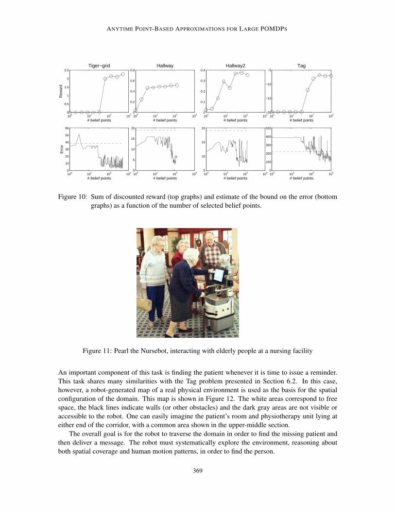
ANYTIME POINT-BASED APPROXIMATIONS FOR LARGE POMDPS
100
101
102
103
0
0.5
1
1.5
2
2.5
# belief points
Rew
ard
Tiger−grid
100
101
102
103
0
10
20
30
40
50
60
# belief points
Err
or
100
101
102
103
0
0.2
0.4
0.6
0.8
# belief points
Hallway
100
101
102
103
0
5
10
15
20
# belief points
100
101
102
103
0
0.1
0.2
0.3
0.4
# belief points
Hallway2
100
101
102
103
5
10
15
20
# belief points
100
101
102
103
−20
−15
−10
−5
# belief points
Tag
100
101
102
103
0
100
200
300
400
500
# belief points
Figure 10: Sum of discounted reward (top graphs) and estimate of the bound on the error (bottomgraphs) as a function of the number of selected belief points.
Figure 11: Pearl the Nursebot, interacting with elderly people at a nursing facility
An important component of this task is finding the patient whenever it is time to issue a reminder.This task shares many similarities with the Tag problem presented in Section 6.2. In this case,however, a robot-generated map of a real physical environment is used as the basis for the spatialconfiguration of the domain. This map is shown in Figure 12. The white areas correspond to freespace, the black lines indicate walls (or other obstacles) and the dark gray areas are not visible oraccessible to the robot. One can easily imagine the patient’s room and physiotherapy unit lying ateither end of the corridor, with a common area shown in the upper-middle section.
The overall goal is for the robot to traverse the domain in order to find the missing patient andthen deliver a message. The robot must systematically explore the environment, reasoning aboutboth spatial coverage and human motion patterns, in order to find the person.
369
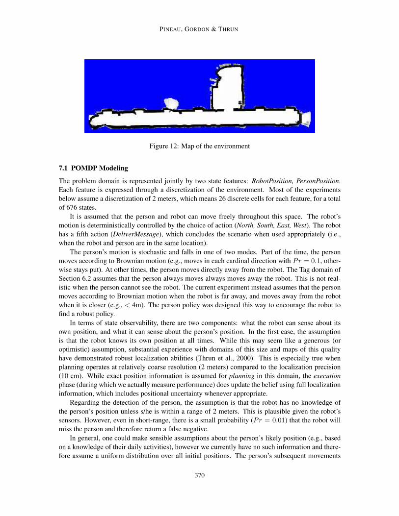
PINEAU, GORDON & THRUN
Figure 12: Map of the environment
7.1 POMDP Modeling
The problem domain is represented jointly by two state features: RobotPosition, PersonPosition.Each feature is expressed through a discretization of the environment. Most of the experimentsbelow assume a discretization of 2 meters, which means 26 discrete cells for each feature, for a totalof 676 states.
It is assumed that the person and robot can move freely throughout this space. The robot’smotion is deterministically controlled by the choice of action (North, South, East, West). The robothas a fifth action (DeliverMessage), which concludes the scenario when used appropriately (i.e.,when the robot and person are in the same location).
The person’s motion is stochastic and falls in one of two modes. Part of the time, the personmoves according to Brownian motion (e.g., moves in each cardinal direction with Pr = 0.1, other-wise stays put). At other times, the person moves directly away from the robot. The Tag domain ofSection 6.2 assumes that the person always moves always moves away the robot. This is not real-istic when the person cannot see the robot. The current experiment instead assumes that the personmoves according to Brownian motion when the robot is far away, and moves away from the robotwhen it is closer (e.g., < 4m). The person policy was designed this way to encourage the robot tofind a robust policy.
In terms of state observability, there are two components: what the robot can sense about itsown position, and what it can sense about the person’s position. In the first case, the assumptionis that the robot knows its own position at all times. While this may seem like a generous (oroptimistic) assumption, substantial experience with domains of this size and maps of this qualityhave demonstrated robust localization abilities (Thrun et al., 2000). This is especially true whenplanning operates at relatively coarse resolution (2 meters) compared to the localization precision(10 cm). While exact position information is assumed for planning in this domain, the executionphase (during which we actually measure performance) does update the belief using full localizationinformation, which includes positional uncertainty whenever appropriate.
Regarding the detection of the person, the assumption is that the robot has no knowledge ofthe person’s position unless s/he is within a range of 2 meters. This is plausible given the robot’ssensors. However, even in short-range, there is a small probability (Pr = 0.01) that the robot willmiss the person and therefore return a false negative.
In general, one could make sensible assumptions about the person’s likely position (e.g., basedon a knowledge of their daily activities), however we currently have no such information and there-fore assume a uniform distribution over all initial positions. The person’s subsequent movements
370
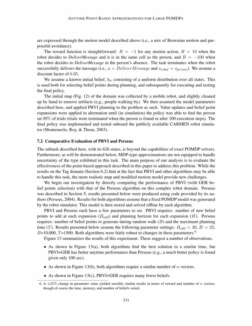
ANYTIME POINT-BASED APPROXIMATIONS FOR LARGE POMDPS
are expressed through the motion model described above (i.e., a mix of Brownian motion and pur-poseful avoidance).
The reward function is straightforward: R = −1 for any motion action, R = 10 when therobot decides to DeliverMessage and it is in the same cell as the person, and R = −100 whenthe robot decides to DeliverMessage in the person’s absence. The task terminates when the robotsuccessfully delivers the message (i.e., a = DeliverMessage and srobot = sperson). We assume adiscount factor of 0.95.
We assume a known initial belief, b0, consisting of a uniform distribution over all states. Thisis used both for selecting belief points during planning, and subsequently for executing and testingthe final policy.
The initial map (Fig. 12) of the domain was collected by a mobile robot, and slightly cleanedup by hand to remove artifacts (e.g., people walking by). We then assumed the model parametersdescribed here, and applied PBVI planning to the problem as such. Value updates and belief pointexpansions were applied in alternation until (in simulation) the policy was able to find the personon 99% of trials (trials were terminated when the person is found or after 100 execution steps). Thefinal policy was implemented and tested onboard the publicly available CARMEN robot simula-tor (Montemerlo, Roy, & Thrun, 2003).
7.2 Comparative Evaluation of PBVI and Perseus
The subtask described here, with its 626 states, is beyond the capabilities of exact POMDP solvers.Furthermore, as will be demonstrated below, MDP-type approximations are not equipped to handleuncertainty of the type exhibited in this task. The main purpose of our analysis is to evaluate theeffectiveness of the point-based approach described in this paper to address this problem. While theresults on the Tag domain (Section 6.2) hint at the fact that PBVI and other algorithms may be ableto handle this task, the more realistic map and modified motion model provide new challenges.
We begin our investigation by directly comparing the performance of PBVI (with GER be-lief points selection) with that of the Perseus algorithm on this complex robot domain. Perseuswas described in Section 5; results presented below were produced using code provided by its au-thors (Perseus, 2004). Results for both algorithms assume that a fixed POMDP model was generatedby the robot simulator. This model is then stored and solved offline by each algorithm.
PBVI and Perseus each have a few parameters to set. PBVI requires: number of new beliefpoints to add at each expansion (Badd) and planning horizon for each expansion (H). Perseusrequires: number of belief points to generate during random walk (B) and the maximum planningtime (T ). Results presented below assume the following parameter settings: Badd = 30, H = 25,B=10,000, T=1500. Both algorithms were fairly robust to changes in these parameters.6
Figure 13 summarizes the results of this experiment. These suggest a number of observations.
• As shown in Figure 13(a), both algorithms find the best solution in a similar time, butPBVI+GER has better anytime performance than Perseus (e.g., a much better policy is foundgiven only 100 sec).
• As shown in Figure 13(b), both algorithms require a similar number of α-vectors.
• As shown in Figure 13(c), PBVI+GER requires many fewer beliefs.
6. A ±25% change in parameter value yielded sensibly similar results in terms of reward and number of α vectors,though of course the time, memory, and number of beliefs varied.
371
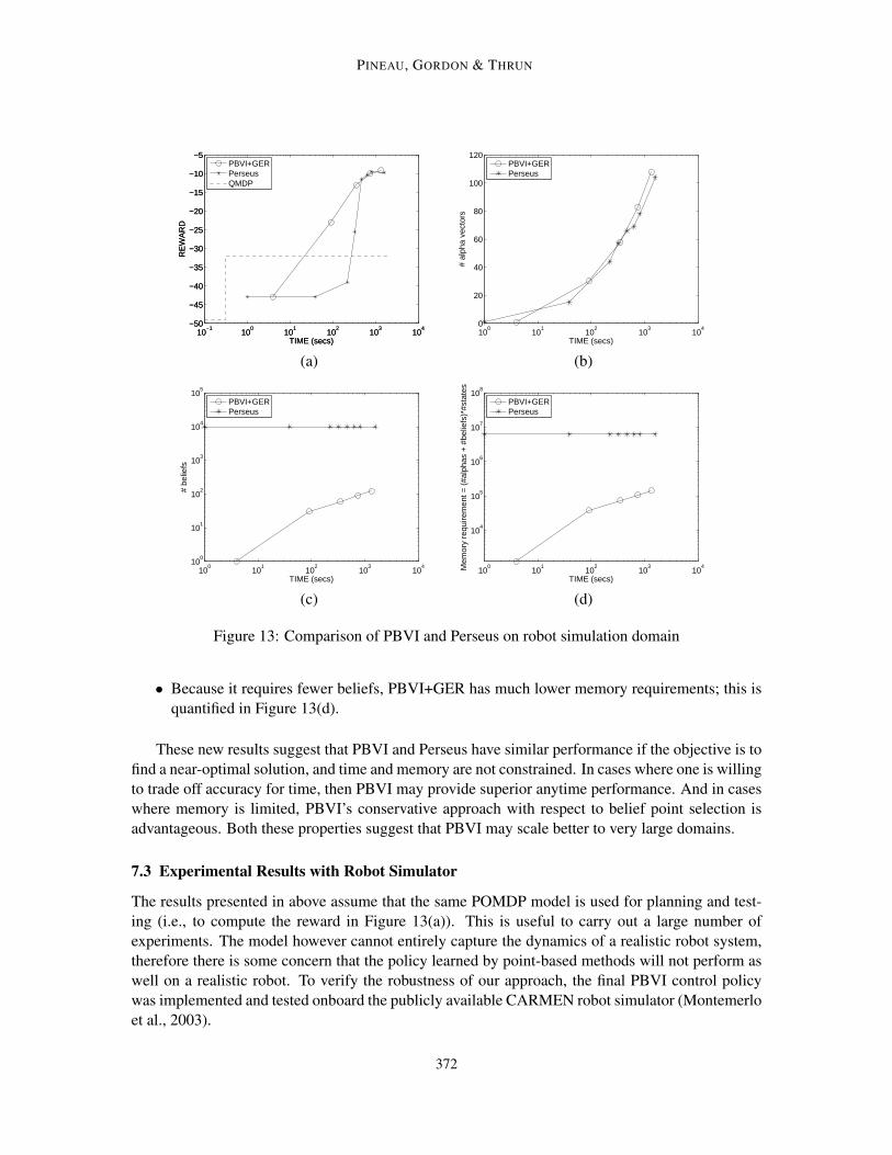
PINEAU, GORDON & THRUN
10−1
100
101
102
103
104
−50
−45
−40
−35
−30
−25
−20
−15
−10
−5
TIME (secs)
RE
WA
RD
GERPerseusQMDP
10−1
100
101
102
103
104
−50
−45
−40
−35
−30
−25
−20
−15
−10
−5
TIME (secs)
RE
WA
RD
PBVI+GERPerseusQMDP
100
101
102
103
104
0
20
40
60
80
100
120
TIME (secs)
# al
pha
vect
ors
PBVI+GERPerseus
(a) (b)
100
101
102
103
104
100
101
102
103
104
105
TIME (secs)
# be
liefs
PBVI+GERPerseus
100
101
102
103
104
104
105
106
107
108
TIME (secs)
Mem
ory
requ
irem
ent =
(#a
lpha
s +
#be
liefs
)*#s
tate
s
PBVI+GERPerseus
(c) (d)
Figure 13: Comparison of PBVI and Perseus on robot simulation domain
• Because it requires fewer beliefs, PBVI+GER has much lower memory requirements; this isquantified in Figure 13(d).
These new results suggest that PBVI and Perseus have similar performance if the objective is tofind a near-optimal solution, and time and memory are not constrained. In cases where one is willingto trade off accuracy for time, then PBVI may provide superior anytime performance. And in caseswhere memory is limited, PBVI’s conservative approach with respect to belief point selection isadvantageous. Both these properties suggest that PBVI may scale better to very large domains.
7.3 Experimental Results with Robot Simulator
The results presented in above assume that the same POMDP model is used for planning and test-ing (i.e., to compute the reward in Figure 13(a)). This is useful to carry out a large number ofexperiments. The model however cannot entirely capture the dynamics of a realistic robot system,therefore there is some concern that the policy learned by point-based methods will not perform aswell on a realistic robot. To verify the robustness of our approach, the final PBVI control policywas implemented and tested onboard the publicly available CARMEN robot simulator (Montemerloet al., 2003).
372
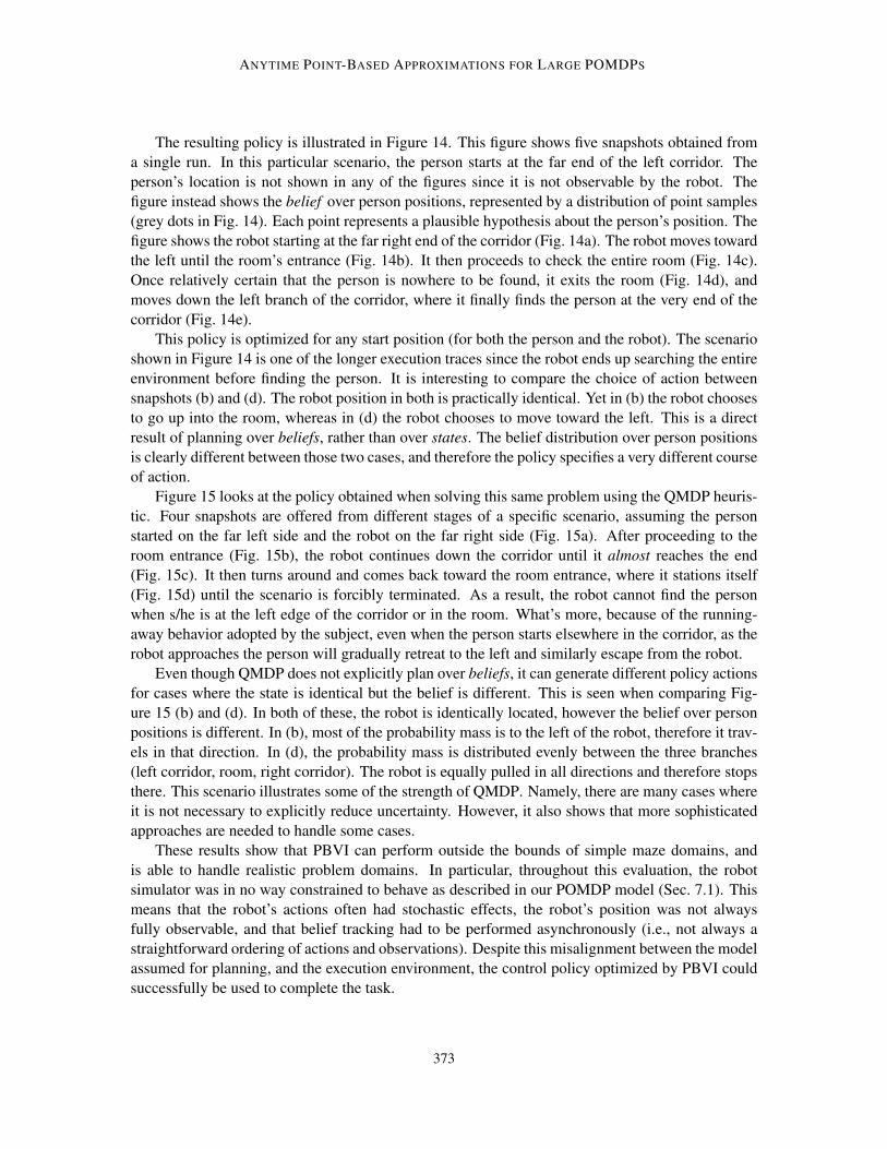
ANYTIME POINT-BASED APPROXIMATIONS FOR LARGE POMDPS
The resulting policy is illustrated in Figure 14. This figure shows five snapshots obtained froma single run. In this particular scenario, the person starts at the far end of the left corridor. Theperson’s location is not shown in any of the figures since it is not observable by the robot. Thefigure instead shows the belief over person positions, represented by a distribution of point samples(grey dots in Fig. 14). Each point represents a plausible hypothesis about the person’s position. Thefigure shows the robot starting at the far right end of the corridor (Fig. 14a). The robot moves towardthe left until the room’s entrance (Fig. 14b). It then proceeds to check the entire room (Fig. 14c).Once relatively certain that the person is nowhere to be found, it exits the room (Fig. 14d), andmoves down the left branch of the corridor, where it finally finds the person at the very end of thecorridor (Fig. 14e).
This policy is optimized for any start position (for both the person and the robot). The scenarioshown in Figure 14 is one of the longer execution traces since the robot ends up searching the entireenvironment before finding the person. It is interesting to compare the choice of action betweensnapshots (b) and (d). The robot position in both is practically identical. Yet in (b) the robot choosesto go up into the room, whereas in (d) the robot chooses to move toward the left. This is a directresult of planning over beliefs, rather than over states. The belief distribution over person positionsis clearly different between those two cases, and therefore the policy specifies a very different courseof action.
Figure 15 looks at the policy obtained when solving this same problem using the QMDP heuris-tic. Four snapshots are offered from different stages of a specific scenario, assuming the personstarted on the far left side and the robot on the far right side (Fig. 15a). After proceeding to theroom entrance (Fig. 15b), the robot continues down the corridor until it almost reaches the end(Fig. 15c). It then turns around and comes back toward the room entrance, where it stations itself(Fig. 15d) until the scenario is forcibly terminated. As a result, the robot cannot find the personwhen s/he is at the left edge of the corridor or in the room. What’s more, because of the running-away behavior adopted by the subject, even when the person starts elsewhere in the corridor, as therobot approaches the person will gradually retreat to the left and similarly escape from the robot.
Even though QMDP does not explicitly plan over beliefs, it can generate different policy actionsfor cases where the state is identical but the belief is different. This is seen when comparing Fig-ure 15 (b) and (d). In both of these, the robot is identically located, however the belief over personpositions is different. In (b), most of the probability mass is to the left of the robot, therefore it trav-els in that direction. In (d), the probability mass is distributed evenly between the three branches(left corridor, room, right corridor). The robot is equally pulled in all directions and therefore stopsthere. This scenario illustrates some of the strength of QMDP. Namely, there are many cases whereit is not necessary to explicitly reduce uncertainty. However, it also shows that more sophisticatedapproaches are needed to handle some cases.
These results show that PBVI can perform outside the bounds of simple maze domains, andis able to handle realistic problem domains. In particular, throughout this evaluation, the robotsimulator was in no way constrained to behave as described in our POMDP model (Sec. 7.1). Thismeans that the robot’s actions often had stochastic effects, the robot’s position was not alwaysfully observable, and that belief tracking had to be performed asynchronously (i.e., not always astraightforward ordering of actions and observations). Despite this misalignment between the modelassumed for planning, and the execution environment, the control policy optimized by PBVI couldsuccessfully be used to complete the task.
373
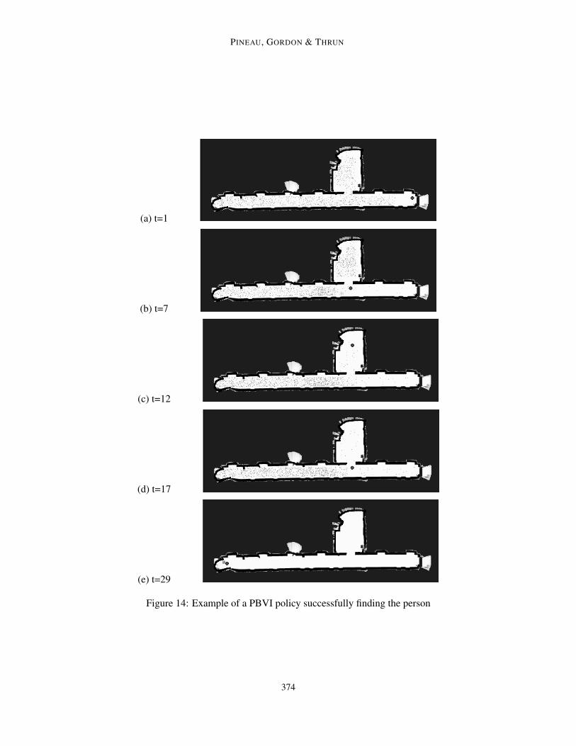
PINEAU, GORDON & THRUN
(a) t=1
(b) t=7
(c) t=12
(d) t=17
(e) t=29
Figure 14: Example of a PBVI policy successfully finding the person
374
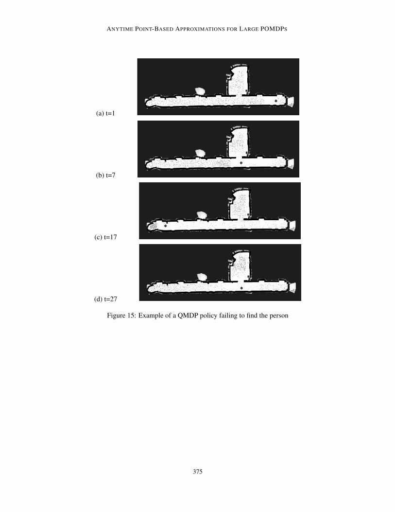
ANYTIME POINT-BASED APPROXIMATIONS FOR LARGE POMDPS
(a) t=1
(b) t=7
(c) t=17
(d) t=27
Figure 15: Example of a QMDP policy failing to find the person
375
PINEAU, GORDON & THRUN
8. Discussion
This paper describes a class of anytime point-based POMDP algorithms called PBVI, which com-bines point-based value updates with strategic selection of belief points, to solve large POMDPs.Further extensions to the PBVI framework, whereby value updates are applied to groups of beliefpoints according to their spatial distribution, are described by (Pineau, Gordon, & Thrun, 2004).The main contributions pertaining to the PBVI framework are now summarized.
Scalability. The PBVI framework is an important step towards truly scalable POMDP solutions.This is achieved by bounding the policy size through the selection of a small set of belief points.
Anytime planning. PBVI-class algorithms alternates between steps of value updating and stepsof belief point selection. As new points are added, the solution improves, at the expense of increasedcomputational time. The trade-off can be controlled by adjusting the number of points. The algo-rithm can be terminated either when a satisfactory solution is found, or when planning time iselapsed.
Bounded error. We provide a theoretical bound on the error of the approximation introducedin the PBVI framework. This result holds for a range of belief point selection methods, and leaddirectly to the development of a new PBVI-type algorithm: PBVI+GER, where estimates of theerror bound are used directly to select belief points. Furthermore we find that the bounds can beuseful in assessing when to stop adding belief points.
Exploration. We proposed a set of new point selection heuristics, which explore the tree ofreachable beliefs to select useful belief points. The most successful technique described, GreedyError Reduction (GER), uses an estimate of the error bound on candidate belief points to select themost useful points.
Improved empirical performance. PBVI has demonstrated the ability to reduce planning timefor a number of well-known POMDP problems, including Tiger-grid, Hallway, and Hallway2. Byoperating on a set of discrete points, PBVI algorithms can perform polynomial-time value updates,thereby overcoming the curse of history that paralyzes exact algorithms. The GER technique used toselect points allows us to solve large problems with fewer belief points than alternative approaches.
New problem domain. PBVI was applied to a new POMDP planning domain (Tag), for whichit generated an approximate solution that outperformed baseline algorithms QMDP and IncrementalPruning. This new domain has since been adopted as a test case for other algorithms (Vlassis &Spaan, 2004; Smith & Simmons, 2004; Braziunas & Boutilier, 2004; Poupart & Boutilier, 2004).This fosters an increased ease of comparison between new techniques. Further comparative analysiswas provided in Section 7.2 highlighting similarities and differences between PBVI and Perseus.
Demonstrated performance. PBVI was applied in the context of a robotic search-and-rescuetype scenario, where a mobile robot is required to search its environment and find a non-stationaryindividual. PBVI’s performance was evaluated using a realistic, independently-developed, robotsimulator.
A significant portion of this paper is dedicated to a thorough comparative analysis of point-basedmethods. This includes evaluating a range of point-based selection methods, as well as evaluatingmechanisms for ordering value updates. The comparison of point-based selection techniques sug-gest that the GER method presented in Section 4.5 is superior to more naive techniques. In terms ofordering of value updates, the randomized strategy which is used in the Perseus algorithm appearseffective to accelerate planning. A natural next step would be to combine the GER belief selectionheuristic with Perseus’s random value updates. We performed experiments along these lines, but
376
ANYTIME POINT-BASED APPROXIMATIONS FOR LARGE POMDPS
did not achieve any significant speed-up over the current performance of PBVI or Perseus (e.g., asreported in Figure 13(a)). It is likely that when belief points are chosen carefully (as in GER), eachof these points needs to be updated systematically and therefore there is no additional benefit tousing randomized value updates.
Looking towards the future, it is important to remember that while we have demonstrated theability to solve problems which are large by POMDP standards, many real-world domains far exceedthe complex of domains considered in this paper. In particular, it is not unusual for a problem to beexpressed through a number of multi-valued state features, in which case the number of states growsexponentially with the number of features. This is of concern because each belief point and eachα-vector has dimensionality |S| (where |S| is the number of states) and all dimensions are updatedsimultaneously. This is an important issue to address to improve the scalability of point-based valueapproaches in general.
There are various existing attempts at overcoming the curse of dimensionality in POMDPs.Some of these—e. g. the belief compression techniques by Roy and Gordon (2003)—cannot beincorporated within the PBVI framework without compromising its theoretical properties (as dis-cussed in Section 3). Others, in particular the exact compression algorithm by Poupart and Boutilier(2003), can be combined with PBVI. However, preliminary experiments in this direction haveyielded little performance improvement. There is reason to believe that approximate value com-pression would yield better results, but again at the expense of forgoing PBVI’s theoretical proper-ties. The challenge therefore is to devise function-approximation techniques that both reduce thedimensionality effectively, while maintaining the convexity properties of the solution.
A secondary (but no less important) issue concerning the scalability of PBVI pertains to thenumber of belief points necessary to obtain a good solution. While problems addressed thus far canusually be solved with O(|S|) belief points, this need not be true. In the worse case, the numberof belief points necessary may be exponential in the plan length. The PBVI framework can accom-modate a wide variety of strategies for generating belief points, and the Greedy Error Reductiontechnique seems particularly effective. However this is unlikely to be the definitive answer to beliefpoint selection. In more general terms, this relates closely to the well-known issue of explorationversus exploitation, which arises across a wide array of problem-solving techniques.
These promising opportunities for future research aside, the PBVI framework has alreadypushed the envelope of POMDP problems that can be solved with existing computational resources.As the field of POMDPs matures, finding ways of computing policies efficiently will likely continueto be a major bottleneck. We hope that point based algorithms such as the PBVI will play a leadingrole in the search for more efficient algorithms.
Acknowledgments
The authors wish to thank Craig Boutilier, Michael Littman, Andrew Moore and Matthew Mason formany thoughtful comments and discussions regarding this work. We also thank Darius Braziunas,Pascal Poupart, Trey Smith and Nikos Vlassis, for conversations regarding their algorithms andresults. The contributions of Michael Montemerlo and Nicholas Roy in conducting the empiricalrobot evaluations are gratefully acknowledged. Finally, we thank three anonymous reviewers andone dedicated editor (Sridhar Mahadevan) whose feedback significantly improved the paper. Thiswork was funded through the DARPA MARS program and NSF’s ITR program (Project: ”RoboticAssistants for the Elderly”, PI: J. Dunbar-Jacob).
377
PINEAU, GORDON & THRUN
References
Astrom, K. J. (1965). Optimal control of markov decision processes with incomplete state estima-tion. Journal of Mathematical Analysis and Applications, 10, 174–205.
Bellman, R. (1957). Dynamic Programming. Princeton University Press.
Bertsekas, D. P., & Tsitsiklis, J. (1996). Neuro-Dynamic Programming. Athena Scientific.
Blum, A. L., & Furst, M. L. (1997). Fast planning through planning graph analysis. ArtificialIntelligence, 90(1-2), 281–300.
Bonet, B. (2002). An epsilon-optimal grid-based algorithm for partially obserable Markov decisionprocesses. In Machine Learning: Proceedings of the 2002 International Conference (ICML),pp. 51–58.
Boutilier, C., Dean, T., & Hanks, S. (1999). Decision-theoretic planning: Structural assumptionsand computational leverage. Journal of Artificial Intelligence Research, 11, 1–94.
Boyen, X., & Koller, D. (1998). Tractable inference for complex stochastic processes. In Proceed-ings of the Fourteenth Conference on Uncertainty in Artificial Intelligence (UAI), pp. 33–42.
Brafman, R. I. (1997). A heuristic variable grid solution method for POMDPs. In Proceedings ofthe Fourteenth National Conference on Artificial Intelligence (AAAI), pp. 727–733.
Braziunas, D., & Boutilier, C. (2004). Stochastic local search for POMDP controllers. In Proceed-ings of the Nineteenth National Conference on Artificial Intelligence (AAAI), pp. 690–696.
Burgard, W., Cremers, A. B., Fox, D., Hahnel, D., Lakemeyer, G., Schulz, D., Steiner, W., & Thrun,S. (1999). Experiences with an interactive museum tour-guide robot. Artificial Intelligence,114, 3–55.
Cassandra, A. (1999). Tony’s POMDP page. http://www.cs.brown.edu/research/ai/pomdp/code/index.html.
Cassandra, A., Littman, M. L., & Zhang, N. L. (1997). Incremental pruning: A simple, fast, exactmethod for partially observable Markov decision processes. In Proceedings of the ThirteenthConference on Uncertainty in Artificial Intelligence (UAI), pp. 54–61.
Chapman, D. (1987). Planning for conjunctive goals. Artificial Intelligence, 32(3), 333–377.
Cheng, H.-T. (1988). Algorithms for Partially Observable Markov Decision Processes. Ph.D. thesis,University of British Columbia.
Dean, T., & Kanazawa, K. (1988). Probabilistic temporal reasoning. In Proceedings of the SeventhNational Conference on Artificial Intelligence (AAAI), pp. 524–528.
Devroye, L. (1986). Non-Uniform Random Variate Generation. Springer-Verlag, New York.
Engelberger, G. (1999). Handbook of Industrial Robotics. John Wiley and Sons.
Fikes, R. E., & Nilsson, N. J. (1971). STRIPS: A new approach to the application of theoremproving to problem solving. Artificial Intelligence, 2, 189–208.
Hauskrecht, M. (1997). Incremental methods for computing bounds in partially observable Markovdecision processes. In Proceedings of the Fourteenth National Conference on Artificial Intel-ligence (AAAI), pp. 734–739.
378
ANYTIME POINT-BASED APPROXIMATIONS FOR LARGE POMDPS
Hauskrecht, M. (2000). Value-function approximations for partially observable Markov decisionprocesses. Journal of Artificial Intelligence Research, 13, 33–94.
Jazwinski, A. M. (1970). Stochastic Processes and Filtering Theory. Academic, New York.
Kaelbling, L. P., Littman, M. L., & Cassandra, A. R. (1998). Planning and acting in partiallyobservable stochastic domains. Artificial Intelligence, 101, 99–134.
Kalman, R. E. (1960). A new approach to linear filtering and prediction problems. Transactions ofthe ASME, Journal of Basic Engineering, 82, 35–45.
Lacey, G., & Dawson-Howe, K. M. (1998). The application of robotics to a mobility aid for theelderly blind. Robotics and Autonomous Systems, 23, 245–252.
Littman, M. L. (1996). Algorithms for Sequential Decision Making. Ph.D. thesis, Brown University.
Littman, M. L., Cassandra, A. R., & Kaelbling, L. P. (1995a). Learning policies for partially ob-sevable environments: Scaling up. Tech. rep. CS-95-11, Brown University, Department ofComputer Science.
Littman, M. L., Cassandra, A. R., & Kaelbling, L. P. (1995b). Learning policies for partially ob-sevable environments: Scaling up. In Proceedings of Twelfth International Conference onMachine Learning, pp. 362–370.
Lovejoy, W. S. (1991a). Computationally feasible bounds for partially observed Markov decisionprocesses. Operations Research, 39(1), 162–175.
Lovejoy, W. S. (1991b). A survey of algorithmic methods for partially observable Markov decisionprocesses. Annals of Operations Research, 28, 47–66.
McAllester, D., & Roseblitt, D. (1991). Systematic nonlinear planning. In Proceedings of the NinthNational Conference on Artificial Intelligence (AAAI), pp. 634–639.
Monahan, G. E. (1982). A survey of partially observable Markov decision processes: Theory, mod-els, and algorithms. Management Science, 28(1), 1–16.
Montemerlo, M., Roy, N., & Thrun, S. (2003). Perspectives on standardization in mobile robotprogramming: The Carnegie Mellon navigation (CARMEN) toolkit. In Proceedings of theIEEE/RSJ International Conference on Intelligent Robots and Systems (IROS), Vol. 3, pp. pp2436–2441.
Paquet, S. (2005). Distributed Decision-Making and Task Coordination in Dynamic, Uncertain andReal-Time Multiagent Environments. Ph.D. thesis, Universite Laval.
Penberthy, J. S., & Weld, D. (1992). UCPOP: A sound, complete, partial order planning for ADL.In Proceedings of the Third International Conference on Knowledge Representation and Rea-soning, pp. 103–114.
Perseus (2004) http://staff.science.uva.nl/mtjspaan/software/approx.
Pineau, J., Gordon, G., & Thrun, S. (2004). Applying metric-trees to belief-point POMDPs. InNeural Information Processing Systems (NIPS), Vol. 16.
Pineau, J., Montermerlo, M., Pollack, M., Roy, N., & Thrun, S. (2003). Towards robotic assistants innursing homes: challenges and results. Robotics and Autonomous Systems, 42(3-4), 271–281.
Pollack, M. (2002). Planning technology for intelligent cognifitve orthotics. In Proceedings of the6th International Conference on AI Planning & Scheduling (AIPS).
379
PINEAU, GORDON & THRUN
Poon, K.-M. (2001). A fast heuristic algorithm for decision-theoretic planning. Master’s thesis, TheHong-Kong University of Science and Technology.
Poupart, P., & Boutilier, C. (2000). Value-directed belief state approximation for POMDPs. InProceedings of the Sixteenth Conference on Uncertainty in Artificial Intelligence (UAI), pp.409–416.
Poupart, P., & Boutilier, C. (2003). Value-directed compression of POMDPs. In Advances in NeuralInformation Processing Systems (NIPS), Vol. 15.
Poupart, P., & Boutilier, C. (2004). Bounded finite state controllers. In Advances in Neural Infor-mation Processing Systems (NIPS), Vol. 16.
Rabiner, L. R. (1989). A tutorial on hidden Markov models and selected applications in speechrecognition. Proceedings of the IEEE, 77(2), 257–285.
Rosencrantz, M., Gordon, G., & Thrun, S. (2003). Locating moving entities in dynamic indoorenvironments with teams of mobile robots. In Second International Joint Conference onAutonomous Agents and MultiAgent Systems (AAMAS), pp. 233–240.
Roy, N., & Gordon, G. (2003). Exponential family PCA for belief compression in POMDPs. InAdvances in Neural Information Processing Systems (NIPS), Vol. 15, pp. 1043–1049.
Smith, T., & Simmons, R. (2004). Heuristic search value iteration for POMDPs. In Proceedings ofthe Twentieth Conference on Uncertainty in Artificial Intelligence (UAI).
Sondik, E. J. (1971). The Optimal Control of Partially Observable Markov Processes. Ph.D. thesis,Stanford University.
Spaan, M., & Vlassis, N. (2005). Perseus: Randomized point-based value iteration for POMDPs.Journal of Artificial Intelligence Research (JAIR), 195–220.
Sutton, R. S., & Barto, A. G. (1998). Reinforcement Learning: An Introduction. MIT Press.
Thrun, S., Fox, D., Burgard, W., & Dellaert, F. (2000). Robust Monte Carlo localization for mobilerobots. Artificial Intelligence, 128(1-2), 99–141.
Vlassis, N., & Spaan, M. T. J. (2004). A fast point-based algorithm for POMDPs. In Proceedingsof the Belgian-Dutch Conference on Machine Learning.
White, C. C. (1991). A survey of solution techniques for the partially observed Markov decisionprocess. Annals of Operations Research, 32, 215–230.
Zhang, N. L., & Liu, W. (1996). Planning in stochastic domains: Problem characteristics and ap-proximation. Tech. rep. HKUST-CS96-31, Dept. of Computer Science, Hong Kong Univer-sity of Science and Technology.
Zhang, N. L., & Zhang, W. (2001). Speeding up the convergence of value iteration in partiallyobservable Markov decision processes. Journal of Artificial Intelligence Research, 14, 29–51.
Zhou, R., & Hansen, E. A. (2001). An improved grid-based approximation algorithm for POMDPs.In Proceedings of the 17th International Joint Conference on Artificial Intelligence (IJCAI),pp. 707–716.
380