Anytime Classification Using the Nearest Neighbor …eamonn/Anytime_Classification.pdfAnytime...

Anytime Classification Using the Nearest Neighbor

Algorithm with Applications to Stream Mining

Ken Ueno

Corporate Research and Development Center

Toshiba Corporation

1 Komukai-toshiba-cho, Saiwai-ku, Kawasaki 212-8520, JAPAN

[email protected]

Xiaopeng Xi Eamonn Keogh Dah-Jye Lee1

Computer Science & Engineering Department University of California, Riverside

Riverside, CA 92521 {xxi, eamonn}@cs.ucr.edu

1Brigham Young University [email protected]

ABSTRACT For many real world problems we must perform classification under widely varying amounts of computational resources. For example, if asked to classify an instance taken from a bursty stream, we may have from milliseconds to minutes to return a class prediction. For such problems an anytime algorithm may be especially useful.

In this work we show how we can convert the ubiquitous nearest neighbor classifier into an anytime algorithm that can produce an instant classification, or if given the luxury of additional time, can utilize the extra time to increase classification accuracy. We demonstrate the utility of our approach with a comprehensive set of experiments on data from diverse domains.

Keywords Classification, Anytime Algorithms, Nearest Neighbor, Streams

1. INTRODUCTION For many real world problems we must perform classification under widely varying amounts of computational resources. For example, if asked to classify an instance taken from a bursty stream [2][29], we may have from milliseconds to minutes to return a class prediction. For such problems an anytime algorithm may be especially useful.

Anytime algorithms are algorithms that trade execution time for quality of results [8]. In particular, an anytime algorithm always has a best-so-far answer available, and the quality of the answer improves with execution time. The user may examine this answer at any time, and then choose to terminate the algorithm, temporarily suspend the algorithm, or allow the algorithm to run to completion. The utility of anytime algorithms for data mining has been extensively documented [5][6][28]. To increase the reader’s appreciation of the utility of nearest neighbor classifiers in real world settings we will consider some motivating examples below. Audio Sensor Monitoring: In ongoing work we are attempting

to build classifiers for “smart” insect traps that can identify the species and sex of automatically captured insects [33]. While

the single feature of wing beat frequency is quite effective by itself, our best results come from a nearest neighbor algorithm that considers many additional features, including sound amplitude, time of day, season, temperature, humidity etc. Our classifier must run on low-powered embedded computers attached to disposable smart traps. This computer has very limited computational resources, making exhaustive nearest neighbor search quite demanding even in databases of only a few thousand instances. Furthermore, in our empirical studies we found that the insects inter arrival time can vary from tenths of seconds to tens of minutes. In such an environment an anytime algorithm will allow the classifier to make the best possible decision in the time permitted.

Robotics: A general approach to robot navigation, (the so called SLAM problem, Simultaneous Localization And Mapping) is for the robot to perform range scans and compare the shapes to previously obtained maps [15]. However the shape comparisons can be computationally expensive [1], and the robot may be forced to move before an exhaustive nearest neighbor search has been completed. Under such circumstances an anytime algorithm will allow the robot to best utilize the time before a decision is forced.

Industrial Applications: As noted in [4] “Many industrial applications require classification of items placed on a moving conveyor”. The distance measure used may have a complexity as high as O(n3) in order to achieve robustness despite rotation and other distortions [1]. In domains such as manufacturing it may be possible to know the frequency at which the objects in question pass under the camera. However in other applications, such as fruit sorting and grading [34], the inter arrival times can vary greatly. The amount of time the algorithm has to classify an object before it must take action (i.e., blowing the suspect fruit off the conveyer with compressed air) can vary by up to 3 orders of magnitude. Once again using an anytime algorithm can allow us to make the best decision in the time available.

In this work we show how we can convert the ubiquitous nearest neighbor classifier to an anytime algorithm that can produce an instant classification, or if given the luxury of additional time, can increase classification accuracy. The framework is based on the simple intuition that important exemplars (instances highly

representative of a given class) should be examined first. We show that, for most problems, a simple generic algorithm can produce a high quality ordering of the exemplars, . We also show that, in some specialized domains, we can further improve our algorithm with domain-specific techniques. The rest of the paper is organized as follows. In Section 2, we review related work and discuss some background material. In Section 3 we introduce a formal definition of our anytime nearest neighbour classification. We introduce our observations on index ordering in Section 4. Section 5 introduces three general heuristics for ordering the instances for our algorithm. In Section 6 we show an example of a special ordering heuristic that can take advantage of domain knowledge in time series classification. We perform an extensive empirical evaluation in Section 7. In Section 8 we provide a detailed case study of a real world application of our algorithm to streaming data. Finally, Section 9 offers some conclusions and suggestions for future work.

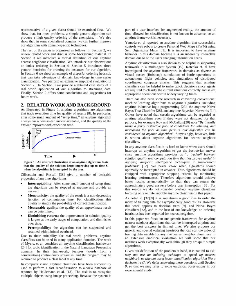
2. RELATED WORK AND BACKGROUND As illustrated in Figure 1, anytime algorithms are algorithms that trade execution time for quality of results [8]. In particular, after some small amount of “setup time,” an anytime algorithm always has a best-so-far answer available, and the quality of the answer improves with execution time.

Figure 1: An abstract illustration of an anytime algorithm. Note that the quality of the solution keeps improving up to time S, when the algorithm is interrupted by the user.

Zilberstein and Russell [38] give a number of desirable properties of anytime algorithms: • Interruptability: After some small amount of setup time,

the algorithm can be stopped at anytime and provide an answer.

• Monotonicity: the quality of the result is a non-decreasing function of computation time. For classification, this quality is simply the probability of correct classification.

• Measurable quality: the quality of an approximate result can be determined.

• Diminishing returns: the improvement in solution quality is largest at the early stages of computation, and diminishes over time.

• Preemptability: the algorithm can be suspended and resumed with minimal overhead.

Due to their suitability for real world problems, anytime classifiers can be used in many application domains. The work of Myers, et al. considers an anytime classification framework [24] for topic identification in the Natural Language Processing domains. In their framework, features (words from a conversation) continuously stream in, and the program may be required to produce a class label at any time. In computer vision anytime classifiers have been successfully used to perform a fast reconfiguration to a view database as reported by Heidemann et al. [13]. The task is to recognize multiple objects using image processing. Because the system is

part of a user interface for augmented reality, the amount of time allowed for classification is not known in advance, so an anytime framework is necessary. Yamada et. al reported an anytime algorithm that successfully controls web robots to create Personal Web Maps (PWM) using Self Organizing Maps [31]. It is important to have anytime behavior in this domain because it is an inherently interactive domain due to of the users changing information needs. Anytime classification is also shown to be helpful in supporting teamwork in a multi-agent system [19]. Kotenko et. al have investigated the anytime framework in domains as diverse as virtual soccer (Robocup), simulations of battle operations in autonomous flight vehicles, and simulations of distributed coordinated computer attacks. This suggests that anytime classifiers can be helpful to make quick decisions since agents are required to classify the current situations correctly and select appropriate operations within widely varying times. There has also been some research in converting conventional machine learning algorithms to anytime algorithms, including anytime inductive logic programming [23], the anytime Naïve Bayes Text Classifier [28], and anytime Bayesian Networks [14]. Others have noted that certain algorithms can be regarded as anytime algorithms even if they were not designed for that purpose, for example Roy and McCallum[28] note “By initially using a fairly restrictive pool of candidates for labeling, and increasing the pool as time permits, our algorithm can be considered an anytime algorithm”. Surprisingly, however, little is written about anytime algorithms for nearest neighbor classifiers.

Time

Qua

lity

of

Solu

tion Current Solution

Setup Time

STime

Qua

lity

of

Solu

tion Current Solution

Setup Time

S

In any anytime classifier, it is hard to know when users should interrupt an anytime algorithm to get the best-so-far answer since anytime algorithms provides us “a tradeoff between solution quality and computation time that has proved useful in applying artificial intelligence techniques to time-critical problems” [12]. We never know when algorithms should optimally be interrupted in advance. Thus algorithms should be equipped with appropriate stopping criteria by monitoring learning performances. Therefore algorithms should achieve better results asymptotically so that they can return the approximately good answers before user interruption [38]. For this reason we do not consider contract anytime classifiers focusing only on interruptible anytime classifiers in this paper. As noted in [32][9] it is sometimes a good idea to order the index of training data for asymptotically good results. However this work applies to decision trees [9], and Naïve Bayes classifiers [32], and to the best of our knowledge, no ordering heuristics has been reported for nearest neighbor. In this paper we focus on our generic framework for anytime nearest neighbor algorithms that can be interrupted anytime and get the best answers in limited time. We also propose our generic and special ordering heuristics that can sort the index of training data suitable for anytime nearest neighbor classifiers. In an extensive empirical evaluation we will show that our methods work exceptionally well although they are quite simple algorithms. Given our definition of the problem at hand, it is natural to ask, why not use an indexing technique to speed up nearest neighbor?, or why not use a faster classification algorithm like a decision tree?. We defer answering these questions until Section 9, so that we may refer to some empirical observations in our experimental study.

3. ANYTIME NEAREST NEIGHBOR Assume we have a set of m training instances, which we refer to as Database. We can access the ith exemplar from this set with Database.object(i), and the class label for the ith exemplar with Database.class_label(i). The instances in the database can be any objects we are interested in classifying, such as classic database tuples, strings, graphs, time series, webpages etc. Assume that Index is a permutation of the integers from 1 to m, where m is the size of Database. Finally, assume O is an object we wish to classify using an anytime nearest neighbor algorithm with Database as our training data. At some time S, where number_of_classes(Database) ≤ S ≤ m, the algorithm will be interrupted and we report a class label prediction for O. Given the above notation, Table 1 shows our anytime nearest neighbor algorithm.

Table 1: Anytime Nearest Neighbor Algorithm 1

2

3

4

5

6

7

8

9

10

11

12

13

14

15

16

17

18

19

20

21

22

23

Function [best_match_class]= Anytime_Classifier (Database, Index, O)

best_match_val = inf;

best_match_class = undefined;

For p = 1 to number_of_classes(Database)

D = distance(Database.object(Indexp) , O);

If D < best_match_val

best_match_val = D;

best_match_class = Database.class_label(Indexp);

End

End

Disp(‘The algorithm can now be interrupted’);

p = number_of_classes(Database) + 1;

While (user_has_not_interrupted AND p < max(index) )

D = distance(Database.object(Indexp) , O);

If D < best_match_val

best_match_val = D;

best_match_class = Database.class_label(Indexp);

End

p = p +1;

user_has_not_interrupted = test_for_user_interrupt;

End

In the first ten lines of code we compare O to one member of each class and tentatively assign its class label to the nearest exemplar. Note that the algorithm cannot be interrupted during this phase of the algorithm, however this is a very small amount of time. After this setup time, the algorithm can be interrupted at any point. Until it is interrupted, or has exhaustively compared O to the entire database, it will compare O to each object in the database in the order predefined in Index variable, updating the class prediction to reflect the current cumulative results. Note that we have not yet defined how Index is sorted. The only way we can help the algorithm above is to sort the Index such that “useful” examples will appear early. In Section 4 we will make some observations about this problem before introducing several concrete algorithms as solutions in Sections 5 and 6. Before leaving this section it is worth making two additional observations about the anytime algorithm. We note that the distance measure, distance(Database.object(Indexp),O) can be any distance measure, including Euclidean distance, Manhattan distance, correlation, etc. Where appropriate it can also be any specialized distance measure such as string edit

distance, Dynamic Time Warping etc. Note also that the time and space complexity for classification has not changed, although we must do some additional preprocessing work in creating the Index variable.

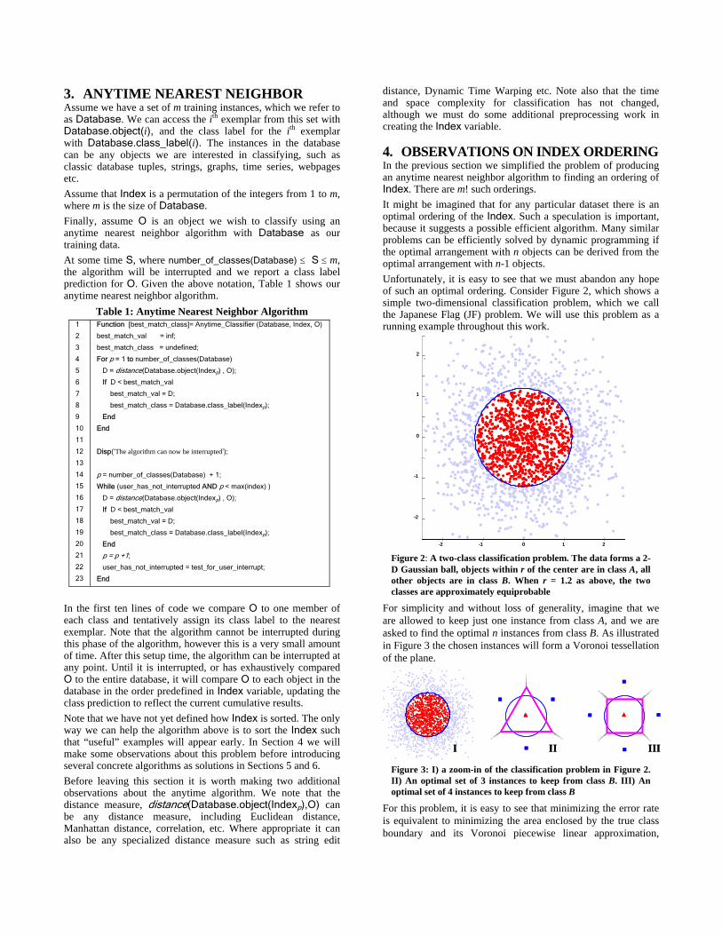
4. OBSERVATIONS ON INDEX ORDERING In the previous section we simplified the problem of producing an anytime nearest neighbor algorithm to finding an ordering of Index. There are m! such orderings. It might be imagined that for any particular dataset there is an optimal ordering of the Index. Such a speculation is important, because it suggests a possible efficient algorithm. Many similar problems can be efficiently solved by dynamic programming if the optimal arrangement with n objects can be derived from the optimal arrangement with n-1 objects. Unfortunately, it is easy to see that we must abandon any hope of such an optimal ordering. Consider Figure 2, which shows a simple two-dimensional classification problem, which we call the Japanese Flag (JF) problem. We will use this problem as a running example throughout this work.

-2 -1 0 1 2

-2

-1

0

1

2

-2 -1 0 1 2

-2

-1

0

1

2

Figure 2: A two-class classification problem. The data forms a 2-D Gaussian ball, objects within r of the center are in class A, all other objects are in class B. When r = 1.2 as above, the two classes are approximately equiprobable

For simplicity and without loss of generality, imagine that we are allowed to keep just one instance from class A, and we are asked to find the optimal n instances from class B. As illustrated in Figure 3 the chosen instances will form a Voronoi tessellation of the plane.

I II IIII II III

Figure 3: I) a zoom-in of the classification problem in Figure 2. II) An optimal set of 3 instances to keep from class B. III) An optimal set of 4 instances to keep from class B

For this problem, it is easy to see that minimizing the error rate is equivalent to minimizing the area enclosed by the true class boundary and its Voronoi piecewise linear approximation,

which in turn is equivalent to the Archimedean problem of approximating a circle with n straight lines. The implications for the task at hand are obvious. In this case the optimal 4 instances and the optimal 3 instances have zero intersections. We cannot derive the optimal arrangement for n instances from the optimal arrangement with n-1 instances. We could instead attempt to solve the problem of finding the optimal arrangement of instances, given perfect knowledge of the distribution of the interruption times. However a fundamental (and realistic) assumption of anytime algorithms is that we have no way of knowing when an interruption might take place, even on average. Note that these findings are not all bad news for us. At least for this JF problem we can see that there are many very good solutions for each value of n.

5. GENERAL ORDERING HEURISTICS Having introduced our anytime classification algorithm, we note that there are only two ways to modify the algorithm: by changing the distance measure and by changing the Index ordering heuristic. As distance measurement selection is an independent concern well-documented in many other papers, will only focus on the critical Index ordering subroutine Table 2 shows our ordering algorithm. The basic intuition is as follows: We begin by finding the “worst” exemplar (Line 4), and place a pointer to it in the last position in the Index (Line 5). To ensure that we don’t consider it again, we replace the exmplar in the original list with a null (Line 6). We then repeatedly find the worst exemplar remaining and place a pointer to it in the last unoccupied place in the Index.

Table 2: Ordering Algorithm 1

2

3

4

5

6

7

Function [Index] = Order_Index(Training_Database)

Index = create_vector_of_size(m) // m is the size of Training_Database

For p = 0 to m – (1 + number_of_classes(Training_Database))

location = find_location_of_worst_exemplar(Training_Database)

Indexm-p = location

Training_Database(location) = null;

End

The above algorithm is completely generic and self-contained, except we have not yet explained how we defined the “worst” exemplar. This is a deliberate omission, which allows us to explore many possibilities, and allows anyone to use our framework simply by creating a definition of the “worst” exemplar. Before considering this problem in the next section we will make some observations about the ordering algorithm. Note that there is no mechanism in the algorithm to force the first few exemplars pointed to by the Index to include one of each class. In practice however, this is almost always the case under any definition of exemplar quality. Notice also that we have chosen to search “worse-first,” rather than to search “best-first.” That is to say, we could in principle search in the opposite direction, find the best instance and place it in the first place in the Index, then find the next best instance and place it in the second place in the Index etc. The main reason for this decision is the difficulty in defining “best” in the early stages of the algorithm. It is hard to measure the utility of single instance in the early stages of “best-first” search because we are interested in the decision boundaries, which are defined by (at least) two instances of different classes.

5.1 Finding the Worst Exemplar We are now in a position to explain some techniques for defining the worst exemplar. Random and BestDrop are considered to allow some baseline comparison, and our method SimpleRank, is discussed last. • Random: Here the find_location_of_worst_exemplar

subroutine on line 4 of Table 2 simply returns a random number between 0 and m-1. We define this algorithm to allow a simple baseline comparison.

• BestDrop: There has been much work on data editing (numerosity reduction/condensing) for nearest neighbor classification [25][35]. Such algorithms have very similar goals to the current work, except these algorithms explicitly know in advance the stopping value S. Perhaps the most referenced work in this area is by Wilson and Martinez [35], who introduced 3 algorithms for determining the worst exemplar. All these algorithms create some list of nearest neighbors, of both the same class (associates) and of different classes (enemies), and use a weighted scoring function based on this list to determine the worst exemplar. We have implemented all three variants and we report only the best performing variant for each possible S value.

• SimpleRank: The intuition behind this algorithm is to give every instance a rank according to its contribution to the classification. We do leave-one-out 1-nearest-neighbor classification for the training data, and the rank of the instance is calculated as the following formula:

otherwise )1__/(2

)class( )(class if 1)( ∑

⎩⎨⎧

−−

==

j

j

classofnum

xxxrank (1)

where xj is an instance having x as its nearest neighbor. This ranking typically produces many ties for the worst instance, which we break by further sorting the instances by their distance to their nearest neighbor of the same class.

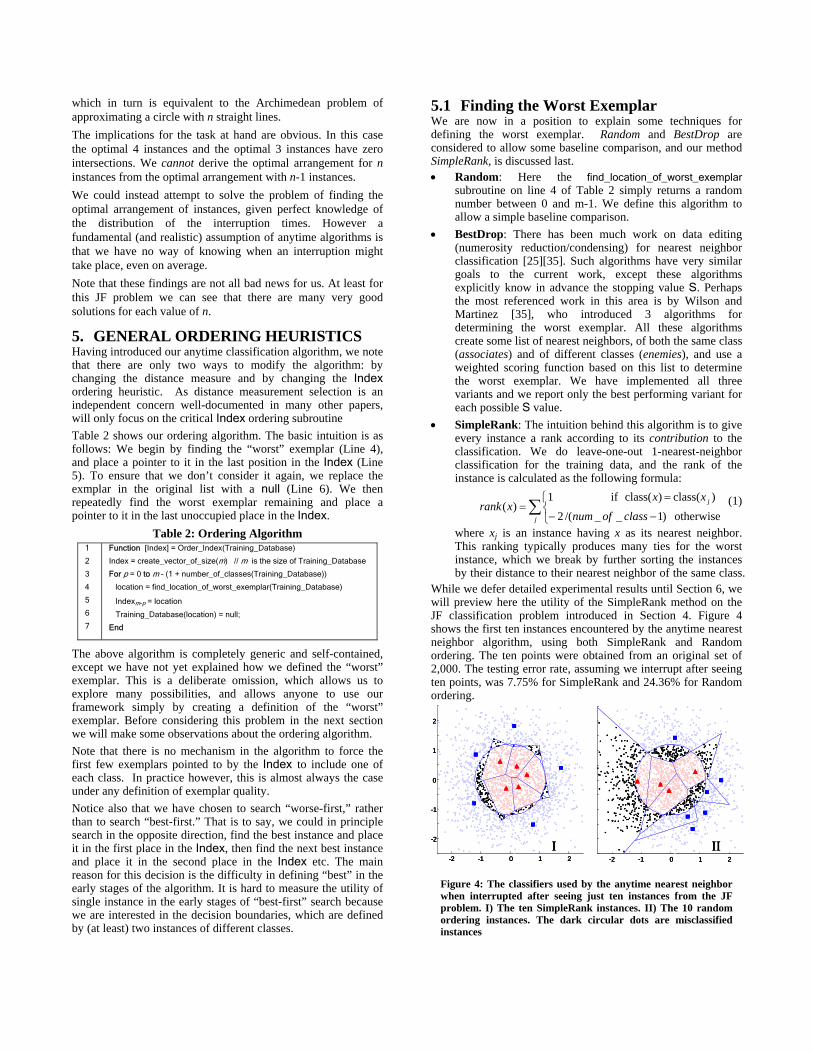
While we defer detailed experimental results until Section 6, we will preview here the utility of the SimpleRank method on the JF classification problem introduced in Section 4. Figure 4 shows the first ten instances encountered by the anytime nearest neighbor algorithm, using both SimpleRank and Random ordering. The ten points were obtained from an original set of 2,000. The testing error rate, assuming we interrupt after seeing ten points, was 7.75% for SimpleRank and 24.36% for Random ordering.

-2 -1 0 1 2I

-2

-1

0

1

2

-2 -1 0 1 2

II-2 -1 0 1 2

I-2

-1

0

1

2

-2 -1 0 1 2I

-2

-1

0

1

2

-2 -1 0 1 2

II-2 -1 0 1 2

II

Figure 4: The classifiers used by the anytime nearest neighbor when interrupted after seeing just ten instances from the JF problem. I) The ten SimpleRank instances. II) The 10 random ordering instances. The dark circular dots are misclassified instances

Note that in Figure 4 the ten instances used by SimpleRank create a decision boundary that is a pretty good approximation to the pentagon which is the optimal solution for this number of exemplars. The time complexity for a naive implementation of the ordering algorithm in Table 2 is O(m3 log(m)), because the outer loop on line 4 repeats O(m) times, and the subroutine find_location_of_worst_exemplar requires sorting m objects, after doing an all-to-all comparison. However, by simply caching the results of the first iteration of the outer loop on line 4, and only updating the instances that where affected by the temporary removal of the worse instance, we can reduce the complexity to O(m2). To concretely ground these numbers, on the largest problem considered in this work (the 11,340 training instances of the Forest Cover Type problem), the simple caching approach reduces the time complexity from 277.7 hours to 53.7 minutes using a Pentium(R)4 3.0GHz.

6. SPECIAL ORDERING HEURISTICS As we shall show in the Section 7, the generic ordering algorithms discussed in the previous section can produce dramatic improvement over random ordering. However we believe that in certain domains, it will be possible to create specialized algorithms that can then be transparently used with the anytime nearest neighbor algorithm introduced in Table 1. The specialized algorithms leverage domain-specific knowledge to produce superior results. In this section we will give one complete example of a specialized domain solution, beginning with the motivation.

6.1 Agricultural Monitoring Health care management is a critical and demanding issue in current livestock production. The economic cost related to large-scale diseases such as avian flu and BSE (“mad cow” disease) makes early detection of disease very important. This has investigated a huge effort in developing sensors and sensing techniques for diagnosis in the agricultural sector. One example of a successfully deployed system is monitoring pigs for coughing sounds indicative of certain diseases [10]. The algorithm used to detect the coughs is simple 1-nearest-neighbor with Dynamic Time Warping (DTW) as the distance measure. The system continuously monitors sounds in the pigsty to identify candidate sounds by “applying a threshold to the signal energy.” All extracted sounds are then passed to the classification system. Herein lies the problem: the DTW algorithm is relatively lethargic, requiring quadratic time per comparison, and we do not know how long we have until the next candidate sound will be extracted. This is exactly the kind of problem where an anytime algorithm is ideally suited.

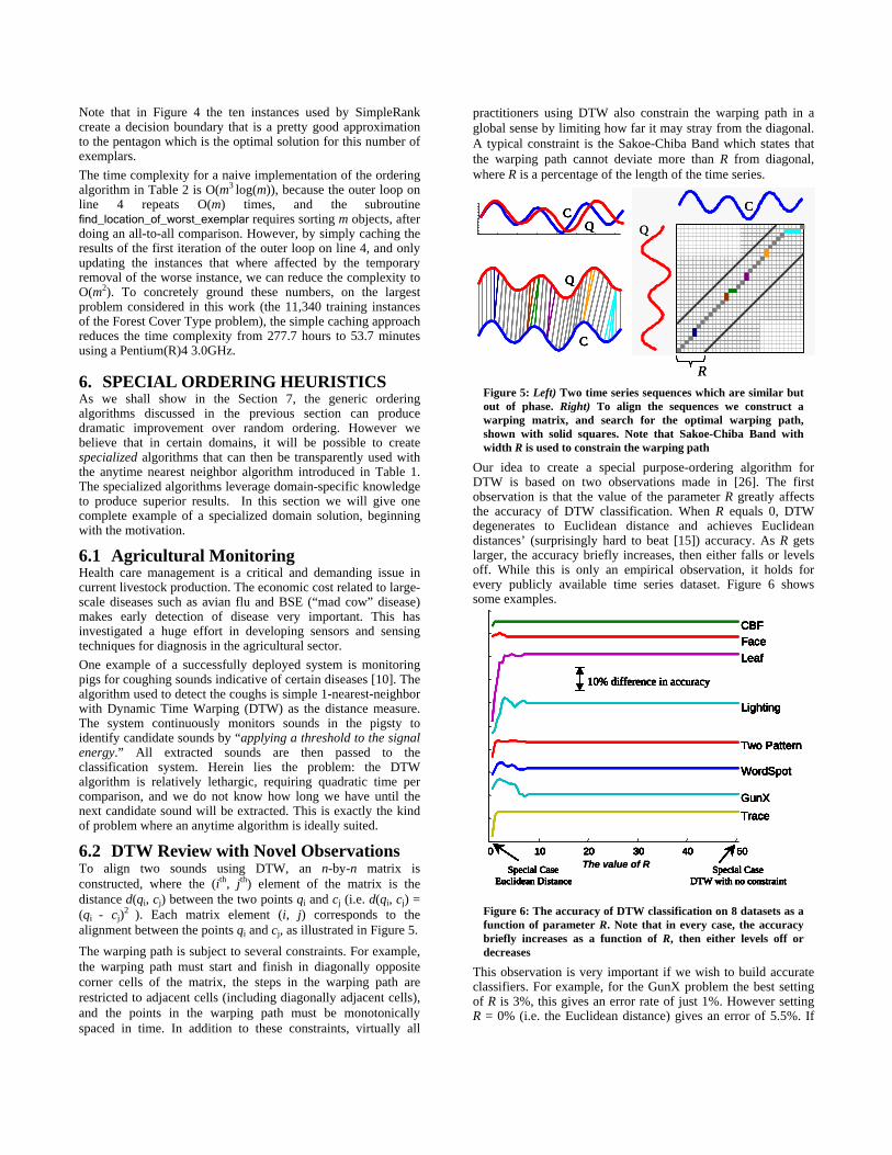
6.2 DTW Review with Novel Observations To align two sounds using DTW, an n-by-n matrix is constructed, where the (ith, jth) element of the matrix is the distance d(qi, cj) between the two points qi and cj (i.e. d(qi, cj) = (qi - cj)2 ). Each matrix element (i, j) corresponds to the alignment between the points qi and cj, as illustrated in Figure 5. The warping path is subject to several constraints. For example, the warping path must start and finish in diagonally opposite corner cells of the matrix, the steps in the warping path are restricted to adjacent cells (including diagonally adjacent cells), and the points in the warping path must be monotonically spaced in time. In addition to these constraints, virtually all

practitioners using DTW also constrain the warping path in a global sense by limiting how far it may stray from the diagonal. A typical constraint is the Sakoe-Chiba Band which states that the warping path cannot deviate more than R from diagonal, where R is a percentage of the length of the time series.

QC

QC

Q

C

QC

QC

Q

C

QC

QCC

Q

C

R

QC

QC

Q

C

QC

QC

Q

C

QC

QCC

Q

C

RFigure 5: Left) Two time series sequences which are similar but out of phase. Right) To align the sequences we construct a warping matrix, and search for the optimal warping path, shown with solid squares. Note that Sakoe-Chiba Band with width R is used to constrain the warping path

Our idea to create a special purpose-ordering algorithm for DTW is based on two observations made in [26]. The first observation is that the value of the parameter R greatly affects the accuracy of DTW classification. When R equals 0, DTW degenerates to Euclidean distance and achieves Euclidean distances’ (surprisingly hard to beat [15]) accuracy. As R gets larger, the accuracy briefly increases, then either falls or levels off. While this is only an empirical observation, it holds for every publicly available time series dataset. Figure 6 shows some examples.

0 10 20 30 40 50

CBF

GunX

Two Pattern

Trace

WordSpot

Lighting

Face

Special CaseEuclidean Distance

Special CaseDTW with no constraint

Leaf

10% difference in accuracy

0 10 20 30 40 50

CBF

The value of R

GunX

Two Pattern

Trace

WordSpot

Lighting

Face



Leaf


0 10 20 30 40 50

CBF

GunX

Two Pattern

Trace

WordSpot

Lighting

Face



Leaf


0 10 20 30 40 500 10 20 30 40 50

CBF

GunX

Two Pattern

Trace

WordSpot

Lighting

Face



Leaf


0 10 20 30 40 50

CBF

The value of R

GunX

Two Pattern

Trace

WordSpot

Lighting

Face



Leaf


0 10 20 30 40 50

CBF

GunX

Two Pattern

Trace

WordSpot

Lighting

Face



Leaf


0 10 20 30 40 50

CBF

GunX

Two Pattern

Trace

WordSpot

Lighting

Face



Leaf


Figure 6: The accuracy of DTW classification on 8 datasets as a function of parameter R. Note that in every case, the accuracy briefly increases as a function of R, then either levels off or decreases

This observation is very important if we wish to build accurate classifiers. For example, for the GunX problem the best setting of R is 3%, this gives an error rate of just 1%. However setting R = 0% (i.e. the Euclidean distance) gives an error of 5.5%. If

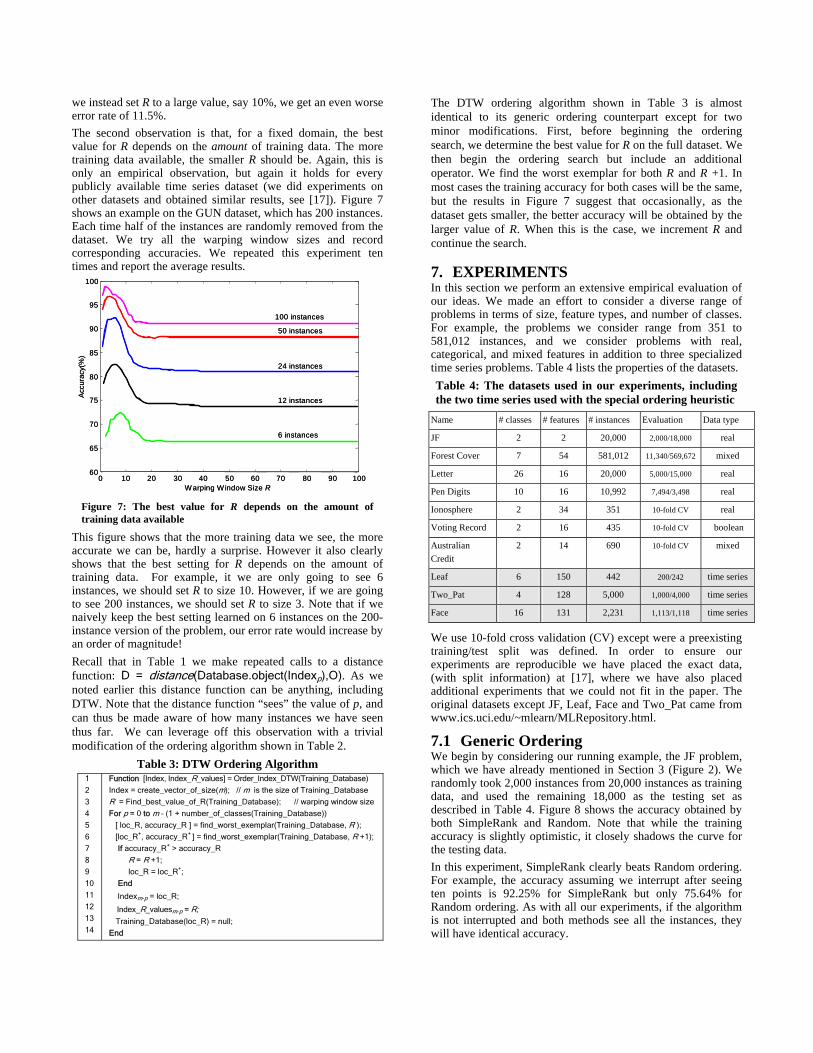
we instead set R to a large value, say 10%, we get an even worse error rate of 11.5%. The second observation is that, for a fixed domain, the best value for R depends on the amount of training data. The more training data available, the smaller R should be. Again, this is only an empirical observation, but again it holds for every publicly available time series dataset (we did experiments on other datasets and obtained similar results, see [17]). Figure 7 shows an example on the GUN dataset, which has 200 instances. Each time half of the instances are randomly removed from the dataset. We try all the warping window sizes and record corresponding accuracies. We repeated this experiment ten times and report the average results.

Figure 7: The best value for R depends on the amount of training data available

This figure shows that the more training data we see, the more accurate we can be, hardly a surprise. However it also clearly shows that the best setting for R depends on the amount of training data. For example, it we are only going to see 6 instances, we should set R to size 10. However, if we are going to see 200 instances, we should set R to size 3. Note that if we naively keep the best setting learned on 6 instances on the 200-instance version of the problem, our error rate would increase by an order of magnitude! Recall that in Table 1 we make repeated calls to a distance function: D = distance(Database.object(Indexp),O). As we noted earlier this distance function can be anything, including DTW. Note that the distance function “sees” the value of p, and can thus be made aware of how many instances we have seen thus far. We can leverage off this observation with a trivial modification of the ordering algorithm shown in Table 2.

Table 3: DTW Ordering Algorithm 1

2

3

4

5

6

7

8

9

10

11

12

13

14

Function [Index, Index_R_values] = Order_Index_DTW(Training_Database)

Index = create_vector_of_size(m); // m is the size of Training_Database

R = Find_best_value_of_R(Training_Database); // warping window size

For p = 0 to m – (1 + number_of_classes(Training_Database))

[ loc_R, accuracy_R ] = find_worst_exemplar(Training_Database, R ); [loc_R+, accuracy_R+ ] = find_worst_exemplar(Training_Database, R +1);

If accuracy_R+ > accuracy_R

R = R +1;

loc_R = loc_R+;

End

Indexm-p = loc_R;

Index_R_valuesm-p = R; Training_Database(loc_R) = null;

End

The DTW ordering algorithm shown in Table 3 is almost identical to its generic ordering counterpart except for two minor modifications. First, before beginning the ordering search, we determine the best value for R on the full dataset. We then begin the ordering search but include an additional operator. We find the worst exemplar for both R and R +1. In most cases the training accuracy for both cases will be the same, but the results in Figure 7 suggest that occasionally, as the dataset gets smaller, the better accuracy will be obtained by the larger value of R. When this is the case, we increment R and continue the search.

7. EXPERIMENTS

0 10 20 30 40 50 60 70 80 90 10060

65

70

75

80

85

90

95

100

Warping Window Size R

Acc

urac

y(%

)

6 instances

100 instances

50 instances

24 instances

12 instances

0 10 20 30 40 50 60 70 80 90 10060

65

70

75

80

85

90

95

100

Warping Window Size R

Acc

urac

y(%

)

6 instances

100 instances

50 instances

24 instances

12 instances

In this section we perform an extensive empirical evaluation of our ideas. We made an effort to consider a diverse range of problems in terms of size, feature types, and number of classes. For example, the problems we consider range from 351 to 581,012 instances, and we consider problems with real, categorical, and mixed features in addition to three specialized time series problems. Table 4 lists the properties of the datasets. Table 4: The datasets used in our experiments, including the two time series used with the special ordering heuristic

Name # classes # features # instances Evaluation Data type

JF 2 2 20,000 2,000/18,000 real

Forest Cover 7 54 581,012 11,340/569,672 mixed

Letter 26 16 20,000 5,000/15,000 real

Pen Digits 10 16 10,992 7,494/3,498 real

Ionosphere 2 34 351 10-fold CV real

Voting Record 2 16 435 10-fold CV boolean

Australian Credit

2 14 690 10-fold CV mixed

Leaf 6 150 442 200/242 time series

Two_Pat 4 128 5,000 1,000/4,000 time series

Face 16 131 2,231 1,113/1,118 time series

We use 10-fold cross validation (CV) except were a preexisting training/test split was defined. In order to ensure our experiments are reproducible we have placed the exact data, (with split information) at [17], where we have also placed additional experiments that we could not fit in the paper. The original datasets except JF, Leaf, Face and Two_Pat came from www.ics.uci.edu/~mlearn/MLRepository.html.

7.1 Generic Ordering We begin by considering our running example, the JF problem, which we have already mentioned in Section 3 (Figure 2). We randomly took 2,000 instances from 20,000 instances as training data, and used the remaining 18,000 as the testing set as described in Table 4. Figure 8 shows the accuracy obtained by both SimpleRank and Random. Note that while the training accuracy is slightly optimistic, it closely shadows the curve for the testing data. In this experiment, SimpleRank clearly beats Random ordering. For example, the accuracy assuming we interrupt after seeing ten points is 92.25% for SimpleRank but only 75.64% for Random ordering. As with all our experiments, if the algorithm is not interrupted and both methods see all the instances, they will have identical accuracy.

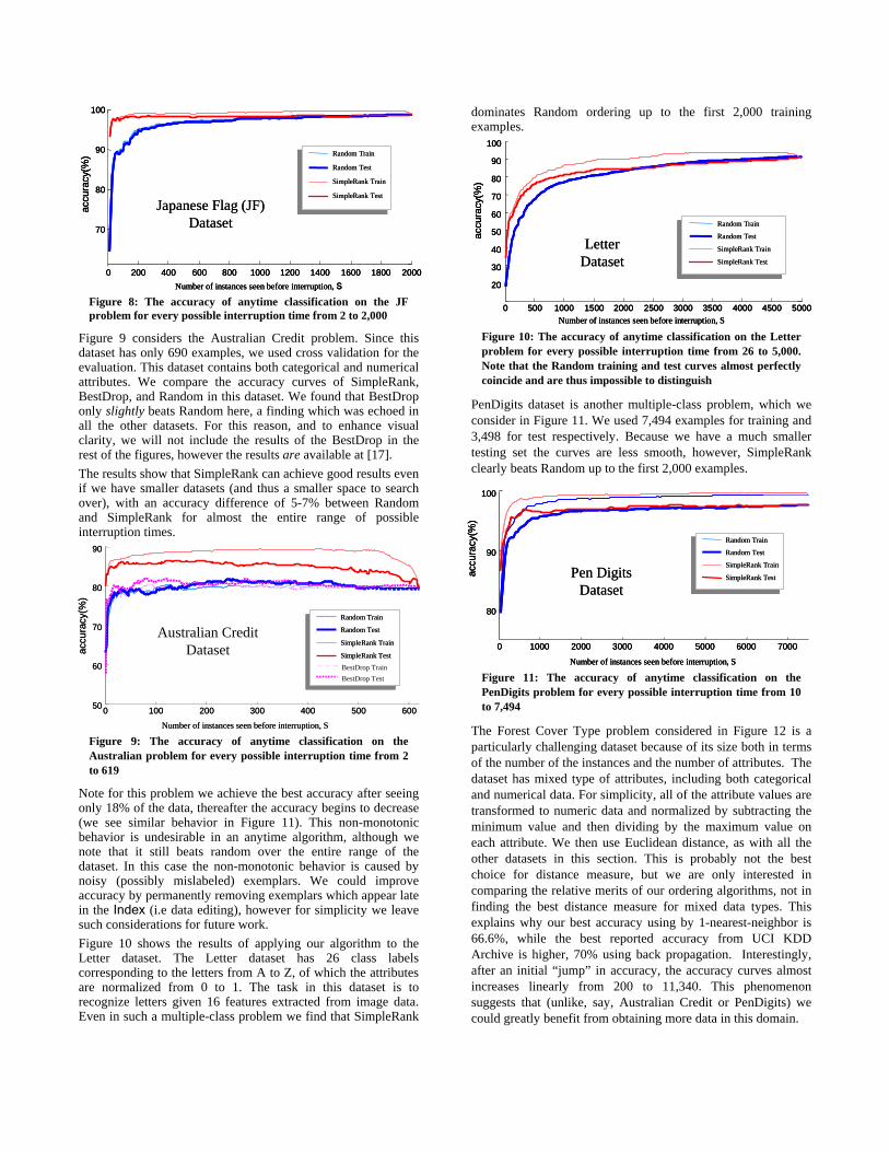
Figure 8: The accuracy of anytime classification on the JF problem for every possible interruption time from 2 to 2,000

Figure 9 considers the Australian Credit problem. Since this dataset has only 690 examples, we used cross validation for the evaluation. This dataset contains both categorical and numerical attributes. We compare the accuracy curves of SimpleRank, BestDrop, and Random in this dataset. We found that BestDrop only slightly beats Random here, a finding which was echoed in all the other datasets. For this reason, and to enhance visual clarity, we will not include the results of the BestDrop in the rest of the figures, however the results are available at [17]. The results show that SimpleRank can achieve good results even if we have smaller datasets (and thus a smaller space to search over), with an accuracy difference of 5-7% between Random and SimpleRank for almost the entire range of possible interruption times.

Figure 9: The accuracy of anytime classification on the Australian problem for every possible interruption time from 2 to 619

Note for this problem we achieve the best accuracy after seeing only 18% of the data, thereafter the accuracy begins to decrease (we see similar behavior in Figure 11). This non-monotonic behavior is undesirable in an anytime algorithm, although we note that it still beats random over the entire range of the dataset. In this case the non-monotonic behavior is caused by noisy (possibly mislabeled) exemplars. We could improve accuracy by permanently removing exemplars which appear late in the Index (i.e data editing), however for simplicity we leave such considerations for future work. Figure 10 shows the results of applying our algorithm to the Letter dataset. The Letter dataset has 26 class labels corresponding to the letters from A to Z, of which the attributes are normalized from 0 to 1. The task in this dataset is to recognize letters given 16 features extracted from image data. Even in such a multiple-class problem we find that SimpleRank

dominates Random ordering up to the first 2,000 training examples.

0 200 400 600 800 1000 1200 1400 1600 1800 2000

70

80

90

100

Number of instances seen before interruption, S

accu

racy

(%) Random Train

Random Test

SimpleRank Train

SimpleRank Test

Japanese Flag (JF) Dataset

0 200 400 600 800 1000 1200 1400 1600 1800 2000

70

80

90

100


accu

racy

(%) Random Train

Random Test

SimpleRank Train

SimpleRank Test

0 200 400 600 800 1000 1200 1400 1600 1800 2000

70

80

90

100


accu

racy

(%) Random Train

Random Test

SimpleRank Train

SimpleRank Test

Random Train

Random Test

SimpleRank Train

SimpleRank Test

Japanese Flag (JF) Dataset

50000 500 1000 1500 2000 2500 3000 3500 4000 4500

20

30

40

50

60

70

80

90

100


accu

racy

(%)

Random Train

Random Test

SimpleRank Train

SimpleRank Test

Letter Dataset

50000 500 1000 1500 2000 2500 3000 3500 4000 4500

20

30

40

50

60

70

80

90

100


accu

racy

(%)

Random Train

Random Test

SimpleRank Train

SimpleRank Test

50000 500 1000 1500 2000 2500 3000 3500 4000 4500

20

30

40

50

60

70

80

90

100


accu

racy

(%)

Random Train

Random Test

SimpleRank Train

SimpleRank Test

Random Train

Random Test

SimpleRank Train

SimpleRank Test

Letter Dataset

Figure 10: The accuracy of anytime classification on the Letter problem for every possible interruption time from 26 to 5,000. Note that the Random training and test curves almost perfectly coincide and are thus impossible to distinguish

PenDigits dataset is another multiple-class problem, which we consider in Figure 11. We used 7,494 examples for training and 3,498 for test respectively. Because we have a much smaller testing set the curves are less smooth, however, SimpleRank clearly beats Random up to the first 2,000 examples.

0 1000 2000 3000 4000 5000 6000 7000

80

90

100


accu

racy

(%)

Random Train

Random Test

SimpleRank Train

SimpleRank TestPen Digits Dataset

0 1000 2000 3000 4000 5000 6000 7000

80

90

100


accu

racy

(%)

Random Train

Random Test

SimpleRank Train

SimpleRank Test

0 1000 2000 3000 4000 5000 6000 7000

80

90

100


accu

racy

(%)

Random Train

Random Test

SimpleRank Train

SimpleRank Test

Random Train

Random Test

SimpleRank Train

SimpleRank TestPen Digits Dataset

0 100 200 300 400 500 60050

60

70

80

90


accu

racy

(%)

Random Train

Random Test

SimpleRank Train

SimpleRank Test

BestDrop TestBestDrop Train

0 100 200 300 400 500 60050

60

70

80

90


accu

racy

(%)

Random Train

Random Test

SimpleRank Train

SimpleRank Test

Random Train

Random Test

SimpleRank Train

SimpleRank Test

BestDrop TestBestDrop Train

Australian Credit Dataset

Figure 11: The accuracy of anytime classification on the PenDigits problem for every possible interruption time from 10 to 7,494

The Forest Cover Type problem considered in Figure 12 is a particularly challenging dataset because of its size both in terms of the number of the instances and the number of attributes. The dataset has mixed type of attributes, including both categorical and numerical data. For simplicity, all of the attribute values are transformed to numeric data and normalized by subtracting the minimum value and then dividing by the maximum value on each attribute. We then use Euclidean distance, as with all the other datasets in this section. This is probably not the best choice for distance measure, but we are only interested in comparing the relative merits of our ordering algorithms, not in finding the best distance measure for mixed data types. This explains why our best accuracy using by 1-nearest-neighbor is 66.6%, while the best reported accuracy from UCI KDD Archive is higher, 70% using back propagation. Interestingly, after an initial “jump” in accuracy, the accuracy curves almost increases linearly from 200 to 11,340. This phenomenon suggests that (unlike, say, Australian Credit or PenDigits) we could greatly benefit from obtaining more data in this domain.

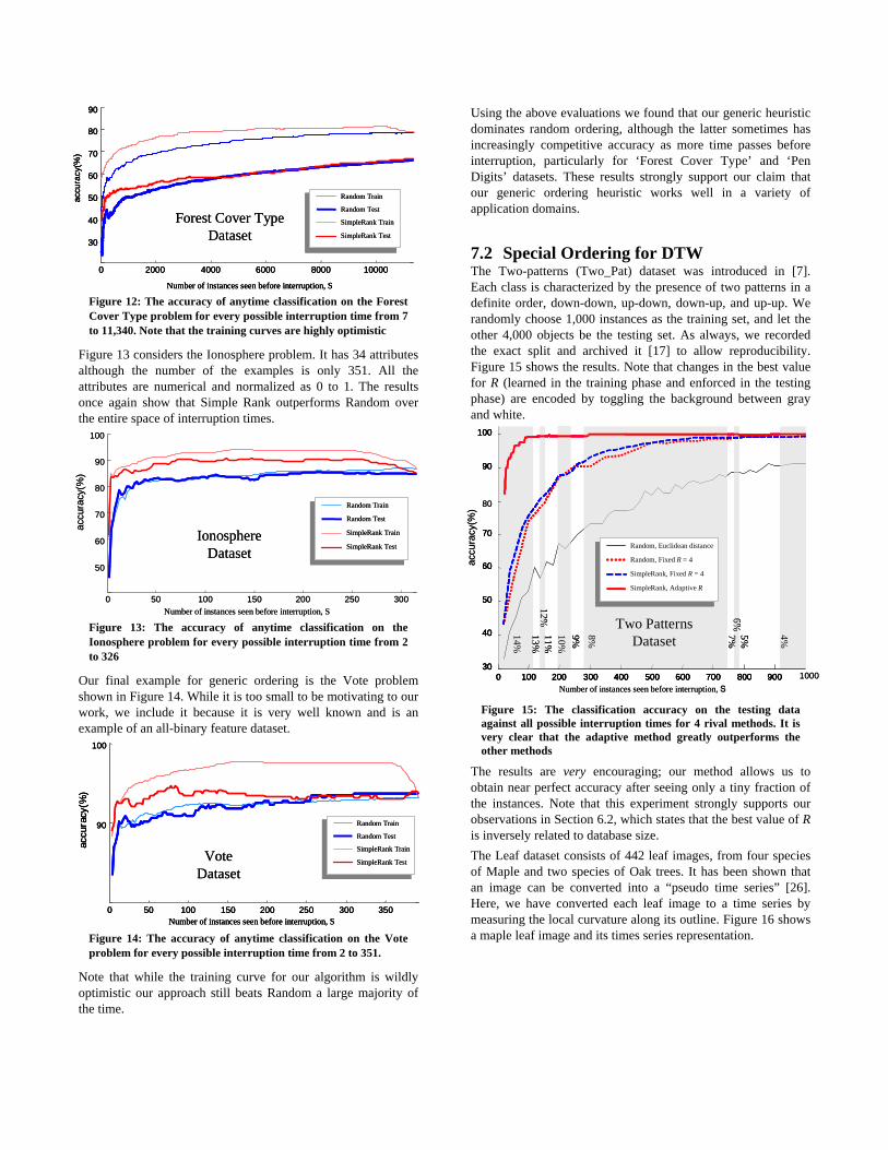
Figure 12: The accuracy of anytime classification on the Forest Cover Type problem for every possible interruption time from 7 to 11,340. Note that the training curves are highly optimistic

Figure 13 considers the Ionosphere problem. It has 34 attributes although the number of the examples is only 351. All the attributes are numerical and normalized as 0 to 1. The results once again show that Simple Rank outperforms Random over the entire space of interruption times.

Figure 13: The accuracy of anytime classification on the Ionosphere problem for every possible interruption time from 2 to 326

Our final example for generic ordering is the Vote problem shown in Figure 14. While it is too small to be motivating to our work, we include it because it is very well known and is an example of an all-binary feature dataset.

Figure 14: The accuracy of anytime classification on the Vote problem for every possible interruption time from 2 to 351.

Note that while the training curve for our algorithm is wildly optimistic our approach still beats Random a large majority of the time.

Using the above evaluations we found that our generic heuristic dominates random ordering, although the latter sometimes has increasingly competitive accuracy as more time passes before interruption, particularly for ‘Forest Cover Type’ and ‘Pen Digits’ datasets. These results strongly support our claim that our generic ordering heuristic works well in a variety of application domains.

0 2000 4000 6000 8000 10000

30

40

50

60

70

80

90


accu

racy

(%)

Random Train

Random Test

SimpleRank Train

SimpleRank Test

Forest Cover Type Dataset

0 2000 4000 6000 8000 10000

30

40

50

60

70

80

90


accu

racy

(%)

Random Train

Random Test

SimpleRank Train

SimpleRank Test

0 2000 4000 6000 8000 10000

30

40

50

60

70

80

90


accu

racy

(%)

Random Train

Random Test

SimpleRank Train

SimpleRank Test

Random Train

Random Test

SimpleRank Train

SimpleRank Test

Forest Cover Type Dataset

7.2 Special Ordering for DTW The Two-patterns (Two_Pat) dataset was introduced in [7]. Each class is characterized by the presence of two patterns in a definite order, down-down, up-down, down-up, and up-up. We randomly choose 1,000 instances as the training set, and let the other 4,000 objects be the testing set. As always, we recorded the exact split and archived it [17] to allow reproducibility. Figure 15 shows the results. Note that changes in the best value for R (learned in the training phase and enforced in the testing phase) are encoded by toggling the background between gray and white.

10000 100 200 300 400 500 600 700 800 90030

40

50

60

70

90

100

accu

racy

(%)

4%5%11%

14%

9%

0 100 200 300 400 500 600 700 800 90030

40

50

60

70

80

90

100

4%

6%7%8%10%

12%13%


Random, Euclidean distance

Random, Fixed R = 4

SimpleRank, Fixed R = 4

SimpleRank, Adaptive R

Two Patterns Dataset

10000 100 200 300 400 500 600 700 800 90030

40

50

60

70

90

100

accu

racy

(%)

4%5%11%

14%

9%

0 100 200 300 400 500 600 700 800 90030

40

50

60

70

80

90

100

4%

6%7%8%10%

12%13%



Random, Fixed R = 4




Random, Fixed R = 4



Two Patterns Dataset

0 50 100 150 200 250 300

50

60

70

80

90

100


accu

racy

(%)

Random Train

Random Test

SimpleRank Train

SimpleRank TestIonosphere

Dataset

0 50 100 150 200 250 300

50

60

70

80

90

100


accu

racy

(%)

Random Train

Random Test

SimpleRank Train

SimpleRank Test

Random Train

Random Test

SimpleRank Train

SimpleRank TestIonosphere

Dataset

Figure 15: The classification accuracy on the testing data against all possible interruption times for 4 rival methods. It is very clear that the adaptive method greatly outperforms the other methods

0 50 100 150 200 250 300 350

90

100


accu

racy

(%)

Random Train

Random Test

SimpleRank Train

SimpleRank TestVoteDataset

0 50 100 150 200 250 300 350

90

100


accu

racy

(%)

Random Train

Random Test

SimpleRank Train

SimpleRank Test

0 50 100 150 200 250 300 350

90

100


accu

racy

(%)

Random Train

Random Test

SimpleRank Train

SimpleRank Test

Random Train

Random Test

SimpleRank Train

SimpleRank TestVoteDataset

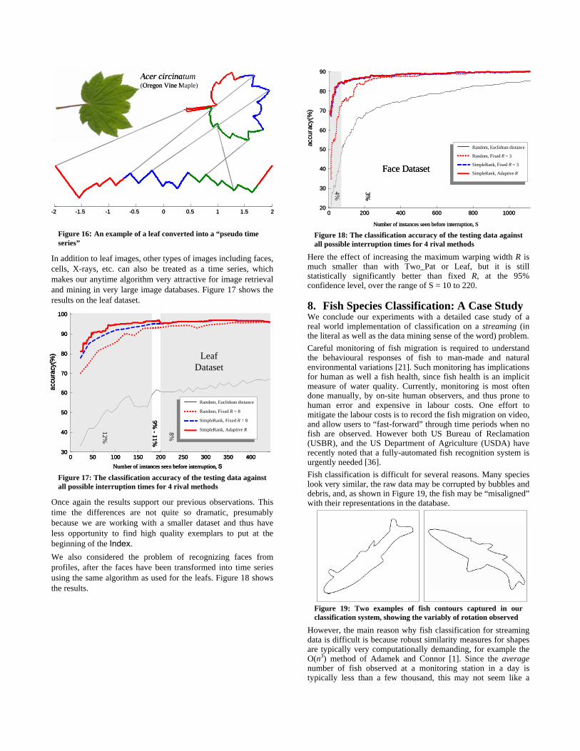
The results are very encouraging; our method allows us to obtain near perfect accuracy after seeing only a tiny fraction of the instances. Note that this experiment strongly supports our observations in Section 6.2, which states that the best value of R is inversely related to database size. The Leaf dataset consists of 442 leaf images, from four species of Maple and two species of Oak trees. It has been shown that an image can be converted into a “pseudo time series” [26]. Here, we have converted each leaf image to a time series by measuring the local curvature along its outline. Figure 16 shows a maple leaf image and its times series representation.

0 200 400 600 800 100020

30

40

50

60

70

80

90


accu

racy

(%)

Face Dataset


Random, Fixed R = 4




Random, Fixed R = 3



3%4%

0 200 400 600 800 100020

30

40

50

60

70

80

90


accu

racy

(%)

Face Dataset


Random, Fixed R = 4




Random, Fixed R = 3



3%4%

Acer circinatum(Oregon Vine Maple)

-2 -1.5 -1 -0.5 0 0.5 1 1.5 2

Acer circinatum(Oregon Vine Maple)

-2 -1.5 -1 -0.5 0 0.5 1 1.5 2

Figure 16: An example of a leaf converted into a “pseudo time series”

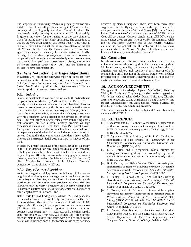
In addition to leaf images, other types of images including faces, cells, X-rays, etc. can also be treated as a time series, which makes our anytime algorithm very attractive for image retrieval and mining in very large image databases. Figure 17 shows the results on the leaf dataset.

Figure 17: The classification accuracy of the testing data against all possible interruption times for 4 rival methods

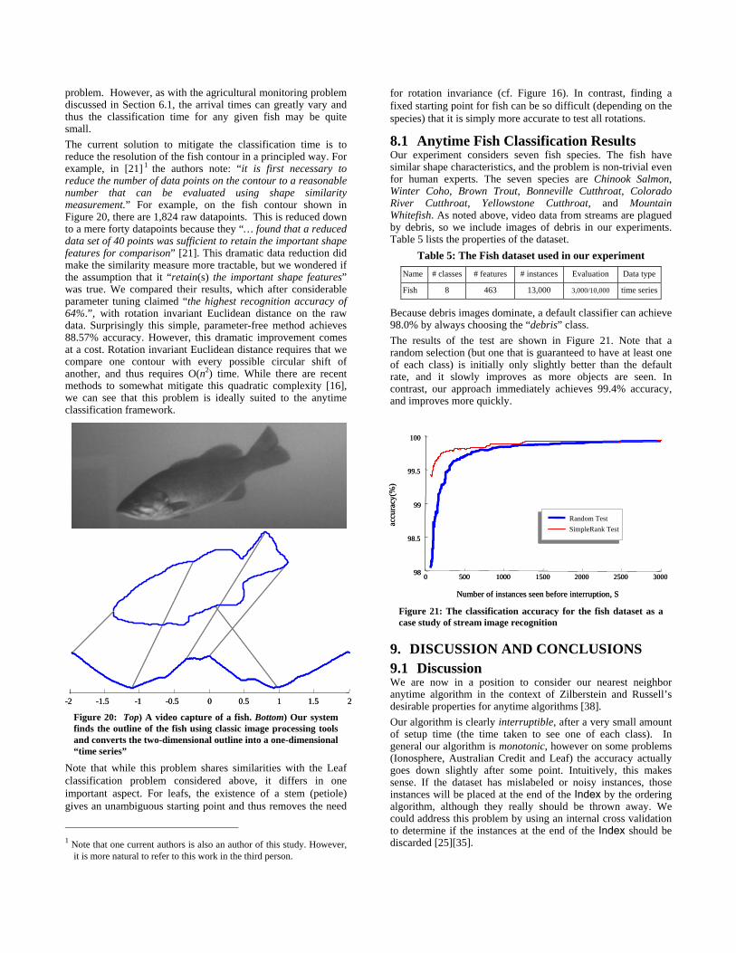
Once again the results support our previous observations. This time the differences are not quite so dramatic, presumably because we are working with a smaller dataset and thus have less opportunity to find high quality exemplars to put at the beginning of the Index. We also considered the problem of recognizing faces from profiles, after the faces have been transformed into time series using the same algorithm as used for the leafs. Figure 18 shows the results.

Figure 18: The classification accuracy of the testing data against all possible interruption times for 4 rival methods

Here the effect of increasing the maximum warping width R is much smaller than with Two_Pat or Leaf, but it is still statistically significantly better than fixed R, at the 95% confidence level, over the range of S = 10 to 220.

8. Fish Species Classification: A Case Study We conclude our experiments with a detailed case study of a real world implementation of classification on a streaming (in the literal as well as the data mining sense of the word) problem.

0 50 100 150 200 250 300 350 40030

40

50

60

70

80

90

100

accu

racy

(%)

8%

9% -11%

12%


Random, Fixed R = 8




Leaf Dataset

0 50 100 150 200 250 300 350 40030

40

50

60

70

80

90

100

accu

racy

(%)

8%

9% -11%

12%


Random, Fixed R = 8




0 50 100 150 200 250 300 350 40030

40

50

60

70

80

90

100

accu

racy

(%)

8%

9% -11%

12%


Random, Fixed R = 8




Random, Fixed R = 8




Leaf Dataset

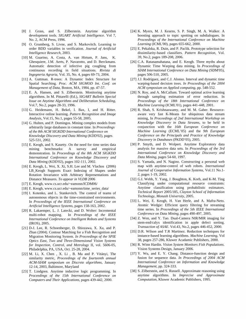
Careful monitoring of fish migration is required to understand the behavioural responses of fish to man-made and natural environmental variations [21]. Such monitoring has implications for human as well a fish health, since fish health is an implicit measure of water quality. Currently, monitoring is most often done manually, by on-site human observers, and thus prone to human error and expensive in labour costs. One effort to mitigate the labour costs is to record the fish migration on video, and allow users to “fast-forward” through time periods when no fish are observed. However both US Bureau of Reclamation (USBR), and the US Department of Agriculture (USDA) have recently noted that a fully-automated fish recognition system is urgently needed [36]. Fish classification is difficult for several reasons. Many species look very similar, the raw data may be corrupted by bubbles and debris, and, as shown in Figure 19, the fish may be “misaligned” with their representations in the database.

Figure 19: Two examples of fish contours captured in our classification system, showing the variably of rotation observed

However, the main reason why fish classification for streaming data is difficult is because robust similarity measures for shapes are typically very computationally demanding, for example the O(n3) method of Adamek and Connor [1]. Since the average number of fish observed at a monitoring station in a day is typically less than a few thousand, this may not seem like a

problem. However, as with the agricultural monitoring problem discussed in Section 6.1, the arrival times can greatly vary and thus the classification time for any given fish may be quite small. The current solution to mitigate the classification time is to reduce the resolution of the fish contour in a principled way. For example, in [21] 1 the authors note: “it is first necessary to reduce the number of data points on the contour to a reasonable number that can be evaluated using shape similarity measurement.” For example, on the fish contour shown in Figure 20, there are 1,824 raw datapoints. This is reduced down to a mere forty datapoints because they “… found that a reduced data set of 40 points was sufficient to retain the important shape features for comparison” [21]. This dramatic data reduction did make the similarity measure more tractable, but we wondered if the assumption that it “retain(s) the important shape features” was true. We compared their results, which after considerable parameter tuning claimed “the highest recognition accuracy of 64%.”, with rotation invariant Euclidean distance on the raw data. Surprisingly this simple, parameter-free method achieves 88.57% accuracy. However, this dramatic improvement comes at a cost. Rotation invariant Euclidean distance requires that we compare one contour with every possible circular shift of another, and thus requires O(n2) time. While there are recent methods to somewhat mitigate this quadratic complexity [16], we can see that this problem is ideally suited to the anytime classification framework.

Figure 20: Top) A video capture of a fish. Bottom) Our system finds the outline of the fish using classic image processing tools and converts the two-dimensional outline into a one-dimensional “time series”

Note that while this problem shares similarities with the Leaf classification problem considered above, it differs in one important aspect. For leafs, the existence of a stem (petiole) gives an unambiguous starting point and thus removes the need

1 Note that one current authors is also an author of this study. However,

it is more natural to refer to this work in the third person.

for rotation invariance (cf. Figure 16). In contrast, finding a fixed starting point for fish can be so difficult (depending on the species) that it is simply more accurate to test all rotations.

8.1 Anytime Fish Classification Results Our experiment considers seven fish species. The fish have similar shape characteristics, and the problem is non-trivial even for human experts. The seven species are Chinook Salmon, Winter Coho, Brown Trout, Bonneville Cutthroat, Colorado River Cutthroat, Yellowstone Cutthroat, and Mountain Whitefish. As noted above, video data from streams are plagued by debris, so we include images of debris in our experiments. Table 5 lists the properties of the dataset.

Table 5: The Fish dataset used in our experiment Name # classes # features # instances Evaluation Data type

Fish 8 463 13,000 3,000/10,000 time series

Because debris images dominate, a default classifier can achieve 98.0% by always choosing the “debris” class. The results of the test are shown in Figure 21. Note that a random selection (but one that is guaranteed to have at least one of each class) is initially only slightly better than the default rate, and it slowly improves as more objects are seen. In contrast, our approach immediately achieves 99.4% accuracy, and improves more quickly.

-2 -1.5 -1 -0.5 0 0.5 1 1.5 2-2 -1.5 -1 -0.5 0 0.5 1 1.5 2

0 500 1000 1500 2000 2500 300098

98.5

99

99.5

100


accu

racy

(%)

Random TestSimpleRank Test

0 500 1000 1500 2000 2500 300098

98.5

99

99.5

100


accu

racy

(%)

Random TestSimpleRank Test

Figure 21: The classification accuracy for the fish dataset as a case study of stream image recognition

9. DISCUSSION AND CONCLUSIONS 9.1 Discussion We are now in a position to consider our nearest neighbor anytime algorithm in the context of Zilberstein and Russell’s desirable properties for anytime algorithms [38]. Our algorithm is clearly interruptible, after a very small amount of setup time (the time taken to see one of each class). In general our algorithm is monotonic, however on some problems (Ionosphere, Australian Credit and Leaf) the accuracy actually goes down slightly after some point. Intuitively, this makes sense. If the dataset has mislabeled or noisy instances, those instances will be placed at the end of the Index by the ordering algorithm, although they really should be thrown away. We could address this problem by using an internal cross validation to determine if the instances at the end of the Index should be discarded [25][35].

The property of diminishing returns is generally dramatically satisfied. For almost all problems, we get 90% of the final accuracy after seeing only the first 10% of the data. The measurable quality property is a little more difficult to satisfy. In general the curves for the training error are very similar to those for testing error, but slightly optimistic. The exceptions to this are the very small datasets, and Forest Cover Type, which is known to have a training set that is unrepresentative of the test set. We can therefore use the training error curves to obtain approximate expected accuracy for unseen instances. Finally, our algorithm is clearly preemptable. If we wish to stop it temporarily and restart it later, we need only save three numbers, the current class prediction (best_match_class), the current best-so-far distance (best_match_val), and the number of objects we have seen thusfar (p).

9.2 Why Not Indexing or Eager Algorithms? In Section 2 we posed the following rhetorical questions from an imagined critic of our work; “why not use an indexing technique to speed up nearest neighbor?”, and “why not use a faster classification algorithm like a decision tree?.” We are now in a position to answer these questions.

9.2.1 Indexing Given the constraints of our problem we could theoretically use a Spatial Access Method (SAM) such as an R-tree [11] to quickly locate the nearest neighbor for our classifier. However there are several reasons why this is not a solution to the task at hand. In the best case, index trees require O(log2m) time to locate the nearest neighbor, however this O(log2m) comes with very high constants (which depend on the dimensionality of the data). The real utility of SAMs comes from minimizing costly disk accesses, but for a main memory problem on high dimensional data (as in Leaf, Face, Two_Pat, Forest Cover, Ionosphere etc) we are able to do a fast linear scan and see a large percentage of the data before the index structure returns an answer. During this time our anytime algorithm is interruptible, whereas an interrupted SAM does not have an answer of any kind. In addition, a major advantage of the nearest neighbor algorithm is that it is defined for any similarity/dissimilarity measure, including measures that either cannot be indexed, or are indexed only with great difficulty. For example, string, graph or tree edit distance, rotation invariant Euclidean distance (cf. Section 8) [16], Mahalanobis distance, Earth Movers Distance, compression based similarity [22] etc.

9.2.2 Eager Learner Algorithms As to the suggestion of bypassing the lethargy of the nearest neighbor algorithm by using an eager learner such as a decision tree or Bayesian classifier, we can address this idea with a single word: accuracy. There exist many problems for which the best-known classifier is Nearest Neighbor. As a concrete example, let us consider just time series classification, which we discussed at some length above in Sections 6 and 8. Both Geurts [7] and Rodriguez & Alonso [27], independently introduced decision trees to classify time series. On the Two Patterns dataset, they report error rates of 4.84% and 4.90% respectively. However, in our experiments on the same dataset (cf. Figure 15) our anytime algorithm achieves the same accuracy after seeing only 47 instances, and thereafter rapidly converges on a 0.0% error rate. While there have been several other attempts to classify time series with decision trees, to the best of our knowledge none of them comes close to the accuracy

achieved by Nearest Neighbor. There have been many other suggestions for classifying time series with eager learners. For example, in a recent work Wu and Chang [37], use a “super-kernel fusion scheme” to achieve accuracy of 0.79% on the ControlChart dataset. However simply using 1NN-DTW on the same dataset gives an error rate of 0.33%. In summary, while the “no free lunch” theorem tells us that Nearest Neighbor classifier is not optimal for all problems, there are many problems where the Nearest Neighbor classifier is the best-known solution in spite of decades of research.

9.3 Conclusion In this work we have shown a simple method to convert the ubiquitous nearest neighbor algorithm into an anytime algorithm. We have shown, on a highly diverse set of problems, that our algorithm can achieve high accuracy even if interrupted after seeing only a small fraction of the dataset. Future work includes investigation of other ordering algorithms and a field study of anytime classification for insect classification [33].

10. ACKNOWLEDGMENTS We gratefully acknowledge Agenor Mafra-Neto, Geoffrey Webb, Jill Brady and Ying Yang for their useful suggestions. We further wish to acknowledge Dennis Shiozawa, Xiaoqian Xua, and Pengcheng Zhana at Brigham Young University, and Robert Schoenberger with Agris-Schoen Vision Systems for their help with the fish monitoring problem. This research was partly funded by the National Science Foundation under grant IIS-0237918.

11. REFERENCES [1] T. Adamek, and N. E. Connor. A multiscale representation

method for nonrigid shapes with a single closed contour. IEEE Circuits and Systems for Video Technology, Vol.14, pages 742- 753, 2004.

[2] C. Aggarwal, J. Han, J. Wang, and P. S. Yu. On demand classification of data streams. In Proceedings of the International Conference on Knowledge Discovery and Data Mining (KDD'04), 2004.

[3] J. L. Bentley, and R. Sedgewick. Fast algorithms for sorting and searching strings. In Proceedings of the 8th Annual ACM-SIAM Symposium on Discrete Algorithms, pages 360-369, 1997.

[4] H. I. Bozma, and Hulya Yalcin. Visual processing and classification of items on a moving conveyor: A selective perception approach. Robotics and Computer Integrated Manufacturing, Vol.18, No.2, pages 125-133, 2002.

[5] P. Bradley, U. Fayyad and C. Reina. Scaling clustering algorithms to large databases. In Proceedings of the 4th International Conference on Knowledge Discovery and Data Mining (KDD'98), pages 9-15, 1998.

[6] S. Esmeir, and S. Markovitch. Interruptible anytime algorithms for iterative improvement of decision trees. In Proceedings of Workshop on the Utility-Based Data Mining (UBDM-2005), held with The 11th ACM SIGKDD International Conference on Knowledge Discovery and Data Mining (KDD'05), 2005.

[7] P. Geurts. Contributions to decision tree induction: bias/variance tradeoff and time series classification. Ph.D. thesis, Department of Electrical Engineering and Computer Science, University of Liege, Belgium, 2002.

[8] J. Grass, and S. Zilberstein. Anytime algorithm development tools. SIGART Artificial Intelligence. Vol 7, No. 2, ACM Press, 1996.

[9] O. Grumberg, S. Livne, and S. Markovitch. Learning to order BDD variables in verification. Journal of Artificial Intelligence Research, 2003.

[10] M. Guarino, A. Costa, A. van Hirtum, P. Jans, K. Ghesquiere, J.M. Aerts, P. Navarotto, and D. Berckmans. Automatic detection of infective pig coughing from continuous recording in field situations. Rivista di Ingegneria Agraria, Vol. 35, No. 4, pages 69-73, 2004.

[11] A. Guttman. R-trees: A Dynamic Index Structure for Spatial Searching. Proc. ACM SIGMOD Int. Conf. on Management of Data, Boston, MA, 1984, pp. 47-57.

[12] E. A. Hansen, and S. Zilberstein. Monitoring anytime algorithms. In M. Pittarelli (Ed.), SIGART Bulletin Special Issue on Anytime Algorithms and Deliberation Scheduling, Vol.7, No.2, pages 28-33, 1996.

[13] G. Heidemann, H. Bekel, I. Bax, I, and H. Ritter. Interactive online learning. Pattern Recognition and Image Analysis, Vol.15, No.1, pages 55-58, 2005.

[14] G. Hulten, and P. Domingos. Mining complex models from arbitrarily large databases in constant time. In Proceedings of the 8th ACM SIGKDD International Conference on Knowledge Discovery and Data Mining (KDD'02), pages 525-531, 2002.

[15] E. Keogh, and S. Kasetty. On the need for time series data mining benchmarks: A survey and empirical demonstration. In Proceedings of the 8th ACM SIGKDD International Conference on Knowledge Discovery and Data Mining (KDD'02), pages 102-111, 2002.

[16] E. Keogh, L. Wei, X. Xi, S.H. Lee and M. Vlachos (2006) LB_Keogh Supports Exact Indexing of Shapes under Rotation Invariance with Arbitrary Representations and Distance Measures. To appear in VLDB 2006

[17] E. Keogh, www.cs.ucr.edu/~eamonn/ICDM06/ [18] E. Keogh, www.cs.ucr.edu/~eamonn/time_series_data/ [19] I. Kotenko, and L. Stankevitch. The control of teams of

autonomous objects in the time-constrained environments. In Proceedings of the IEEE International Conference on Artificial Intelligence Systems, pages 158-163, 2002.

[20] R. Lakaemper, L. J. Latecki, and D. Wolter: Incremental multi-robot mapping. In Proceedings of the IEEE International Conference on Intelligent Robots and Systems (IROS), 2005.

[21] D-J. Lee, R. Schoenberger, D. Shiozawa, X. Xu, and P. Zhan (2004). Contour Matching for a Fish Recognition and Migration Monitoring System. In Proceedings of the SPIE Optics East, Two and Three-Dimensional Vision Systems for Inspection, Control, and Metrology II, vol. 5606-05, Philadelphia, PA, USA, Oct. 25-28, 2004.

[22] M. Li, X. Chen , X. Li , B. Ma and P. Vitányi, The similarity metric, Proceedings of the fourteenth annual ACM-SIAM symposium on Discrete algorithms, January 12-14, 2003, Baltimore, Maryland

[23] T. Lindgren. Anytime inductive logic programming. In Proceedings of the 15th International Conference on Computers and Their Applications, pages 439-442, 2000.

[24] K. Myers, M. J. Kearns, S. P. Singh, M. A. Walker. A boosting approach to topic spotting on subdialogues. In Proceedings of the International Conference on Machine Learning (ICML'00), pages 655-662, 2000.

[25] E. Pekalska, R. Duin, and P. Paclik. Prototype selection for dissimilarity-based classifiers. Pattern Recognition, Vol. 39, No.2, pages 189-208, 2006.

[26] C.A. Ratanamahatana, and E. Keogh. Three myths about Dynamic Time Warping data mining. In Proceedings of SIAM International Conference on Data Mining (SDM'05), pages 506-510, 2005.

[27] J.J. Rodríguez, and C.J. Alonso. Interval and dynamic time warping-based decision trees. In Proceedings of the 2004 ACM symposium on Applied computing, pp. 548-552.

[28] N. Roy, and A. McCallum. Toward optimal active learning through sampling estimation of error reduction. In Proceedings of the 18th International Conference on Machine Learning (ICML'01), pages 441-448, 2001.

[29] R. Shah, S. Krishnaswamy, and M. M. Gaber. Resource-aware very fast K-Means for ubiquitous data stream mining, In Proceedings of 2nd International Workshop on Knowledge Discovery in Data Streams, to be held in conjunction with the 16th European Conference on Machine Learning (ECML’05) and the 9th European Conference on the Principals and Practice of Knowledge Discovery in Databases (PKDD’05), 2005.

[30] P. Smyth, and D. Wolpert. Anytime Exploratory data analysis for massive data sets. In Proceedings of the 3rd International Conference on Knowledge Discovery and Data Mining, pages 54-60, 1997.

[31] S. Yamada, and N. Nagino. Constructing a personal web map with anytime-control of web robots. International Journal of Cooperative Information Systems, Vol.11 No.1-2, pages 1-19, 2002.

[32] G.I. Webb, Y. Yang, J. Boughton, K. Korb, and K-M. Ting Classifying under computational resource constraints: Anytime classification using probabilistic estimators. Technical Report 2005/185, Clayton School of Information Technology, Monash University, 2005.

[33] L. Wei, E. Keogh, H. Van Herle, and A. Mafra-Neto. Atomic Wedgie: Efficient query filtering for streaming time series. In Proceedings of the 5th IEEE International Conference on Data Mining, pages 490-497, 2005.

[34] Z. Wen, and Y. Tao. Dual-Camera NIR/MIR imaging for stem-end/calyx identification in apple defect sorting. Transaction of ASAE. Vol.43, No.2, pages 446-452, 2000.

[35] D.R. Wilson and T.R Martinez. Reduction techniques for instance-based learning algorithms. Machine Learning, Vol 38, pages 257-286, Kluwer Acadamic Publishers, 2000.

[36] R. Winn Hardin. Vision System Monitors Fish Populations. Vision Systems Design, January 2006.

[37] Y. Wu, and E. Y. Chang. Distance-function design and fusion for sequence data. In Proceedings of 2004 ACM International Conference on Information and Knowledge Management, pp. 324-333.

[38] S. Zilberstein, and S. Russell. Approximate reasoning using anytime algorithms. In Imprecise and Approximate Computation, Kluwer Academic Publishers, 1995.

Anytime Classification Using the Nearest Neighbor …eamonn/Anytime_Classification.pdfAnytime...

Documents

Transcript of Anytime Classification Using the Nearest Neighbor …eamonn/Anytime_Classification.pdfAnytime...