
Antonio Acconcia, Giancarlo Corsetti and Saverio Simonelli. MAFIA AND PUBLIC SPENDING: EVIDENCE ON...
74
M AFIA AND P UBLIC S PENDING :E VIDENCE ON THE F ISCAL M ULTIPLIER FROM A Q UASI - EXPERIMENT Antonio Acconcia, Giancarlo Corsetti and Saverio Simonelli Bank of Estonia Tallin, August 19 2014 1 / 74
-
Upload
eesti-pank -
Category
Economy & Finance
-
view
110 -
download
1
Transcript of Antonio Acconcia, Giancarlo Corsetti and Saverio Simonelli. MAFIA AND PUBLIC SPENDING: EVIDENCE ON...

MAFIA AND PUBLIC SPENDING: EVIDENCE ON
THE FISCAL MULTIPLIER FROM A
QUASI-EXPERIMENT
Antonio Acconcia, Giancarlo Corsetti and Saverio Simonelli
Bank of Estonia
Tallin, August 19 2014
1 / 74

The main question
I Transmission of fiscal policy: How to recover ‘multipliereffects’?
I Focus of the debate: Identify innovations to spending or taxation,distinct from variations that are systematically related to thebusiness cycle.
I Reverse causation and anticipation effects may spuriously raise,or lower, estimated multipliers (see e.g. Barro and Redlick 2011and Ramey 2011).
I But suppose we can identify a truly exogenous shock. Itstransmission can be expected to be different across economic‘environments’, reflecting policy, strucutal and cyclical factors.
I A single estimate of ‘the’ multiplier cannot provide a goodguidance to policymaker in all circumstances.
2 / 74
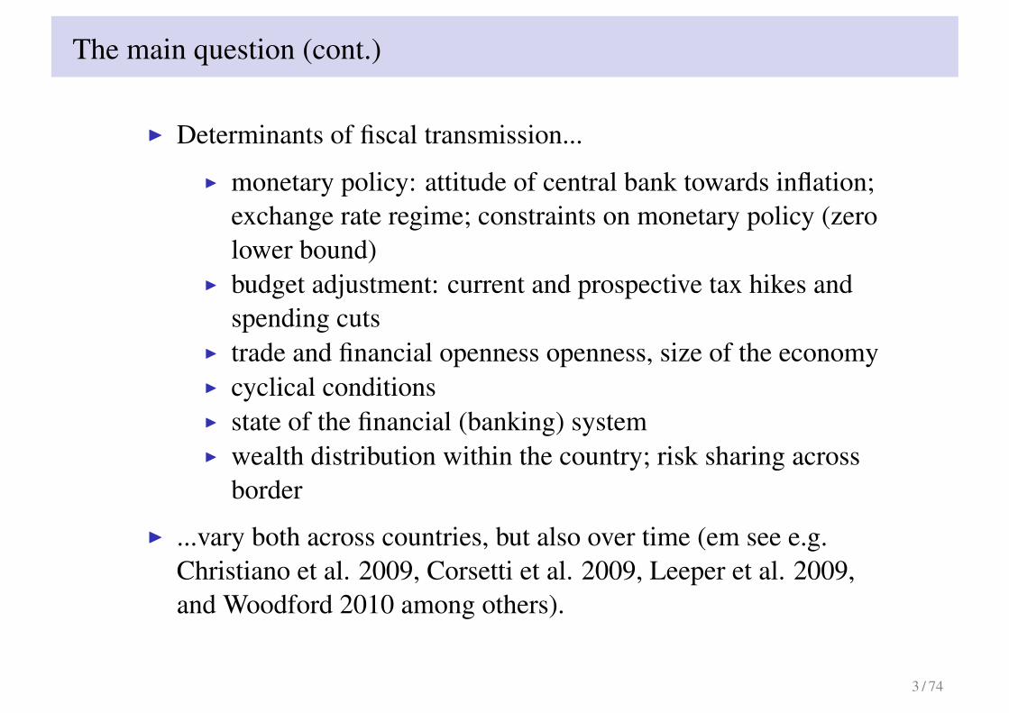
The main question (cont.)
I Determinants of fiscal transmission...
I monetary policy: attitude of central bank towards inflation;exchange rate regime; constraints on monetary policy (zerolower bound)
I budget adjustment: current and prospective tax hikes andspending cuts
I trade and financial openness openness, size of the economyI cyclical conditionsI state of the financial (banking) systemI wealth distribution within the country; risk sharing across
border
I ...vary both across countries, but also over time (em see e.g.Christiano et al. 2009, Corsetti et al. 2009, Leeper et al. 2009,and Woodford 2010 among others).
3 / 74

The main question (cont.)
I By way of example, the following theoretical example draws ona 2010 paper on the transmission of spending shock acrossexchange rate regimes joint with Keith Kuester and GernotMueller.
I To connect with the rest of the talk, I focus on the effect of acontraction in spending.
4 / 74

Model
I Standard new Keynesian small open-economy model
I Imperfectly competitive firms produce country specific varieties
I Pricing in producer currency, prices sticky
I Domestic consumption biased towards home goods
I Government spending falls on home goods
I Complete markets versus incomplete markets/limitedparticipation (a fraction of households (λ) are without access toasset market)
I Policies
I Monetary policy: interest rate feedback rule or peg
I Lump-sum taxes respond to spending and debt
5 / 74
The transmission mechanism in the New Keynesian NK framework
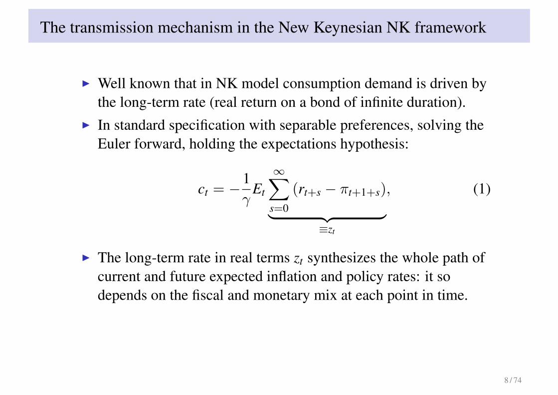
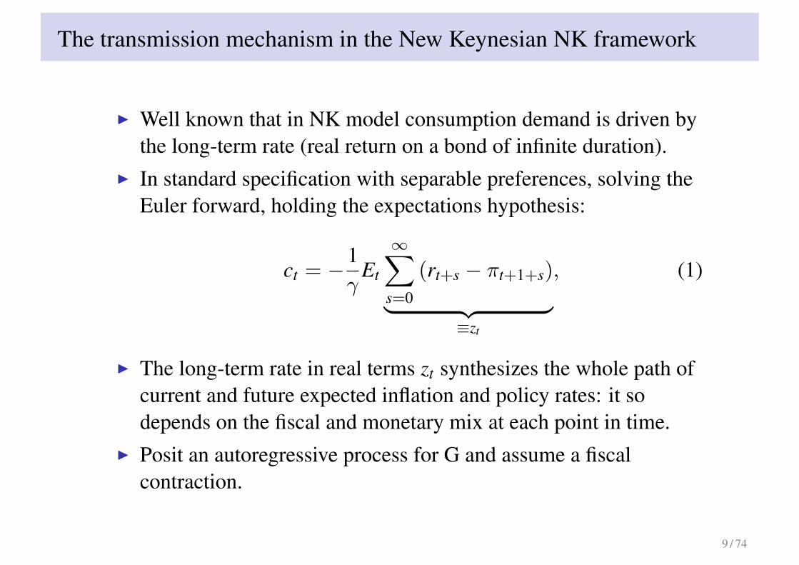
I Well known that in NK model consumption demand is driven bythe long-term rate (real return on a bond of infinite duration).
I In standard specification with separable preferences, solving theEuler forward, holding the expectations hypothesis:
ct = −1γ
Et
∞∑s=0
(rt+s − πt+1+s)︸ ︷︷ ︸≡zt
, (1)
I The long-term rate in real terms zt synthesizes the whole path ofcurrent and future expected inflation and policy rates: it sodepends on the fiscal and monetary mix at each point in time.
I Posit an autoregressive process for G and assume a fiscalcontraction.
6 / 74

The transmission mechanism in the New Keynesian NK framework
I Well known that in NK model consumption demand is driven bythe long-term rate (real return on a bond of infinite duration).
I In standard specification with separable preferences, solving theEuler forward, holding the expectations hypothesis:
ct = −1γ
Et
∞∑s=0
(rt+s − πt+1+s)︸ ︷︷ ︸≡zt
, (1)
I The long-term rate in real terms zt synthesizes the whole path ofcurrent and future expected inflation and policy rates: it sodepends on the fiscal and monetary mix at each point in time.
I Posit an autoregressive process for G and assume a fiscalcontraction.
7 / 74
The transmission mechanism in the New Keynesian NK framework
I Well known that in NK model consumption demand is driven bythe long-term rate (real return on a bond of infinite duration).
I In standard specification with separable preferences, solving theEuler forward, holding the expectations hypothesis:
ct = −1γ
Et
∞∑s=0
(rt+s − πt+1+s)︸ ︷︷ ︸≡zt
, (1)
I The long-term rate in real terms zt synthesizes the whole path ofcurrent and future expected inflation and policy rates: it sodepends on the fiscal and monetary mix at each point in time.
I Posit an autoregressive process for G and assume a fiscalcontraction.
8 / 74
The transmission mechanism in the New Keynesian NK framework
I Well known that in NK model consumption demand is driven bythe long-term rate (real return on a bond of infinite duration).
I In standard specification with separable preferences, solving theEuler forward, holding the expectations hypothesis:
ct = −1γ
Et
∞∑s=0
(rt+s − πt+1+s)︸ ︷︷ ︸≡zt
, (1)
I The long-term rate in real terms zt synthesizes the whole path ofcurrent and future expected inflation and policy rates: it sodepends on the fiscal and monetary mix at each point in time.
I Posit an autoregressive process for G and assume a fiscalcontraction.
9 / 74

The transmission mechanism in the New Keynesian NK framework
I Under Taylor rule and floating rates, negative inflation and policyrates throughout the relevant horizon cause a negative responsein long-term real rates, driving a positive consumption responseby agents who participate in the financial markets. Despite 30percent of population is hand-to-mouth consumers, the outputresponse is small.
I Taylor coefficient matters quantitatively though => degree ofmonetary accommodation (not shown).
10 / 74

Transmission of spending contraction under floating exchange rates
0 10 20 30−1.5
−1
−0.5
0
Government spending
limited
no limited
0 10 20 30−1
−0.5
0
Output
0 10 20 30−0.1
0
0.1
0.2
0.3
Private consumption
0 10 20 30−0.04
−0.03
−0.02
−0.01
0
Real interest rate (short)
0 10 20 30−0.4
−0.2
0
0.2
0.4
Real interest rate (long)
0 10 20 30−0.1
−0.05
0
Inflation
11 / 74
What about under a peg? A key analytical characterization
I Under a peg, by PPP lim t→∞ Pt = P∗, implying∑∞
t=0 πt = 0.
I Given the exchange rate constraint on the nominal short-termrate, the initial response of the real long-term rate is:
z0 =
( ∞∑t=0
−πt+1
)− π0︸ ︷︷ ︸
=0
+π0 = π0. (2)
I In response to stationary shocks, by PPP, a credible currencyunion (peg) means that any positive inflation today needs to becompensated by negative inflation tomorrow.
I This constrains the impact response of the real long-term interestrate to be equal to the initial, unanticipated, change in the CPI.
I Note: PPP needs to hold in the medium to the long run.
12 / 74
What about under a peg? A key analytical characterization (cont.)
I To the extent that initial inflation is small, so is the response ofconsumption of unconstrained agents.
I If only unconstrained agents, output than falls one to onewith the spending contraction.
I The multiplier is magnified by the response of hand-to-mouthconsumer.
13 / 74

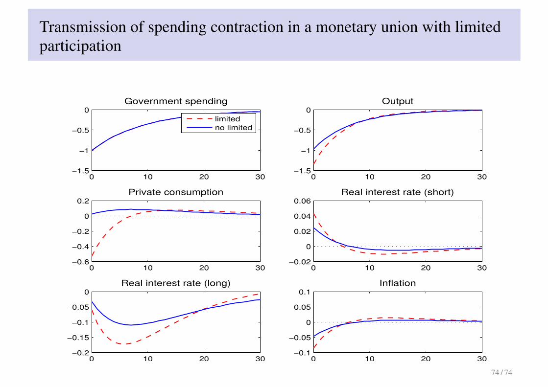
Transmission of spending contraction in a monetary union with limitedparticipation
0 10 20 30−1.5
−1
−0.5
0
Government spending
limited
no limited
0 10 20 30−1.5
−1
−0.5
0
Output
0 10 20 30−0.6
−0.4
−0.2
0
0.2
Private consumption
0 10 20 30−0.02
0
0.02
0.04
0.06
Real interest rate (short)
0 10 20 30−0.2
−0.15
−0.1
−0.05
0
Real interest rate (long)
0 10 20 30−0.1
−0.05
0
0.05
0.1
Inflation
14 / 74
A resolution to the ’Walters critique’
I As seen above, under a credible peg, long-term real rates mustincrease (and consumption fall) with impact inflation.
I This is so, even if short-term real rates move the other wayaround.
I In its well known critique of common currencies, Sir Waltersclaims that a peg is destabilizing, because an increase in inflationlowers real interest rates.
I He simply assume that short- and long-rates move together,which cannot be true in a credible monetary union.
I By the dynamic of inflation, negative real rates in the short runare followed by positive rates in the medium run (all indeviations from steady state).
I In our experiment, negative and positive rates offset each other asregards their effects on the long-term real rate on impact.
15 / 74

A resolution to the ’Walters critique’
I As seen above, under a credible peg, long-term real rates mustincrease (and consumption fall) with impact inflation.
I This is so, even if short-term real rates move the other wayaround.
I In its well known critique of common currencies, Sir Waltersclaims that a peg is destabilizing, because an increase in inflationlowers real interest rates.
I He simply assume that short- and long-rates move together,which cannot be true in a credible monetary union.
I By the dynamic of inflation, negative real rates in the short runare followed by positive rates in the medium run (all indeviations from steady state).
I In our experiment, negative and positive rates offset each other asregards their effects on the long-term real rate on impact.
16 / 74

A resolution to the ’Walters critique’
I As seen above, under a credible peg, long-term real rates mustincrease (and consumption fall) with impact inflation.
I This is so, even if short-term real rates move the other wayaround.
I In its well known critique of common currencies, Sir Waltersclaims that a peg is destabilizing, because an increase in inflationlowers real interest rates.
I He simply assume that short- and long-rates move together,which cannot be true in a credible monetary union.
I By the dynamic of inflation, negative real rates in the short runare followed by positive rates in the medium run (all indeviations from steady state).
I In our experiment, negative and positive rates offset each other asregards their effects on the long-term real rate on impact.
17 / 74

A resolution to the ’Walters critique’
I As seen above, under a credible peg, long-term real rates mustincrease (and consumption fall) with impact inflation.
I This is so, even if short-term real rates move the other wayaround.
I In its well known critique of common currencies, Sir Waltersclaims that a peg is destabilizing, because an increase in inflationlowers real interest rates.
I He simply assume that short- and long-rates move together,which cannot be true in a credible monetary union.
I By the dynamic of inflation, negative real rates in the short runare followed by positive rates in the medium run (all indeviations from steady state).
I In our experiment, negative and positive rates offset each other asregards their effects on the long-term real rate on impact.
18 / 74

A resolution to the ’Walters critique’
I As seen above, under a credible peg, long-term real rates mustincrease (and consumption fall) with impact inflation.
I This is so, even if short-term real rates move the other wayaround.
I In its well known critique of common currencies, Sir Waltersclaims that a peg is destabilizing, because an increase in inflationlowers real interest rates.
I He simply assume that short- and long-rates move together,which cannot be true in a credible monetary union.
I By the dynamic of inflation, negative real rates in the short runare followed by positive rates in the medium run (all indeviations from steady state).
I In our experiment, negative and positive rates offset each other asregards their effects on the long-term real rate on impact.
19 / 74

A resolution to the ’Walters critique’
I As seen above, under a credible peg, long-term real rates mustincrease (and consumption fall) with impact inflation.
I This is so, even if short-term real rates move the other wayaround.
I In its well known critique of common currencies, Sir Waltersclaims that a peg is destabilizing, because an increase in inflationlowers real interest rates.
I He simply assume that short- and long-rates move together,which cannot be true in a credible monetary union.
I By the dynamic of inflation, negative real rates in the short runare followed by positive rates in the medium run (all indeviations from steady state).
I In our experiment, negative and positive rates offset each other asregards their effects on the long-term real rate on impact.
20 / 74

Take home for the rest of the talk
I In a standard NK model of a small open economy in a currencyunion (a credible fixed exchange rate system), output multipliereffects are around 1 on impact.
I With limited participation, the impact multiplier is 1.3.I By the way, note that fiscal policy is effective under a float.
I This ends my example. Now, back to the main question.
21 / 74

Take home for the rest of the talk
I In a standard NK model of a small open economy in a currencyunion (a credible fixed exchange rate system), output multipliereffects are around 1 on impact.
I With limited participation, the impact multiplier is 1.3.
I By the way, note that fiscal policy is effective under a float.
I This ends my example. Now, back to the main question.
22 / 74

Take home for the rest of the talk
I In a standard NK model of a small open economy in a currencyunion (a credible fixed exchange rate system), output multipliereffects are around 1 on impact.
I With limited participation, the impact multiplier is 1.3.I By the way, note that fiscal policy is effective under a float.
I This ends my example. Now, back to the main question.
23 / 74

Take home for the rest of the talk
I In a standard NK model of a small open economy in a currencyunion (a credible fixed exchange rate system), output multipliereffects are around 1 on impact.
I With limited participation, the impact multiplier is 1.3.I By the way, note that fiscal policy is effective under a float.
I This ends my example. Now, back to the main question.
24 / 74

How to recover the multiplier?
How to recover “the multiplier”?
1. Identify innovations to spending or taxation, distinct fromvariations that are systematically related to the business cycle.
2. Control for determinants of transmission mechanism.
25 / 74

This paper
I We address both dimensions of empirical analyses of themultiplier by relying on a quasi-experiment setting usingsub-national data that enable us to:
1. identify temporary but sizeable variation in public spendingthat are exogenous to the cyclical conditions of theeconomy;
2. analyze their transmission controlling for monetary andbudget policy.
I Identification Strategy1. We instrument spending by exploiting an Italian law, which
causes sudden, large spending contractions unrelated to thecyclical economic conditions of the local economy.
2. We estimate the output multiplier of (large contractions in)public expenditure at provincial level in Italy, controllingfor both common cyclical movements and common policyimpulses at national level. By the characteristics of Italianfiscal federalism, the above temporary contractions havevirtually no effect on tax burden.
26 / 74

This paper
I We address both dimensions of empirical analyses of themultiplier by relying on a quasi-experiment setting usingsub-national data that enable us to:
1. identify temporary but sizeable variation in public spendingthat are exogenous to the cyclical conditions of theeconomy;
2. analyze their transmission controlling for monetary andbudget policy.
I Identification Strategy1. We instrument spending by exploiting an Italian law, which
causes sudden, large spending contractions unrelated to thecyclical economic conditions of the local economy.
2. We estimate the output multiplier of (large contractions in)public expenditure at provincial level in Italy, controllingfor both common cyclical movements and common policyimpulses at national level. By the characteristics of Italianfiscal federalism, the above temporary contractions havevirtually no effect on tax burden.
27 / 74
Preview of results
I Our point estimates suggest that, unless spending contractionsare compensated by monetary expansions or matched by lowertaxes, their effects on output are larger than the amount of thecut.
I Our IV estimate of the impact spending multiplier is 1.2,significantly larger than zero.
I Under the maintained hypothesis that lagged values of spendingare exogenous to current value added, dynamic effects raise ourpoint estimate to around 1.8.
I However, in our preferred model specification, we cannot rejectthe hypothesis that the multiplier is less than, or equal to one atstandard confidence levels.
I Fundamental insights on the transmission mechanism underlyingour results is provided by theoretical models already discussed.
28 / 74

Related evidence
I Together with the present study a number of works have recentlydelved into the analysis of multiplier effects using sub-nationaldata.
I Large multipliers, 1.5− 2, by Nakamura and Steinsson (2010),Serrato and Wingender (2010), Shoag (2010)
I Evidence, however, not supported by Clemens and Miran (2010)and Kraay (2011)
29 / 74
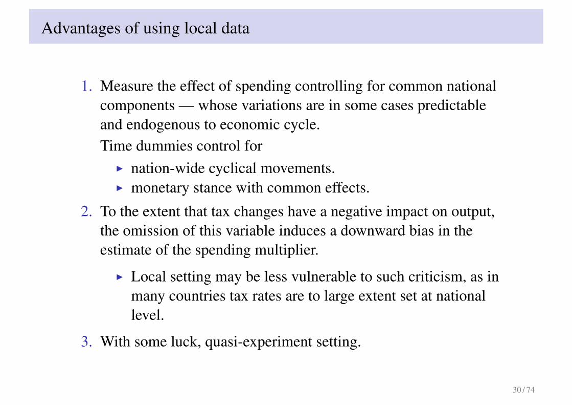
Advantages of using local data
1. Measure the effect of spending controlling for common nationalcomponents — whose variations are in some cases predictableand endogenous to economic cycle.Time dummies control for
I nation-wide cyclical movements.I monetary stance with common effects.
2. To the extent that tax changes have a negative impact on output,the omission of this variable induces a downward bias in theestimate of the spending multiplier.
I Local setting may be less vulnerable to such criticism, as inmany countries tax rates are to large extent set at nationallevel.
3. With some luck, quasi-experiment setting.
30 / 74

The empirical model
yi,t − yi,t−1
yi,t−1= αi + λt + β
gi,t − gi,t−1
yi,t−1+ γXi,t + vi,t
Yi,t = αi + λt + βGi,t + γXi,t + vi,t
where for each province i (95 Italian provincesX10 years=950observations).
I yi is per capita value added
I gi is the per capita infrastructure investment spending
I λt is a year fixed effectI αi is a province fixed effectI Xi,t denotes covariates (discussed below)
The coefficient β is the contemporaneous government spendingmultiplier.
31 / 74

Instrumenting Changes in Public Spending
I Despite advantages of using local information, OLS estimates ofthe multiplier subject to standard criticisms, e.g.
1. Spending on infrastructures is planned years before itactually takes place. A failure to account for anticipationeffects likely to bias results. (Ramey, 2009).
2. The government may systematically allocate funds inresponse to local developments, in ways that are notaccounted for by province-fixed effects.
I Need a good instrument for unexpected variations in publicspending exogenous to local economic conditions.
I We rely on a specific law by the Italian government, mandatingcompulsory administration of local municipalities on evidence ofmafia infiltration.
32 / 74

The institutional setting
I Italian penal code (articles 416-bis and 416-ter) recognizes thespecific nature of mafia crimes
I Specific to mafia is the use of intimidation, associative tiesand omerta’ (condition of silence), to acquire direct orindirect control of otherwise legal economic activities,especially in the area of provision of public services andpublic investment.
I To pursue their goals, Mafia-type associations have specificinterests in influencing the results of electoral competition,and obtain effective control over public tenders.
I Because of their sheer size of public works under the control oflocal administration, these have become one of the most lucrativebusinesses for mafia associations, generating profits comparableto those from extortions and selling drugs (see Relazione, 2000)
33 / 74
The institutional setting (cont.)
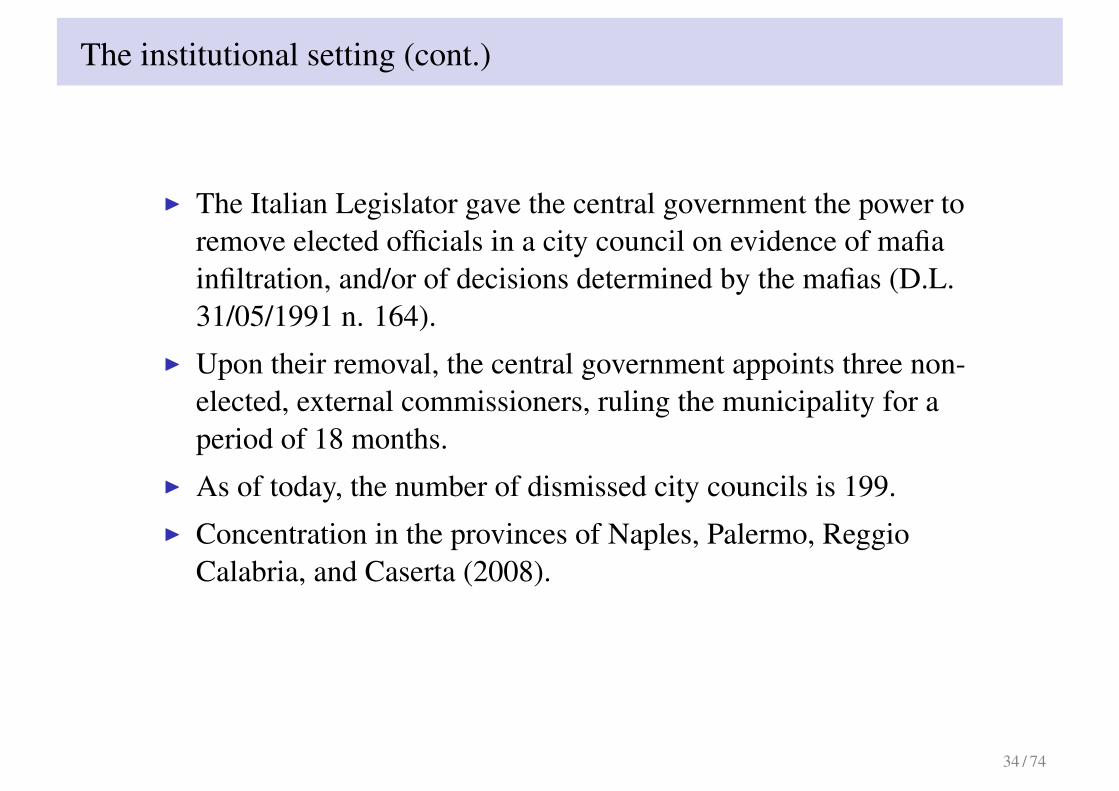
I The Italian Legislator gave the central government the power toremove elected officials in a city council on evidence of mafiainfiltration, and/or of decisions determined by the mafias (D.L.31/05/1991 n. 164).
I Upon their removal, the central government appoints three non-elected, external commissioners, ruling the municipality for aperiod of 18 months.
I As of today, the number of dismissed city councils is 199.I Concentration in the provinces of Naples, Palermo, Reggio
Calabria, and Caserta (2008).
34 / 74
The institutional setting (cont.)
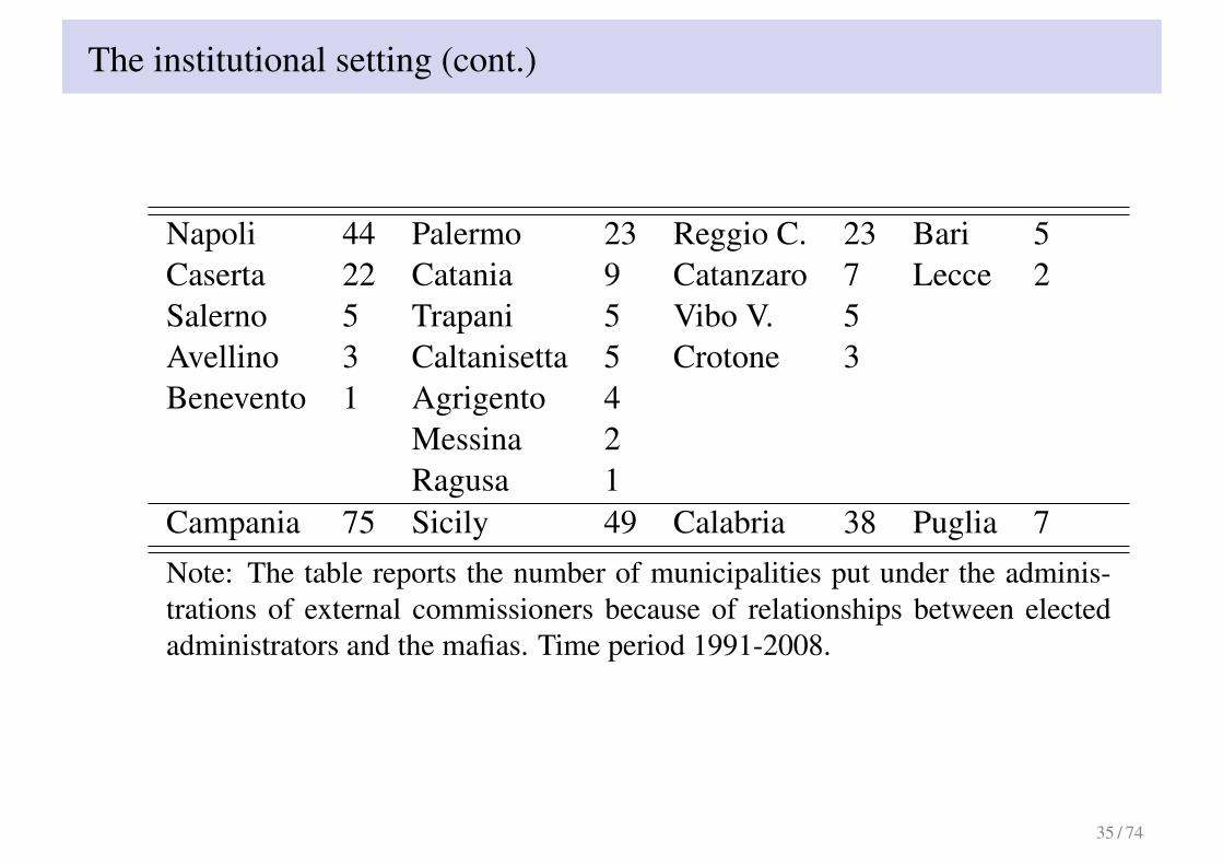
Napoli 44 Palermo 23 Reggio C. 23 Bari 5Caserta 22 Catania 9 Catanzaro 7 Lecce 2Salerno 5 Trapani 5 Vibo V. 5Avellino 3 Caltanisetta 5 Crotone 3Benevento 1 Agrigento 4
Messina 2Ragusa 1
Campania 75 Sicily 49 Calabria 38 Puglia 7Note: The table reports the number of municipalities put under the adminis-trations of external commissioners because of relationships between electedadministrators and the mafias. Time period 1991-2008.
35 / 74

An instrument "you can’t refuse"
I In our sample (1990-99), we have 109 cases of city councils putunder compulsory administrations. Aggregating them byprovince, we obtain 45 observations.
I The external administrators appointed by the central governmenthave the power to suspend financial flows into local public work.
I Public projects are started again only after investigation andscrutiny of previous tender procedures and decisions.
I The size of spending contractions is, on average, .5 percent ofvalue added.
36 / 74

Mean Difference Test
Log-difference Log-difference Percent of GDP Percent of GDPDifference -0.220*** -0.228** -0.555** -0.650*
[-3.63] [-3.21] [-2.61] [-2.45]Control group 0.0584*** 0.0666 0.120** 0.215
[4.70] [1.72] [3.10] [1.32]N 950 180 950 180
Note: The table shows results of mean difference tests relative to changes in publicinfrastructure investment. In the second and fourth columns of results we restrict toprovinces characterized by at least one case of local government dismission during theperiod analyzed. Data are annual from 1990 through 1999 at Italian province level. Thet-statistic is reported in brackets: *p < 0.05, **p < 0.01,***p < 0.001
37 / 74
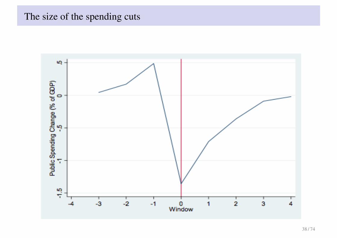
The size of the spending cuts
38 / 74

Randomness
I Is the instrument variation systematically related to localeconomic activity?
I The procedure leading to a dismissal of a city council because ofmafia infiltration is started by the prefetto on police reports onthe activities of the mafia in the municipality.
I The police evidence is produced in the course of investigationson crimes often unrelated to the control of local public work.
I Note that city council dismissals are not prompted byindicators of administrative inefficiency in the procurementprocedures.
I A check looking at growth pattern (relative to average) next.
39 / 74

Randomness (cont.)
Table: Randomness of council dismissals
> 0 < 0 > 0 or < 0t − 1 & t − 2 1/3 1/6 1/2t − 1 & t − 2 & t − 3 1/9 0 8/9Note: For two and three years before council dismissalshappened, the table reports the proportion of cases withprovincial growth rates always above the national average(column labeled with > 0), always below the nationalaverage (column labeled with < 0), without a constantsign (last column).
40 / 74

The instruments
I The first instrument (S1), equals the number of municipalitiesput under compulsory administration, provided that the officialdecree by which a city council is dismissed is formalized in thefirst semester of the year.
I The second instrument (S2) equals the number of municipalitiesput under compulsory administration in any given year, if theaverage number of days spent in such state is less than 180, andzero otherwise.
I In our baseline model, we instrument Gi,t entering S1contemporaneously and S2 lagged one period. Thus, the firststage regression of our baseline specification is
Gi,t = αi + λt + δ1S1i,t + δ2S2i,t−1 + γXi,t + ei,t
I The estimates of the coefficients of both instruments are alwaysnegative, as expected, and highly statistically significant.
41 / 74

Baseline Specification
I The presentation to follows progressively enlarges the set ofinstruments and controls.
I All regressions include:
I controls for unemployment (important differences acrossregions);
I controls for intensity of police investigations (more below).
42 / 74

Baseline Specification (cont.)
(1) (2) (3) (4)
G(t)1.17*
1.21* 1.29* 1.31*
[2.11] [2.30] [2.55] [2.54]
Y(t-1) -0.12 -0.13* -0.12
[-1.92] [-1.97] [-1.92]
Y(t-2) -0.01 -0.00 -0.00
[-0.11] [-0.07] [-0.07]
Council-dismissal(t-2) -0.30
[-1.73]
Council-dismissal(t-3) -0.08
[-0.49]
time effects YES YES YES YES
provincial fixed effects YES YES YES YES
controls for mafia investigation YES YES YES YES
unemployment rate proxies YES YES YES YES
number of instruments 2 2 2 4
First stage F-test 9.20 9.78 10.48 6.35
(p-value) (0.00) (0.00) (0.00) (0.00)
N 950 950 950 950
43 / 74

Baseline Specification (cont.)
I To address potential problems from serially correlated errors weinclude two lags of the left-hand-side variable among theregressors.
I Only the first lag is significant, but barely so.I The impact of adding these lags is negligible: there is hardly any
change in the point estimate and the significance of β.I The inclusion of the lagged dependent variable among the
regressors brings forward dynamic effects of the multiplier.I Net estimate is 1.14 (the ratio between the estimate of β and 1
minus the coefficient on Y (t − 1)).
44 / 74

Baseline Specification (cont.)
(1) (2) (3) (4)
G(t) 1.17*1.21* 1.29*
1.31*
[2.11] [2.30] [2.55] [2.54]
Y(t-1)-0.12 -0.13*
-0.12
[-1.92] [-1.97] [-1.92]
Y(t-2)-0.01 -0.00
-0.00
[-0.11] [-0.07] [-0.07]
Council-dismissal(t-2) -0.30
[-1.73]
Council-dismissal(t-3) -0.08
[-0.49]
time effects YES YES YES YES
provincial fixed effects YES YES YES YES
controls for mafia investigation YES YES YES YES
unemployment rate proxies YES YES YES YES
number of instruments 2 2 2 4
First stage F-test 9.20 9.78 10.48 6.35
(p-value) (0.00) (0.00) (0.00) (0.00)
N 950 950 950 950
45 / 74
Baseline Specification (cont.)
I We add as further controls two lags of “Council-dismissal”(att − 2 and t − 3) — recording the total number of municipalitiesput under compulsory administration by province × year
I The estimated coefficient for β is slightly higher relative to thespecification in the first column,
I However, the two lags of “Council-dismissal” are not statisticallysignificant .
46 / 74

Baseline Specification (cont.)
(1) (2) (3) (4)
G(t) 1.17* 1.21*1.29*
1.31*
[2.11] [2.30] [2.55] [2.54]
Y(t-1) -0.12 -0.13* -0.12
[-1.92] [-1.97] [-1.92]
Y(t-2) -0.01 -0.00 -0.00
[-0.11] [-0.07] [-0.07]
Council-dismissal(t-2)-0.30
[-1.73]
Council-dismissal(t-3)-0.08
[-0.49]
time effects YES YES YES YES
provincial fixed effects YES YES YES YES
controls for mafia investigation YES YES YES YES
unemployment rate proxies YES YES YES YES
number of instruments 2 2 2 4
First stage F-test 9.20 9.78 10.48 6.35
(p-value) (0.00) (0.00) (0.00) (0.00)
N 950 950 950 950
47 / 74

Baseline Specification (cont.)
I We now use the two lags of ‘council-dismissal’ (at t − 2 andt − 3) to enlarge the set of instruments, rather than as controls.
I Since the compulsory administration is designed to last 18months, it may have effects on three consecutive calendar years.
I Our estimate of the coefficient β is substantially unaffectedrelative to column (3).
I In our overidentified models, however, the first-stage F-statisticfor the model with 4 instruments halves in size.
I Note nonetheless that, as for the other regressions with 2instruments , the Hansen Jstatistic implies a p-value around 0.3,suggesting that the instruments are uncorrelated with the errorterm.
48 / 74

Baseline Specification (cont.)
(1) (2) (3) (4)
G(t) 1.17* 1.21* 1.29*1.31*
[2.11] [2.30] [2.55] [2.54]
Y(t-1) -0.12 -0.13* -0.12
[-1.92] [-1.97] [-1.92]
Y(t-2) -0.01 -0.00 -0.00
[-0.11] [-0.07] [-0.07]
Council-dismissal(t-2) -0.30
[-1.73]
Council-dismissal(t-3) -0.08
[-0.49]
time effects YES YES YES YES
provincial fixed effects YES YES YES YES
controls for mafia investigation YES YES YES YES
unemployment rate proxies YES YES YES YES
number of instruments 2 2 24
First stage F-test 9.20 9.78 10.48 6.35
(p-value) (0.00) (0.00) (0.00) (0.00)
N 950 950 950 950
49 / 74

Baseline Specification (cont.)
I Add two lags of public investment expenditure to our set ofcovariates.
I In both model specifications reported in the table, the coefficientof the first lag is statistically and economically significant, with apoint estimate which is about one half that of the impactcoefficient.
I Under the assumption that spending is predetermined to currentoutput, this effect should be added to our IV estimate of themultiplier.
50 / 74
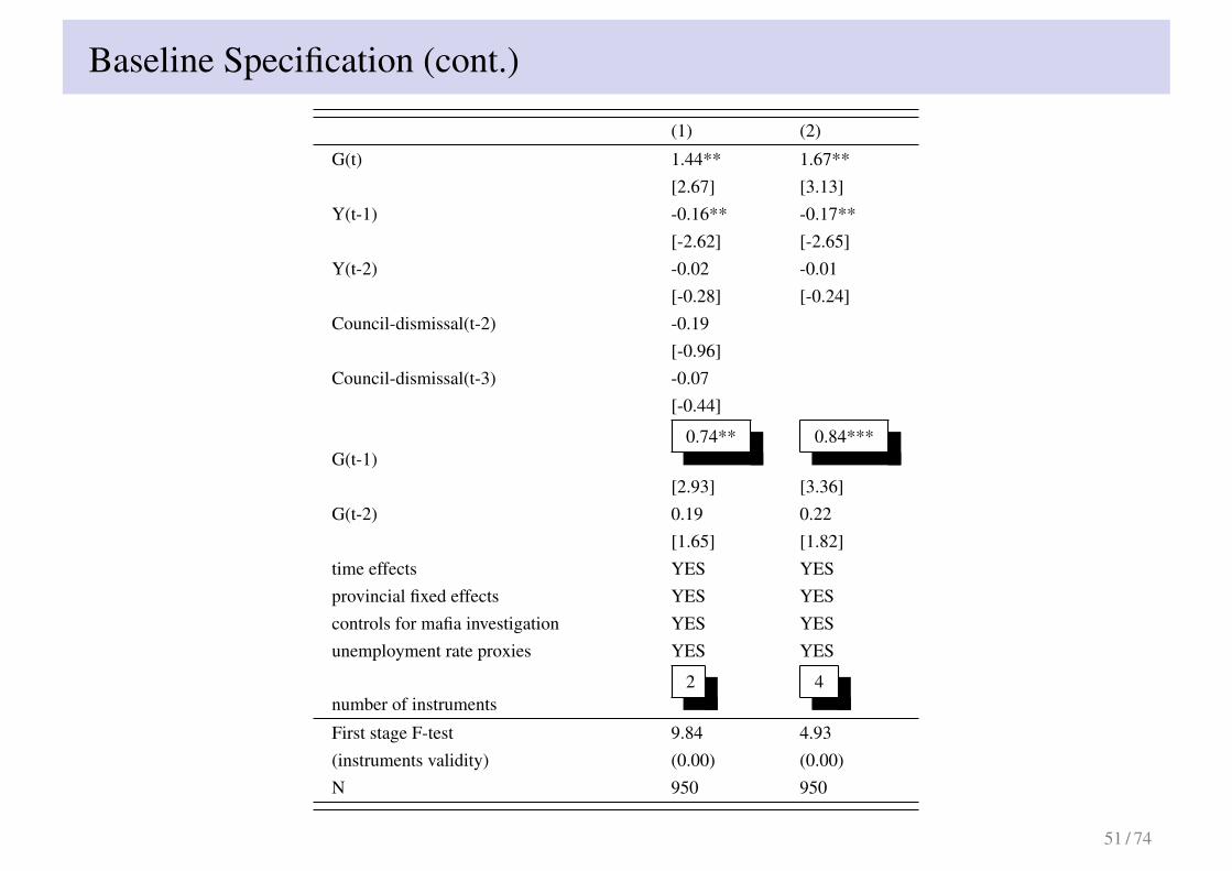
Baseline Specification (cont.)
(1) (2)
G(t) 1.44** 1.67**[2.67] [3.13]
Y(t-1) -0.16** -0.17**[-2.62] [-2.65]
Y(t-2) -0.02 -0.01[-0.28] [-0.24]
Council-dismissal(t-2) -0.19[-0.96]
Council-dismissal(t-3) -0.07[-0.44]
G(t-1)0.74** 0.84***
[2.93] [3.36]G(t-2) 0.19 0.22
[1.65] [1.82]time effects YES YESprovincial fixed effects YES YEScontrols for mafia investigation YES YESunemployment rate proxies YES YES
number of instruments2 4
First stage F-test 9.84 4.93(instruments validity) (0.00) (0.00)N 950 950
51 / 74

Baseline Specification (cont.)
I In our preferred specification (with 2 instrument), controlling formonetary and budget policy:
I the estimate of the net multiplier effect of Gt is 1.24I adding up this to the coefficients relative to the one-year
lagged spending changes, the point estimate of the overallmultiplier is as high as 1.87.
I Nonetheless, we are not able to reject the null hypothesisβ 6 1in favor of β > 1
I cannot exclude the possibility that the contraction in publicspending is marginally offset by a simultaneous increase inprivate demand.
52 / 74
The influence of individual provinces
I It is plausible that some episodes exerts a stronger influence onour estimates.
I We address this issue, by analyzing the extent to which ourresults are sensitive to the exclusion of any particular provincefrom the analysis.
I we report results for the most comprehensive specifications ofour model with 2 instruments, excluding one of the followingprovinces in turn: Napoli, Caserta, Palermo, Catania, Salerno,Bari, Reggio Calabria.
I None of these provinces is a crucial driver of our estimates.I The point estimates of β are in the range 1.26-1.50, while those
of coefficient of the lagged public spending ranges from 0.67 to0.77 (with the proportion between the two remaining roughlyconstant).
53 / 74

The influence of individual provinces (cont.)
NA CE PA CT SA BA RC
G(t) 1.50** 1.26* 1.40* 1.27* 1.40* 1.43** 1.28**[2.61] [2.51] [2.53] [2.14] [2.53] [2.70] [2.60]
Y(t-1) -0.16** -0.16** -0.16* -0.16** -0.16* -0.16** -0.13*[-2.60] [-2.75] [-2.56] [-2.67] [-2.55] [-2.58] [-2.13]
Y(t-2) -0.01 -0.02 -0.02 -0.02 -0.02 -0.01 -0.04[-0.22] [-0.36] [-0.28] [-0.39] [-0.31] [-0.20] [-0.77]
Council-dismissal(t-2) -0.11 -0.27 -0.16 -0.12 -0.17 -0.17 -0.31[-0.37] [-1.38] [-0.74] [-0.62] [-0.81] [-0.78] [-1.88]
Council-dismissal(t-3) -0.09 -0.11 -0.05 -0.02 -0.10 -0.06 -0.04[-0.38] [-0.59] [-0.29] [-0.13] [-0.58] [-0.33] [-0.27]
G(t-1) 0.77** 0.67** 0.73** 0.67* 0.73** 0.74** 0.68**[2.84] [2.81] [2.92] [2.45] [2.82] [2.95] [2.97]
G(t-2) 0.19 0.16 0.18 0.16 0.18 0.18 0.16[1.65] [1.45] [1.62] [1.42] [1.65] [1.63] [1.54]
time effects YES YES YES YES YES YES YESprovincial fixed effects YES YES YES YES YES YES YEScontrols mafia YES YES YES YES YES YES YESunemp. proxies YES YES YES YES YES YES YESnumber of instruments 2 2 2 2 2 2 2
First stage F-test 10.94 14.21 8.01 8.94 7.91 9.78 7.97(p-value) (0.00) (0.00) (0.00) (0.00) (0.00) (0.00) (0.00)N 940 940 940 940 940 940 940
54 / 74

Cross-border effects
I Cross-border effects of public spending, if any, can have a vastlydifferent nature.
1. Since our provinces are very open economies, part of thecontraction in demand in one municipality may “leak” intonearby areas. An estimate of the total multiplier effect shouldinclude these spillovers.
2. A positive correlation in the output response across provincesmay also correspond to cases in which the public worksuspended by the commissioners extends across provincialborders. In this case, including cross-border effects wouldoverstate the multiplier.
3. In response to a localized spending shock, it is possible thatproduction factors relocate. The estimate would be biasedupwards.
55 / 74

Cross-border effects (cont.)
I We carry out an analysis of cross border effects of local spendingin two ways.
I we estimate cross-province effects within each region byextending the set of regressors.
I we aggregate observations by groups of 2/3 provinces at atime.
I To extend the regressorsI We consider the variable SGi,t =
Sgi,t−Sgi,t−1Syi,t−1
, where Sgi,t isthe per-capita investment across provinces which are part ofthe same region excluding province i itself, and the variableSyi,t−1 is accordingly defined.
I We then enter SGi,t−1 interacted with Gi,t−1 to allow for thepossibility that the effect of local spending reflects eithercomplementarity between spending in adjacent areas orsubstitutability.
56 / 74
Cross-border effects (cont.)
I The coefficients of the ’spillover’ variable and its lag are notsignificantly different from zero.
I Adding the interaction term, the point estimates of thecoefficients of contemporaneous and lagged spending are onlyslightly affected. The coefficient of the interaction term ismarginally significant, with a positive sign — lending support tothe hypothesis of complementarity.
I Aggregating either two or three adjacent provinces in a singleunit, the coefficients attached to Gi,t and Gi,t−1 increase a bit —providing further evidence that, if anything, the spillover effectsend up adding to the local effect of spending.
57 / 74

Cross-border effects (cont.)
(1) (2) (3)
G(t)1.38* 1.35** 1.58**
[2.25] [2.59] [3.07]Y(t-1) -0.17** -0.16** -0.19**
[-2.75] [-2.71] [-2.95]Y(t-2) -0.01 -0.01 -0.00
[-0.24] [-0.22] [-0.08]Council-dismissal(t-2) -0.19 -0.20 -0.15
[-0.97] [-1.03] [-0.91]Council-dismissal(t-3) -0.07 -0.07 -0.14
[-0.43] [-0.43] [-1.11]G(t-1) 0.70* 0.68** 0.88**
[2.50] [2.94] [3.29]G(t-2) 0.17 0.20 0.22
[1.53] [1.83] [1.30]
SG(t)0.07
[0.38]
SG(t-1)0.20
[1.06]
G*SG(t-1)0.22**
[2.67]number of instruments 2 2 2First stage F-test 6.93 9.75 14.44(instruments validity) (0.00) (0.00) (0.00)N 950 950 410
58 / 74

Exclusion restriction
I Most likely reasons why the exclusion restriction may fail arelinked to circumstances implying a systematic negativerelationship between our instrument and the average level of thedependent variable at province level. Provinces with lots ofmafia activity may be expected to grow slowly and are likely tobe under mafia investigation. The inclusion of provincefixed-effects, however, takes care of all these issues.
I Nonetheless council dismissals may still be detrimental foreconomic activity via channels other than the multiplier of publicspending.
59 / 74

Exclusion restriction (cont.)
I Two relevant channels:I Impact on economic activity of an increase in the intensity
of police investigation, likely to be associated with councildismissals.
I Ambiguous effectsI We do control for.
I A general reduction in the productivity of local bureaucracybecause of the regime of compulsory administration.
60 / 74

Do council dismissals per se affect output?
I City councils may be dismissed also for reasons different frommafia infiltration, and without necessarily implying a freezing ofspending on public work.
I If council dismissals are per se shocks to government, theyshould have a negative effect on output even when they do notimply a contraction in spending.
I Institutional and econometric evidence does not support thispossibility
I In what follows, we include as regressors in the model, thenumber of city council dismissals for reasons unrelated to mafiainfiltration (and not associated with spending cuts).
61 / 74

Do council dismissals per se affect output? (cont.)
(1) (2) (3) (4) (5)G(t) 1.43** 1.46** 1.44** 1.63** 1.46**
[2.63] [2.62] [2.70] [2.61] [2.70]Y(t-1) -0.16** -0.16** -0.16** -0.17** -0.16**
[-2.62] [-2.61] [-2.63] [-2.63] [-2.64]Y(t-2) -0.02 -0.01 -0.02 -0.01 -0.01
[-0.29] [-0.27] [-0.29] [-0.20] [-0.25]G(t-1) 0.74** 0.75** 0.74** 0.82** 0.75**
[2.91] [2.87] [2.95] [2.81] [2.95]G(t-2) 0.18 0.19 0.19 0.21 0.19
[1.65] [1.63] [1.66] [1.65] [1.66]Resignation(t) 0.01
[0.17]Resignation(t-1) -0.00
[-0.06]Election(t) 0.04
[0.37]Election(t-1) -0.03
[-0.28]Budget-No confidence vote(t) 0.04
[0.29]Budget-No confidence vote(t-1) -0.03
[-0.20]Others(t) 0.64*
[2.11]Others(t-1) 0.19
[0.59]Province council(t) -0.56
[-1.21]Province council(t-1) 0.16
[0.34]62 / 74
Further results
Controlling for North-South differences
I One potential issue is that the mafia-related compulsoryadministrations are mainly in the South.
I Different structural, institutional and policy features may inprinciple affect the transmission of fiscal shocks (beyond what iscaptured already by our controls).
I When we exclude observations from the North, the multiplierremains the same of the basic specification.
63 / 74

Further results (cont.)
South Drop λt Drop αi OLS
G(t)1.45**
1.78** 1.54** 0.20**[2.69] [3.16] [2.84] [3.16]
Y(t-1) -0.29** -0.11 -0.07 -0.12*[-3.03] [-1.81] [-1.05] [-2.15]
Y(t-2) -0.00 0.06 0.06 -0.03[-0.03] [0.97] [1.01] [-0.55]
Council-dismissal(t-2) -0.21 -0.09 -0.20 -0.28[-1.07] [-0.47] [-1.03] [-1.84]
Council-dismissal(t-3) -0.02 0.06 -0.07 -0.14[-0.14] [0.27] [-0.45] [-0.99]
G(t-1) 0.76** 0.75* 0.71** 0.23***[2.99] [2.49] [2.90] [3.31]
G(t-2) 0.15 0.12 0.13 0.03[1.23] [1.03] [1.24] [0.47]
time effects YES NO YES YESprovincial fixed effects YES YES NO YEScontrols for mafia investigation YES YES YES YESunemployment rate proxies YES YES YES YESnumber of instruments 2 2 2
First stage F-test 8.91 10.54 10.12(p-value) (0.00) (0.00) (0.00)N 340 950 950 950
64 / 74
Further results (cont.)
National business cycle and fiscal-monetary mix
I In the aggregate, movements in government purchases are likelyto be endogenous with respect to GDP.
I To shed light on the role of common factors affecting allprovinces in each year, we report estimates of the coefficients ofinterest obtained by dropping the time dummies.
I The lack of control for the common business cycle movementindeed raises the impact “multiplier”, but the change is quitesmall.
65 / 74

Further results (cont.)
South Drop λt Drop αi OLS
G(t) 1.45**1.78**
1.54** 0.20**[2.69] [3.16] [2.84] [3.16]
Y(t-1) -0.29** -0.11 -0.07 -0.12*[-3.03] [-1.81] [-1.05] [-2.15]
Y(t-2) -0.00 0.06 0.06 -0.03[-0.03] [0.97] [1.01] [-0.55]
Council-dismissal(t-2) -0.21 -0.09 -0.20 -0.28[-1.07] [-0.47] [-1.03] [-1.84]
Council-dismissal(t-3) -0.02 0.06 -0.07 -0.14[-0.14] [0.27] [-0.45] [-0.99]
G(t-1) 0.76** 0.75* 0.71** 0.23***[2.99] [2.49] [2.90] [3.31]
G(t-2) 0.15 0.12 0.13 0.03[1.23] [1.03] [1.24] [0.47]
time effects YES NO YES YESprovincial fixed effects YES YES NO YEScontrols for mafia investigation YES YES YES YESunemployment rate proxies YES YES YES YESnumber of instruments 2 2 2
First stage F-test 8.91 10.54 10.12(p-value) (0.00) (0.00) (0.00)N 340 950 950 950
66 / 74
Further results (cont.)
Cross-sectional differences.
I Cross-sectional differences across provinces may spuriouslyaffect our estimates.
I Thus, in principle, we may expect province-fixed effects to playan important role in our estimates
I When we remove the province fixed effect, our point estimate ofβ is 1.54 instead of 1.44; the coefficient attached to laggedspending is virtually unchanged.
67 / 74

Further results (cont.)
South Drop λt Drop αi OLS
G(t) 1.45** 1.78**1.54**
0.20**[2.69] [3.16] [2.84] [3.16]
Y(t-1) -0.29** -0.11 -0.07 -0.12*[-3.03] [-1.81] [-1.05] [-2.15]
Y(t-2) -0.00 0.06 0.06 -0.03[-0.03] [0.97] [1.01] [-0.55]
Council-dismissal(t-2) -0.21 -0.09 -0.20 -0.28[-1.07] [-0.47] [-1.03] [-1.84]
Council-dismissal(t-3) -0.02 0.06 -0.07 -0.14[-0.14] [0.27] [-0.45] [-0.99]
G(t-1) 0.76** 0.75* 0.71** 0.23***[2.99] [2.49] [2.90] [3.31]
G(t-2) 0.15 0.12 0.13 0.03[1.23] [1.03] [1.24] [0.47]
time effects YES NO YES YESprovincial fixed effects YES YES NO YEScontrols for mafia investigation YES YES YES YESunemployment rate proxies YES YES YES YESnumber of instruments 2 2 2
First stage F-test 8.91 10.54 10.12(p-value) (0.00) (0.00) (0.00)N 340 950 950 950
68 / 74

Further results (cont.)
OLS regression
I We also include OLS estimates of the contemporaneous and theone-year lagged public investment spending.
I The OLS coefficient of the contemporaneous multiplier is about0.2, that is, six times lower than the corresponding IV estimate ofthe basic model (a comparable result is reported by Serrato andWingender, 2010).
I A low OLS estimate may at least in part reflect a systematicpolicy of fund allocation towards the provinces with lowerlong-run growth pursued by the central government.
69 / 74

Further results (cont.)
South Drop λt Drop αi OLS
G(t) 1.45** 1.78** 1.54**0.20**
[2.69] [3.16] [2.84] [3.16]Y(t-1) -0.29** -0.11 -0.07 -0.12*
[-3.03] [-1.81] [-1.05] [-2.15]Y(t-2) -0.00 0.06 0.06 -0.03
[-0.03] [0.97] [1.01] [-0.55]Council-dismissal(t-2) -0.21 -0.09 -0.20 -0.28
[-1.07] [-0.47] [-1.03] [-1.84]Council-dismissal(t-3) -0.02 0.06 -0.07 -0.14
[-0.14] [0.27] [-0.45] [-0.99]G(t-1) 0.76** 0.75* 0.71** 0.23***
[2.99] [2.49] [2.90] [3.31]G(t-2) 0.15 0.12 0.13 0.03
[1.23] [1.03] [1.24] [0.47]
time effects YES NO YES YESprovincial fixed effects YES YES NO YEScontrols for mafia investigation YES YES YES YESunemployment rate proxies YES YES YES YESnumber of instruments 2 2 2
First stage F-test 8.91 10.54 10.12(p-value) (0.00) (0.00) (0.00)N 340 950 950 950
70 / 74

Theoretical insights on the transmission mechanism
I A relevant instance on the transmission mechanism underlyingour findings, is provided by new Keynesian models of smallopen economies that are part of a common currency area.
I Based on Corsetti et al. (2011), the key insight on the role ofmonetary and fiscal interactions is as follows. Because PPP musthold in the medium to the long run:
1. In the short run, domestic prices falls in response to a contractionin public demand, —given nominal rates, this drives upshort-term rates in real terms;
2. Over time, however, by PPP, prices are expected to rise back totheir initial level — correspondingly, future short-term real ratesare expected to fall;
3. On impact, the response of the long-term rates is quite small. Asa result, private demand is not crowded-in appreciably, andeconomic activity initially tends to fall by the full extent of theunexpected fiscal contraction falling on local goods.
71 / 74

Theoretical insights on the transmission mechanism (cont.)
I The transmission mechanism via the price and real rate dynamicsdue to a common monetary policy and PPP discussed above islikely to limit crowding in by private sector, which wouldotherwise offset the contractionary impact of public demand.
I Nonetheless, there could be other transmission channels of fiscalimpulses, not accounted for by the baseline new-Keynesianmodel.
I A multiplier larger than one is however predicted also byversions of the baseline model (without the GHH preferences), inwhich some fraction of the population is not participating in thefinancial markets.
I Assuming hand-to-mouth consumers representing 1/3 of thepopulation, for instance, the model of a small open economycredibly pegging its currency analyzed by Corsetti et al. (2011)yields a value of the impact multiplier somewhat above 1.3.
72 / 74
Conclusions
I Based on a quasi experimental setting, we analyze the effects ofsharp spending contractions controlling for monetary and budgetpolicy.
I Our estimates suggest that, unless spending contractions can becompensated by monetary expansions, and holding budget policyconstant, their effects on output are:
I 20 percent larger than the full amount of the spending cutaccordingly to our IV estimate;
I 80 percent larger overall, including the effect of lag spending.
73 / 74
Transmission of spending contraction in a monetary union with limitedparticipation
0 10 20 30−1.5
−1
−0.5
0
Government spending
limited
no limited
0 10 20 30−1.5
−1
−0.5
0
Output
0 10 20 30−0.6
−0.4
−0.2
0
0.2
Private consumption
0 10 20 30−0.02
0
0.02
0.04
0.06
Real interest rate (short)
0 10 20 30−0.2
−0.15
−0.1
−0.05
0
Real interest rate (long)
0 10 20 30−0.1
−0.05
0
0.05
0.1
Inflation
74 / 74