Anticipated Alternative Policy Rate Paths in Policy ... · Anticipated Alternative Policy Rate...
35
Anticipated Alternative Policy Rate Paths in Policy Simulations ∗ Stefan Las´ een a and Lars E.O. Svensson a,b a Sveriges Riksbank b Stockholm University This paper specifies a new convenient algorithm to con- struct policy projections conditional on alternative anticipated policy rate paths in linearized dynamic stochastic general equi- librium (DSGE) models, such as Ramses, the Riksbank’s main DSGE model. Such projections with anticipated policy rate paths correspond to situations where the central bank trans- parently announces that it, conditional on current information, plans to implement a particular policy rate path and where this announced plan for the policy rate is believed and then anticipated by the private sector. The main idea of the algo- rithm is to include among the predetermined variables (the “state” of the economy) the vector of non-zero means of future shocks to a given policy rule that is required to satisfy the given anticipated policy rate path. JEL Codes: E52, E58. 1. Introduction This paper specifies a new convenient way to construct policy pro- jections conditional on alternative anticipated policy rate paths in linearized dynamic stochastic general equilibrium (DSGE) models, ∗ We thank Malin Adolfson, Andrew Blake, Jordi Gal´ ı, Grzegorz Grabek, Eric Leeper, Jesper Lind´ e, Paul McNelis, Nikolai St¨ahler, Anders Vredin, and confer- ence participants at the Czech National Bank, the National Bank of Poland, the Bank of England, the 2009 SED meeting (Istanbul), and the 2010 Central Bank Macroeconomic Modeling Workshop (Manila), two anonymous referees, and the editors for helpful comments on a previous version of this paper. The views, analysis, and conclusions in this paper are those of the authors and not necessar- ily those of other members of the Riksbank’s staff or executive board. E-mails: [email protected], [email protected]. 1
-
Upload
phungkhanh -
Category
Documents
-
view
228 -
download
4
Transcript of Anticipated Alternative Policy Rate Paths in Policy ... · Anticipated Alternative Policy Rate...

Anticipated Alternative Policy Rate Paths inPolicy Simulations∗
Stefan Laseena and Lars E.O. Svenssona,b
aSveriges RiksbankbStockholm University
This paper specifies a new convenient algorithm to con-struct policy projections conditional on alternative anticipatedpolicy rate paths in linearized dynamic stochastic general equi-librium (DSGE) models, such as Ramses, the Riksbank’s mainDSGE model. Such projections with anticipated policy ratepaths correspond to situations where the central bank trans-parently announces that it, conditional on current information,plans to implement a particular policy rate path and wherethis announced plan for the policy rate is believed and thenanticipated by the private sector. The main idea of the algo-rithm is to include among the predetermined variables (the“state” of the economy) the vector of non-zero means of futureshocks to a given policy rule that is required to satisfy the givenanticipated policy rate path.
JEL Codes: E52, E58.
1. Introduction
This paper specifies a new convenient way to construct policy pro-jections conditional on alternative anticipated policy rate paths inlinearized dynamic stochastic general equilibrium (DSGE) models,
∗We thank Malin Adolfson, Andrew Blake, Jordi Galı, Grzegorz Grabek, EricLeeper, Jesper Linde, Paul McNelis, Nikolai Stahler, Anders Vredin, and confer-ence participants at the Czech National Bank, the National Bank of Poland, theBank of England, the 2009 SED meeting (Istanbul), and the 2010 Central BankMacroeconomic Modeling Workshop (Manila), two anonymous referees, and theeditors for helpful comments on a previous version of this paper. The views,analysis, and conclusions in this paper are those of the authors and not necessar-ily those of other members of the Riksbank’s staff or executive board. E-mails:[email protected], [email protected].
1
2 International Journal of Central Banking September 2011
such as Ramses, the Riksbank’s main DSGE model.1 Such projec-tions with anticipated policy rate paths correspond to situationswhere the central bank transparently announces that it, conditionalon current information, plans to implement a particular policy ratepath and where this announced plan for the policy rate is believedand then anticipated by the private sector. Such projections areparticularly relevant for central banks such as the Reserve Bank ofNew Zealand (RBNZ), Norges Bank, the Riksbank, and the CzechNational Bank (CNB), where the policy announcement includes notonly the current policy rate decision but also a forecast path for thefuture policy rate. They are also relevant in the discussion aboutthe kind of “forward guidance” about the future policy rate thatthe Federal Reserve System and the Bank of Canada have recentlygiven.
A common method to do policy simulations for alternative policyrate paths is to add unanticipated shocks to a given instrument rule(a rule that specifies the policy rate as a function of observed vari-ables), as in the method of modest interventions by Leeper and Zha(2003) (see appendix 4). That method is designed to deal with policysimulations that involve “modest” unanticipated deviations from agiven instrument rule. Such policy simulations correspond to a sit-uation when the central bank would non-transparently and secretlyplan to surprise the private sector by deviations from an announcedinstrument rule (or, alternatively, a situation when the central bankannounces and follows a future path but the path is not believedby, and each period surprises, the private sector). Aside from corre-sponding to policy that is either non-transparent or lacks credibility,such deviations are in practical simulations often both serially corre-lated and large, which can be inconsistent with the assumption thatthey would remain unanticipated and interpreted as i.i.d. shocks bythe private sector. In other words, they are in practice often not“modest” in the sense of Leeper and Zha. Projections with antici-pated policy rate paths would in many cases seem more relevant for
1The policy rate (also called the instrument rate) is the short interest ratethat the central bank uses as a (policy) instrument (control variable). For theRiksbank, the policy rate is the repo rate.

Vol. 7 No. 3 Anticipated Alternative Policy Rate Paths 3
the transparent flexible inflation targeting that central banks suchas the RBNZ, Norges Bank, the Riksbank, and the CNB conduct.2
A standard way to incorporate anticipated shocks (that is, shockswith non-zero time-varying means) in an economic model withforward-looking variables is to use a deterministic, perfect-foresightvariant of the model where all future shocks are set equal to theirmeans and are assumed to be known in the first period. Further-more, a finite horizon is assumed, with a terminal condition whereall variables equal their steady-state values. The problem can thenbe seen as a two-point boundary problem with an initial and a ter-minal condition. Stacking the model equations for the finite numberof periods together with the initial and terminal condition gives riseto a finite-dimensional simultaneous equation system, non-linear fora non-linear model and linear for a linear model. The model canthen be solved with the Fair-Taylor (1983) algorithm or the so-calledstacked-time algorithm of Laffargue (1990), Boucekkine (1995), andJuillard (1996). The horizon is extended until it has a negligibleeffect on the solution.3 The Dynare (2009) collection of Matlab andOctave routines uses the stacked-time algorithm for deterministic,perfect-foresight settings.
Assuming a linear model (a linearized DSGE model), we providean alternative simple and convenient algorithm that allows a sto-chastic interpretation—more precisely, a standard state-space rep-resentation of a stochastic linear model with forward-looking vari-ables, the solution of which can be expressed in a recursive form andfound with standard algorithms for the solution of linear rationalexpectations systems, such as the Klein (2000), Sims (2000), or AIMalgorithms (Anderson and Moore 1983, 1985). The main idea is toinclude among the predetermined variables (the “state” of the econ-omy) the vector of non-zero means of future shocks to a given instru-ment rule. By modeling the shocks as a moving-average process—more precisely, the sum of zero-mean i.i.d. shocks—we allow a consis-tent stochastic interpretation of new information about the non-zero
2However, as noted in Svensson (2010), there are recent cases when the Riks-bank’s policy rate path has been far from credible and when projections withunanticipated shocks may be more relevant.
3That is, one need only extend the horizon until such a point that the exten-sion no longer affects the simulated results over the horizon of interest. This is a“type III iteration” in the parlance of Fair and Taylor (1983).
4 International Journal of Central Banking September 2011
means. The policy rate path can then be written as a function ofthe initial state of the economy, including the vector of anticipatedshocks, and the vector of anticipated shocks can be chosen so as toresult in any desired anticipated policy rate path. This is a specialcase of the more general analysis of judgment in monetary policy inSvensson (2005) and of optimal policy projections with judgment inSvensson and Tetlow (2005).
Our algorithm thus adds an anticipated sequence of shocks toa general but constant policy rule, including targeting rules (condi-tions on the target variables, the variables that are the arguments ofthe loss function) and explicit or implicit instrument rules (instru-ment rules where the policy rate depends on predetermined vari-ables only or also on forward-looking variables). It very convenientlyallows the construction of policy projections for alternative arbitrarynominal and real policy rate paths, whether or not these are optimalfor a particular loss function.
We consider policy simulations where restrictions on the nom-inal or real policy rate path are eventually followed by an antici-pated future switch to a given well-behaved policy rule, either opti-mal or arbitrary. With such a setup, there is a unique equilibriumfor each specified set of restrictions on the nominal or real policyrate path. The equilibrium will, in a model with forward-lookingvariables, depend on which future policy rule is implemented, butfor any given such policy rule, the equilibrium is unique. It is wellknown since Sargent and Wallace (1975) that an exogenous nomi-nal policy rate path will normally lead to indeterminacy in a modelwith forward-looking variables (and to an explosive development ina backward-looking model), so at some future time the nominal pol-icy rate must become endogenous for a well-behaved equilibrium toresult (see also Gagnon and Henderson 1990). Such a setup with aswitch to a well-behaved policy rule solves the problem with multi-ple equilibria for alternative policy rate projections that Galı (2010)has emphasized. On the other hand, consistent with Galı’s results,the unique equilibrium depends on and is sensitive to both the timeof the switch and the policy rule to which policy shifts.
We demonstrated our method for three different models, namelythe small empirical backward-looking model of the U.S. economyof Rudebusch and Svensson (1999), the small empirical forward-looking model of the U.S. economy of Linde (2005), and Ramses,the medium-sized model of the Swedish economy of Adolfson et al.

Vol. 7 No. 3 Anticipated Alternative Policy Rate Paths 5
(2007a).4 From the examples examined in this paper, we see that ina model without forward-looking variables such as the Rudebusch-Svensson model, there is no difference between policy simulationswith anticipated and unanticipated restrictions on the policy ratepath. In a model with forward-looking variables, such as the Lindemodel or Ramses, there is such a difference, and the impact of antic-ipated restrictions would generally be larger than that of unantici-pated restrictions. In a model with forward-looking variables, exoge-nous restrictions on the policy rate path are consistent with a uniqueequilibrium, if there is a switch to a well-behaved policy rule in thefuture. For given restrictions on the policy rate path, the equilibriumdepends on that policy rule.
If inflation is sufficiently sensitive to the real policy rate,“unusual” equilibria may result from restrictions for sufficientlymany quarters on the nominal policy rate. Such cases have the prop-erty that a shift up of the real interest rate path reduces inflationand inflation expectations so much that the nominal interest ratepath (which by the Fisher equation equals the real interest rate pathplus the path of inflation expectations) shifts down. Then, a shiftup of the nominal interest rate path requires an equilibrium wherethe path of inflation and inflation expectations shifts up more andthe real policy rate path shifts down. In the Rudebusch-Svenssonmodel, which has no forward-looking variables, inflation is so slug-gish and insensitive to changes in the real policy rate that there areonly small differences between restrictions on the nominal and realpolicy rate. In the Linde model, inflation is so sensitive to the realpolicy rate that restrictions for five to six quarters or more on thenominal policy rate result in unusual equilibria. In Ramses, unusualequilibria seem to require restrictions for ten quarters or more. Inorder to avoid unusual equilibria, restrictions should be imposed forfewer quarters than that.
The paper is organized as follows: Section 2 presents the state-space representation of a linear(ized) DSGE model and shows howto do policy simulations with an arbitrary constant (that is, time-invariant) policy rule, such as an instrument rule or a targeting rule.Section 3 shows our convenient way of constructing policy projec-tions that satisfy arbitrary anticipated restrictions on the nominal orreal policy rate by introducing anticipated time-varying deviations in
4See also Adolfson et al. (2007b, 2008).

6 International Journal of Central Banking September 2011
the policy rule. Section 4 provides examples of restrictions on nom-inal and real policy rate paths for the Rudebusch-Svensson model,the Linde model, and Ramses. Section 5 presents some conclusions.
A few appendices contain some technical details. Appendix 1specifies the policy rule under optimal policy under commitment.Appendices 2 and 3 provide some details on the Rudebusch-Svenssonand Linde models, respectively. Appendix 4 demonstrates the Leeperand Zha (2003) method of modest interventions in this framework.
2. The Model
A linear model with forward-looking variables (such as a DSGEmodel like Ramses that is linearized around a steady state) can bewritten in the following practical state-space form:[
Xt+1Hxt+1|t
]= A
[Xt
xt
]+ Bit +
[C0
]εt+1 (1)
for t = . . . ,−1, 0, 1, . . .. Here, Xt is an nX-vector of predeterminedvariables in period t (where the period is a quarter); xt is an nx-vector of forward-looking variables; it is generally an ni-vector of(policy) instruments, but in the cases examined here it is a scalar,the policy rate (in the Riksbank’s case the repo rate), so ni = 1; εt isan nε-vector of i.i.d. shocks with mean zero and covariance matrixInε ; A, B, and C, and H are matrices of the appropriate dimen-sion; and for any stochastic process yt, yt+τ |t denotes Etyt+τ , therational expectation of yt+τ conditional on information available inperiod t. The forward-looking variables and the instruments are thenon-predetermined variables.5
The variables can be measured as differences from steady-statevalues, in which case their unconditional means are zero. Alterna-tively, one of the components of Xt can be unity, so as to allowthe variables to have non-zero means. The elements of the matri-ces A, B, C, and H are normally estimated with Bayesian methods.Here they are considered fixed and known for the policy simulations.
5A variable is predetermined if its one-period-ahead prediction error is anexogenous stochastic process (Klein 2000). For (1), the one-period-ahead predic-tion error of the predetermined variables is the stochastic vector Cεt+1.

Vol. 7 No. 3 Anticipated Alternative Policy Rate Paths 7
More precisely, the matrices are considered structural—for instance,functions of the deep parameters in an underlying linearized DSGEmodel. Hence, with a linear model with additive uncertainty anda quadratic loss function as specified in appendix 1, the conditionsfor certainty equivalence are satisfied; that is, mean forecasts aresufficient for policy decisions.
The upper block of (1) provides nX equations determining thenX-vector Xt+1 in period t + 1 for given Xt, xt, it, and εt+1,
Xt+1 = A11Xt + A12xt + B1it + Cεt+1, (2)
where A and B are partitioned conformably with Xt and xt as
A ≡[A11 A12A21 A22
], B =
[B1B2
]. (3)
The lower block provides nx equations determining xt in period tfor given xt+1|t, Xt, and it,
xt = A−122 (Hxt+1|t − A21Xt − B2it). (4)
Hence, we assume that the nx×nx submatrix A22 is non-singular, anassumption which must be satisfied by any reasonable model withforward-looking variables.6
In a backward-looking model—that is, a model without forward-looking variables—there is no vector xt of forward-looking variablesand no lower block of equations in (1).
With a constant (that is, time-invariant) arbitrary instrumentrule, the policy rate satisfies
it = [fX fx][Xt
xt
], (5)
where the ni × (nX + nx) matrix [fX fx] is a given (linear) instru-ment rule and partitioned conformably with Xt and xt. If fx ≡ 0,the instrument rule is an explicit instrument rule; if fx �= 0, theinstrument rule is an implicit instrument rule. In the latter case,
6Without loss of generality, we assume that the shocks εt only enter in theupper block of (1), since any shocks in the lower block of (1) can be redefined asadditional predetermined variables and introduced in the upper block.
8 International Journal of Central Banking September 2011
the instrument rule is actually an equilibrium condition, in thesense that in a real-time analogue the policy rate in period t andthe forward-looking variables in period t would be simultaneouslydetermined.
The instrument rule that is estimated for Ramses is of the follow-ing form (see the appendix of Adolfson et al. 2011 for the notation):
it = ρRit−1 + (1 − ρR)[πct + rπ(πc
t−1 − πct) + ryyt−1 + rx
xt−1]
+ rΔπ
(πc
t − πct−1
)+ rΔy(yt − yt−1) + εRt. (6)
Since πct and yt, the deviation of CPI inflation and output from
trend, are forward-looking variables in Ramses, this is an implicitinstrument rule.
An arbitrary more general (linear) policy rule (G, f) can bewritten as
Gxxt+1|t + Giit+1|t = fXXt + fxxt + fiit, (7)
where the ni × (nx + ni) matrix G ≡ [Gx Gi] is partitionedconformably with xt and it and the ni × (nX + nx + ni) matrixf ≡ [fX fx fi] is partitioned conformably with Xt, xt, and it.This general policy rule includes explicit, implicit, and forecast-based instrument rules (in the latter the policy rate depends onexpectations of future forward-looking variables, xt+1|t) as well astargeting rules (conditions on current, lagged, or expected futuretarget variables).7 When this general policy rule is an instrumentrule, we require the nx × ni matrix fi to be non-singular, so (7)determines it for given Xt, xt, xt+1|t, and it+1|t.
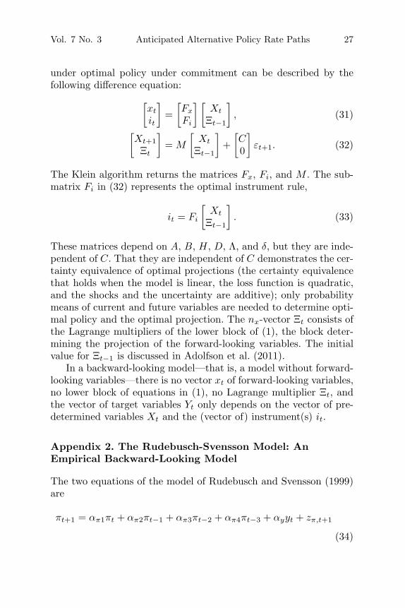
The optimal instrument rule under commitment (see appendix 1)can be written as
0 = FiXXt + FiΞΞt−1 − it, (8)
where the matrix Fi in (33) is partitioned conformably with Xt andΞt−1. Here the nx-vector of Lagrange multipliers Ξt in equilibriumfollows
Ξt = MΞXXt + MΞΞΞt−1, (9)
7A targeting rule can be expressed in terms of expected leads, current values,and lags of the target variables (the arguments of the loss function); see Svensson(1999), Svensson and Woodford (2005), and Giannoni and Woodford (2010).

Vol. 7 No. 3 Anticipated Alternative Policy Rate Paths 9
where the matrix M in (32) has been partitioned conformably withXt and Ξt−1. Thus, in order to include this optimal instrument rulein the set of policy rules (7) considered, the predetermined variablesneed to be augmented with Ξt−1 and the equations for the pre-determined variables with (9). For simplicity, the treatment belowdoes not include this augmentation. Alternatively, below the vectorof predetermined variables could consistently be augmented withthe vector of Lagrange multipliers, so everywhere we would have(X ′
t, Ξ′t−1)
′ instead of Xt, with corresponding augmentation of therelevant matrices.
The general policy rule can be added to the model equations (1)to form the new system to be solved. With the notation xt ≡ (x′
t, i′t)
′,the new system can be written[
Xt+1
Hxt+1|t
]= A
[Xt
xt
]+
[C
0(nx+ni)×nε
]εt+1, (10)
for t = . . . ,−1, 0, 1, . . ., where
H ≡[
H 0Gx Gi
], A ≡
⎡⎣A11 A12 B1
A21 A22 B2fX fx fi
⎤⎦ ,
and where H is partitioned conformably with xt and it and A ispartitioned conformably with Xt, xt, and it.
Then, under the assumption that the policy rule gives rise to thesaddlepoint property (that the number of eigenvalues with modu-lus greater than unity is equal to the number of non-predeterminedvariables), the system can be solved with the Klein (2000) algorithmor the other algorithms for the solution of linear rational expecta-tions models mentioned in the introduction. The Klein algorithmgenerates the matrices M and F such that the resulting equilibriumsatisfies
Xt+1 = MXt + Cεt+1, (11)
xt ≡[xt
it
]= FXt ≡
[Fx
Fi
]Xt (12)
for t = . . . ,−1, 0, 1, . . ., where the matrices M and F depend on Aand H, and thereby on A, B, H, G, and f .

10 International Journal of Central Banking September 2011
In a backward-looking model, the time-invariant instrument ruledepends on the vector of predetermined variables only, since thereare no forward-looking variables, and the vector xt is identical to it.
Consider now projections in period t—that is, mean forecasts,conditional on information available in period t, of future realiza-tions of the variables. For any stochastic vector process ut, letut ≡ {ut+τ,t}∞
τ=0 denote a projection in period t, where ut+τ,t
denotes the mean forecast of the realization of the vector in periodt + τ conditional on information available in period t. We refer to τas the horizon of the forecast ut+τ,t.
The projection (Xt, xt, it) in period t is then given by (11) and(12) when we set the mean of future i.i.d. shocks equal to zero,εt+τ,t = Etεt+τ = 0 for τ > 0. It then satisfies
Xt+τ,t = MτXt,t, (13)
xt+τ,t ≡[xt+τ,t
it+τ,t
]= FXt+τ,t ≡
[Fx
Fi
]Xt+τ,t =
[Fx
Fi
]MτXt,t, (14)
Xt,t = Xt|t, (15)
for τ ≥ 0, where Xt|t is the estimate of predetermined variablesin period t conditional on information available in the beginningof period t. Thus, “, t” and “t” in subindices refer to projections(forecasting) and estimates (“nowcasting” and “backcasting”) in thebeginning of period t, respectively.
3. Projections with Time-Varying Restrictions on thePolicy Rate
The projection of the policy rate it = {it+τ,t}∞τ=0 in period t is by
(14) given by
it+τ,t = FiMτXt+τ,t
for τ ≥ 0.8
8The projection of the policy rate and the other variables will satisfy the policyrule,
Gxxt+τ+1,t + Giit+τ+1,t = fXXt+τ,t + fxxt+τ,t + fiit+τ,t,
for τ ≥ 0.

Vol. 7 No. 3 Anticipated Alternative Policy Rate Paths 11
Suppose now that we consider imposing restrictions on the policyrate projection of the form
it+τ,t = ıt+τ,t, τ = 0, . . . , T, (16)
where {ıt+τ,t}Tτ=0 is a sequence of T+1 given policy rate levels. Alter-
natively, we can have restriction on the real policy rate projectionof the form
rt+τ,t = rt+τ,t, τ = 0, . . . , T, (17)
where
rt ≡ it − πt+1|t (18)
is the real policy rate and πt+1|t is expected inflation. With restric-tions of this kind, the nominal or real policy rate is exogenous forperiod t, t + 1, . . . , t + T .
These restrictions are here assumed to be anticipated by boththe central bank and the private sector, in contrast to Leeper andZha (2003) where they are anticipated and planned by the centralbank but not anticipated by the private sector. Thus, our case cor-responds to a situation where the restriction is announced to theprivate sector by the central bank and believed by the private sec-tor, whereas the Leeper and Zha case corresponds to a situationwhere the central bank either makes secret plans to implement therestriction or the restriction is announced but not believed by theprivate sector.
The restrictions make the nominal or real policy rate projectionexogenous for the periods t, t + 1, . . . , t + T . We know from Sar-gent and Wallace (1975) that exogenous interest rates may causeindeterminacy when there are forward-looking variables. In order toensure determinacy, we assume that there is an anticipated switchin period t + T + 1 to the policy rule (G, f). Then the restrictionscan be implemented by augmenting a stochastic deviation, zt, to thepolicy rule (7),
Gxxt+1|t + Giit+1|t = fXXt + fxxt + fiit + zt. (19)
The projection {zt+τ,t}Tτ=0 of the future deviations is then chosen
such that (16) or (17) is satisfied. The projection of the future
12 International Journal of Central Banking September 2011
deviation from the horizon T + 1 and beyond is zero, correspondingto the anticipated shift then to the policy rule (G, f).
More precisely, we let the (T + 1)-vector zt ≡ (zt,t, zt+1,t, . . . ,zt+T,t)′ (where zt,t = zt) denote a projection of the stochastic vari-able zt+τ for τ = 0, . . . , T . As in the treatment of central bankjudgment in Svensson (2005), the stochastic variable zt is called thedeviation. In particular, we assume that the deviation is a moving-average process that satisfies
zt = ηt,t +T∑
s=1
ηt,t−s
for a given T ≥ 0, where ηt ≡ (η′t,t, η
′t+1,t, . . . , η
′t+T,t)
′ is a zero-meani.i.d. random (T +1)-vector realized in the beginning of period t andcalled the innovation in period t. For T = 0, we have zt = ηt,t, andthe deviation is a simple i.i.d. disturbance. For T > 0, the deviationinstead follows a moving-average process. Then we have
zt+τ,t+1 = zt+τ,t + ηt+τ,t+1, τ = 1, . . . , T,
zt+T+1,t+1 = ηt+T+1,t+1.
It follows that the dynamics of the deviation and the projection zt
can be written
zt+1 = Azzt + ηt+1, (20)
where the (T + 1) × (T + 1) matrix Az is defined as
Az ≡[0T×1 IT
0 01×T
].
Hence, zt is the central bank’s mean projection of current andfuture deviations, and ηt can be interpreted as the new informationthe central bank receives in the beginning of period t about thosedeviations.9
9In Svensson (2005) the deviation zt is an nz-vector of terms entering thedifferent equations in the model, and the projection zt of future zt deviation isidentified with central bank judgment. The graphs in Svensson (2005) can be seenas impulse responses to ηt, the new information about future deviations. (Thenotation here is slightly different from Svensson 2005 in that there the projectionzt ≡ (zt+1,t, . . . , zt+T,t)′ does not include the current deviation.)

Vol. 7 No. 3 Anticipated Alternative Policy Rate Paths 13
Combining the model (1) with the augmented policy rule (19)gives the system[
Xt+1
Hxt+1|t
]= A
[Xt
xt
]+
[C
0(nx+ni)×(nε+T+1)
] [εt+1ηt+1,
](21)
for t = . . . ,−1, 0, 1, . . ., where
Xt ≡[Xt
zt
], xt ≡
[xt
it
], H ≡
[H 0Gx Gi
],
A ≡
⎡⎢⎢⎢⎢⎣
A11 0nX×1 0nX×T A12 B10T×nX
0T×1 IT 0T×nx 0T×101×nX
0 01×T 01×nx0
A21 0nx×1 0nx×T A22 B2fX 1 01×T fx fi
⎤⎥⎥⎥⎥⎦ ,
C ≡[
C 0nX×(T+1)0(T+1)×nε
IT+1
].
Under the assumption of the saddlepoint property, the systemof difference equations (21) has a unique solution and there existunique matrices M and F such that projection can be written
Xt+τ,t = Mτ Xt,t,
xt+τ,t = FXt+τ,t = FMτ Xt,t
for τ ≥ 0, where Xt,t in Xt,t ≡ (X ′t,t, z
t′)′ is given but the (T + 1)-vector zt remains to be determined. Its elements are then determinedby the restrictions (16) or (17).
In order to satisfy the restriction (16) on the nominal policy rate,we note that it can now be written
it+τ,t = FiMτ
[Xt,t
zt
]= ıt+τ,t, τ = 0, 1, . . . , T.
This provides T + 1 linear equations for the T + 1 elements of zt.In order to instead satisfy the restriction (17) on the real policy
rate, we note that inflation expectations in a DSGE model similarto Ramses generally satisfy
14 International Journal of Central Banking September 2011
πt+1|t ≡ ϕxt+1|t + Φ[Xt
xt
](22)
for some vectors ϕ and Φ. These vectors ϕ and Φ are structural, notreduced-form expressions. For instance, if πt is one of the elementsof xt, the corresponding element of ϕ is unity, all other elementsof ϕ are zero, and Φ ≡ 0. If πt+1|t is one of the elements of xt, thecorresponding element of Φ is unity, all other elements of Φ are zero,and ϕ ≡ 0. Then the restriction (17) can be written
rt+τ,t ≡ it+τ,t − πt+τ+1,t = (Fi − ϕFM − Φ)Mτ
[Xt,t
zt
]= rt+τ,t, τ = 0, 1, . . . , T.
This again provides T + 1 linear equations for the T + 1 elements ofzt.
When the restriction is on the nominal policy rate, we canthink of the equilibrium as being implemented by the central bankannouncing the nominal policy rate path and the private sectorincorporating this policy rate projection in their expectations, withthe understanding that the policy rate will be set according to thegiven policy rule (G, f) from period t + T + 1. When the restric-tion is on the real policy rate, we need to consider the fact thatin practice central banks set nominal policy rates, not real ones.The restriction on the real policy rate will result in an endogenouslydetermined nominal policy rate projection, which together with theendogenously determined inflation projection will be consistent withthe real policy rate path. We can then think of the equilibrium asbeing implemented by the central bank calculating that nominalpolicy rate projection and then announcing it to the private sector.
3.1 Backward-Looking Model
In a backward-looking model, the projection of the instrument rulewith the time-varying constraints can be written
it+τ,t = fXXt+τ,t + zt+τ,t, (23)
so it is trivial to determine the projection zt recursively so as tosatisfy the restriction (16) on the nominal policy rate projection.

Vol. 7 No. 3 Anticipated Alternative Policy Rate Paths 15
Inflation can be written
πt = ΦXt
for some vector Φ, so expected inflation can be written
πt+1|t = ΦXt+1|t = Φ(AXt + Bit). (24)
By combining (23), (24), and (18), it is trivial to determine the pro-jection zt so as to satisfy the restriction (17) on the real policy rateprojection.
4. Examples
In this section we examine restrictions on the nominal and real pol-icy rate path for the backward-looking Rudebusch-Svensson modeland the two forward-looking models, the Linde model and Ramses.Appendices 2 and 3 provide some details on the Rudebusch-Svenssonand Linde models. We also show a simulation with Ramses with themethod of modest interventions by Leeper and Zha. Appendix 4provides some details on the Leeper-Zha method.
4.1 The Rudebusch-Svensson Model
The backward-looking empirical Rudebusch-Svensson (1999) modelhas two equations (with estimates rounded to two decimal points):
πt+1 = 0.70 πt − 0.10 πt−1 + 0.28 πt−2 + 0.12 πt−3 + 0.14 yt + επ,t+1,
(25)
yt+1 = 1.16 yt − 0.25 yt−1 − 0.10(
14Σ3
j=0it−j − 14Σ3
j=0πt−j
)+ εy,t+1.
(26)
The period is a quarter, πt is quarterly GDP inflation measuredin percentage points at an annual rate, yt is the output gapmeasured in percentage points, and it is the quarterly averageof the federal funds rate, measured in percentage points at anannual rate. All variables are measured as differences from theirmeans, their steady-state levels. The predetermined variables are
16 International Journal of Central Banking September 2011
Xt ≡ (πt, πt−1, πt−2,πt−2, yt, yt−1, it−1, it−2,it−3)′. See appendix 2for details.
The target variables are inflation, the output gap, and the firstdifference of the federal funds rate. The period loss function is
Lt =12[π2
t + λyy2t + λΔi(it − it−1)2
], (27)
where πt is measured as the difference from the inflation target,which is equal to the steady-state level. The discount factor, δ, andthe relative weights on output-gap stabilization, λy, and interest ratesmoothing, λΔi, are set to satisfy δ = 1, λy = 1, and λΔi = 0.2.
For the loss function (27) with the parameters δ = 1, λy = 1,and λΔi = 0.2, and the case where εt is an i.i.d. shock with zeromean, the optimal instrument rule is as follows (the coefficients arerounded to two decimal points):
it = 1.22 πt + 0.43 πt−1 + 0.53 πt−2 + 0.18 πt−3 + 1.93 yt − 0.49 yt−1
+ 0.36 it−1 − 0.09 it−2 − 0.05 it−3.
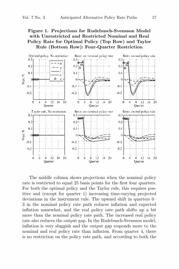
Figure 1 shows projections for the Rudebusch-Svensson model.The top row of panels shows projections under the optimal policy,whereas the bottom row of panels shows projections under a Taylorrule,
it = 1.5 πt + 0.5 yt,
where the policy rate responds to the predetermined inflation andoutput gap with the standard coefficients 1.5 and 0.5, respectively.
The projections start in quarter 0 from the steady state, whenall the predetermined variables are zero. The left column of panelsshows the projections when there is no restriction imposed on thenominal or real policy rate path. This corresponds to zero projecteddeviations zt+τ,t in the optimal instrument rule and the Taylor rule.These are denoted by circles for the first four quarters, quarters 0–3.The economy remains in the steady state, and inflation (denotedby a dashed curve), the output gap (denoted by a dashed-dottedcurve), the nominal policy rate (denoted by a solid curve), and thereal policy rate (denoted by a dotted curve) all remain at zero.
Vol. 7 No. 3 Anticipated Alternative Policy Rate Paths 17
Figure 1. Projections for Rudebusch-Svensson Modelwith Unrestricted and Restricted Nominal and Real
Policy Rate for Optimal Policy (Top Row) and TaylorRule (Bottom Row): Four-Quarter Restriction
The middle column shows projections when the nominal policyrate is restricted to equal 25 basis points for the first four quarters.For both the optimal policy and the Taylor rule, this requires pos-itive and (except for quarter 1) increasing time-varying projecteddeviations in the instrument rule. The upward shift in quarters 0–3 in the nominal policy rate path reduces inflation and expectedinflation somewhat, and the real policy rate path shifts up a bitmore than the nominal policy rate path. The increased real policyrate also reduces the output gap. In the Rudebusch-Svensson model,inflation is very sluggish and the output gap responds more to thenominal and real policy rate than inflation. From quarter 4, thereis no restriction on the policy rate path, and according to both the
18 International Journal of Central Banking September 2011
optimal policy and the Taylor rule, the nominal and real policy rateare reduced substantially so as to bring the negative inflation andoutput gap eventually back to zero. The optimal policy is more effec-tive in bringing back inflation and the output gap than the Taylorrule, which is natural since the Taylor rule is not optimal.
The right column shows projections when the real policy rate isrestricted to equal unity during quarters 0–3. Since there is so lit-tle movement in inflation and expected inflation, the projections forthese restrictions on the real and the nominal policy rate are verysimilar.
Since there are no forward-looking variables in the Rudebusch-Svensson model, there would be no difference between these pro-jections with anticipated restrictions on the policy rate path andsimulations with unanticipated shocks as in Leeper and Zha (2003).
4.2 The Linde Model
The empirical New Keynesian model of the U.S. economy due toLinde (2005) also has two equations. We use the following parameterestimates:
πt = 0.457 πt+1|t + (1 − 0.457)πt−1 + 0.048yt + επt,
yt = 0.425 yt+1|t + (1 − 0.425)yt−1 − 0.156(it − πt+1|t) + εyt.
The period is a quarter, and πt is quarterly GDP inflation measuredin percentage points at an annual rate, yt is the output gap meas-ured in percentage points, and it is the quarterly average of the fed-eral funds rate, measured in percentage points at an annual rate.All variables are measured as differences from their means, theirsteady-state levels. The shock εt ≡ (επt, εyt)′ is i.i.d. with meanzero.
For the loss function (27), the predetermined variables are Xt ≡(επt, εyt, πt−1, yt−1, it−1)′ (the lagged policy rate enters because itenters into the loss function, and the two shocks are included amongthe predetermined variables in order to write the model on theform (1) with no shocks in the equations for the forward-looking

Vol. 7 No. 3 Anticipated Alternative Policy Rate Paths 19
variables). The forward-looking variables are xt ≡ (πt, yt)′. Seeappendix 3 for details.10
For the loss function (27) with the parameters δ = 1, λy = 1,and λΔi = 0.2, the optimal policy function (8) is as follows (thecoefficients are rounded to two decimal points):
it = 1.06 επt + 1.38 εyt + 0.58 πt−1 + 0.78 yt−1 + 0.40 it−1
+ 0.02 Ξπ,t−1,t−1 + 0.20 Ξy,t−1,t−1,
where Ξπ,t−1,t−1 and Ξy,t−1,t−1 are the Lagrange multipliers for thetwo equations for the forward-looking variables in the decision prob-lem in period t − 1 (see appendix 1). The difference equation (9) forthe Lagrange multipliers is
[Ξπt
Ξyt
]=
[10.20 0.74 5.54 0.43 −0.210.74 1.48 0.40 0.85 −0.28
]⎡⎢⎢⎢⎢⎣
επt
εyt
πt−1yt−1it−1
⎤⎥⎥⎥⎥⎦
+[0.72 0.160.03 0.38
] [Ξπ,t−1Ξy,t−1
].
We also examine the projections for a Taylor rule for which thepolicy rate responds to current inflation and the output gap,
it = 1.5 πt + 0.5 yt.
Figure 2 shows projections for the optimal policy (top row) andTaylor rule (bottom row) when there is a restriction to equal 25 basispoints for quarters 0–3 for the nominal policy rate (middle column)and the real policy rate (right column). In the middle column, wesee that a restriction to a 25-basis-points-higher nominal policy ratereduces inflation and inflation expectations so the projection of the
10It is arguably unrealistic to consider inflation and output in the current quar-ter as forward-looking variables. Alternatively, current inflation and the outputgap could be treated as predetermined, and one-quarter-ahead plans for inflation,the output gap, and the policy rate could be determined by the model above.Such a variant of the New Keynesian model is used in Svensson and Woodford(2005).
20 International Journal of Central Banking September 2011
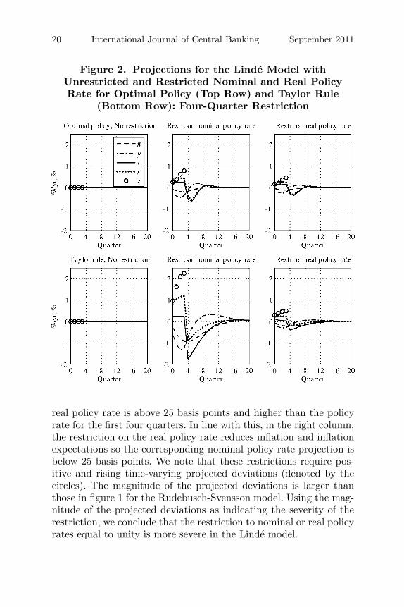
Figure 2. Projections for the Linde Model withUnrestricted and Restricted Nominal and Real PolicyRate for Optimal Policy (Top Row) and Taylor Rule
(Bottom Row): Four-Quarter Restriction
real policy rate is above 25 basis points and higher than the policyrate for the first four quarters. In line with this, in the right column,the restriction on the real policy rate reduces inflation and inflationexpectations so the corresponding nominal policy rate projection isbelow 25 basis points. We note that these restrictions require pos-itive and rising time-varying projected deviations (denoted by thecircles). The magnitude of the projected deviations is larger thanthose in figure 1 for the Rudebusch-Svensson model. Using the mag-nitude of the projected deviations as indicating the severity of therestriction, we conclude that the restriction to nominal or real policyrates equal to unity is more severe in the Linde model.

Vol. 7 No. 3 Anticipated Alternative Policy Rate Paths 21
Figure 3. Projections for Ramses with AnticipatedUnrestricted and Restricted Nominal and Real Policy
Rate (Top Row) and Unanticipated Restrictions on theNominal Policy Rate (Bottom Row): Four-Quarter
Restriction
Because inflation is more sensitive to movements in the real pol-icy rate in the Linde model than in the Rudebusch-Svensson model,there is a greater difference between restrictions on the nominal andthe real policy rate. Also, from quarter 4, when there is no restric-tion on the policy rate, a fall in the real and nominal policy rate,according to both the optimal policy and the Taylor rule, more eas-ily stabilizes inflation and the output gap back to the steady statethan in the Rudebusch-Svensson model.
4.3 Ramses
Adolfson et al. (2011) provide more details on Ramses, including theelements of the vectors Xt, xt, it, and εt. Figure 3 shows projections

22 International Journal of Central Banking September 2011
with Ramses for the estimated instrument rule. The top row showsthe result of restrictions on the nominal and real policy rate to equal25 basis points for four quarters, quarters 0–3. We see that there isa substantial difference between restrictions on the nominal and thereal policy rate, since inflation is quite sensitive to the real policyrate in Ramses. In the top-middle panel, we see that a restrictionon the nominal policy rate projection to equal 25 basis points forquarters 0–3 corresponds to a very high and falling real policy rateprojection. In the top-right panel we see that the restriction on thereal policy rate to equal 25 basis points for quarters 0–3 correspondsto a nominal policy rate projection quite a bit below the real policyrate.
The bottom panel of figure 3 shows the result of a projectionwith the Leeper-Zha method of modest interventions to implementa restriction on the nominal policy rate to equal 25 basis pointsfor quarters 0–3. There, positive unanticipated shocks (denoted bycircles) are added to the estimated instrument rule to achieve therestriction on the nominal policy rate. Comparing the bottom panelwith the top-right panel, we see that the impact on inflation, the out-put gap, and the real interest rate is smaller for the unanticipatedshocks in the Leeper-Zha method than for the anticipated projecteddeviations in our method.
4.4 Unusual Equilibria
If restrictions are imposed on the nominal policy rate for many peri-ods, “unusual” equilibria can occur. We can illustrate this for Ram-ses in figure 4, where in the top-middle panel the nominal policyrate is restricted to equal 25 basis points for nine quarters, quarters0–8. This is a very contractionary policy, which shows in inflationand inflation expectations falling very much and the real policy ratebecoming very high. (Note that the scale varies from panel to panelin figure 4.) If we look at the top-right panel, where the real pol-icy rate is restricted to equal 25 basis points for nine quarters, wesee that inflation and inflation expectations fall so much that thenominal policy rate becomes negative in quarter 0 (relative to whenthere is no restriction) and then rises to become positive only inquarters 7 and 8. We realize that if inflation and inflation expecta-tions respond so much that nominal and real policy rates move in
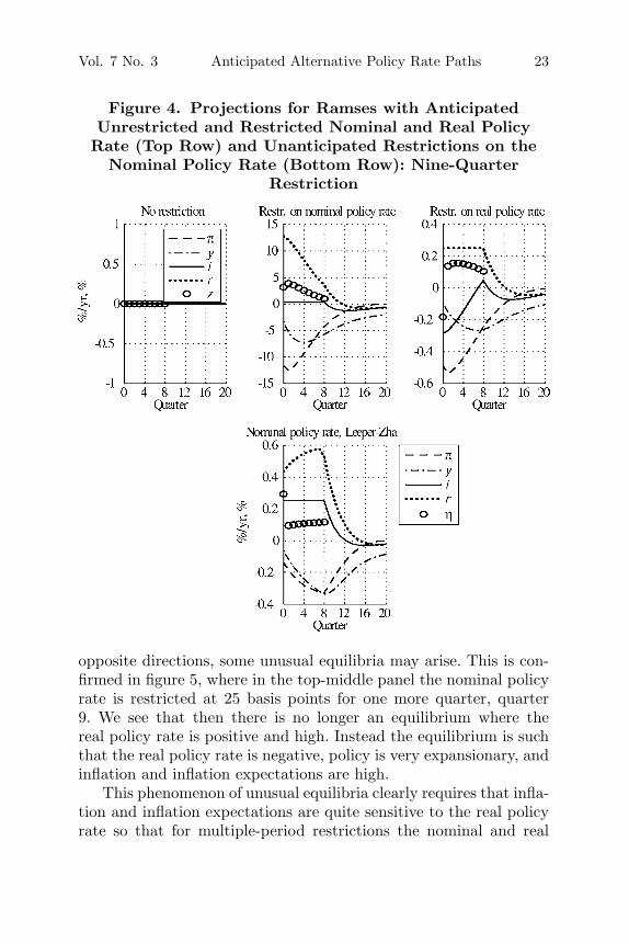
Vol. 7 No. 3 Anticipated Alternative Policy Rate Paths 23
Figure 4. Projections for Ramses with AnticipatedUnrestricted and Restricted Nominal and Real Policy
Rate (Top Row) and Unanticipated Restrictions on theNominal Policy Rate (Bottom Row): Nine-Quarter
Restriction
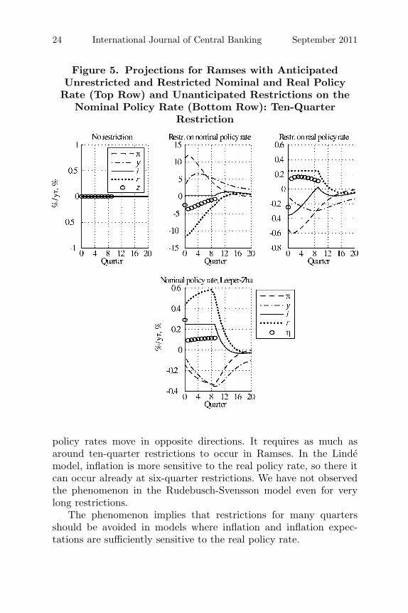
opposite directions, some unusual equilibria may arise. This is con-firmed in figure 5, where in the top-middle panel the nominal policyrate is restricted at 25 basis points for one more quarter, quarter9. We see that then there is no longer an equilibrium where thereal policy rate is positive and high. Instead the equilibrium is suchthat the real policy rate is negative, policy is very expansionary, andinflation and inflation expectations are high.
This phenomenon of unusual equilibria clearly requires that infla-tion and inflation expectations are quite sensitive to the real policyrate so that for multiple-period restrictions the nominal and real
24 International Journal of Central Banking September 2011
Figure 5. Projections for Ramses with AnticipatedUnrestricted and Restricted Nominal and Real Policy
Rate (Top Row) and Unanticipated Restrictions on theNominal Policy Rate (Bottom Row): Ten-Quarter
Restriction
policy rates move in opposite directions. It requires as much asaround ten-quarter restrictions to occur in Ramses. In the Lindemodel, inflation is more sensitive to the real policy rate, so there itcan occur already at six-quarter restrictions. We have not observedthe phenomenon in the Rudebusch-Svensson model even for verylong restrictions.
The phenomenon implies that restrictions for many quartersshould be avoided in models where inflation and inflation expec-tations are sufficiently sensitive to the real policy rate.

Vol. 7 No. 3 Anticipated Alternative Policy Rate Paths 25
5. Conclusions
We have presented a new convenient way to construct projectionsconditional on alternative anticipated policy rate paths in linearizeddynamic stochastic general equilibrium (DSGE) models, such asRamses, the Riksbank’s main DSGE model. The main idea is toinclude the anticipated future time-varying deviations from a policyrule in the vector of predetermined variables, the “state” of the econ-omy. This allows the formulation of the linear(ized) model on a stan-dard state-space form, the application of standard algorithms for thesolution of linear rational expectations models, and a recursive repre-sentation of the equilibrium projections. Projections for anticipatedpolicy rate paths are especially relevant for central banks—such asthe Reserve Bank of New Zealand, Norges Bank, the Riksbank, andthe Czech National Bank—that publish a policy rate path, but theyare also relevant for the discussion of the kind of “forward guidance”recently given by the Federal Reserve and Bank of Canada.
From the examples in this paper, we have seen that in a modelwithout forward-looking variables such as the empirical model of theU.S. economy by Rudebusch and Svensson (1999), there is no differ-ence between policy simulations with anticipated and unanticipatedrestrictions on the policy rate path. In a model with forward-lookingvariables, such as Ramses or the empirical New Keynesian model ofthe U.S. economy by Linde (2005), there is such a difference, andthe impact of anticipated deviations from a policy rule will gener-ally be larger than that of unanticipated deviations. In a model withforward-looking variables, exogenous restrictions on the policy ratepath are consistent with a unique equilibrium, if there is an antici-pated switch to a well-behaved policy rule in the future. For givenrestrictions on the policy rate path, the equilibrium depends on thatpolicy rule.
Furthermore, our analysis shows that if inflation is sufficientlysensitive to the real policy rate, “unusual” equilibria may resultfrom restrictions on the nominal policy rate for sufficiently manyperiods. Such cases have the property that nominal and real pol-icy rates move in opposite directions and nominal policy rates andinflation (expectations) move in the same direction. This phenome-non implies that restrictions on nominal policy rates for too manyperiods should be avoided.
26 International Journal of Central Banking September 2011
Appendix 1. Optimal Policy
Let Yt be an nY -vector of target variables, measured as the differ-ence from an nY -vector Y ∗ of target levels. This is not restrictive, aslong as we keep the target levels time invariant. If we would like toexamine the consequences of different target levels, we can insteadinterpret Yt as the absolute level of the target levels and replace Yt
with Yt −Y ∗ everywhere below. We assume that the target variablescan be written as a linear function of the predetermined variables,the forward-looking variables, and the instruments,
Yt = D
⎡⎣Xt
xt
it
⎤⎦ ≡ [DX Dx Di]
⎡⎣Xt
xt
it
⎤⎦ , (28)
where D is an nY × (nX + nx + ni) matrix and partitioned con-formably with Xt, xt, and it.
Let the intertemporal loss function in period t be
Et
∞∑τ=0
δτLt+τ , (29)
where 0 < δ < 1 is a discount factor, Lt is the period loss given by
Lt ≡ Y ′t ΛYt, (30)
and Λ is a symmetric positive semi-definite matrix containing theweights on the individual target variables.11
Optimization under commitment in a timeless perspective(Woodford 2003), combined with the model equations (1), results ina system of difference equations (see Soderlind 1999 and Svensson2009). The system of difference equations can be solved with sev-eral alternative algorithms—for instance, those developed by Klein(2000) and Sims (2000) or the AIM algorithm of Anderson andMoore (1983, 1985) (see Svensson 2005, 2009 for details of the deriva-tion and the application of the Klein algorithm). The equilibrium
11For plotting and other purposes, and to avoid unnecessary separate programcode, it is convenient to expand the vector Yt to include a number of variablesof interest that are not necessary target variables or potential target variables.These will then have zero weight in the loss function.
Vol. 7 No. 3 Anticipated Alternative Policy Rate Paths 27
under optimal policy under commitment can be described by thefollowing difference equation:[
xt
it
]=
[Fx
Fi
] [Xt
Ξt−1
], (31)[
Xt+1Ξt
]= M
[Xt
Ξt−1
]+
[C0
]εt+1. (32)
The Klein algorithm returns the matrices Fx, Fi, and M . The sub-matrix Fi in (32) represents the optimal instrument rule,
it = Fi
[Xt
Ξt−1
]. (33)
These matrices depend on A, B, H, D, Λ, and δ, but they are inde-pendent of C. That they are independent of C demonstrates the cer-tainty equivalence of optimal projections (the certainty equivalencethat holds when the model is linear, the loss function is quadratic,and the shocks and the uncertainty are additive); only probabilitymeans of current and future variables are needed to determine opti-mal policy and the optimal projection. The nx-vector Ξt consists ofthe Lagrange multipliers of the lower block of (1), the block deter-mining the projection of the forward-looking variables. The initialvalue for Ξt−1 is discussed in Adolfson et al. (2011).
In a backward-looking model—that is, a model without forward-looking variables—there is no vector xt of forward-looking variables,no lower block of equations in (1), no Lagrange multiplier Ξt, andthe vector of target variables Yt only depends on the vector of pre-determined variables Xt and the (vector of) instrument(s) it.
Appendix 2. The Rudebusch-Svensson Model: AnEmpirical Backward-Looking Model
The two equations of the model of Rudebusch and Svensson (1999)are
πt+1 = απ1πt + απ2πt−1 + απ3πt−2 + απ4πt−3 + αyyt + zπ,t+1
(34)

28 International Journal of Central Banking September 2011
yt+1 = βy1yt + βy2yt−1 − βr
(14Σ3
j=0it−j − 14Σ3
j=0πt−j
)+ zy,t+1,
(35)
where πt is quarterly inflation in the GDP chain-weighted price index(Pt) in percentage points at an annual rate, i.e., 400(lnPt − lnPt−1);it is the quarterly average federal funds rate in percentage pointsat an annual rate; and yt is the relative gap between actual realGDP (Qt) and potential GDP (Q∗
t ) in percentage points, i.e.,100(Qt − Q∗
t )/Q∗t . These five variables were demeaned prior to esti-
mation, so no constants appear in the equations.The estimated parameters, using the sample period 1961:Q1 to
1996:Q2, are shown in table 1.
Table 1. Estimated Parameters, Rudebusch-SvenssonModel
απ1 απ2 απ3 απ4 αy βy1 βy2 βr
0.70 −0.10 0.28 0.12 0.14 1.16 −0.25 0.10(0.08) (0.10) (0.10) (0.08) (0.03) (0.08) (0.08) (0.03)
The hypothesis that the sum of the lag coefficients of inflationequals one has a p-value of .16, so this restriction was imposed inthe estimation.
The state-space form can be written⎡⎢⎢⎢⎢⎢⎢⎢⎢⎢⎢⎢⎢⎢⎣
πt+1
πt
πt−1
πt−2
yt+1
yt
itit−1
it−2
⎤⎥⎥⎥⎥⎥⎥⎥⎥⎥⎥⎥⎥⎥⎦=
⎡⎢⎢⎢⎢⎢⎢⎢⎢⎢⎢⎢⎢⎢⎣
∑4j=1 απjej + αye5
e1
e2
e3
βre1:4 + βy1e5 + βy2e6 − βre7:9
e5
e0
e7
e8
⎤⎥⎥⎥⎥⎥⎥⎥⎥⎥⎥⎥⎥⎥⎦
⎡⎢⎢⎢⎢⎢⎢⎢⎢⎢⎢⎢⎢⎢⎣
πt
πt−1
πt−2
πt−3
yt
yt−1
it−1
it−2
it−3
⎤⎥⎥⎥⎥⎥⎥⎥⎥⎥⎥⎥⎥⎥⎦
+
⎡⎢⎢⎢⎢⎢⎢⎢⎢⎢⎢⎢⎢⎢⎣
0000
−βr
40100
⎤⎥⎥⎥⎥⎥⎥⎥⎥⎥⎥⎥⎥⎥⎦
it+
⎡⎢⎢⎢⎢⎢⎢⎢⎢⎢⎢⎢⎢⎢⎣
zπ,t+1
000
zy,t+1
0000
⎤⎥⎥⎥⎥⎥⎥⎥⎥⎥⎥⎥⎥⎥⎦
,
where ej (j = 0, 1, . . . , 9) denotes a 1×9 row vector, for j = 0 withall elements equal to zero, for j = 1, . . . , 9 with element j equal tounity and all other elements equal to zero; and where ej:k (j < k)
Vol. 7 No. 3 Anticipated Alternative Policy Rate Paths 29
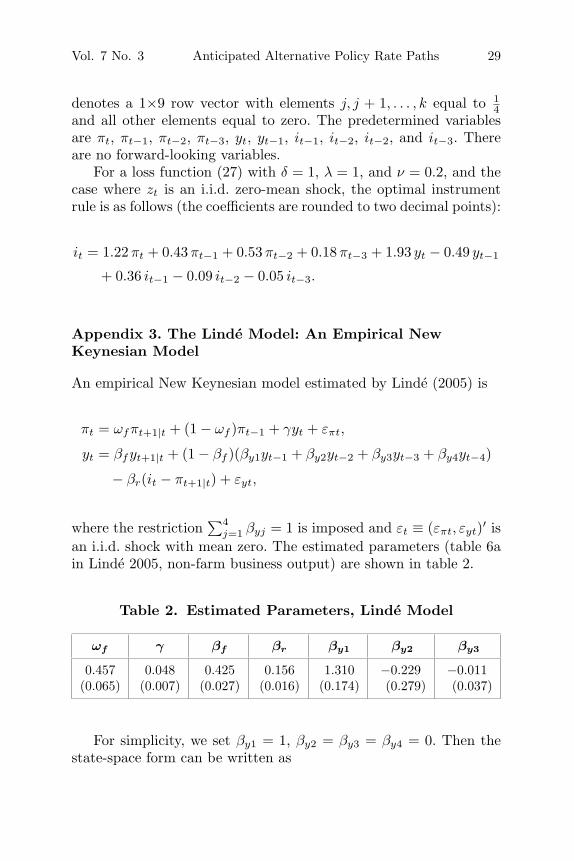
denotes a 1×9 row vector with elements j, j + 1, . . . , k equal to 14
and all other elements equal to zero. The predetermined variablesare πt, πt−1, πt−2, πt−3, yt, yt−1, it−1, it−2, it−2, and it−3. Thereare no forward-looking variables.
For a loss function (27) with δ = 1, λ = 1, and ν = 0.2, and thecase where zt is an i.i.d. zero-mean shock, the optimal instrumentrule is as follows (the coefficients are rounded to two decimal points):
it = 1.22 πt + 0.43 πt−1 + 0.53 πt−2 + 0.18 πt−3 + 1.93 yt − 0.49 yt−1
+ 0.36 it−1 − 0.09 it−2 − 0.05 it−3.
Appendix 3. The Linde Model: An Empirical NewKeynesian Model
An empirical New Keynesian model estimated by Linde (2005) is
πt = ωfπt+1|t + (1 − ωf )πt−1 + γyt + επt,
yt = βfyt+1|t + (1 − βf )(βy1yt−1 + βy2yt−2 + βy3yt−3 + βy4yt−4)
− βr(it − πt+1|t) + εyt,
where the restriction∑4
j=1 βyj = 1 is imposed and εt ≡ (επt, εyt)′ isan i.i.d. shock with mean zero. The estimated parameters (table 6ain Linde 2005, non-farm business output) are shown in table 2.
Table 2. Estimated Parameters, Linde Model
ωf γ βf βr βy1 βy2 βy3
0.457 0.048 0.425 0.156 1.310 −0.229 −0.011(0.065) (0.007) (0.027) (0.016) (0.174) (0.279) (0.037)
For simplicity, we set βy1 = 1, βy2 = βy3 = βy4 = 0. Then thestate-space form can be written as

30 International Journal of Central Banking September 2011
⎡⎢⎢⎢⎢⎢⎢⎢⎢⎢⎢⎣
επ,t+1
εy,t+1
πt
yt
it
ωfπt+1|t
βrπt+1|t + βfyt+1|t
⎤⎥⎥⎥⎥⎥⎥⎥⎥⎥⎥⎦
=
⎡⎢⎢⎢⎢⎢⎢⎢⎢⎢⎢⎣
0 0 0 0 0 0 00 0 0 0 0 0 00 0 0 0 0 1 00 0 0 0 0 0 10 0 0 0 0 0 0
−1 0 −(1 − ωf ) 0 0 1 −γ
0 −1 0 −(1 − βf ) 0 0 1
⎤⎥⎥⎥⎥⎥⎥⎥⎥⎥⎥⎦
⎡⎢⎢⎢⎢⎢⎢⎢⎢⎢⎢⎣
επt
εyt
πt−1
yt−1
it−1
πt
yt
⎤⎥⎥⎥⎥⎥⎥⎥⎥⎥⎥⎦
+
⎡⎢⎢⎢⎢⎢⎢⎢⎢⎢⎢⎣
000010βr
⎤⎥⎥⎥⎥⎥⎥⎥⎥⎥⎥⎦
it +
⎡⎢⎢⎢⎢⎢⎢⎢⎢⎢⎢⎣
επ,t+1
εy,t+1
00000
⎤⎥⎥⎥⎥⎥⎥⎥⎥⎥⎥⎦
.
The predetermined variables are επt, εyt, πt−1, yt−1, and it−1, andthe forward-looking variables are πt and yt.
For a loss function (27) with δ = 1, λy = 1, and λΔi = 0.2, andthe case where εt is an i.i.d. zero-mean shock, the optimal instru-ment rule is as follows (the coefficients are rounded to two decimalpoints):
it = 1.06 επt + 1.38 εyt + 0.58 πt−1 + 0.78 yt−1 + 0.40 it−1
+ 0.02 Ξπ,t−1,t−1 + 0.20 Ξy,t−1,t−1,
where Ξπ,t−1,t−1 and Ξy,t−1,t−1 are the Lagrange multipliers for thetwo equations for the forward-looking variables in the decision prob-lem in period t − 1. The difference equation (9) for the Lagrangemultipliers is
[Ξπt
Ξyt
]=
[10.20 0.74 5.54 0.43 −0.210.74 1.48 0.40 0.85 −0.28
]⎡⎢⎢⎢⎢⎣
επt
εyt
πt−1yt−1it−1
⎤⎥⎥⎥⎥⎦
+[0.72 0.160.03 0.38
] [Ξπ,t−1Ξy,t−1
].
Vol. 7 No. 3 Anticipated Alternative Policy Rate Paths 31
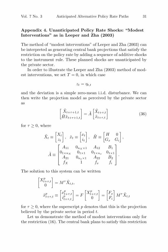
Appendix 4. Unanticipated Policy Rate Shocks: “ModestInterventions” as in Leeper and Zha (2003)
The method of “modest interventions” of Leeper and Zha (2003) canbe interpreted as generating central bank projections that satisfy therestriction on the policy rate by adding a sequence of additive shocksto the instrument rule. These planned shocks are unanticipated bythe private sector.
In order to illustrate the Leeper and Zha (2003) method of mod-est interventions, we set T = 0, in which case
zt = ηt,t
and the deviation is a simple zero-mean i.i.d. disturbance. We canthen write the projection model as perceived by the private sectoras [
Xt+τ+1,t
Hxt+τ+1,t
]= A
[Xt+τ,t
xt+τ,t
](36)
for τ ≥ 0, where
Xt ≡[Xt
zt
], xt ≡
[xt
it
], H ≡
[H 0Gx Gi
],
A ≡
⎡⎢⎢⎣
A11 0nX×1 A12 B101×nX
01×1 01×nx 01×1A21 0nx×1 A22 B2fX 1 fx fi
⎤⎥⎥⎦ .
The solution to this system can be written[Xp
t+τ,t
0
]= Mτ Xt,t,
xpt+τ,t ≡
[xp
t+τ,t
ipt+τ,t
]= F
[Xp
t+τ,t
0
]=
[Fx
Fi
]Mτ Xt,t
for τ ≥ 0, where the superscript p denotes that this is the projectionbelieved by the private sector in period t.
Let us demonstrate the method of modest interventions only forthe restriction (16). The central bank plans to satisfy this restriction
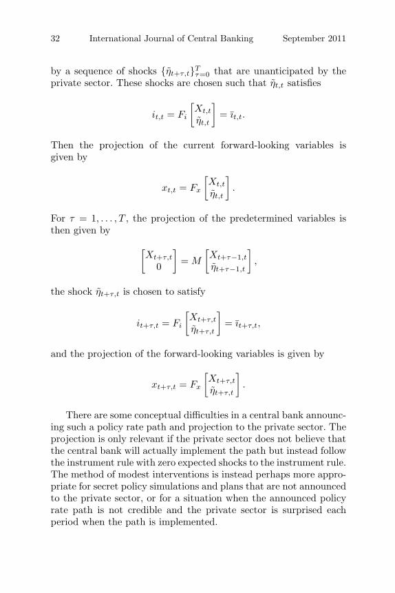
32 International Journal of Central Banking September 2011
by a sequence of shocks {ηt+τ,t}Tτ=0 that are unanticipated by the
private sector. These shocks are chosen such that ηt,t satisfies
it,t = Fi
[Xt,t
ηt,t
]= ıt,t.
Then the projection of the current forward-looking variables isgiven by
xt,t = Fx
[Xt,t
ηt,t
].
For τ = 1, . . . , T , the projection of the predetermined variables isthen given by
[Xt+τ,t
0
]= M
[Xt+τ−1,t
ηt+τ−1,t
],
the shock ηt+τ,t is chosen to satisfy
it+τ,t = Fi
[Xt+τ,t
ηt+τ,t
]= ıt+τ,t,
and the projection of the forward-looking variables is given by
xt+τ,t = Fx
[Xt+τ,t
ηt+τ,t
].
There are some conceptual difficulties in a central bank announc-ing such a policy rate path and projection to the private sector. Theprojection is only relevant if the private sector does not believe thatthe central bank will actually implement the path but instead followthe instrument rule with zero expected shocks to the instrument rule.The method of modest interventions is instead perhaps more appro-priate for secret policy simulations and plans that are not announcedto the private sector, or for a situation when the announced policyrate path is not credible and the private sector is surprised eachperiod when the path is implemented.

Vol. 7 No. 3 Anticipated Alternative Policy Rate Paths 33
References
Adolfson, M., S. Laseen, J. Linde, and L. E. O. Svensson. 2011.“Optimal Monetary Policy in an Operational Medium-SizedDSGE Model.” Forthcoming in Journal of Money, Credit, andBanking.
Adolfson, M., S. Laseen, J. Linde, and M. Villani. 2007a. “BayesianEstimation of an Open Economy DSGE Model with IncompletePass-Through.” Journal of International Economics 72 (2): 481–511.
———. 2007b. “RAMSES — A New General Equilibrium Modelfor Monetary Policy Analysis.” Economic Review (Sveriges Riks-bank) 2007 (2): 5–39.
———. 2008. “Evaluating an Estimated New Keynesian Small OpenEconomy Model.” Journal of Economic Dynamics and Control32 (8): 2690–2721.
Anderson, G. S., and G. Moore. 1983. “An Efficient Procedure forSolving Linear Perfect Foresight Models.” Working Paper. Avail-able at http://www.frb.gov.
———. 1985. “A Linear Algebraic Procedure for Solving LinearPerfect Foresight Models.” Economics Letters 17 (3): 247–52.
Boucekkine, R. 1995. “An Alternative Method for Solving NonlinearForward-Looking Models.” Journal of Economic Dynamics andControl 19 (4): 711–34.
Dynare. 2009. Dynare Manual, version 4.1.0. Available athttp://www.dynare.org.
Fair, R. C., and J. B. Taylor. 1983. “Solution and Maximum Like-lihood Estimation of Dynamic Nonlinear Rational ExpectationsModels.” Econometrica 51 (4): 1169–85.
Gagnon, J. E., and D. W. Henderson. 1990. “Nominal Interest RatePegging under Alternative Expectations Hypotheses.” In Finan-cial Sectors in Open Economies: Empirical Analysis and PolicyIssues, ed. P. Hopper, K. H. Johnson, D. L. Kohn, D. E. Lindsey,R. D. Porter, and R. Tryon, 437–73. Washington, DC: Board ofGovernors of the Federal Reserve System.
Galı, J. 2010. “Are Central Banks’ Projections Meaningful?” Work-ing Paper. Available at http://www.crei.cat/people/gali.
Giannoni, M. P., and M. Woodford. 2010. “Optimal Targeting Cri-teria for Stabilization Policy.” Working Paper.
34 International Journal of Central Banking September 2011
Juillard, M. 1996. “DYNARE: A Program for the Resolution andSimulation of Dynamic Models with Forward Variables Throughthe Use of a Relaxation Algorithm.” CEPREMAP WorkingPaper No. 9602.
Klein, P. 2000. “Using the Generalized Schur Form to Solve a Mul-tivariate Linear Rational Expectations Model.” Journal of Eco-nomic Dynamics and Control 24 (10): 1405–23.
Laffargue, J.-P. 1990. “Resolution d’un modele macroeconomiqueavec anticipations rationnelles.” Annales d’Economie et de Sta-tistique 17: 97–119.
Leeper, E. M., and T. Zha. 2003. “Modest Policy Interventions.”Journal of Monetary Economics 50 (8): 1673–1700.
Linde, J. 2005. “Estimating New-Keynesian Phillips Curves: A FullInformation Maximum Likelihood Approach.” Journal of Mone-tary Economics 52 (6): 1135–49.
Rudebusch, G. D., and L. E. O. Svensson. 1999. “Policy Rules forInflation Targeting.” In Monetary Policy Rules, ed. J. B. Taylor.Chicago: University of Chicago Press.
Sargent, T. J., and N. Wallace. 1975. “Rational Expectations, theOptimal Monetary Instrument and the Optimal Money SupplyRule.” Journal of Political Economy 83 (2): 241–54.
Sims, C. A. 2000. “Solving Linear Rational Expectations Models.”Working Paper.
Soderlind, P. 1999. “Solution and Estimation of RE Macromod-els with Optimal Policy.” European Economic Review 43 (4–6): 813–23. Related software available at http://home.tiscalinet.ch/paulsoderlind.
Svensson, L. E. O. 1999. “Inflation Targeting as a Monetary PolicyRule.” Journal of Monetary Economics 43 (3): 607–54.
———. 2005. “Monetary Policy with Judgment: Forecast Target-ing.” International Journal of Central Banking 1 (1): 1–54.
———. 2009. “Optimization under Commitment and Discretion,the Recursive Saddlepoint Method, and Targeting Rules andInstrument Rules: Lecture Notes.” Available at http://www.larseosvensson.net.
———. 2010. “Some Problems with Swedish Monetary Policy andPossible Solutions.” Speech given in Stockholm, Sweden, Novem-ber 24. Available at http://www.larseosvensson.net.
Vol. 7 No. 3 Anticipated Alternative Policy Rate Paths 35
Svensson, L. E. O., and R. J. Tetlow. 2005. “Optimal Policy Projec-tions.” International Journal of Central Banking 1 (3): 177–207.
Svensson, L. E. O., and M. Woodford. 2005. “Implementing OptimalPolicy through Inflation-Forecast Targeting.” In The Inflation-Targeting Debate, ed. B. S. Bernanke and M. Woodford, 19–83.Chicago: University of Chicago Press.
Woodford, M. 2003. Interest Rates and Prices. Princeton, NJ:Princeton University Press.


![2000 AP Macro Exam [with some 1995 & 1990 questions]...c. They can be anticipated and offset with appropriate fiscal policy. d. They can be anticipated and offset with appropriate](https://static.fdocuments.in/doc/165x107/606bd5875b97b1710e1f9a6c/2000-ap-macro-exam-with-some-1995-1990-questions-c-they-can-be-anticipated.jpg)