Antennas and Propagation Components -...

Antennas and Propagation Components

December 2003

Notice

The information contained in this document is subject to change without notice.

Agilent Technologies makes no warranty of any kind with regard to this material,including, but not limited to, the implied warranties of merchantability and fitnessfor a particular purpose. Agilent Technologies shall not be liable for errors containedherein or for incidental or consequential damages in connection with the furnishing,performance, or use of this material.

Warranty

A copy of the specific warranty terms that apply to this software product is availableupon request from your Agilent Technologies representative.

Restricted Rights Legend

Use, duplication or disclosure by the U. S. Government is subject to restrictions as setforth in subparagraph (c) (1) (ii) of the Rights in Technical Data and ComputerSoftware clause at DFARS 252.227-7013 for DoD agencies, and subparagraphs (c) (1)and (c) (2) of the Commercial Computer Software Restricted Rights clause at FAR52.227-19 for other agencies.

Agilent Technologies395 Page Mill RoadPalo Alto, CA 94304 U.S.A.

Copyright © 1998-2003, Agilent Technologies. All Rights Reserved.

Acknowledgments

Mentor Graphics is a trademark of Mentor Graphics Corporation in the U.S. andother countries.

Microsoft®, Windows®, MS Windows®, Windows NT®, and MS-DOS® are U.S.registered trademarks of Microsoft Corporation.

Pentium® is a U.S. registered trademark of Intel Corporation.

PostScript® and Acrobat® are trademarks of Adobe Systems Incorporated.

UNIX® is a registered trademark of the Open Group.

Java™ is a U.S. trademark of Sun Microsystems, Inc.

ii

Contents1 Antennas and Propagation Components

Introduction............................................................................................................... 1-1Multipath and Fading ................................................................................................ 1-4Pathloss.................................................................................................................... 1-8References ............................................................................................................... 1-9AntArray.................................................................................................................... 1-10AntBase .................................................................................................................... 1-13AntMobile.................................................................................................................. 1-15Fader ........................................................................................................................ 1-17PropFlatEarth ........................................................................................................... 1-20PropGSM.................................................................................................................. 1-23PropNADCcdma....................................................................................................... 1-30PropNADCtdma........................................................................................................ 1-34PropWCDMA............................................................................................................ 1-38UserDefChannel ....................................................................................................... 1-42UserDefVectorChannel ............................................................................................. 1-45WCDMAVectorChannel ............................................................................................ 1-47

Index

iii

Chapter 1: Antennas and PropagationComponents

IntroductionAntenna and propagation models simulate the effects of radio channel on thetransmitted signal. These effects include signal fading and pathloss. Both antennaand propagation channel models are TSDF components with input and output timedsignals.

Antenna models are identified by their coordinate and gain. For mobile antennas, thevelocity vector is also included in the parameters. The input of antennas are multi toprovide flexibility of adding the contribution from various noise or fading channels.The propagation channel models are typically identified by the type of fading, thespecification of power delay profile, and whether pathloss is to be activated.

The input as well as output impedance of antennas and channel models are left asinfinite and zero, respectively. For the inclusion of antenna impedance, cosimulationwith Circuit Envelope is recommended (for details, refer to “Introduction: CircuitCosimulation Components). In this application, S-parameter block representingmeasurement (file), functions or impedance components can be placed on the circuitschematic page and co-simulated with signal processing designs. To access anexample that demonstrates this: from the Main window, choose File > ExampleProject > Antennas-Prop > RadioChannel_prj; from the Schematic window, chooseFile > Open Design, ANTLOAD.dsn.

The separate specification of antennas and (propagation) channel components is toprovide a more intuitive and flexible use model. During the simulation, the effects ofboth antenna and channel models are merged and the combined antenna andpropagation channel components are replaced with equivalent models in thepre-processing phase of the simulation.

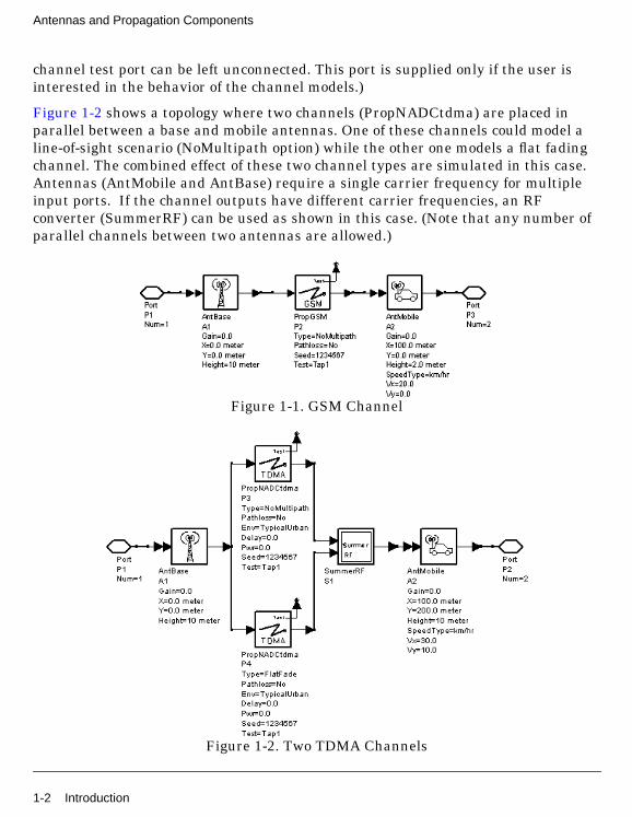
Because of interdependency of antennas and channel models, certain restrictions intopology must be considered by the user: there should be at least one propagationchannel between a pair of transmit and receive antennas. Examples of commonantenna and propagation channel connections are shown in Figure 1-1 throughFigure 1-4.

Figure 1-1 depicts the most common use model where a channel (PropGSM) is placedbetween a base station (AntBase) and mobile (AntMobile) antennas. (Note that the

Introduction 1-1


channel test port can be left unconnected. This port is supplied only if the user isinterested in the behavior of the channel models.)

Figure 1-2 shows a topology where two channels (PropNADCtdma) are placed inparallel between a base and mobile antennas. One of these channels could model aline-of-sight scenario (NoMultipath option) while the other one models a flat fadingchannel. The combined effect of these two channel types are simulated in this case.Antennas (AntMobile and AntBase) require a single carrier frequency for multipleinput ports. If the channel outputs have different carrier frequencies, an RFconverter (SummerRF) can be used as shown in this case. (Note that any number ofparallel channels between two antennas are allowed.)

Figure 1-1. GSM Channel

Figure 1-2. Two TDMA Channels

1-2 Introduction

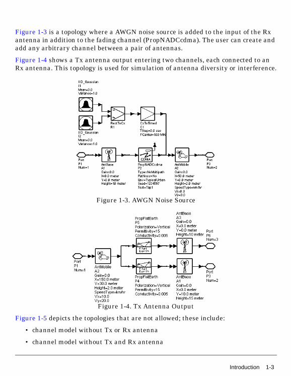
Figure 1-3 is a topology where a AWGN noise source is added to the input of the Rxantenna in addition to the fading channel (PropNADCcdma). The user can create andadd any arbitrary channel between a pair of antennas.

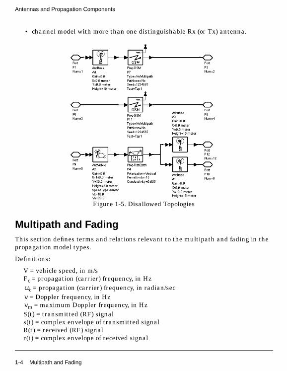
Figure 1-4 shows a Tx antenna output entering two channels, each connected to anRx antenna. This topology is used for simulation of antenna diversity or interference.

Figure 1-3. AWGN Noise Source

Figure 1-4. Tx Antenna Output

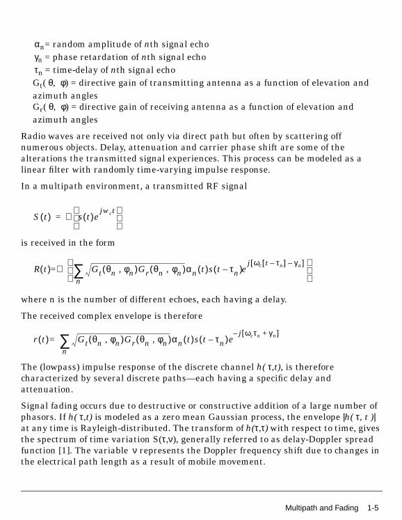
Figure 1-5 depicts the topologies that are not allowed; these include:

• channel model without Tx or Rx antenna

• channel model without Tx and Rx antenna

Introduction 1-3


• channel model with more than one distinguishable Rx (or Tx) antenna.

Figure 1-5. Disallowed Topologies

Multipath and FadingThis section defines terms and relations relevant to the multipath and fading in thepropagation model types.

Definitions:

V = vehicle speed, in m/sFc = propagation (carrier) frequency, in Hzωc = propagation (carrier) frequency, in radian/secν = Doppler frequency, in Hzνm = maximum Doppler frequency, in HzS(t) = transmitted (RF) signals(t) = complex envelope of transmitted signalR(t) = received (RF) signalr(t) = complex envelope of received signal

1-4 Multipath and Fading

αn= random amplitude of nth signal echoγn = phase retardation of nth signal echoτn = time-delay of nth signal echoGt( θ, φ) = directive gain of transmitting antenna as a function of elevation andazimuth anglesGr( θ, φ) = directive gain of receiving antenna as a function of elevation andazimuth angles

Radio waves are received not only via direct path but often by scattering offnumerous objects. Delay, attenuation and carrier phase shift are some of thealterations the transmitted signal experiences. This process can be modeled as alinear filter with randomly time-varying impulse response.

In a multipath environment, a transmitted RF signal

is received in the form

where n is the number of different echoes, each having a delay.

The received complex envelope is therefore

The (lowpass) impulse response of the discrete channel h( τ,t), is thereforecharacterized by several discrete paths—each having a specific delay andattenuation.

Signal fading occurs due to destructive or constructive addition of a large number ofphasors. If h( τ,t) is modeled as a zero mean Gaussian process, the envelope |h( τ, t )|at any time is Rayleigh-distributed. The transform of h(τ,τ) with respect to time, givesthe spectrum of time variation S(τ,ν), generally referred to as delay-Doppler spreadfunction [1]. The variable ν represents the Doppler frequency shift due to changes inthe electrical path length as a result of mobile movement.

S t( ) ℜ s t( )ejwct

=

R t( ) ℜ Gt θn , φn( )Gr θn , φn( )αn t( )s t τn–( )ej ωc t τn–[ ] γ n–[ ]

n∑

=

r t( ) Gt θn , φn( )Gr θn , φn( )αn t( )s t τn–( )ej ωcτn γn+[ ]–

n∑=

Multipath and Fading 1-5


For two vertically polarized transmit and receive antennas and horizontalpropagation of plane waves [2], the Doppler spectrum is

where

is the maximum Doppler shift due to vehicle speed. When a direct path exists thespectrum is Rician and is given by

with k1, k2, k3 constants related to proportion of direct and scattered signal and thedirect wave angle of arrival. Assuming the wide sense stationary uncorrelatedscattering (WSSUS) [3], the average delay profiles and Doppler spectra informationis needed for the simulation of radio channel. Delay profiles [4] P( τ) can be measured(or approximated) as

where

is the power associated with each path.

Assuming a uniform distribution of independent scatterers in the horizontal plane,each with a Doppler shift relative to the velocity of the mobile, the delay-Dopplerspread function S(τ, ν) and the impulse response of the channel can be constructed. Awide-band, frequency selective, multipath fading model can therefore be constructedusing a tapped-delay-line filter. The typical tapped-delay-line filter model forsimulation is illustrated in Figure 1-6.

S ν( ) 1

2πνm 1ν

νm-------

2–

--------------------------------------------- ν νm≤=

0= ν νm>

νmVc---- f c=

S ν( )k1

2πνm 1ν

νm-------

2–

--------------------------------------------- k2δ ν k3νm–( ) ν νm≤+=

P τ( ) σn2 δ τ τn–( )

n∑=

σn2

1-6 Multipath and Fading

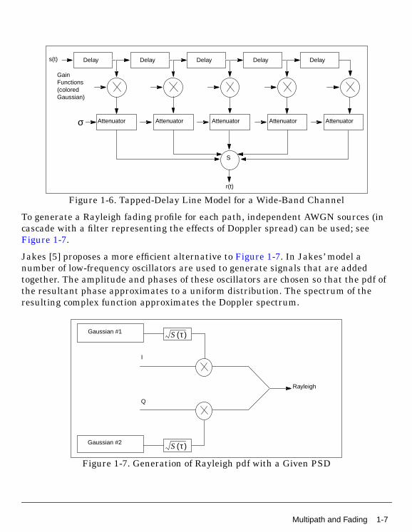
Figure 1-6. Tapped-Delay Line Model for a Wide-Band Channel

To generate a Rayleigh fading profile for each path, independent AWGN sources (incascade with a filter representing the effects of Doppler spread) can be used; seeFigure 1-7.

Jakes [5] proposes a more efficient alternative to Figure 1-7. In Jakes’ model anumber of low-frequency oscillators are used to generate signals that are addedtogether. The amplitude and phases of these oscillators are chosen so that the pdf ofthe resultant phase approximates to a uniform distribution. The spectrum of theresulting complex function approximates the Doppler spectrum.

Figure 1-7. Generation of Rayleigh pdf with a Given PSD

Delay

Attenuator

DelayDelay Delay Delays(t)

GainFunctions(coloredGaussian)

σ

S

r(t)

Attenuator Attenuator Attenuator Attenuator

Gaussian #1

Gaussian #2

I

Q

Rayleigh

S τ( )

S τ( )

Multipath and Fading 1-7


PathlossThis section defines terms and relations relevant to the pathloss in the propagationmodel types.

Definitions:

LFS = pathloss in free-space environment, in dBLRA = pathloss in rural area environment, in dBLHT = pathloss in hilly terrain environment, in dBLTU = pathloss in typical urban environment, in dBLTS = pathloss in typical suburban environment, in dBfc = propagation (carrier) frequency, in MHzλc = wavelength associated with propagation (carrier) frequency

D = major antenna dimensionHBS = base station antenna height, in metersHMS = mobile station antenna height, in metersR = distance between transmit and receive antenna, in kma = correction factor, in dB

Free-space pathloss option provides the user with an optimistic model. This option isgiven (in dB) by

LFS = + 20log10fc + 20log10R + 32.4

There are a wide variety of pathloss models—the most widely used is Hata’s. Hata’spathloss model [6] is based on an extensive data base derived by Okumura [7] frommeasurements in and around Tokyo. Hata’s pathloss models cover urban, rural, andsuburban environments and include the transmit and receive antenna heights.

The typical urban Hata model is given by

LTU = 69.55 + 26.16log10fc − 13.82log10HBS − a (HMS)+ (44.9 − 6.55log10HBS)log10R

The correction factor for small- to medium-size cities is given by

a = (1.1log10 fc − 0.7)HMS − (1.56 log10 fc − 0.8)

Hata’s urban model is equivalent to Type=TU in propagation components.

The typical suburban Hata model is given in terms of LTU with a correction factor:

1-8 Pathloss

LTS = LTU − 2[log10(fc/28)]2 − 5.4

Similarly, the rural Hata model is a corrected form of LTU as

LRA = LTU − 4.78(log10fc)2 + 18.33log10fc − 40.94

Hata’s rural model is equivalent to Type=RA in propagation components.

For GSM Hilly Terrain (HT) environment, adjustments prescribed in [5] are used.

All the pathloss formulas are valid—assuming that the receiving antenna is in thefar field of the transmit antenna. The common criterion for antennas whose physicalsize is in the order of wavelength is that path length should exceed D2/ λc.

References[1]J. D. Parsons, The Mobile Radio Propagation Channel, Halsted Press, 1992.

[2] R. H. Clarke, “A Statistical Theory of Mobile-Radio Reception”, The Bell SystemTechnical Journal, July-August 1968.

[3] Raymond Steele, Mobile Radio Communications, Pentech Press, 1992.

[4] GSM 05.05 Recommendation, Radio Transmission and Reception.

[5] W. C. Jakes (Editor), Microwave Mobile Communications, John Wiley & Sons,1974.

[6] M. Hata, “Empirical Formula for Propagation Loss in Land Mobile Radio”,IEEE Trans. VT-29, pp. 317-325, August 1980.

[7] Y. Okumura, “Field Strength and its Variability in VHF and UHF Land MobileService,” Review of Electrical Communication Laboratory, Vol 16, pp. 825-873,Sep-Oct. 1968.

References 1-9


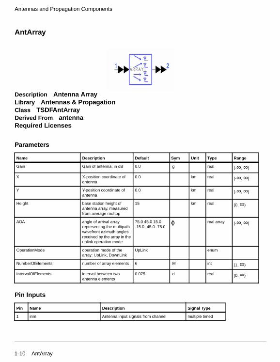
AntArray

Description Antenna ArrayLibrary Antennas & PropagationClass TSDFAntArrayDerived From antennaRequired Licenses

Parameters

Pin Inputs

Name Description Default Sym Unit Type Range

Gain Gain of antenna, in dB 0.0 g real (-∞, ∞)

X X-position coordinate ofantenna

0.0 km real (-∞, ∞)

Y Y-position coordinate ofantenna

0.0 km real (-∞, ∞)

Height base station height ofantenna array, measuredfrom average rooftop

15 km real (0, ∞)

AOA angle of arrival arrayrepresenting the multipathwavefront azimuth anglesreceived by the array in theuplink operation mode

75.0 45.0 15.0-15.0 -45.0 -75.0

ϕ real array (-∞, ∞)

OperationMode operation mode of thearray: UpLink, DownLink

UpLink enum

NumberOfElements number of array elements 6 M int (1, ∞)

IntervalOfElements interval between twoantenna elements

0.075 d real (0, ∞)

Pin Name Description Signal Type

1 inm Antenna input signals from channel multiple timed

1-10 AntArray

Pin Outputs

Notes/Equations

1. This component simulates an antenna array using gain of antenna and theangle of arrival of each multipath echo specified by the AOA parameter.

In the uplink mode, set by the OperationMode parameter, the model receives Linput timed signals from a multipath channel, processes these signals andoutputs M timed signal associated with an M-element array.

In the downlink mode, it sums all received input timed signals and transmits Mtimed signals corresponding to the M-element array.

At each firing, one timed token is consumed, and one token is produced.

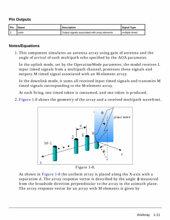
2. Figure 1-8 shows the geometry of the array and a received multipath wavefront.

Figure 1-8.

As shown in Figure 1-8 the uniform array is placed along the X-axis with aseparation d. The array response vector is described by the angle ϕ measuredfrom the broadside direction perpendicular to the array in the azimuth plane.The array response vector for an array with M elements is given by


2 outm Output signals associated with array elements multiple timed

AntArray 1-11


where

β = 2π/λ is the wavenumber

The output of element k of the array can be expressed as

where Xl is the lth multipath echo received by the array.

α ϕ l( )

1

jβd ϕl( )sin–( )exp

jβ2d ϕl( )sin–( )exp

...

jβ M 1–( )d ϕl( )sin–( )exp

=

yk g α ϕ kl( )Xll 1=

L

∑=

1-12 AntArray

AntBase

Description Base Station Stationary Antenna ModelLibrary Antennas & PropagationClass TSDFAntBaseDerived From antennaRequired Licenses

Parameters

Pin Inputs

Pin Outputs

Notes/Equations

1. Base (or fixed) station antennas are linearly polarized antennas used in mobilecommunication service at the base station of a radio relay link. Thespecification “EIA/TIA-329-B, Minimum Standards for Communication



X X-position coordinate 0.0 km real

Y Y-position coordinate 0.0 km real

Height antenna height above X-Yplane

10 km real (0, ∞)


1 input Antenna input signal multiple timed


2 output Antenna output signal timed

AntBase 1-13


Antennas, Part I-Base Station Antennas” describes the standards for this classof antennas.

2. This component radiation has a dominant vertical component of the electricfield (Ez).

3. The Gain unit is in dB and is defined with reference to an isotropic source (dBi).To comply with communication antenna standards, a dBd (gain with respect toa half-wave dipole) should be used, which is 2.15 dB over isotropic.

4. To accommodate for specification of input impedance versus frequency, circuitsubnetworks can be created and co-simulated with the appropriate circuitsimulator.

5. The antenna has a multi-input pin to receive multiple channels when at Rxmode. All inputs to AntBase must have the same carrier frequency.

6. For general information, refer to “Introduction” on page 1-1.

1-14 AntBase

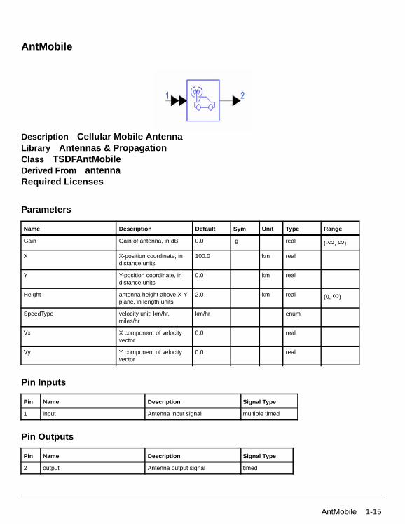
AntMobile

Description Cellular Mobile AntennaLibrary Antennas & PropagationClass TSDFAntMobileDerived From antennaRequired Licenses

Parameters

Pin Inputs

Pin Outputs



X X-position coordinate, indistance units

100.0 km real

Y Y-position coordinate, indistance units

0.0 km real

Height antenna height above X-Yplane, in length units

2.0 km real (0, ∞)

SpeedType velocity unit: km/hr,miles/hr

km/hr enum

Vx X component of velocityvector

0.0 real

Vy Y component of velocityvector

0.0 real


1 input Antenna input signal multiple timed


2 output Antenna output signal timed

AntMobile 1-15


Notes/Equations

1. Mobile antennas are mounted on vehicles and used in the land-mobilecommunications services. The specification “EIA/TIA-329-B-1, MinimumStandards for Communication Antennas, Part II-Vehicular Antennas” describesthe standards for this class of antennas.

2. This component radiation has a dominant vertical component of the electricfield (Ez).

3. The Gain unit is in dB and is an isotropic source (dBi). To comply withstandards for communication antennas, a dBd (gain with respect to a half-wavedipole) should be used, which is 2.15 dB over isotropic.

4. To accommodate for specification of input impedance versus frequency, circuitsubnetworks can be created and co-simulated with the appropriate circuitsimulator.

5. The antenna has a multi-input pin to receive multiple channels when at Rxmode. All inputs to AntMobile must have the same carrier frequency.

6. The mobile antenna position changes from initial location along a straight lineduring simulation. The new coordinates are

X′ (t) = X(t) + Vx × tY′ (t) = Y(t) + Vy × t

7. Propagation pathloss is updated based on changing distance between transmitand receive antennas.


1-16 AntMobile

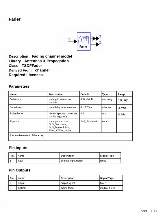
Fader

Description Fading channel modelLibrary Antennas & PropagationClass TSDFFaderDerived From channelRequired Licenses

Parameters

Pin Inputs

Pin Outputs

Name Description Default Type Range

GainArray path gain in terms ofdecible

0dB -10dB real array (-∞, ∞)†

DelayArray path delay in terms of ns 0ns 976ns int array [0, ∞)†

RicianFactor ratio of specular power andthe fading power

0.0 real [0, ∞)

Algorithm the algorithm used:SoS_Stochastic,SoS_Deterministic,Filter_AWGN_Noise

SoS_Stochastic enum

† for each element of the array


1 input channel input signal timed


2 output output signal timed

3 outChM fading factor multiple timed

Fader 1-17


Notes/Equations

1. This model is the fading channel emulator. The input signal is faded bymultiplying the fading coefficients generated using the selected algorithm. IfRicianFactor is 0.0, the fading probability density function is Rician distributed;otherwise the fading probability density function is Rayleigh distributed.

2. GainArray specifies the gain of each fading path in terms of decibel, while thedelay of each path is specified by DelayArray in terms of nanosecond. Thenumber of fading paths to be generated is equal to the size of GainArray andDelayArray. The generated multiple path fading coefficients are output frompin 3 for test purposes. Pin 2 is the output of the signal passing through amultipath fading channel.

3. The gain of this model has been normalized so that the output power is thesame as the input power regardless of the channel configuration. RicainFactoris the ratio of specular and fading power. The fading power is distributed to themultiple path signal according to the gain setting of each path. For example, ifthe input power is 1, RicianFactor is 2, and GainArray is “0dB -2dB”, then thespecular power will be 2/(1+2)=2/3 and fading power will be 1/(1+2)=1/3. Fadingpower allocated to path 1 will 0be

and power for path 2 will be

.

4. Three algorithms can be selected to generated the fading coefficient.

• stochastic sum-of-sinusoid method in which the number of oscillators areselected as 64[1];

• Jakes deterministic sum-of-sinusoid method [2];

• to pass an AWGN noise through a shaping filter; this filter is identical withthe one used in CDMA2K_ClassicSpec which is available in CDMA2K designlibrary.

5. This model is used in conjunction with antennas. Either a base station antennaor a mobile antenna is connected with the input and output pins. This model

13---

0.0 10⁄×10 100.0 10⁄ 10 2 10⁄–+( )⁄

13---

2 10⁄–×10 100.0 10⁄

102 10⁄–

+( )⁄

1-18 Fader

reads velocity information from the antenna to calculate the Doppler frequencyshift.

6. If the input time step is too large, interpolation will be performed to up-samplethe signal so that the resulted time step will be less than 1 nsec. Simulationtime in the case of a large interpolation rate would increase; in other caseswhen the delay for a path is larger, the signals to be buffered and interpolatedwould increase which would lead to increased simulation time.

7. If Filter_AWGN_Noise method is selected, it’s better to have the time step lessthan 1 µsec so that the fading coefficients will be more reasonable.

8. The fading coefficients generated by SoS_Stochastic and Filter_AWGN_Noisemethods are independent for different paths. However, caution must be given toproved [3] that the Jakes SoS Deterministic method doesn’t have goodcorrelation between different paths.


References

[1]Yahong R. Zheng and Chenshan Xiao, "Improved models for the generation ofmultiple un-correlated Rayleigh fading waveforms," IEEE CommunicationsLetters, vol. 6, no. 6, pp. 256-258, June 2002.

[2] W. C. Jakes, Microwave Mobile Communications: Wiley, 1974. Reprinted byIEEE Press in 1994.

[3] P. Dent, G. E. Bottomley, and T. Croft, "Jakes fading model revisited,"Electronics Letter, vol. 29, no. 13, pp. 1162-1163, June 1993.

Fader 1-19


PropFlatEarth

Description Direct and Reflected Ray Propagation ModelLibrary Antennas & PropagationClass TSDFPropFlatEarthDerived From channelRequired Licenses

Parameters

Pin Inputs

Pin Outputs

Notes/Equations

1. PropFlatEarth models the sum of a direct and reflected ray propagationchannel model based on polarization and flat earth properties.

2. This component is based on the two-ray LOS model where the received signal isthe sum of contributions from the direct and reflected rays. By summing the

Name Description Default Type

Polarization polarization type: Vertical,Horizontal

Vertical enum

Permittivity earth’s average relativepermittivity

15 real

Conductivity earth’s averageconductivity

0.005 real




2 output channel output signal timed

1-20 PropFlatEarth

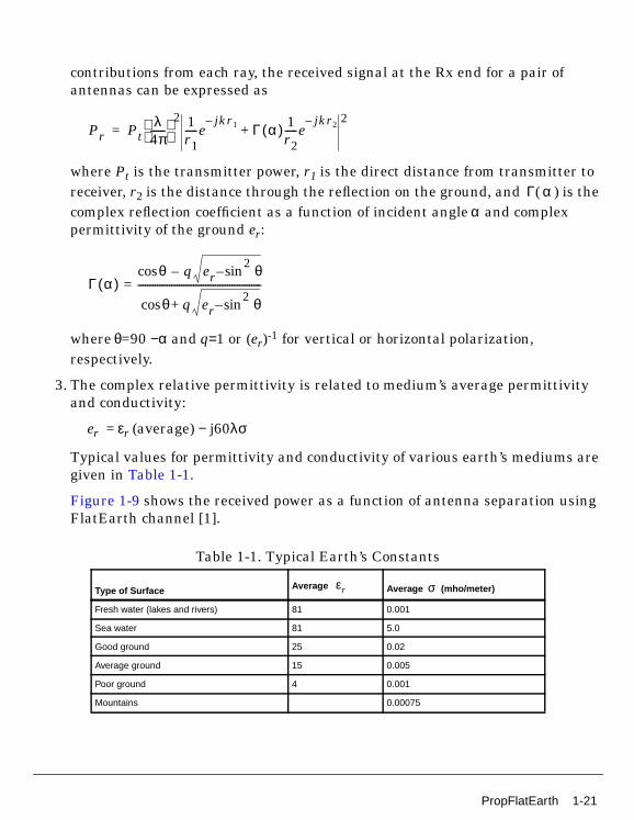
contributions from each ray, the received signal at the Rx end for a pair ofantennas can be expressed as

where Pt is the transmitter power, r1 is the direct distance from transmitter toreceiver, r2 is the distance through the reflection on the ground, and Γ( α ) is thecomplex reflection coefficient as a function of incident angle α and complexpermittivity of the ground er:

where θ=90 −α and q=1 or (er)-1 for vertical or horizontal polarization,respectively.

3. The complex relative permittivity is related to medium’s average permittivityand conductivity:

er = εr (average) − j60λσ

Typical values for permittivity and conductivity of various earth’s mediums aregiven in Table 1-1.

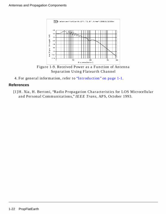
Figure 1-9 shows the received power as a function of antenna separation usingFlatEarth channel [1].

Table 1-1. Typical Earth’s Constants

Type of Surface Average Average (mho/meter)

Fresh water (lakes and rivers) 81 0.001

Sea water 81 5.0

Good ground 25 0.02

Average ground 15 0.005

Poor ground 4 0.001

Mountains 0.00075

Pr Ptλ

4π------

2 1r1-----e

jkr1–Γ α( ) 1

r2-----e

jkr2–+

2=

Γ α( )θ q er

2sin– θ–cos

θcos q er2

sin– θ+

---------------------------------------------------=

εr σ

PropFlatEarth 1-21


Figure 1-9. Received Power as a Function of AntennaSeparation Using Flatearth Channel


References

[1]H. Xia, H. Bertoni, “Radio Propagation Characteristics for LOS Microcellularand Personal Communications,” IEEE Trans, APS, October 1993.

1-22 PropFlatEarth

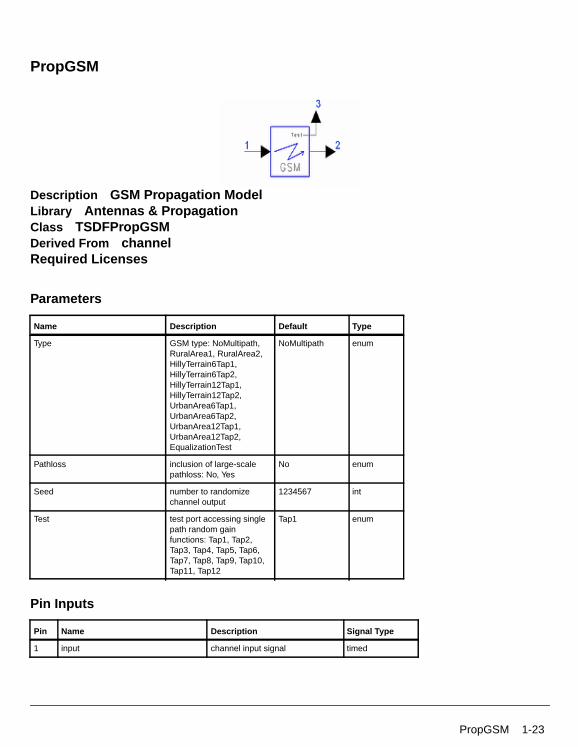
PropGSM

Description GSM Propagation ModelLibrary Antennas & PropagationClass TSDFPropGSMDerived From channelRequired Licenses

Parameters

Pin Inputs


Type GSM type: NoMultipath,RuralArea1, RuralArea2,HillyTerrain6Tap1,HillyTerrain6Tap2,HillyTerrain12Tap1,HillyTerrain12Tap2,UrbanArea6Tap1,UrbanArea6Tap2,UrbanArea12Tap1,UrbanArea12Tap2,EqualizationTest

NoMultipath enum

Pathloss inclusion of large-scalepathloss: No, Yes

No enum

Seed number to randomizechannel output

1234567 int

Test test port accessing singlepath random gainfunctions: Tap1, Tap2,Tap3, Tap4, Tap5, Tap6,Tap7, Tap8, Tap9, Tap10,Tap11, Tap12

Tap1 enum



PropGSM 1-23


Pin Outputs

Notes/Equations

1. PropGSM models a directional multipath channel based on GSM specifications.The model is a multi-tap filter, each tap having a delay and power. And, eachtap is modulated by a colored noise source (gain function).

Including the multipath fading and pathloss effects, the output of the channelcan be described as

where

α = pathloss attenuation, α≤1βi = relative power of each echo, per specificationτi = relative delay of each echo, plus the direct path delay τ0s(t) = complex envelope input signalgi = random gain function associated with each echo

For the NoMultipath option, M=1, τ1= τo

The gain function can be described as a sum of non-overlapping sinusoids ofequal amplitudes and different frequency and phases.

The pathloss attenuation factor α=1 when Pathloss=No. And, note that whenPathloss=No, the sum r(t) may add up to be more than the input s(t), implyingthat channel has a gain. For this reason, when Pathloss=No, the output isnormalized to the linear sum of echo powers with each option.

For more details, refer to “Introduction” on page 1-1.

2. The specification GSM 05.05, European Digital Cellular TelecommunicationsSystem (Phase 1) Radio Transmission and Reception, Annex 4 is the basis forthe PropGSM model. With the exception of Type= NoMultipath, which is anaddition, GSM system defines eleven different propagation profiles described by



3 test Test port timed

r t( ) α βis t τi–( )ejτ iωc–

gi t( )i 1=

M

∑

=

1-24 PropGSM

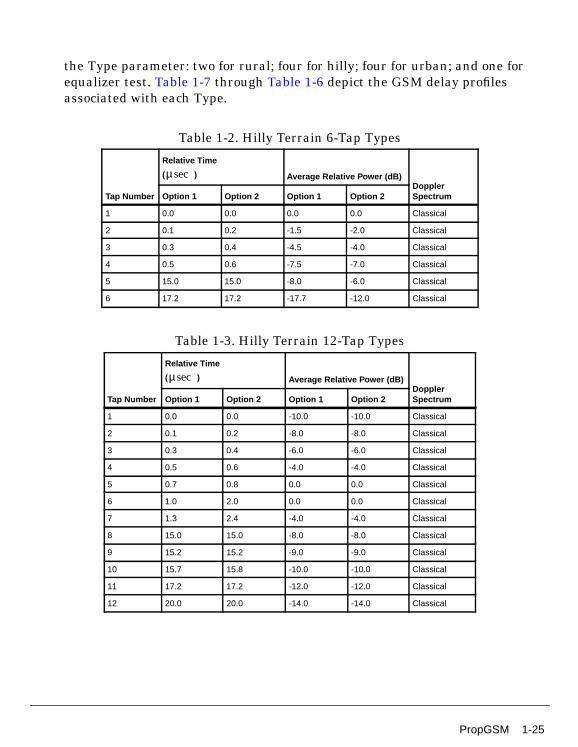
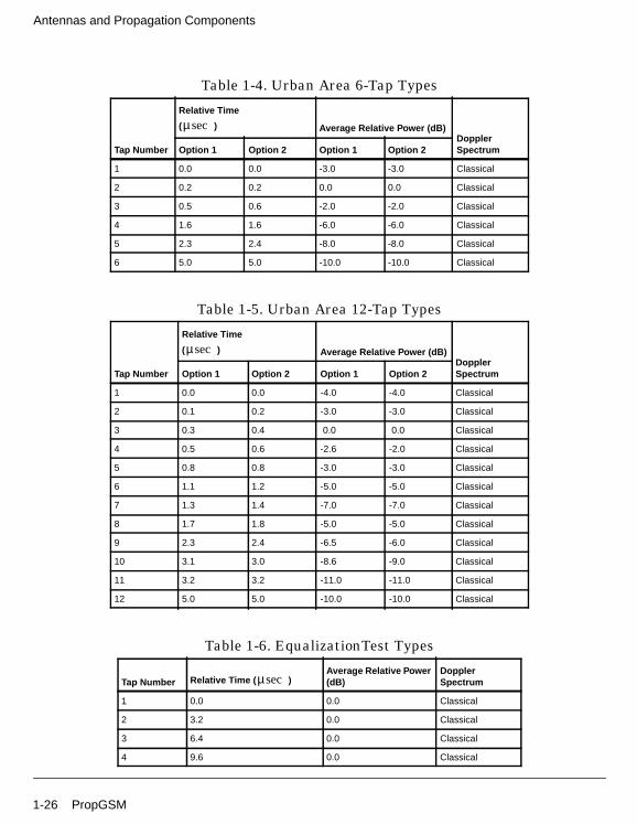
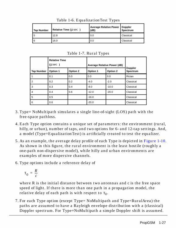
the Type parameter: two for rural; four for hilly; four for urban; and one forequalizer test. Table 1-7 through Table 1-6 depict the GSM delay profilesassociated with each Type.

Table 1-2. Hilly Terrain 6-Tap Types

Tap Number

Relative Time

( ) Average Relative Power (dB)DopplerSpectrumOption 1 Option 2 Option 1 Option 2

1 0.0 0.0 0.0 0.0 Classical

2 0.1 0.2 -1.5 -2.0 Classical

3 0.3 0.4 -4.5 -4.0 Classical

4 0.5 0.6 -7.5 -7.0 Classical

5 15.0 15.0 -8.0 -6.0 Classical

6 17.2 17.2 -17.7 -12.0 Classical

Table 1-3. Hilly Terrain 12-Tap Types

Tap Number

Relative Time


1 0.0 0.0 -10.0 -10.0 Classical

2 0.1 0.2 -8.0 -8.0 Classical

3 0.3 0.4 -6.0 -6.0 Classical

4 0.5 0.6 -4.0 -4.0 Classical

5 0.7 0.8 0.0 0.0 Classical

6 1.0 2.0 0.0 0.0 Classical

7 1.3 2.4 -4.0 -4.0 Classical

8 15.0 15.0 -8.0 -8.0 Classical

9 15.2 15.2 -9.0 -9.0 Classical

10 15.7 15.8 -10.0 -10.0 Classical

11 17.2 17.2 -12.0 -12.0 Classical

12 20.0 20.0 -14.0 -14.0 Classical

µ sec

µ sec

PropGSM 1-25


Table 1-4. Urban Area 6-Tap Types

Tap Number

Relative Time


1 0.0 0.0 -3.0 -3.0 Classical

2 0.2 0.2 0.0 0.0 Classical

3 0.5 0.6 -2.0 -2.0 Classical

4 1.6 1.6 -6.0 -6.0 Classical

5 2.3 2.4 -8.0 -8.0 Classical

6 5.0 5.0 -10.0 -10.0 Classical

Table 1-5. Urban Area 12-Tap Types

Tap Number

Relative Time


1 0.0 0.0 -4.0 -4.0 Classical

2 0.1 0.2 -3.0 -3.0 Classical

3 0.3 0.4 0.0 0.0 Classical

4 0.5 0.6 -2.6 -2.0 Classical

5 0.8 0.8 -3.0 -3.0 Classical

6 1.1 1.2 -5.0 -5.0 Classical

7 1.3 1.4 -7.0 -7.0 Classical

8 1.7 1.8 -5.0 -5.0 Classical

9 2.3 2.4 -6.5 -6.0 Classical

10 3.1 3.0 -8.6 -9.0 Classical

11 3.2 3.2 -11.0 -11.0 Classical

12 5.0 5.0 -10.0 -10.0 Classical

Table 1-6. EqualizationTest Types

Tap Number Relative Time ( )Average Relative Power(dB)

DopplerSpectrum

1 0.0 0.0 Classical

2 3.2 0.0 Classical

3 6.4 0.0 Classical

4 9.6 0.0 Classical

µ sec

µ sec

µ sec

1-26 PropGSM

3. Type= NoMultipath simulates a single line-of-sight (LOS) path with thefree-space pathloss.

4. Each Type option contains a unique set of parameters: the environment (rural,hilly, or urban), number of taps, and two options for 6- and 12-tap settings. And,a model (Type=EqualizationTest) is artificially created to test the equalizer.

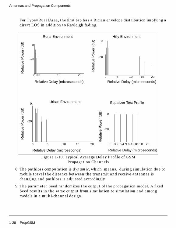
5. As an example, the average delay profile of each Type is depicted in Figure 1-10.As shown in this figure, the rural environment is the least hostile (roughly aone-path non-dispersive model), while hilly and urban environments areexamples of more dispersive channels.

6. Type options include a reference delay of

where R is the initial distance between two antennas and c is the free spacespeed of light. If there is more than one path in a propagation model, therelative delay of each path is with respect to τ0.

7. For each Type option (except Type= NoMultipath and Type=RuralArea) thepaths are assumed to have a Rayleigh envelope distribution with a (classical)Doppler spectrum. For Type=NoMultipath a simple Doppler shift is assumed.

5 12.8 0.0 Classical

6 16.0 0.0 Classical

Table 1-7. Rural Types

Tap Number

Relative Time


1 0.1 0.0 0.0 0.0 Rician

2 0.2 0.2 -4.0 -2.0 Classical

3 0.3 0.4 -8.0 -10.0 Classical

4 0.4 0.6 -12.0 -20.0 Classical

5 0.5 -16.0 Classical

6 0.6 -20.0 Classical

Table 1-6. EqualizationTest Types

Tap Number Relative Time ( )Average Relative Power(dB)

DopplerSpectrumµ sec

µ sec

τ0Rc----=

PropGSM 1-27


For Type=RuralArea, the first tap has a Rician envelope distribution implying adirect LOS in addition to Rayleigh fading.

Figure 1-10. Typical Average Delay Profile of GSMPropagation Channels

8. The pathloss computation is dynamic, which means, during simulation due tomobile travel the distance between the transmit and receive antennas ischanging and pathloss is adjusted accordingly.

9. The parameter Seed randomizes the output of the propagation model. A fixedSeed results in the same output from simulation to simulation and amongmodels in a multi-channel design.

Rural Environment

0

-20

10 20

Relative Delay (microseconds)

Rel

ativ

e P

ower

(dB

)

0.50

Hilly Environment

Rel

ativ

e P

ower

(dB

)


0

-20

0 6 10 15 20

Equalizer Test ProfileR

elat

ive

Pow

er (

dB)


0 3.2 6.4 9.6 12.816.0 20

-20

0

Urban Environment

Rel

ativ

e P

ower

(dB

)


0 5 10 15 20

-20

0

1-28 PropGSM

10. The test port is the output of a (user-selected) single path without pathloss ordelay effects. The output is the gain function, which is described in theintroductory part of this chapter.

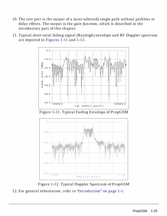
11. Typical short-term fading signal (Rayleigh) envelope and RF Doppler spectrumare depicted in Figures 1-11 and 1-12.

Figure 1-11. Typical Fading Envelope of PropGSM

Figure 1-12. Typical Doppler Spectrum of PropGSM


PropGSM 1-29


PropNADCcdma

Description Propagation Channel (CDMA) ModelLibrary Antennas & PropagationClass TSDFPropNADCcdmaDerived From channelRequired Licenses

Parameters

Pin Inputs

Pin Outputs


Type propagation type:NoMultipath, OnePath,TwoPath, ThreePath

NoMultipath enum

Pathloss inclusion of large scalepathloss: No, Yes

No enum

Env Environment Type Options:TypicalUrban,TypicalSuburban,RuralArea, FreeSpace

TypicalUrban enum

Seed number to randomizechannel output

1234567 int

Test test port for single pathrandom function: Tap1,Tap2, Tap3

Tap1 enum






1-30 PropNADCcdma

Notes/Equations

1. PropNADCcdma models a multipath channel based on IS-97 specifications. Themodel is a multi-tap filter, each tap having a delay and power. And, each tap ismodulated by a colored noise source.


where


For the NoMultipath option, M=1, τ1=τo



For more details, refer to the “Introduction” on page 1-1.

2. This component is based on the North American Dual Model Cellular (NADC)IS-97 specification.

3. Except for Type=NoMultipath, where free space pathloss and a pure Dopplershift is assumed, other Type options have a Rayleigh envelope distribution witha (classical) Doppler spectrum and pathloss defined by the Env parameter.

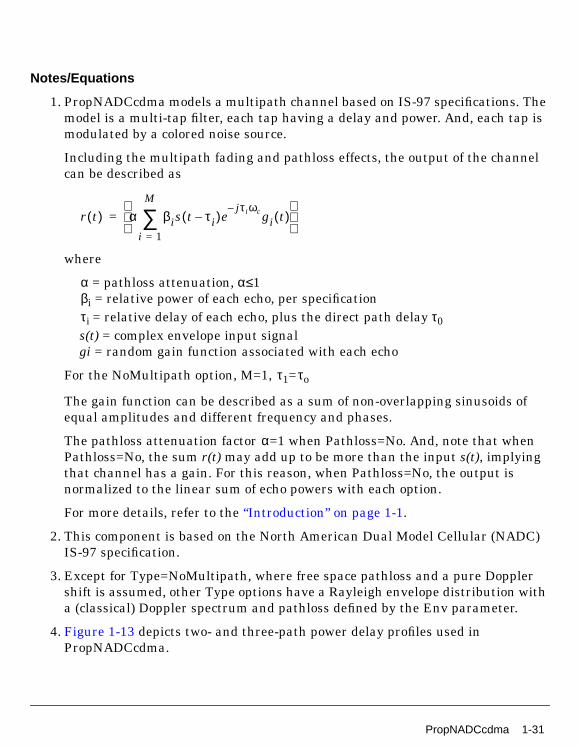
4. Figure 1-13 depicts two- and three-path power delay profiles used inPropNADCcdma.


gi t( )i 1=

M

∑

=

PropNADCcdma 1-31


Figure 1-13. Average Delay Profiles of CDMA Propagation Channels


where R is the initial distance between two antennas and c is the free spacespeed of light. If there is more than one path in a propagation model, therelative delay of each path is with respect to τ0.

6. The two- and three-path models have a Rayleigh envelope distribution with a(classical) Doppler spectrum.


8. The test port is the output of a (user-selected) single path without pathloss ordelay effects. The output is the gain function described in the introductory partof this chapter.

9. Sufficient simulation time is required for accurate pdf and cpdf. For evaluationof envelope statistics, it is preferable to have independent samples (that is,samples at a low rate, which implies TStep is large). The duration of thesimulation (Stop parameter of the data collecting sink) should be large enoughto cover 100 or more wavelengths of mobile travel.

CDMA Three-path

Rel

ativ

e P

ower

(dB

)

Relative Delay (microseconds)0 2 10.0 20

0

-3

14.5

CDMA Two-path

Rel

ativ

e P

ower

(dB

)Relative Delay (microseconds)

0

-3

0 2 10.0 20

τoRc----=

1-32 PropNADCcdma

This translates to simulation time that is greater than

where

is the maximum doppler frequency.

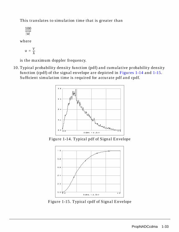
10. Typical probability density function (pdf) and cumulative probability densityfunction (cpdf) of the signal envelope are depicted in Figures 1-14 and 1-15.Sufficient simulation time is required for accurate pdf and cpdf.

Figure 1-14. Typical pdf of Signal Envelope

Figure 1-15. Typical cpdf of Signal Envelope

100υ

---------

υ Vλ----=

PropNADCcdma 1-33


PropNADCtdma

Description NADC Propagation (TDMA) Model, DirectionalLibrary Antennas & PropagationClass TSDFPropNADCtdmaDerived From channelRequired Licenses

Parameters

Pin Inputs


Type propagation type:NoMultipath, FlatFade,TwoPath

NoMultipath enum

Pathloss inclusion of large scalepathloss: No, Yes

No enum

Env Environment Type Options:TypicalUrban,TypicalSuburban,RuralArea, FreeSpace

TypicalUrban enum

Delay relative delay(Type=TwoPath) withrespect to first path, inmicroseconds

0.0 real

Pwr relative power(Type=TwoPath) withrespect to first path, in dB

0.0 real

Seed integer number torandomize channel output

1234567 int

Test test port for single path:Tap1, Tap2

Tap1 enum



1-34 PropNADCtdma

Pin Outputs

Notes/Equations

1. PropNADCtdma models a unidirectional multipath channel based on IS-55 andIS-56 propagation specifications. The model is a multi-tap filter, each tap havinga delay and power. And, each tap is modulated by a colored noise source gainfunction described in the introductory part of this chapter.


where


For the NoMultipath option, M=1, τ1=τ0 .



For more details, refer to the “Introduction” on page 1-1.

2. This component is based on the North American Dual Model Cellular (NADC).

3. Flat fade is assumed to be the non-frequency-selective fading.





gi t( )i 1=

M

∑

=

PropNADCtdma 1-35


4. Except for Type=NoMultipath where free space pathloss and a pure Dopplershift is assumed, all other Type options have a Rayleigh envelope distributionwith a (classical) Doppler spectrum and pathloss defined by the Env parameter.


where R is the initial distance between two antennas and c is the free spacespeed of light.

Delay in the two-ray model is the delay of the second ray with respect to thefirst ray, which is assumed to be τ0.

Pwr in the two-ray model is the power of the second ray below the power of thefirst ray.


7. The test port is the output of a (user-selected) single path without pathloss ordelay effects. The output is the gain function described in the introductory partof this chapter.

8. Typical envelope and envelope square spectrum of PropNADCtdma is shown inFigure 1-16. Also, pathloss profiles (no multipath) for different environmentsand different sets of transmit and receive antenna heights are shown inFigure 1-17.

τoRc----=

1-36 PropNADCtdma

Figure 1-16. Typical Envelope and Envelope Square Spectrumof PropNADCtdma

Figure 1-17. Pathloss Profiles for Different Environments

Envelope

Freespace

RuralSuburban

Urban

PropNADCtdma 1-37


PropWCDMA

Description WCDMA Propagation ChannelLibrary Antennas & PropagationClass TSDFPropWCDMADerived From channelRequired Licenses

Parameters

Pin Inputs

Name Description Default Sym Type Range

ChannelType Indicate the testenvironment ( Delay,Power, and DopplerSpectrum of each path ).:NoMultipath, Indoor A,Indoor B, Pedestrian A,Pedestrian B, Vehicular A,Vehicular B

Vehicular B enum

Pathloss option for inclusion oflarge-scale pathloss: No,Yes

No enum

Environment IMT2000 environment forpathloss computation:Indoor, Pedestrian,Vehicular, FreeSpace

FreeSpace enum

NumberOfFloors number of floors for indoorpathloss

4 int (0, ∞)

N 2N+1 is the number of sinewaves used in Jakes model

10 N int (0, ∞)

Seed integer number torandomize the channeloutput (Jakes model)

1234567 int (0, ∞)



1-38 PropWCDMA

Pin Outputs

Notes/Equations

1. This component models a fading channel based on the IMT2000 standardspecification. The specification includes the delay spread, doppler spread andpathloss for various environments. In addition to these, a line of sight (LOS)option called NoMultipath is available where the doppler shift due to mobilityand the LOS delay are modeled. The results are available at channel output pinmOut.

2. For doppler spread, Jakes model [2] is used which provides the dopplerspectrum as well as the statistics of the fading channel. An additional outputpin testOut is provided that conveys the complex gain multipliers of Jakesmodel.

3. The delay spread is modeled via a tap delay line where the number of taps isbased on the IMT2000 specifications for a given environment. There are 6options (A and B for indoor, pedestrian and vehicular environments) that aredepicted in Table 1-8 through Table 1-10. In each case the input signal isdelayed and the carrier phase due to the delay signal is incorporated. However,in the narrowband case (FLAT option in the indoor office test environment) onlythe carrier phase change associated with the multipath delay is included.

The modeling process is depicted in Figure 1-18, which indicates that theoutput of complex multipliers are summed. This is the case when PropWCDMAchannel is connected to a simple antenna. However, when the channel is notconnected to an array antenna, the output of complex multipliers are notsummed but each multipath (echo) acts like an independent wavefrontimpinging on the array elements (see WCDMAVectorChannel).

4. Unless stated otherwise, the use model is consistent with the guidelinesdescribed in the “Introduction” on page 1-1.

5. .The delay profile for the various channel types, summarized in Table 1-8through Table 1-10, result in the frequency selective fading.


2 testOut complex gain of the channel complex

3 mout Antenna input signal multiple timed

PropWCDMA 1-39


Table 1-8. Indoor Office Test Environment Tapped-Delay-Line Parameters

Tap

Channel A Channel B

DopplerSpectrum

Relative Delay(nSec) Avg. Power (dB)


1 0 0 0 0 FLAT

2 50 -3.0 100 -3.6 FLAT

3 110 -10.0 200 -7.2 FLAT

4 170 -18.0 300 -10.8 FLAT

5 290 -26.0 500 -18.0 FLAT

6 310 -32.0 700 -25.2 FLAT

Table 1-9. Outdoor to Indoor and Pedestrian Test EnvironmentTapped-Delay-Line Parameters

Tap

Channel A Channel B

Doppler SpectrumRelative Delay(nSec) Avg. Power (dB)


1 0 0 0 0 CLASSIC

2 110 -9.7 200 -0.9 CLASSIC

3 190 -19.2 800 -4.9 CLASSIC

4 410 -22.8 1200 -8.0 CLASSIC

5 2300 -7.8 CLASSIC

6 3700 -23.9 CLASSIC

Table 1-10. Vehicular Test Environment, High Antenna,Tapped-Delay-Line Parameters

Tap

Channel A Channel B

DopplerSpectrumRelative Delay (nSec) Avg. Power (dB)


1 0 0 0 -2.5 CLASSIC

2 310 -1.0 300 0 CLASSIC

3 710 -9.0 8900 -12.8 CLASSIC

4 1090 -10.0 12900 -10.0 CLASSIC

5 1730 -15.0 17100 -25.2 CLASSIC

6 2510 -20.0 20000 -16.0 CLASSIC

1-40 PropWCDMA

Figure 1-18. Delay and Doppler Spread and Carrier Phase Shift

References

[1]Draft New Recommendation ITU-R M.[FPLMT.REVAL], Guidelines forEvaluation of Radio Transmission Technologies for IMT-2000/FPLMTS(Question ITU-R 39/8).

[2] W. C. Jakes, Microwave Mobile Communications, IEEE Press, 1994.

Delay Delay Delay DelayDelay

Power

In

Out

Distribution

JakesModel

PropWCDMA 1-41


UserDefChannel

Description User-Defined ChannelLibrary Antennas & PropagationClass TSDFUserDefChannelDerived From channelRequired Licenses

Parameters

Pin Inputs


PathNumber number of multipath echos 2 L int (0, ∞)

AmpArray amplitude weight of patharray

1.0 0.5 real array (-∞, ∞)

DelayArray delays associated withpath array, inmicroseconds

0.1 0.2 real array (-∞, ∞)

Seed integer number torandomize channel output(Jakes model)

1234567 int (0, ∞)

N 2N+1 is number of sinewaves used in Jakes model

10 N int (0, ∞)


No enum

Env environment for pathlosscomputation: TypicalUrban,TypicalSuburban,RuralArea, FreeSpace

TypicalUrban enum



1-42 UserDefChannel

Pin Outputs

Notes/Equations

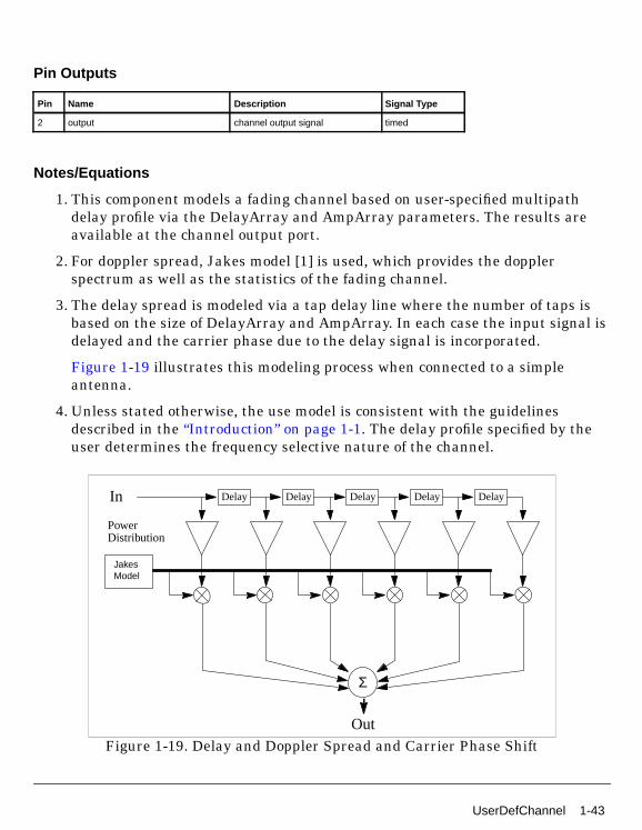
1. This component models a fading channel based on user-specified multipathdelay profile via the DelayArray and AmpArray parameters. The results areavailable at the channel output port.

2. For doppler spread, Jakes model [1] is used, which provides the dopplerspectrum as well as the statistics of the fading channel.

3. The delay spread is modeled via a tap delay line where the number of taps isbased on the size of DelayArray and AmpArray. In each case the input signal isdelayed and the carrier phase due to the delay signal is incorporated.

Figure 1-19 illustrates this modeling process when connected to a simpleantenna.

4. Unless stated otherwise, the use model is consistent with the guidelinesdescribed in the “Introduction” on page 1-1. The delay profile specified by theuser determines the frequency selective nature of the channel.

Figure 1-19. Delay and Doppler Spread and Carrier Phase Shift




JakesModel

Power

In

Out

Distribution

Σ

UserDefChannel 1-43


References

[1]W. C. Jakes, Microwave Mobile Communications, IEEE Press, 1994.

1-44 UserDefChannel

UserDefVectorChannel

Description User-Defined Vector ChannelLibrary Antennas & PropagationClass TSDFUserDefVectorChannelDerived From channelRequired Licenses

Parameters

Pin Inputs


PathNumber number of multipath echos 2 L int (0, ∞)

AmpArray amplitude weight of patharray

1.0 0.5 real array (-∞, ∞)

DelayArray delays associated withpath array, inmicroseconds

0.1 0.2 real array (-∞, ∞)

Seed integer number torandomize the channeloutput (Jakes model)

1234567 int (0, ∞)


10 N int (0, ∞)


No enum

Env environment for pathlosscomputation: TypicalUrban,TypicalSuburban,RuralArea, FreeSpace

TypicalUrban enum



UserDefVectorChannel 1-45


Pin Outputs

Notes/Equations

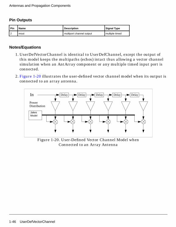
1. UserDefVectorChannel is identical to UserDefChannel, except the output ofthis model keeps the multipaths (echos) intact thus allowing a vector channelsimulation when an AntArray component or any multiple timed input port isconnected.

2. Figure 1-20 illustrates the user-defined vector channel model when its output isconnected to an array antenna.

Figure 1-20. User-Defined Vector Channel Model whenConnected to an Array Antenna


2 mout multiport channel output multiple timed


JakesModel

Power

In

Distribution

1-46 UserDefVectorChannel

WCDMAVectorChannel

Description WCDMA Vector ChannelLibrary Antennas & PropagationRequired Licenses

Parameters

Pin Inputs


ChannelType type of Channel:NoMultipath, Indoor A,Indoor B, Pedestrian A,Pedestrian B, Vehicular A,Vehicular B

Vehicular B enum

Echos number of multipath echos 6 L int (0, ∞)


No enum

Environment IMT2000 environment forpathloss computation:Indoor, Pedestrian,Vehicular, FreeSpace

FreeSpace enum

NumberOfFloors number of floors for indooroption

4 int (0, ∞)


10 N int (0, ∞)

Seed integer number torandomize the channeloutput(Jakes model)

1234567 int (0, ∞)


1 input channel input complex

WCDMAVectorChannel 1-47


Pin Outputs

Notes/Equations

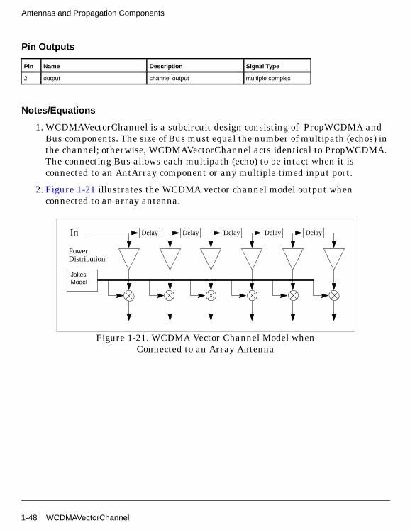
1. WCDMAVectorChannel is a subcircuit design consisting of PropWCDMA andBus components. The size of Bus must equal the number of multipath (echos) inthe channel; otherwise, WCDMAVectorChannel acts identical to PropWCDMA.The connecting Bus allows each multipath (echo) to be intact when it isconnected to an AntArray component or any multiple timed input port.

2. Figure 1-21 illustrates the WCDMA vector channel model output whenconnected to an array antenna.

Figure 1-21. WCDMA Vector Channel Model whenConnected to an Array Antenna


2 output channel output multiple complex


JakesModel

Power

In

Distribution

1-48 WCDMAVectorChannel

Index
AAntArray, 1-10AntBase, 1-13AntMobile, 1-15
FFader, 1-17

PPropFlatEarth, 1-20PropGSM, 1-23PropNADCcdma, 1-30PropNADCtdma, 1-34PropWCDMA, 1-38

UUserDefChannel, 1-42UserDefVectorChannel, 1-45

WWCDMAVectorChannel, 1-47

Index-1

Index-2

Antennas and Propagation Components -...

Documents

Transcript of Antennas and Propagation Components -...