Ant Colony Optimization Algorithms with Local Search...

Brock University

Department of Computer Science

Ant Colony Optimization Algorithms withLocal Search for the Dynamic Vehicle Routing

Problem

Andrew Runka

December 29, 2008

Advisor: Dr. Beatrice M. Ombuki-Berman

1

Abstract

This report demonstrates the use of effective local search to im-prove the performance of simple Ant Colony Optimization (ACO)algorithms as applied to an extension of the Vehicle Routing Problem(VRP) known as the Dynamic Vehicle Routing Problem (DVRP). Thestatic VRP presents all orders a priori, however the DVRP requiresscheduling to begin without a complete knowledge of all customer’s lo-cations, demands, and/or times. In recent years, much focus has beengiven to the study of meta-heuristics for use in solving static VRPs.Currently, however, emphasis is being put on DVRPs as they present abetter model with real-life applicability and challenges. The approachtaken in this paper is to model the DVRP as a series of static VRPs,and solve each one by applying the ACO meta-heuristic. Three simpleinstantiations of the ACO meta-heuristic are used, namely, the AntSystem (AS), the Ant Colony System (ACS), and the MAX-MIN AntSystem (MMAS). In order to make these simple algorithms effectivein such a difficult problem space, they are augmented with an inser-tion based local search, as well as a greedy step-based route scheduler.The algorithms are shown to outperform the only published ant-basedalgorithm for the DVRP model presented here, as well as achieve 4new best known results using publicly available benchmark probleminstances.

2

Acknowledgment

I would like to thank everyone who contributed to this project in every smallform. To all those who answered my many questions, to all those who guidedme to the answers, to all those who put up with me for the last year, and toall those who didn’t get to, Thank You!

More specifically I would like to thank Frank Hanshar for his willingnessto explain the smallest details, my friends and family for their continuedsupport, and of course my supervisor Dr. Ombuki-Berman without whomnone of this would have been possible.

3

Contents

1 Introduction 6

2 Background 82.1 Problem definition . . . . . . . . . . . . . . . . . . . . . . . . 8

2.1.1 Static Vehicle Routing Problem . . . . . . . . . . . . . 82.1.2 Dynamic Vehicle Routing Problem . . . . . . . . . . . 9

2.2 Ant Colony Optimization . . . . . . . . . . . . . . . . . . . . . 112.2.1 Ant Colony System . . . . . . . . . . . . . . . . . . . . 132.2.2 MAX-MIN Ant System . . . . . . . . . . . . . . . . . . 14

3 The ACO-DVRP algorithm 143.1 Event Handler . . . . . . . . . . . . . . . . . . . . . . . . . . . 143.2 ACO Module . . . . . . . . . . . . . . . . . . . . . . . . . . . 16

4 Experimental Setup and Discussion 174.1 Benchmark data . . . . . . . . . . . . . . . . . . . . . . . . . . 174.2 Experimental Setup . . . . . . . . . . . . . . . . . . . . . . . . 184.3 Results and Discussion . . . . . . . . . . . . . . . . . . . . . . 21

4.3.1 Local Search and Route Scheduler . . . . . . . . . . . . 214.3.2 Cloning vs. no cloning . . . . . . . . . . . . . . . . . . 224.3.3 Comparison of ant-based algorithms with local search

vs published ant based algorithm . . . . . . . . . . . . 254.3.4 Comparison of ant-based algorithms with local search

vs published GA and Tabu search . . . . . . . . . . . . 27

5 Conclusion 28

6 Appendix A 326.1 Tables of Results . . . . . . . . . . . . . . . . . . . . . . . . . 32

4

List of Figures

1 Sample DVRP routing scheme . . . . . . . . . . . . . . . . . . 112 ACO Meta-Heuristic Pseudo-code . . . . . . . . . . . . . . . . 123 ACO-DVRP structure diagram . . . . . . . . . . . . . . . . . 154 Event Handler Pseudo-code . . . . . . . . . . . . . . . . . . . 165 Distribution of customers . . . . . . . . . . . . . . . . . . . . . 196 Local Search vs Step Scheduler pressures . . . . . . . . . . . . 227 Cloning vs No cloning . . . . . . . . . . . . . . . . . . . . . . 24

List of Tables

1 ACO parameter settings . . . . . . . . . . . . . . . . . . . . . 202 DVRP parameter settings . . . . . . . . . . . . . . . . . . . . 203 AS with cloning vs. AS without cloning . . . . . . . . . . . . . 324 ACS with cloning vs ACS without cloning . . . . . . . . . . . 335 MMAS with cloning vs MMAS without cloning . . . . . . . . 346 AS vs ACS vs MMAS . . . . . . . . . . . . . . . . . . . . . . 357 AS clone vs Montemanni’s ACS . . . . . . . . . . . . . . . . . 368 AS no clone vs Montemanni’s ACS . . . . . . . . . . . . . . . 379 ACS clone vs Montemanni’s ACS . . . . . . . . . . . . . . . . 3810 ACS no clone vs Montemanni’s ACS . . . . . . . . . . . . . . 3911 MMAS clone vs Montemanni’s ACS . . . . . . . . . . . . . . . 4012 MMAS no clone vs Montemanni’s ACS . . . . . . . . . . . . . 4113 AS and ACS vs. [1]’s GA and Tabu . . . . . . . . . . . . . . . 42

5

1 Introduction

The Vehicle Routing Problem (VRP) is widely studied in the literature. Ithas been the subject of experimentation using a number of methods includ-ing several meta-heuristics such as Genetic Algorithms and Ant Colony Opti-mization (ACO). The VRP serves as an effective test-bed for many heuristicsdue to its complexity and wide variety of extensions. Also, this problem isNP-hard [2], and abstracts many real-world applications, especially in thefields of logistics and transportation.

The basic idea behind the VRP is that a fleet of vehicles, each with alimited capacity, are dispatched to service a set of customers. The objectivebeing to travel the shortest total distance with all vehicles in the process.The Dynamic Vehicle Routing Problem (DVRP) is an extension of the tra-ditional static VRP that has even more applicability to real world problems.The primary difference when extending the VRP to the DVRP is that thecustomers are not known in advance, but are revealed as the day progresses.Thus, the routes of the vehicles must adjust dynamically to accommodatenew customers. This more accurately reflects many real-world pickup or de-livery problems where not all customers are known prior to beginning theday. Larsen [3] describes a number of real-life applications of dynamic vehi-cle routing problems. Situations such as courier services, taxi services, andeven emergency services operate on a dynamic basis where the vehicles aredispatched without a complete schedule of stops. For this reason, focus isbeing shifted from the static VRP, where much research in the use of meta-heuristics has already been done, and is being placed on the DVRP.

Due to the dynamism, DVRPs are more difficult to solve than staticVRPs, and thus the use of approximation techniques has gained popularityfor such problems. To use an exact approach to find a solution to suchproblems is highly infeasible as the length of time required to find an exactsolution is likely much greater than the rate at which the problem stateis evolving. A number of meta-heuristics have been applied to variants ofDVRPs including tabu search [4, 5], and ACO [1, 6, 7].

Guntsch et al. [6] applied the ACO meta-heuristic to dynamic versions ofthe Traveling Salesman Problem (TSP) and the Quadratic Assignment Prob-lem. They used a modified ACO algorithm called FIFO-Queue ACO thatwas geared towards faster convergence in a dynamic environment. Eyckelhofet al. [7] augmented the simple Ant System (described in Section 2.2) witha novel pheromone control procedure known as ’shaking’. This was then ap-

6

plied to a dynamic TSP. Both of these papers report that traditional ACOalgorithms are capable of adapting to a dynamic environment, providing thatthe frequency of change or level of dynamism is low. The dynamic problemsin both papers are solved as single congruent and evolving problem.

Gambardella et al. [8] introduced a VRP-specific ACO variant knownas Multiple Ant Colony System (MACS). MACS uses two ant colonies tofirst minimize the number of vehicles and second to minimize the total traveltime. This approach proved to be effective in solving the Vehicle RoutingProblem with Time Windows (VRPTW), and is one of the top performingACO algorithms for the VRP to date. A survey of ACO algorithms appliedto VRPs is found in [9].

A number of DVRP variants exist, including those studied by Larsen[3], Gendreau et al. [10], Lund et al. [11], and Ichoua et al. [12]. TheDVRP variant employed in this report was originally proposed by Kilby etal. [13]. Montemanni et al.[1] then applied ACO to this DVRP providingthe first benchmark results based on meta-heuristics for this data. The spe-cific ACO implementation used in [1] is described as being “similar to theMACS-VRPTW algorithm”. In addition to creating benchmark results, [1]also introduces the “pheromone conservation procedure” for using ACO al-gorithms with the DVRP (described in 3.1). Following this, Hanshar et al.[14] applied a GA and simple Tabu search to this DVRP variant present-ing the majority of the currently best-known solutions for the DVRP modelintroduced in [13] and extended by [1].

This report aims at expanding the use of meta-heuristics, specificallyACO to the DVRP model discussed in [13], [1], and [14]. The main contri-bution of this report is two-fold. First, to study the effect of local search onstandard well-known ant-based algorithms. Secondly to further evaluate theuse of ant-based algorithms as applied to DVRPs.

The remainder of this report is structured as follows, Section 2 providesthe background on the DVRP model and ant-based algorithms studied here.Section 3 presents the details of the implemented ant-algorithms with localsearch. Section 4 provides the experimental setup and discusses the results.Finally, Section 5 presents the conclusions and future work.

7

2 Background

2.1 Problem definition

The DVRP variant considered in this report is based on the model firstproposed in [13], and later adopted by [1] and [14]. In this model, the DVRPis transformed into a series of static VRP instances. The static VRP canbe described as follows: A set of customers must be serviced by a fleet ofvehicles. Each customer has a specific amount of demand, and each vehiclecan only service a limited capacity of total demands. All customers mustbe serviced exactly once, and all vehicles must start and end their toursat a single depot. The objective is to find a routing scheme that describeswhich vehicles service which customers and in what order while minimizingthe total travel distance over all vehicles’ tours. The total travel distance isoften referred to as the total travel time, in this case there is an assumedconstant speed of one and thus they are equivalent.

2.1.1 Static Vehicle Routing Problem

The VRP can be represented mathematically as an undirected weightedgraph G = (V,A), where V = {v0,v1,...,vn} is a set of nodes representingthe depot (v0) and the set of customers (v1,...,vn), and A = {vi,vj |vi,vj ∈V} is a set of weighted arcs fully connecting V, which represent the traveltime/distance between customers. In addition, a homogenous set of m ve-hicles are used to service all customers exactly once. Each customer i isassociated with a demand qi, and each vehicle is associated with a capacityQ. A tour remains feasible if

∑qi ≤ Q remains true for all customers i ser-

viced by a given vehicle. The cost of any given solution can be calculatedas

Cost(Solution) =m∑j=0

k∑i=0

disti,i+1 (1)

where k is the size of route j, and disti,j is the distance between vi and vjor the weight along arci,j. Thus the objective is to find a solution whichminimizes the cost function while maintaining feasibility.

8

2.1.2 Dynamic Vehicle Routing Problem

Dynamic vehicle routing is a generic term that refers to vehicle routing andscheduling in a dynamic environment as opposed to a static one. Many spe-cific variants incorporate dynamism in terms of variable customer demands,variable arc weights between customers (simulating traffic levels), customerlocations, etc. The main difference between the DVRP model studied hereand the static VRP is that in the VRP all orders are known before any rout-ing takes place, whereas in the DVRP routing begins on a small set of knownorders, and as the day progresses new orders arrive which must also be accom-modated into the routing scheme. This is accomplished by means of dividingthe problem into a series of discrete time slices, each of which behaves simi-lar to a static VRP instance. Kilby et al. [13], originally proposed that thealgorithm run in real-time, that is, the length of the simulated working daywould be equivalent to the actual working day. In such a case, a given timeslice would stop when a new order arrived, and a new time slice would beginthat would include the new order. Montemanni et al. [1] however, decidedto maintain reasonable execution times for their simulations by limiting thetotal execution time to 1500 seconds or 25 minutes per working day. Theworking day was then divided into 25 equal time slices of one minute each.Hanshar et al. [14] later shortened this down to 30 seconds per time slice,due to implementation on a faster machine. In this case, all orders receivedduring the execution of one time slice are collected until the beginning of thenext time slice. They are then added to the list of serviceable customers. Inthis report, simulated timing is used as in [14].

A discrepancy arises between the simulated length of the working dayTsim and the actual duration of execution, which shall be denoted Treal.Every instance of the DVRP is associated with its own Tsim value. This isthe simulated length of the working day. It is mapped to a real-time valueby limiting the execution time of each time slice to Treal / nts, where ntsis the number of times slices. Similarly, each time slice is associated withsimulated and real-time values. For expressiveness we adopt the conventionthat all time values are simulated unless otherwise stated. Thus T and Tts

will refer to the simulated length of the working day and simulated length ofthe time slice respectively, while Treal and Ttsreal

will refer to their real-timeequivalents.

In each time slice, a given customer may be in one of three states:

1. not serviceable, not included in the routing scheme,

9

2. serviceable, position in routing scheme is not fixed, or

3. committed, position in the routing scheme is fixed.

All customers are associated with an availability. That is, the time in whichthey become serviceable. Initially, a subset of the customers, those knowna priori, are considered serviceable. These customers are considered to havecarried over from the previous working day. The cutoff time or Tco is the pointin the working day after which any new customers are postponed until thefollowing day. That is, customers with an availability greater than T · 0.5 arepostponed for processing. It has been adopted that these cutoff customers areused as the a priori customers for the given day. The remaining customers,those not known a priori, are initially considered not serviceable.

Each time slice works by generating a tentative routing scheme. That is,it generates a routing scheme on the assumption that the system as a wholewill remain unchanged until the end of the working day. This tentative rout-ing scheme is improved during each time slice by permuting the order ofserviceable customers. Each customer is associated with a given commit-ment time. This is the planned time during execution that the customer willbe serviced. If the commitment time of a customer in the tentative routingscheme occurs within the next time slice, then that customer becomes com-mitted and is no longer mutable starting from that time slice. A parameter,Tac, known as the advanced commitment time or commitment horizon, isintroduced as a buffer for the commitment of customers. Vehicles must haveTac advanced notice before committing customers. In practice, this meansthat all customers within the next Tts + Tac are committed. Committedcustomers hold static positions in the tentative routing schemes of each sub-sequent time slice. Any improvements on the routing scheme are consideredto start from the last committed customer on each route.

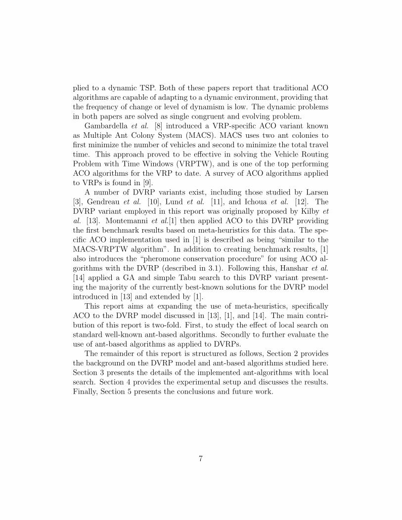
An example of a DVRP scheduling and routing in progress is illustratedby Figure 1 as depicted in [14]. This shows a snapshot of the tentativerouting scheme, with a number of committed customers (those connected to”completed route segments”), and a number of serviceable customers (thoseconnected by ”planned route segments”). Note that the arrival of a newrequest causes an alteration to the planned segments of a route.

10

New route segmentPlanned route segmentCompleted route segment

Immediate or new requestKnown request

Depot

Figure 1: Sample DVRP routing scheme

2.2 Ant Colony Optimization

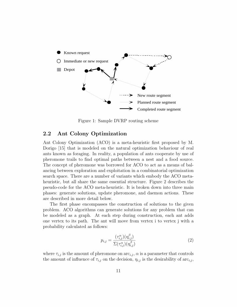
Ant Colony Optimization (ACO) is a meta-heuristic first proposed by M.Dorigo [15] that is modeled on the natural optimization behaviour of realants known as foraging. In reality, a population of ants cooperate by use ofpheromone trails to find optimal paths between a nest and a food source.The concept of pheromone was borrowed for ACO to act as a means of bal-ancing between exploration and exploitation in a combinatorial optimizationsearch space. There are a number of variants which embody the ACO meta-heuristic, but all share the same essential structure. Figure 2 describes thepseudo-code for the ACO meta-heuristic. It is broken down into three mainphases: generate solutions, update pheromone, and daemon actions. Theseare described in more detail below.

The first phase encompasses the construction of solutions to the givenproblem. ACO algorithms can generate solutions for any problem that canbe modeled as a graph. At each step during construction, each ant addsone vertex to its path. The ant will move from vertex i to vertex j with aprobability calculated as follows:

pi,j =(ταi,j)(η

βi,j)

Σ(ταi,j)(ηβi,j)

(2)

where τi,j is the amount of pheromone on arci,j, α is a parameter that controlsthe amount of influence of τi,j on the decision, ηi,j is the desirability of arci,j,

11

procedure ACO MetaHeuristicwhile(not termination)

GenerateSolutions()UpdatePheromone()DaemonActions()

end whileend procedure

Figure 2: ACO Meta-Heuristic Pseudo-code

which is some problem specific knowledge (e.g. 1disti,j

for the VRP), finally

β is the control parameter for ηi,j. This formula allows for the stochasticconstruction of a tour. At each state, an ant can choose between exploitationof a priori desirability information and a posteriori pheromone information,while maintaining the potential to explore less desirable solutions.

Once a population of solutions has been generated, the second phase,known as pheromone update, takes place. This phase is typically wherethe ACO variants differ. The discussion here pertains to the simplest ACOalgorithm known as Ant System (AS). The pheromone update can be sepa-rated into two steps: evaporation and deposit. The first step, evaporation,is calculated as follows:

τi,j = (1− ρ)τi,j (3)

where τi,j is the amount of pheromone on arci,j and ρ is a parameter thatcontrols the amount of evaporation. This formula is applied globally to everyarc. The second step, deposit, is calculated for each ant, and typically takesthe form:

∆τ ki,j =

{1Ck, if ant travels arci,j

0, otherwise(4)

where Ck is the cost of the kth ant’s solution. As this is done for each antthe effect accumulates on the arcs, and thus the following holds true:

∆τi,j =m∑k=0

∆τ ki,j (5)

12

where m is the number of ants. The two aforementioned steps can thus becombined into the following pheromone update formula:

τi,j = (1− ρ)τi,j + ∆τi,j (6)

By iteratively applying Formula 6, the arcs which are part of good toursthrough the graph will become condensed with more pheromone while thepheromone on the arcs that are not part of good tours will become scarce.The pheromone deposit increases the likelihood of exploitation of known goodareas of search, while the pheromone evaporation maintains the potentialfor exploration of unknown areas of search. Thus the convergence of thealgorithm is gradual allowing for an effective search of the solution space.

The third phase of the ACO metaheuristic is daemon actions. This is abroad term referring to any post processing of the given solutions, such as alocal search operation. The daemon actions used in this report are describedin detail in Section 3. Next, two extensions of the AS algorithm are discussedin the following sections.

2.2.1 Ant Colony System

The Ant Colony System (ACS) was designed by Dorigo and Gambardella [16],as an improvement to the simple AS algorithm. It is still based upon theACO metaheuristic, yet boasts some key changes from the AS that enable amore effective optimization strategy. The first change is the ‘pseudo-randomproportional rule’ which states that with probability q0 at each decision step,an ant will select the arc that maximizes (2), and with probability (1-q0)will select an edge as sone in AS. This rule increases the ‘greediness’ orthe exploitation used in the ants’ decisions. The second change in the ACSalgorithm is the introduction of a local pheromone update rule. This rulestates that at each step an ant takes, it applies the following formula to thearc that it traversed:

τi,j = (1− φ)τi,j + φ · τ0 (7)

where φ is the local evaporation parameter, and τ0 is the initial pheromonevalue. By removing the pheromone on used arcs, this rule decreases thelikelihood of having repeat solutions for a given round of construction. Thisleads to a more explorative construction phase. The final change in ACS isthat the typical pheromone update rule is changed such that the pheromonedeposit is only performed by the ant with the best solution.

13

2.2.2 MAX-MIN Ant System

Another extension of the AS algorithm is the MAX-MIN Ant System (MMAS),designed by Stutzle and Hoos [17]. This algorithm is named for its mostnotable contribution, maximum and minimum pheromone values. That is,MMAS introduces an explicit upper and lower bound on the amount ofpheromone possible on each arc. These bounds are controllable by the uservia parameters. A number of suggested formulas for computing these boundsare suggested in [17] and [18]. Here, we use the parameter ρDiff to repre-sent the inverse relative size of the gap between the upper and lower bounds.Thus, if ρDiff is large, then the gap is small. Also, similar to ACS, only thebest ant applies (6). Two final notes regarding MMAS: first, in the begin-ning all arcs are initialized to the maximum pheromone value. This createsa highly explorative initial search. Second, when the system approachesstagnation as determined by some criterion, all arcs are reinitialized to themaximum pheromone value.

3 The ACO-DVRP algorithm

The general approach used in this paper is inspired by those used in [1] and[14]. It can be broken down into two main components: The Event Handler,and the ACO module. The Event Handler controls the flow of the system;it manages all of the inputs and output from the user and coordinates thework done by the ACO module. The ACO module performs the execution ofan ACO algorithm to solve a given static VRP instance. The Event Handleris similar to that in [1] and [14]. The main contribution in this section isthe use of the three ACO algorithms which incarnate the ACO module. Thestructure of the system is illustrated in Figure 3 and described in more detailin Sections 3.1 and 3.2.

3.1 Event Handler

The Event Handler is responsible for subdividing the DVRP problem intoa series of time slices. Inherent in this task is the task of maintaining thestate of the dynamic system. That is, it must keep track of the currentsimulation time, the states of all customers, and the committed routes, aswell as the globally unchanging information such as the user’s parameters and

14

Figure 3: ACO-DVRP structure diagram

the problem instance. The pseudo-code for the event handler is presented inFigure 4.

The Event Handler begins by first initializing all of the data structures.Next, all those customers with availability times >Tco are assigned as theinitial pending orders. The event loop then begins, creating static problemsbased on the current state of the dynamic problem. These static problemsare then fed into the ACO Module which returns an optimized solution. Thesolution returned from the ACO Module is a tentative version of the routingscheme as described in Section 2. The Event Handler uses this routing schemeto update the current state of the dynamic problem. Essentially, any ordersthat have been serviced in the static routing scheme before the end of thenext time slice are considered committed. That is, their position in thedynamic routing scheme is fixed, and thus their position in all subsequentstatic problems is also fixed. The event loop continues until all customershave been committed and it is ensured that no more will arrive.

Another task for the Event Handler known as pheromone conservationwas introduced in [1]. The motivation for this task was that without it thepheromone matrix developed for one static problem would have no bearingon the next static problem, even though they are likely to be quite similar.The solution to this was to conserve a portion of the pheromone on eachedge from one time slice to the next. Pheromone conservation is achieved byapplying formula (8) to all arcs that appear in both the previous and current

15

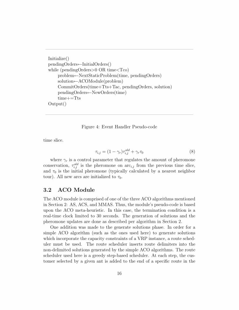
Initialize()pendingOrders←InitialOrders()while (pendingOrders>0 OR time<Tco)

problem←NextStaticProblem(time, pendingOrders)solution←ACOModule(problem)CommitOrders(time+Tts+Tac, pendingOrders, solution)pendingOrders←NewOrders(time)time+=Tts

Output()

Figure 4: Event Handler Pseudo-code

time slice.

τi,j = (1− γr)τ oldi,j + γrτ0 (8)

where γr is a control parameter that regulates the amount of pheromoneconservation, τ oldi,j is the pheromone on arci,j from the previous time slice,and τ0 is the initial pheromone (typically calculated by a nearest neighbortour). All new arcs are initialized to τ0.

3.2 ACO Module

The ACO module is comprised of one of the three ACO algorithms mentionedin Section 2: AS, ACS, and MMAS. Thus, the module’s pseudo-code is basedupon the ACO meta-heuristic. In this case, the termination condition is areal-time clock limited to 30 seconds. The generation of solutions and thepheromone updates are done as described per algorithm in Section 2.

One addition was made to the generate solutions phase. In order for asimple ACO algorithm (such as the ones used here) to generate solutionswhich incorporate the capacity constraints of a VRP instance, a route sched-uler must be used. The route scheduler inserts route delimiters into thenon-delimited solutions generated by the simple ACO algorithms. The routescheduler used here is a greedy step-based scheduler. At each step, the cus-tomer selected by a given ant is added to the end of a specific route in the

16

delimited routing scheme. The specific route in the scheme that it is addedto is selected as the one with the minimum distance between its last stopand the current customer. If adding to the selected route is invalid, then thenext best route is selected. If no valid routes are available, then a new routeis created and the customer is inserted there.

In terms of daemon actions, a local search was applied. The local searchused is an insertion technique based on the method of the Route Crossoverintroduced by Ombuki et al. [19] and further developed in [20] as the Best-Cost Route Crossover (BCRC). The BCRC is a crossover developed for usein VRP problems for the genetic algorithm meta-heuristic, however, it in-corporates a local search technique which is adopted here. Essentially, theuncommitted customers are each selected at random, removed from theircurrent positions, and reinserted into the location that generates the great-est decrease in total cost of the solution while maintaining the validity of thesolution.

One final modification in the ACO module was inspired by a conflictbetween the MMAS algorithm and the pheromone conservation procedure.At the beginning of execution of the MMAS algorithm the pheromone matrixis initialized to the maximum value. Thus there can be no carryover ofpheromone between time slices via the pheromone conservation procedure, asall such conservation would be erased at initialization. Thus, another methodof sharing good solutions between time slices was needed. The simplestmanner of doing so is to copy the solutions themselves (i.e. elitism/cloning).Simply put, at the end of each time slice, the best solution is already beingreported to the event handler for use in updating the dynamic problem. Thisprocedure simply has the event handler share this information with the nexttime slice. The ACO Module then utilizes this information, by initializingits best ant as the best ant from the previous time slice. Any new ordersare added to the best ant as one or more new routes as needed. The ACOmodule then continues as normal.

4 Experimental Setup and Discussion

4.1 Benchmark data

The instances used were created by modifying three sets of commonly usedVRP instances, namely Christofides [21], Fisher [22], and Taillard [23]. First

17

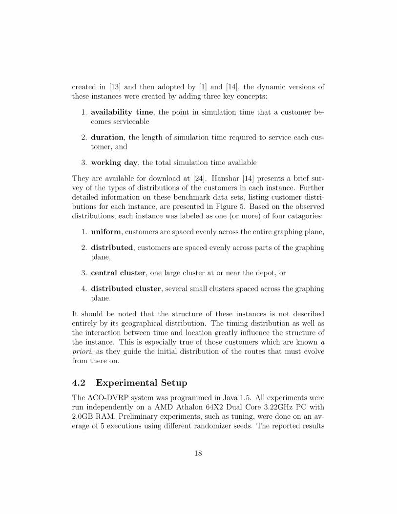
created in [13] and then adopted by [1] and [14], the dynamic versions ofthese instances were created by adding three key concepts:

1. availability time, the point in simulation time that a customer be-comes serviceable

2. duration, the length of simulation time required to service each cus-tomer, and

3. working day, the total simulation time available

They are available for download at [24]. Hanshar [14] presents a brief sur-vey of the types of distributions of the customers in each instance. Furtherdetailed information on these benchmark data sets, listing customer distri-butions for each instance, are presented in Figure 5. Based on the observeddistributions, each instance was labeled as one (or more) of four catagories:

1. uniform, customers are spaced evenly across the entire graphing plane,

2. distributed, customers are spaced evenly across parts of the graphingplane,

3. central cluster, one large cluster at or near the depot, or

4. distributed cluster, several small clusters spaced across the graphingplane.

It should be noted that the structure of these instances is not describedentirely by its geographical distribution. The timing distribution as well asthe interaction between time and location greatly influence the structure ofthe instance. This is especially true of those customers which are known apriori, as they guide the initial distribution of the routes that must evolvefrom there on.

4.2 Experimental Setup

The ACO-DVRP system was programmed in Java 1.5. All experiments wererun independently on a AMD Athalon 64X2 Dual Core 3.22GHz PC with2.0GB RAM. Preliminary experiments, such as tuning, were done on an av-erage of 5 executions using different randomizer seeds. The reported results

18

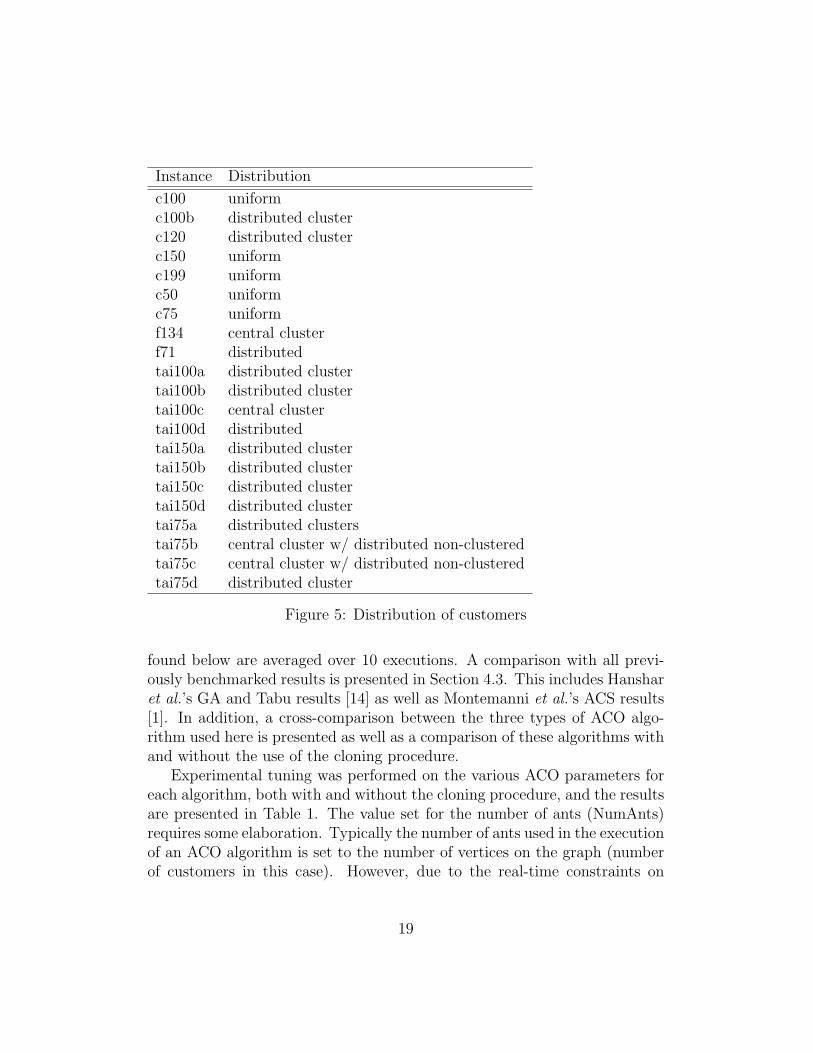
Instance Distribution

c100 uniformc100b distributed clusterc120 distributed clusterc150 uniformc199 uniformc50 uniformc75 uniformf134 central clusterf71 distributedtai100a distributed clustertai100b distributed clustertai100c central clustertai100d distributedtai150a distributed clustertai150b distributed clustertai150c distributed clustertai150d distributed clustertai75a distributed clusterstai75b central cluster w/ distributed non-clusteredtai75c central cluster w/ distributed non-clusteredtai75d distributed cluster

Figure 5: Distribution of customers

found below are averaged over 10 executions. A comparison with all previ-ously benchmarked results is presented in Section 4.3. This includes Hansharet al.’s GA and Tabu results [14] as well as Montemanni et al.’s ACS results[1]. In addition, a cross-comparison between the three types of ACO algo-rithm used here is presented as well as a comparison of these algorithms withand without the use of the cloning procedure.

Experimental tuning was performed on the various ACO parameters foreach algorithm, both with and without the cloning procedure, and the resultsare presented in Table 1. The value set for the number of ants (NumAnts)requires some elaboration. Typically the number of ants used in the executionof an ACO algorithm is set to the number of vertices on the graph (numberof customers in this case). However, due to the real-time constraints on

19

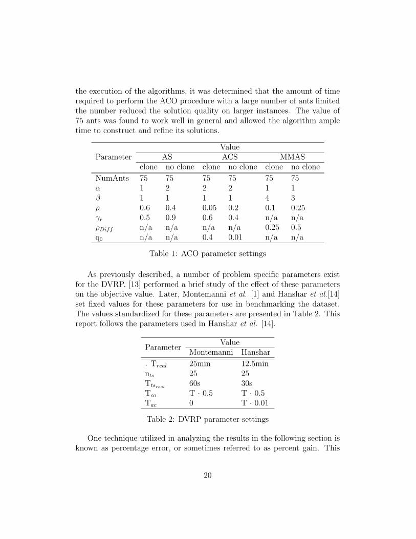
the execution of the algorithms, it was determined that the amount of timerequired to perform the ACO procedure with a large number of ants limitedthe number reduced the solution quality on larger instances. The value of75 ants was found to work well in general and allowed the algorithm ampletime to construct and refine its solutions.

ParameterValue

AS ACS MMASclone no clone clone no clone clone no clone

NumAnts 75 75 75 75 75 75α 1 2 2 2 1 1β 1 1 1 1 4 3ρ 0.6 0.4 0.05 0.2 0.1 0.25γr 0.5 0.9 0.6 0.4 n/a n/aρDiff n/a n/a n/a n/a 0.25 0.5q0 n/a n/a 0.4 0.01 n/a n/a

Table 1: ACO parameter settings

As previously described, a number of problem specific parameters existfor the DVRP. [13] performed a brief study of the effect of these parameterson the objective value. Later, Montemanni et al. [1] and Hanshar et al.[14]set fixed values for these parameters for use in benchmarking the dataset.The values standardized for these parameters are presented in Table 2. Thisreport follows the parameters used in Hanshar et al. [14].

ParameterValue

Montemanni Hanshar

. Treal 25min 12.5minnts 25 25Ttsreal

60s 30sTco T · 0.5 T · 0.5Tac 0 T · 0.01

Table 2: DVRP parameter settings

One technique utilized in analyzing the results in the following section isknown as percentage error, or sometimes referred to as percent gain. This

20

value yields a normalized and signed difference between two results as follows:

%error =Observed− Expected

Expected· 100 (9)

where Observed and Expected are the two values between which the error iscalculated. This yields a positive error if Observed is greater than Expectedand a negative error if it is less. In terms of the current minimization problem,a negative error refers to an increase in optimality.

This calculation is utilized in two ways in the following experiments. Theexperimental results are presented in tabular format comparing the perfor-mance of each algorithm against each other over 21 instances. At the bottomof each column is the averaged result, this is the sum of the respective columndivided by 21. The percent error is calculated on the average result as wellas for each instance. The latter produces a series of numbers which is thenaveraged to give an average percentage error.

4.3 Results and Discussion

4.3.1 Local Search and Route Scheduler

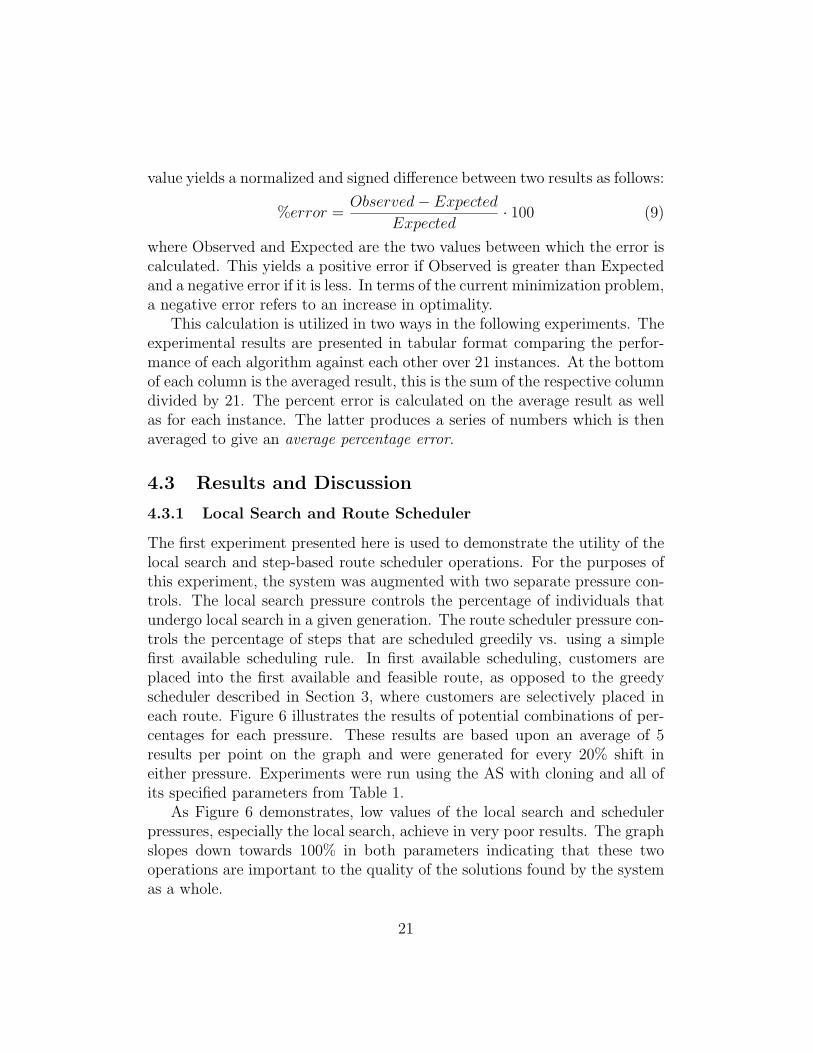
The first experiment presented here is used to demonstrate the utility of thelocal search and step-based route scheduler operations. For the purposes ofthis experiment, the system was augmented with two separate pressure con-trols. The local search pressure controls the percentage of individuals thatundergo local search in a given generation. The route scheduler pressure con-trols the percentage of steps that are scheduled greedily vs. using a simplefirst available scheduling rule. In first available scheduling, customers areplaced into the first available and feasible route, as opposed to the greedyscheduler described in Section 3, where customers are selectively placed ineach route. Figure 6 illustrates the results of potential combinations of per-centages for each pressure. These results are based upon an average of 5results per point on the graph and were generated for every 20% shift ineither pressure. Experiments were run using the AS with cloning and all ofits specified parameters from Table 1.

As Figure 6 demonstrates, low values of the local search and schedulerpressures, especially the local search, achieve in very poor results. The graphslopes down towards 100% in both parameters indicating that these twooperations are important to the quality of the solutions found by the systemas a whole.

21

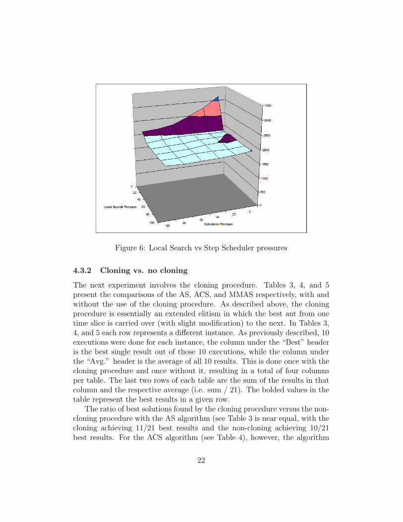
Figure 6: Local Search vs Step Scheduler pressures

4.3.2 Cloning vs. no cloning

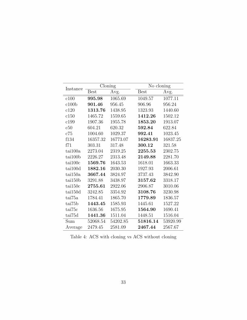
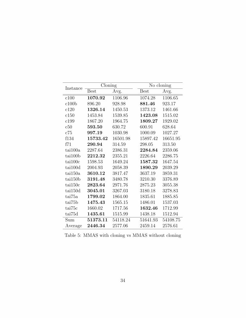
The next experiment involves the cloning procedure. Tables 3, 4, and 5present the comparisons of the AS, ACS, and MMAS respectively, with andwithout the use of the cloning procedure. As described above, the cloningprocedure is essentially an extended elitism in which the best ant from onetime slice is carried over (with slight modification) to the next. In Tables 3,4, and 5 each row represents a different instance. As previously described, 10executions were done for each instance, the column under the “Best” headeris the best single result out of those 10 executions, while the column underthe “Avg.” header is the average of all 10 results. This is done once with thecloning procedure and once without it, resulting in a total of four columnsper table. The last two rows of each table are the sum of the results in thatcolumn and the respective average (i.e. sum / 21). The bolded values in thetable represent the best results in a given row.

The ratio of best solutions found by the cloning procedure versus the non-cloning procedure with the AS algorithm (see Table 3 is near equal, with thecloning achieving 11/21 best results and the non-cloning achieving 10/21best results. For the ACS algorithm (see Table 4), however, the algorithm

22

without the cloning procedure outperforms the algorithm with the cloningprocedure, 12 to 9. A percentage error calculation of the summed averagedresults (last row from each table) using cloning as the expected and no cloningas the observed yields an error of +0.41% in favour of cloning for the ASand -0.49% in favour of no-cloning for the ACS. An averaged percent errorcalculation over all instances yields an error of -0.32% for the AS and -0.37%for the ACS, with a standard deviation of 2.1% and 2.9% respectively. Thusan advantage to either algorithm does exist from one instance to the next,however on average the algorithm without the cloning procedure performsvery slightly better for these two ACO variants.

The third ACO variant, the MMAS, was the original motivation for thecloning procedure. Recall that the other two ACO variants (AS and ACS)use the pheromone conservation procedure which performs a similar task asthe cloning procedure. Thus for the AS and the ACS, the cloning procedureis redundant. The MMAS on the other hand, initializes the pheromonematrix to the maximum pheromone value at each time slice, thus pheromoneconservation has no effect. So the cloning procedure is not redundant whenapplied to the MMAS. It is therefore expected that the MMAS algorithmwith the cloning procedure would out-perform the MMAS algorithm withoutthe cloning procedure with some significance. The optimal value ratio is infavour of this hypothesis, with 14/21 instances of the cloning outperformingthe non-cloning, a ratio of 2/3. However, the percentage error calculationusing the summed averaged results shows only a +0.52% error in favourof the cloning procedure. The average percentage error over all instancesis +0.24% with a standard deviation of 2.26%. Therefore, there is littleevidence to suggest a significant increase, although the MMAS with cloningprocedure does marginally outperform the non-cloning MMAS algorithm.

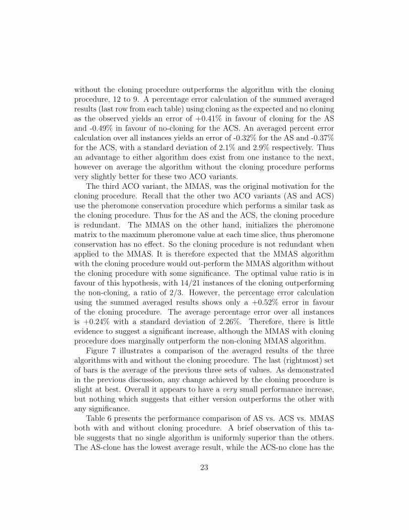
Figure 7 illustrates a comparison of the averaged results of the threealgorithms with and without the cloning procedure. The last (rightmost) setof bars is the average of the previous three sets of values. As demonstratedin the previous discussion, any change achieved by the cloning procedure isslight at best. Overall it appears to have a very small performance increase,but nothing which suggests that either version outperforms the other withany significance.

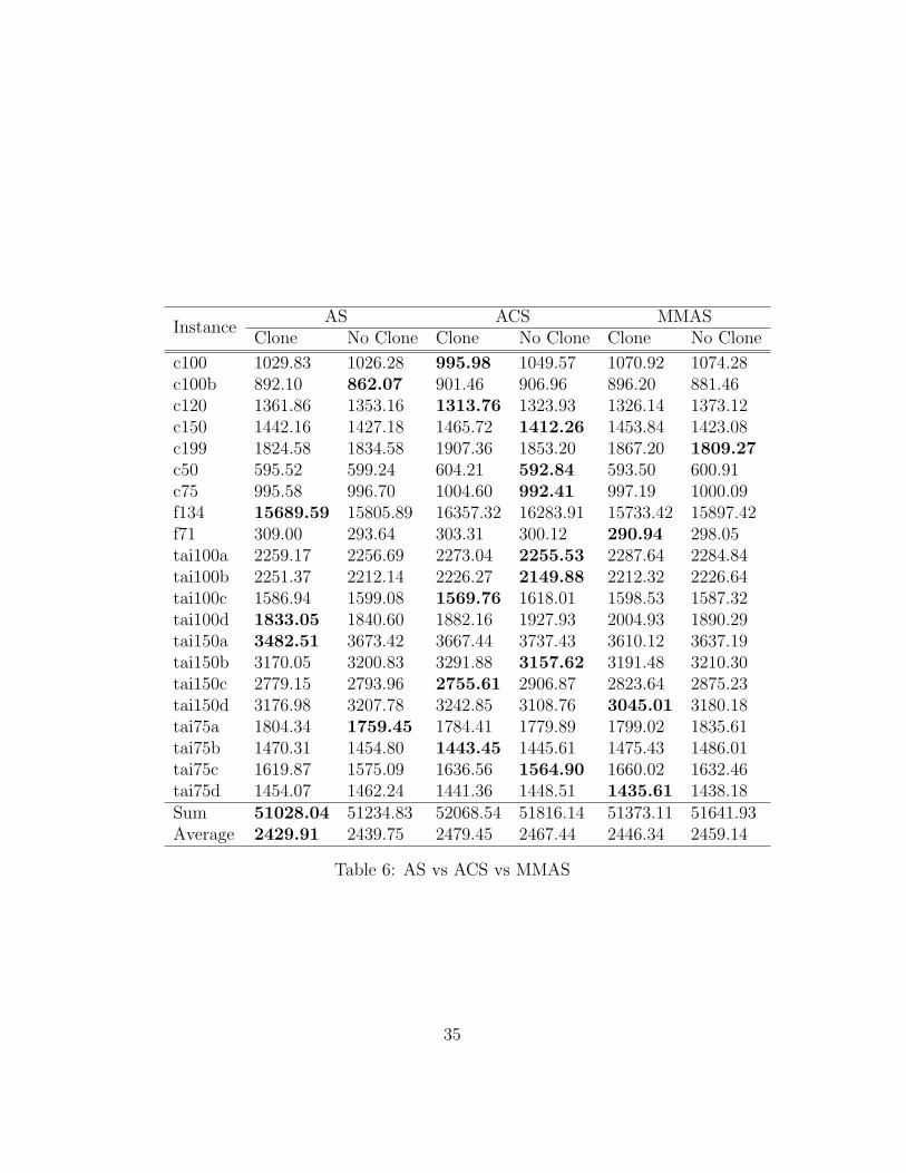
Table 6 presents the performance comparison of AS vs. ACS vs. MMASboth with and without cloning procedure. A brief observation of this ta-ble suggests that no single algorithm is uniformly superior than the others.The AS-clone has the lowest average result, while the ACS-no clone has the

23

Figure 7: Cloning vs No cloning

highest count of best results. On the other hand, the ACS-clone has thesecond highest count of best results as well as the worst average result. Apercentage error analysis of the summed average result of each algorithm wasperformed against the summed average result from the AS-clone algorithmand the following results were observed:

• AS-no clone: 0.41%,

• ACS-clone: 2.04%,

• ACS-no clone: 1.54%,

• MMAS-clone: 0.68%,

• MMAS-no clone: 1.20%.

This seems to suggest that the AS-clone algorithm outperforms the otheralgorithms. An average percentage error calculation was performed overall instances against the AS-clone results, and the following results wereobserved:

• AS-no clone: -0.32%, StDev: 2.10%,

24

• ACS-clone: 0.66%, StDev: 2.52%,

• ACS-no clone: 0.26%, StDev: 3.08%,

• MMAS-clone: 0.57%, StDev: 3.09%,

• MMAS-no clone: 0.76%, StDev: 1.98%.

AS-clone out performs most other algorithms with an average percentageerror of less than 1%. Such a small gap leaves much room for speculation.The relatively high standard deviations combined with the low average differ-ence implies that that the comparison is not one-sided, that each algorithmoutperforms the other over several instances each. This supports the initialobservation, that no single algorithm is uniformly superior.

4.3.3 Comparison of ant-based algorithms with local search vspublished ant based algorithm

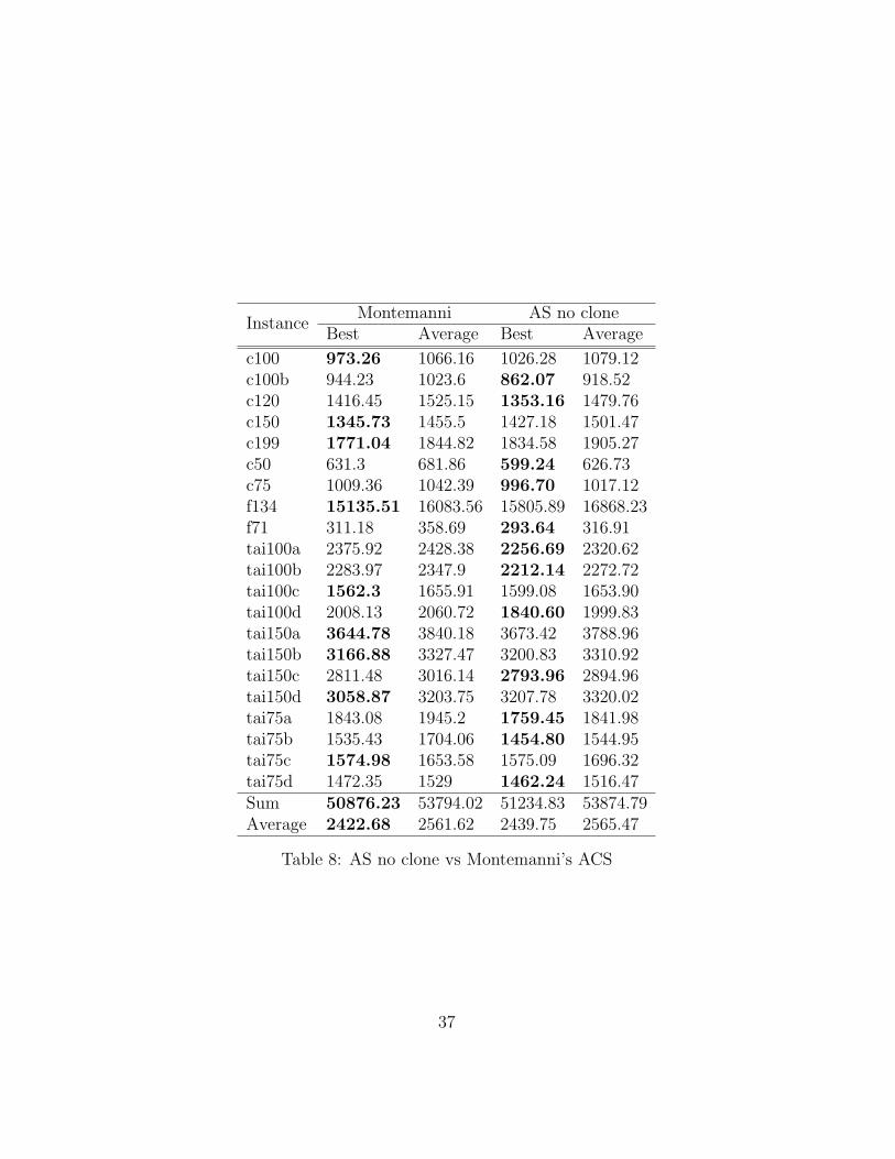
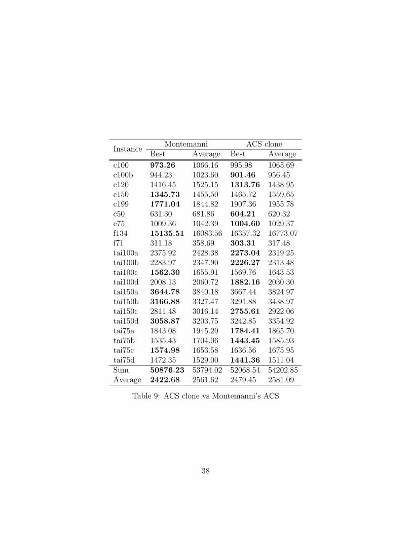
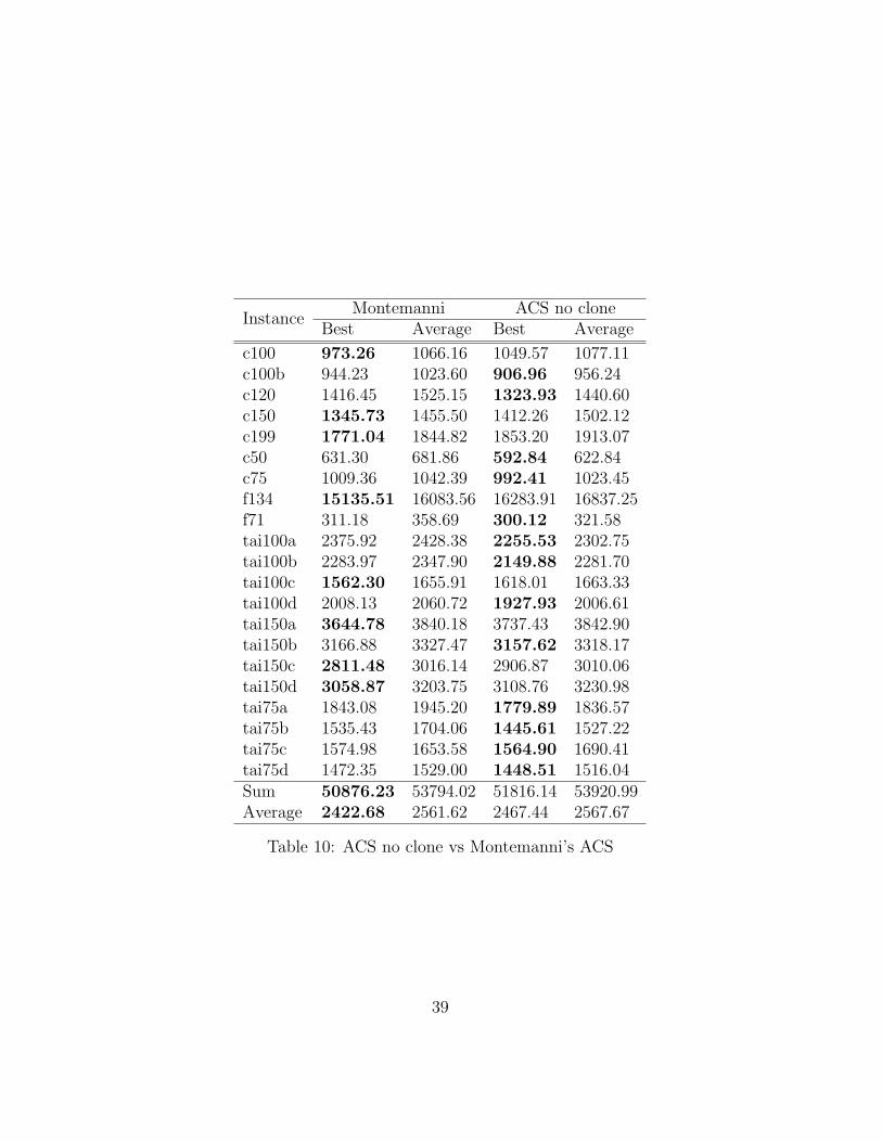
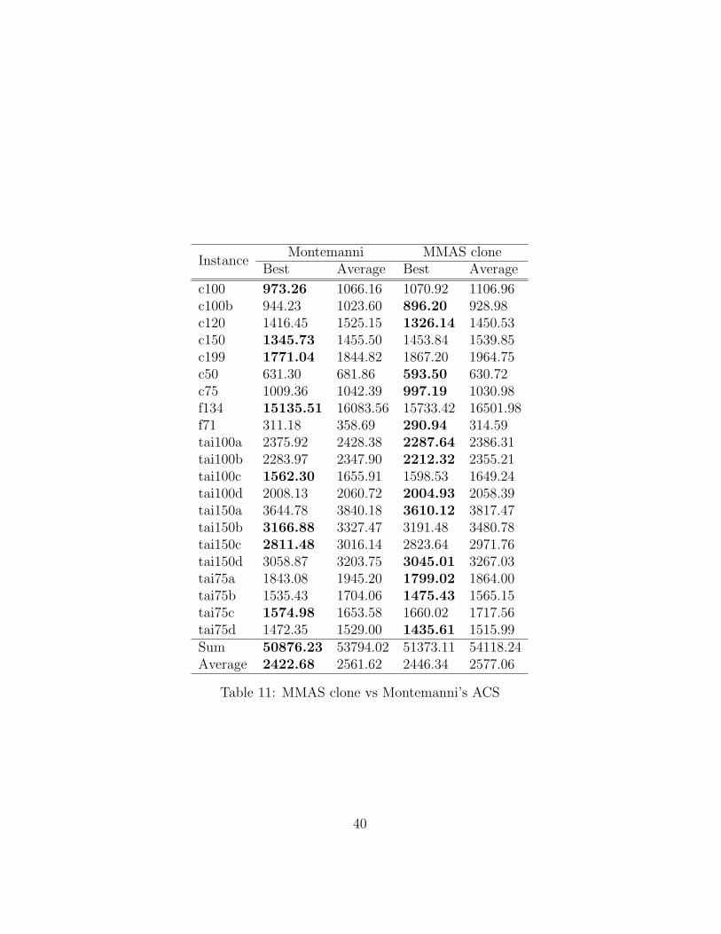
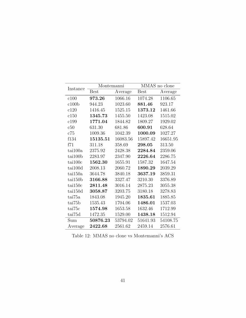
The next experiment compares the ACO algorithms from this study againstthe only pre-existing ACO results for the DVRP. Tables 7, 8, 9, 10, 11, and12 present comparisons between the various algorithms in this study and theresults from Montemanni et al. [1]. The results are broken into six tables, asthis gives a more accurate depiction of the ratio comparison between each ofthis study’s algorithms and Montemanni’s ACS. The ratio comparison is asimple count of the number of best results (highlighted in bold in each table)achieved by each algorithm out of the total number of instances. The resultsof this comparison are as follows:

• AS-clone: 13/21,

• AS-no clone: 12/21,

• ACS-clone: 12/21,

• ACS-no clone: 13/21,

• MMAS-clone: 13/21,

• MMAS-no clone: 12/21.

25

The ACO algorithms from this report achieve between 57% and 62% ofthe best solutions per comparison. Suggesting that these algorithms all havea slight advantage in performance over Montemanni’s ACS. At the time ofwriting this, the results found in [1] maintain only one best known result,the result for f134. A best-known result is one that is the best one foundthroughout all of the literature. The best-known result for f134 remainsunchanged as the ACO results from this paper were unable to achieve alower minimum for this instance.

By looking at each table it is clear that the summed average result fromMontemanni’s ACS is lower than that of every other algorithm in this com-parison. The percentage error calculation of each algorithm as compared toMontemanni’s ACS yields the following results:

• AS-clone: 0.30%

• AS-no clone: 0.70%

• ACS-clone: 2.34%

• ACS-no clone: 1.85%

• MMAS-clone: 0.98%

• MMAS-no clone: 1.51%

These percentages however, conflict with the following results retrievedvia an average percentage error calculation over all instances:

• AS-clone: -0.82%, StDev: 4.16%,

• AS-no clone: -1.15%, StDev: 4.53%,

• ACS-clone: -0.17%, StDev: 4.97%,

• ACS-no clone: -0.59%, StDev: 4.62%,

• MMAS-clone: -0.29%, StDev: 4.70%,

• MMAS-no clone: -0.09%, StDev: 4.34%.

26

The ACO algorithms from this study uniformly outperform Montemanni’sACS in terms of the ratio test as well as the average percentage errornumberof best results achieved as well as the average amount of error among thoseresults, while Montemanni’s ACS outperforms the ACO algorithms of thisstudy in terms of the average solution quality. It is worth mention, thatthe average solution quality is skewed by the larger instances more than thesmaller ones. As an example, the f134 instance, for which Montemanni’s ACSholds the best known result, has results that are approximately 50x largerthan the results of the c50. This means that a 1% difference in solutionquality for the f134 has about 50x more impact on the average solutionquality than a 1% difference in solution quality for the c50. This suggeststhat the averaged percentage error over each instance as well as the ratio ofbest solutions has more merit in terms of describing which algorithms aremore optimal than the average solution quality. For this reason it is assertedthat the results from this paper outperform those of Montemanni’s ACS.

4.3.4 Comparison of ant-based algorithms with local search vspublished GA and Tabu search

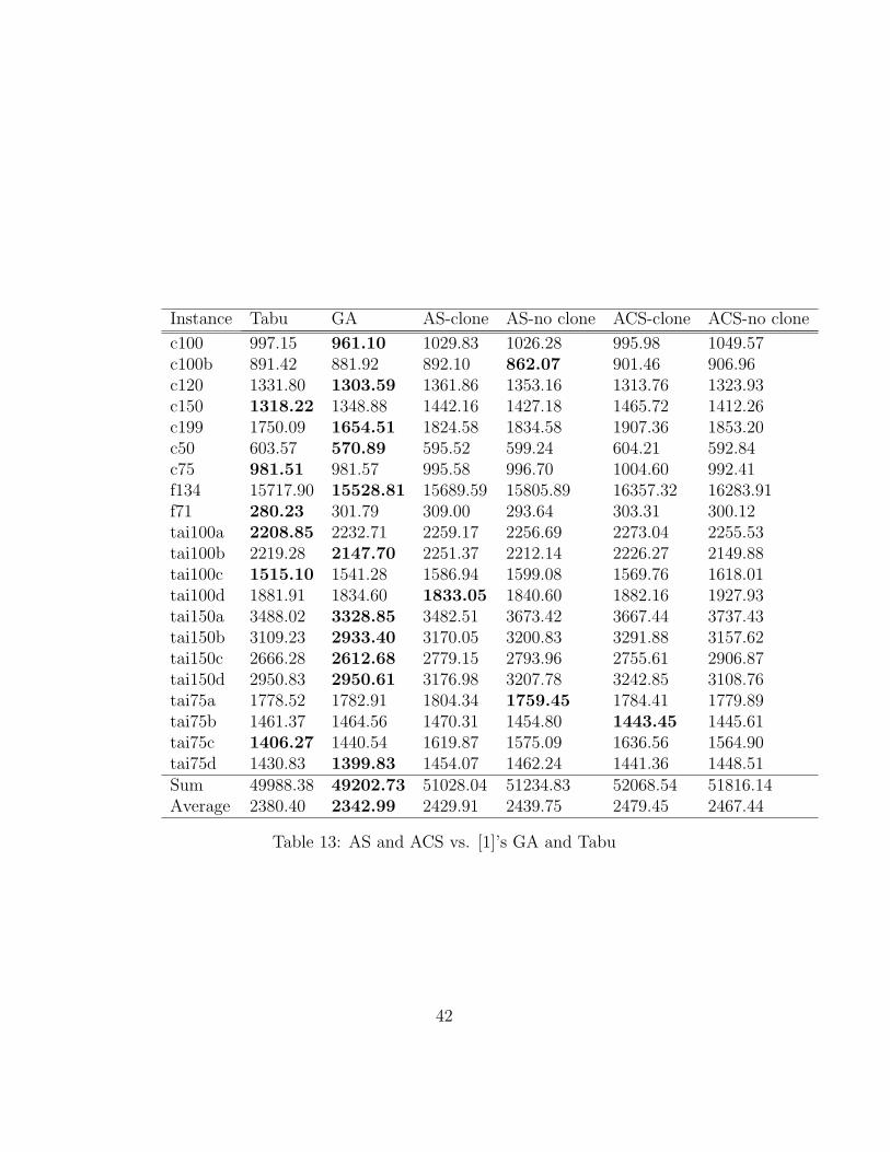
The final experiment in this report compares the results from this study tothose found by Hanshar et al. in [14]. [14] presents two algorithms, a Tabuand a GA, both of which are presented in Table 13 along side the results ofthis study. For display purposes the MMAS results are not presented as theycontributed little to this comparison. At the time this report was written, thetwo algorithms from [14] hold 20 out of 21 best known results. Therefore,all optimal values in Table 13 (highlighted in bold) represent best knownresults, with the exception of f134, which [1] has found the best result for.

A brief observation of Table 13 reveals that the algorithms developedin this study have achieved four new best known results. The averagedpercentage error for all instances between the GA and each algorithm is asfollows:

• AS-clone: 4.41%, StDev: 3.43%,

• AS-no clone: 4.08%, StDev: 4.20%,

• ACS-clone: 5.12%, StDev: 4.74%,

• ACS-no clone: 4.66%, StDev: 4.18%.

27

These figures clearly illustrate the dominance of the GA results over theant-based results from this study.

5 Conclusion

This report has studied the application of three of the simplest and wellknown Ant Colony Optimization algorithms to the Dynamic Vehicle routingproblem. By applying a simple insertion local search and greedy step-basedroute scheduler, the performance of the ACO algorithms was improved. Thisreport also analyzed the application of a cloning procedure to the ant-basedalgorithms and found it to offer minimal improvement. A comparison of thealgorithms presented here with the only available published ACO algorithmfor this variant of DVRP proved that the local searches had made a greatimpact on the quality of the simple ACO algorithms, allowing problem non-specific algorithms to perform competitively. Although the improvementsby the local search on the ACO algorithms lead to an improvement of thenumber of best solutions as compared to the currently available ACO workfor the DVRP, the improvement was not sufficient to out-perform the solutionquality by GA and Tabu. In this regard, further work is needed in the ant-based algorithms for the DVRP to better compete with GA and Tabu search.Four new best known results were discovered amongst the 21 instances.

Potential future work should focus on developing insight about the struc-ture of the instances themselves. This would aid in the development ofalgorithms that are better suited for coping with the dynamic nature of thedynamic vehicle routing problem. In addition to this, there are other po-tential variants of DVRP which, if studied, could garner some benefit to thereal-world industry.

28

References

[1] R. Montemanni, L. Gambardella, A. Rizzoli, and A. Donati, “Ant colonysystem for a dynamic vehicle routing problem,” Journal of Combinato-rial Optimization, vol. 10, pp. 327–343, June 2005.

[2] M. R. Garey and D. S. Johnson, Computers and Intractability A Guideto the Theory of NP-Completeness. Murray Hill, New Jersey: BellLaboratories, 1979.

[3] A. Larsen, “The dynamic vehicle routing problem,” Ph.D. dissertation,Technical University of Denmark, 2000.

[4] M. Gendreau, F. Guertin, J.-Y. Potvin, and E. Talliard, “Parallel tabutsearch for real-time vehicle routing and dispatching,” TransportationScience, vol. 33, no. 4, pp. 381–390, 1999.

[5] M. Gendreau, G. Laporte, and R. Seguin, “A tabu search heuristic forthe vehicle routing problem with stochastic demands and customers,”Operations Research, vol. 44, pp. 469–477, 1996.

[6] M. Guntsch and M. Middendorf, “Applying population based aco todynamic optimization problems,” in ANTS ’02: Proceedings of the ThirdInternational Workshop on Ant Algorithms. London, UK: Springer-Verlag, 2002, pp. 111–122.

[7] C. Eyeckelhof and M. Snoek, “Ant systems for a dynamic tsp,” inANTS ’02: Proceedings of the Third International Workshop on AntAlgorithms. London, UK: Springer-Verlag, 2002, pp. 88–99.

[8] L. M. Gambardella, E. Taillard, and G. Agazzi, “Macs-vrptw: A multi-ple ant colony system for vehicle routing problems with time windows,”IDSIA, Tech. Rep., 1999.

[9] A. Rizzoli, F. Oliverio, R. Montemanni, and L. Gambardella, “Antcolony optimization for vehicle routing problems: from theory to ap-plications,” IDSIA, Tech. Rep., 2004.

[10] M. Gendreau and J. yves Potvin, “Dynamic vehicle routing and dis-patching,” Fleet Management and Logistics, pp. 115 – 126, 1998.

29

[11] K. Lund, O. B. G. Madsen, and J. M. Rygaard, “Vehicle routing prob-lems with varying degrees of dynamism,” IMM, The Department ofMathematical Modelling, Technical University of Denmark, Tech. Rep.,1996.

[12] S. Ichoua, M. Gendreau, and J.-Y. Potvin, “Diversion issues in real-timevehicle dispatching,” Transportation Science, vol. 34, no. 4, pp. 426–438,November 2000.

[13] P. Kilby, P. Prosser, and P. Shaw, “Dynamic vrps: A study of scenarios,”APES, Tech. Rep., September 1998.

[14] F. T. Hanshar and B. M. Ombuki-Berman, “Dynamic vehicle routingusing genetic algorithms,” Applied Intelligence, vol. 27, pp. 89–99, Jan-uary 2007.

[15] M. Dorigo, “Ant algorithms solve difficult optimization problems,”Ph.D. dissertation, Universite Libre de Bruxelles, 1992.

[16] M. Dorigo and L. Gambardella, “Ant colony system: A cooperativelearning approach to the traveling salesman problem,” IEEE Transac-tions on Evolutionary Computation, vol. 1, pp. 53–66, 1997.

[17] T. Stutzle and H. Hoos, “Improvements on the ant-system: Introduc-ing the max-min ant system,” Journal of Future Generation ComputerSystems, vol. 16, pp. 889–914, 2000.

[18] M. Dorigo and T. Stutzle, Ant Colony Optimization. MIT Press, 2004.

[19] B. Ombuki, M. Nakamura, and M. Osamu, “A hybrid search based ongenetic algorithms and tabu search for vehicle routing,” in 6th Interna-tional Conference on Artificial Intelligence and Soft Computing, Banff,Canada, July 2002, pp. 176 – 181.

[20] B. Ombuki, B. J. Ross, and F. Hanshar, “Multi-objective genetic algo-rithms for vehicle routing problems with time windows,” Applied Intel-ligence, 2006.

[21] N. Christofides and J. Beasley, “The period routing problem,” Networks,vol. 14, pp. 237–256, 1984.

30

[22] M. Fisher, “Vehicle routing,” in Network Routing, 1995.

[23] E. D. Taillard, “Parallel iterative search methods for vehicle routingproblems,” Networks, vol. 23, pp. 661–673, 1993.

[24] [Online]. Available: http://www-old.cs.st-andrews.ac.uk/∼apes/apedata.html

31

6 Appendix A

6.1 Tables of Results

InstanceCloning No cloning

Best Avg. Best Avg.

c100 1029.83 1079.85 1026.28 1079.12c100b 892.10 928.14 862.07 918.52c120 1361.86 1437.38 1353.16 1479.76c150 1442.16 1503.84 1427.18 1501.47c199 1824.58 1901.03 1834.58 1905.27c50 595.52 621.71 599.24 626.73c75 995.58 1018.31 996.70 1017.12f134 15689.59 16612.36 15805.89 16868.23f71 309.00 320.00 293.64 316.91tai100a 2259.17 2341.51 2256.69 2320.62tai100b 2251.37 2298.56 2212.14 2272.72tai100c 1586.94 1671.20 1599.08 1653.90tai100d 1833.05 1999.94 1840.60 1999.83tai150a 3482.51 3731.32 3673.42 3788.96tai150b 3170.05 3329.96 3200.83 3310.92tai150c 2779.15 2903.51 2793.96 2894.96tai150d 3176.98 3302.75 3207.78 3320.02tai75a 1804.34 1876.57 1759.45 1841.98tai75b 1470.31 1558.07 1454.80 1544.95tai75c 1619.87 1671.03 1575.09 1696.32tai75d 1454.07 1504.39 1462.24 1516.47Sum 51028.04 53611.40 51234.83 53874.79Average 2429.91 2552.92 2439.75 2565.47

Table 3: AS with cloning vs. AS without cloning

32


Best Avg. Best Avg.


Table 4: ACS with cloning vs ACS without cloning

33


Best Avg. Best Avg.


Table 5: MMAS with cloning vs MMAS without cloning

34

InstanceAS ACS MMAS

Clone No Clone Clone No Clone Clone No Clone

c100 1029.83 1026.28 995.98 1049.57 1070.92 1074.28c100b 892.10 862.07 901.46 906.96 896.20 881.46c120 1361.86 1353.16 1313.76 1323.93 1326.14 1373.12c150 1442.16 1427.18 1465.72 1412.26 1453.84 1423.08c199 1824.58 1834.58 1907.36 1853.20 1867.20 1809.27c50 595.52 599.24 604.21 592.84 593.50 600.91c75 995.58 996.70 1004.60 992.41 997.19 1000.09f134 15689.59 15805.89 16357.32 16283.91 15733.42 15897.42f71 309.00 293.64 303.31 300.12 290.94 298.05tai100a 2259.17 2256.69 2273.04 2255.53 2287.64 2284.84tai100b 2251.37 2212.14 2226.27 2149.88 2212.32 2226.64tai100c 1586.94 1599.08 1569.76 1618.01 1598.53 1587.32tai100d 1833.05 1840.60 1882.16 1927.93 2004.93 1890.29tai150a 3482.51 3673.42 3667.44 3737.43 3610.12 3637.19tai150b 3170.05 3200.83 3291.88 3157.62 3191.48 3210.30tai150c 2779.15 2793.96 2755.61 2906.87 2823.64 2875.23tai150d 3176.98 3207.78 3242.85 3108.76 3045.01 3180.18tai75a 1804.34 1759.45 1784.41 1779.89 1799.02 1835.61tai75b 1470.31 1454.80 1443.45 1445.61 1475.43 1486.01tai75c 1619.87 1575.09 1636.56 1564.90 1660.02 1632.46tai75d 1454.07 1462.24 1441.36 1448.51 1435.61 1438.18Sum 51028.04 51234.83 52068.54 51816.14 51373.11 51641.93Average 2429.91 2439.75 2479.45 2467.44 2446.34 2459.14

Table 6: AS vs ACS vs MMAS

35

InstanceMontemanni AS clone

Best Average Best Average


Table 7: AS clone vs Montemanni’s ACS

36

InstanceMontemanni AS no clone


c100 973.26 1066.16 1026.28 1079.12c100b 944.23 1023.6 862.07 918.52c120 1416.45 1525.15 1353.16 1479.76c150 1345.73 1455.5 1427.18 1501.47c199 1771.04 1844.82 1834.58 1905.27c50 631.3 681.86 599.24 626.73c75 1009.36 1042.39 996.70 1017.12f134 15135.51 16083.56 15805.89 16868.23f71 311.18 358.69 293.64 316.91tai100a 2375.92 2428.38 2256.69 2320.62tai100b 2283.97 2347.9 2212.14 2272.72tai100c 1562.3 1655.91 1599.08 1653.90tai100d 2008.13 2060.72 1840.60 1999.83tai150a 3644.78 3840.18 3673.42 3788.96tai150b 3166.88 3327.47 3200.83 3310.92tai150c 2811.48 3016.14 2793.96 2894.96tai150d 3058.87 3203.75 3207.78 3320.02tai75a 1843.08 1945.2 1759.45 1841.98tai75b 1535.43 1704.06 1454.80 1544.95tai75c 1574.98 1653.58 1575.09 1696.32tai75d 1472.35 1529 1462.24 1516.47Sum 50876.23 53794.02 51234.83 53874.79Average 2422.68 2561.62 2439.75 2565.47

Table 8: AS no clone vs Montemanni’s ACS

37

InstanceMontemanni ACS clone



Table 9: ACS clone vs Montemanni’s ACS

38

InstanceMontemanni ACS no clone



Table 10: ACS no clone vs Montemanni’s ACS

39

InstanceMontemanni MMAS clone



Table 11: MMAS clone vs Montemanni’s ACS

40

InstanceMontemanni MMAS no clone



Table 12: MMAS no clone vs Montemanni’s ACS

41

Instance Tabu GA AS-clone AS-no clone ACS-clone ACS-no clone

c100 997.15 961.10 1029.83 1026.28 995.98 1049.57c100b 891.42 881.92 892.10 862.07 901.46 906.96c120 1331.80 1303.59 1361.86 1353.16 1313.76 1323.93c150 1318.22 1348.88 1442.16 1427.18 1465.72 1412.26c199 1750.09 1654.51 1824.58 1834.58 1907.36 1853.20c50 603.57 570.89 595.52 599.24 604.21 592.84c75 981.51 981.57 995.58 996.70 1004.60 992.41f134 15717.90 15528.81 15689.59 15805.89 16357.32 16283.91f71 280.23 301.79 309.00 293.64 303.31 300.12tai100a 2208.85 2232.71 2259.17 2256.69 2273.04 2255.53tai100b 2219.28 2147.70 2251.37 2212.14 2226.27 2149.88tai100c 1515.10 1541.28 1586.94 1599.08 1569.76 1618.01tai100d 1881.91 1834.60 1833.05 1840.60 1882.16 1927.93tai150a 3488.02 3328.85 3482.51 3673.42 3667.44 3737.43tai150b 3109.23 2933.40 3170.05 3200.83 3291.88 3157.62tai150c 2666.28 2612.68 2779.15 2793.96 2755.61 2906.87tai150d 2950.83 2950.61 3176.98 3207.78 3242.85 3108.76tai75a 1778.52 1782.91 1804.34 1759.45 1784.41 1779.89tai75b 1461.37 1464.56 1470.31 1454.80 1443.45 1445.61tai75c 1406.27 1440.54 1619.87 1575.09 1636.56 1564.90tai75d 1430.83 1399.83 1454.07 1462.24 1441.36 1448.51Sum 49988.38 49202.73 51028.04 51234.83 52068.54 51816.14Average 2380.40 2342.99 2429.91 2439.75 2479.45 2467.44

Table 13: AS and ACS vs. [1]’s GA and Tabu

42

Ant Colony Optimization Algorithms with Local Search...

Documents

Transcript of Ant Colony Optimization Algorithms with Local Search...