Answers to Zwei 2010

ANSWERS TO THE PROBLEMS IN

A First Course in String Theory

Solved by Zan Pan

A First Course in String Theoryby Barton Zwiebach, 2004Cambridge University Press

ANSWERS TO THE PROBLEMS IN

A First Course in String Theory1st edition, August 2010

Zan Pan

Department of Modern Physics

University of Science and Technology of China

E-mail address: [email protected]

This document is typeset by LATEX. Thanks to Donald Knuth, Leslie Lamport and many others

who contributed to creating this wonderful system. The color used here is blue!40!green.

mailto:[email protected]

Contents

I BASICS 1

1 A Brief Introduction 3

2 Special Relativity and Extra Dimensions 5

3 Electromagnetism and Gravitation in Various Dimensions 9

4 Nonrelativistic Strings 15

5 The Relativistic Point Particle 17

6 Relativistic Strings 19

7 String Parameterization and Classical Motion 23

8 World-sheet Currents 27

9 Light-cone Relativistic Strings 31

10 Light-cone Fields and Particles 35

11 The Relativistic Quantum Point Particle 39

12 Relativistic Quantum Open Strings 43

13 Relativistic Quantum Closed Strings 49

II DEVELOPMENTS 53

14 D-branes and Gauge Fields 55

Appendix A Elements of E8 59

A.1 Introduction . . . . . . . . . . . . . . . . . . . . . . . . . . . . . . . . . . . . . . . . . . . 59

Appendix B Modular Forms 61

B.1 Introduction . . . . . . . . . . . . . . . . . . . . . . . . . . . . . . . . . . . . . . . . . . . 61

Bibliography 63

i

ii CONTENTS

Part I

BASICS

1

Chapter 1

A Brief Introduction

Summary and Supplement

1. Two significant unifications

• Maxwell’s equations : unification of electricity and magnetism

• Glashow-Weinberg-Salam model : unification of electromagnetism and the weak force

2. Two successful quantum theories

• QED: the quantization of electromagnetism

• QCD: the quantization of strong color force

3. The Standard Model

• Quarks: (u, d), (c, s) and (t, b)

• Leptons: (νe, e−), (νµ, µ

−) and (ντ , τ−)

• Force carriers: W±, Z0, eight gluons and photon

4. Quantum gravity

• String theory

• Loop quantum gravity

• Causal dynamical triangulation

• Canonical general relativity

• Noncommutative geometry

• Twistor theory

5. String Theory

• Each particle is identified as a particular vibrational mode of an elementary string.

• String theory does not have adjustable dimensionless parameters.

• The dimensionality of spacetime is fixed.

• There are two kinds of strings: open strings and closed strings.

• The graviton appears as a vibrational mode of closed strings.

• Bosonic strings live in 26 dimensions while superstrings in 10.

• M-theory is eleven-dimensional.

• Our world is part of the D-branes.

• The AdS/CFT correspondence is a remarkable physical equivalence between a certain four-dimensional gauge theory and a closed superstring theory.

• String theory has made good strides towards a statistical mechanics interpretation of blackhole entropy.

3

4 CHAPTER 1. A BRIEF INTRODUCTION

Chapter 2

Special Relativity and Extra

Dimensions


1. Intervals and Lorentz transformations

xµ = (x0, x1, x2, x3) = (ct, x, y, z) (2.1)

a · b = aµbµ = ηµνaµbν = −a0b0 + a1b1 + a2b2 + a3b3 (2.2)

x′µ = Lµxν , Lµ =

γ −γβ 0 0−γβ γ 0 00 0 1 00 0 0 1

(2.3)

2. Light-cone coordinates

x+ =1

2(x0 + x1), x− =

1

2(x0 − x1) (2.4)

− ds2 = ηµνdxµdxν , ηµν =

0 −1 0 0−1 0 0 00 0 1 00 0 0 1

(2.5)

a · b = a+b+ + a−b

− + a2b2 + a3b

3, a+ = −a−, a− = −a+ (2.6)

p+ =1

2(p0 + p1) = −p−, p− =

1

2(p0 − p1) = −p+ (2.7)

Quick Calculations

2.1 With the relation γ = (1− β2)−1/2, it is easy to verify that

(x′0)2 − (x′1)2 − (x′2)2 − (x′3)2 = γ2[

(x0 − βx1)2 − (−βx0 + x1)2]

− (x2)2 − (x3)2

= (x0)2 − (x1)2 − (x2)2 − (x3)2(2.8)

2.2 Using Eq. (2.2), we can obtain

a′µb′µ = −γ2(a0 − βa1)(b0 − βb1) + γ2(−βa0 + a1)(−βb0 + b1) + a2b2 + a3b3

= −a0b0 + a1b1 + a2b2 + a3b3

= aµbµ(2.9)

2.3 Suppose that x+ = 1√2(x0 + x1) = γ(x0 − βx1), then we have γ = 1√

2and β = −1. Therefore,

such a transformation does not exist.

2.4 E2

c2 − ~p · ~p = γ2m2c2 − γ2m2v2 = γ2(1− β2)m2c2 = m2c2.

2.5 Consider the plain (x, y) with the identification (x, y) ∼ (x+2πR, y+2πR). The resulting spaceis a two-dimensional torus.

5

6 CHAPTER 2. SPECIAL RELATIVITY AND EXTRA DIMENSIONS

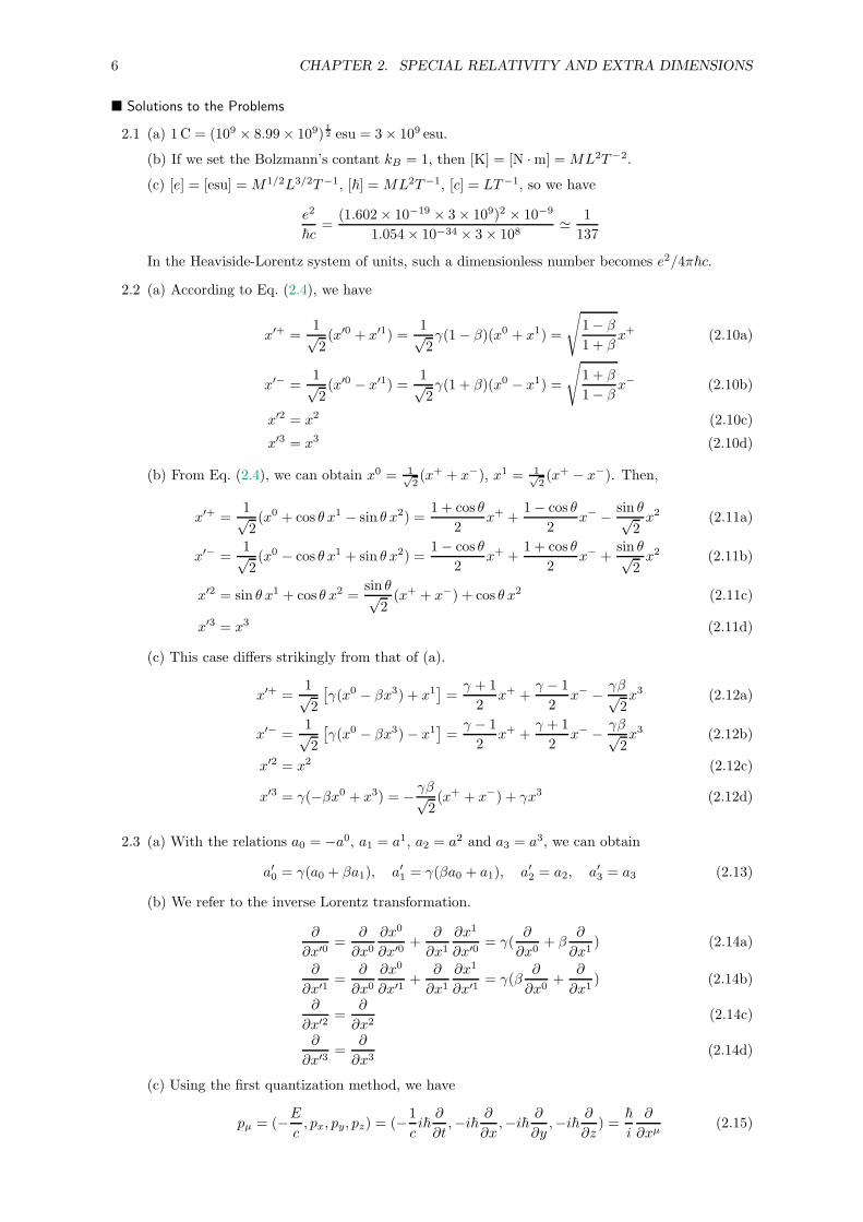
Solutions to the Problems

2.1 (a) 1C = (109 × 8.99× 109)12 esu = 3× 109 esu.

(b) If we set the Bolzmann’s contant kB = 1, then [K] = [N ·m] =ML2T−2.

(c) [e] = [esu] =M1/2L3/2T−1, [~] =ML2T−1, [c] = LT−1, so we have

e2

~c=

(1.602× 10−19 × 3× 109)2 × 10−9

1.054× 10−34 × 3× 108≃ 1

137

In the Heaviside-Lorentz system of units, such a dimensionless number becomes e2/4π~c.

2.2 (a) According to Eq. (2.4), we have

x′+ =1√2(x′0 + x′1) =

1√2γ(1− β)(x0 + x1) =

√

1− β

1 + βx+ (2.10a)

x′− =1√2(x′0 − x′1) =

1√2γ(1 + β)(x0 − x1) =

√

1 + β

1− βx− (2.10b)

x′2 = x2 (2.10c)

x′3 = x3 (2.10d)

(b) From Eq. (2.4), we can obtain x0 = 1√2(x+ + x−), x1 = 1√

2(x+ − x−). Then,

x′+ =1√2(x0 + cos θ x1 − sin θ x2) =

1 + cos θ

2x+ +

1− cos θ

2x− − sin θ√

2x2 (2.11a)

x′− =1√2(x0 − cos θ x1 + sin θ x2) =

1− cos θ

2x+ +

1 + cos θ

2x− +

sin θ√2x2 (2.11b)

x′2 = sin θ x1 + cos θ x2 =sin θ√

2(x+ + x−) + cos θ x2 (2.11c)

x′3 = x3 (2.11d)

(c) This case differs strikingly from that of (a).

x′+ =1√2

[

γ(x0 − βx3) + x1]

=γ + 1

2x+ +

γ − 1

2x− − γβ√

2x3 (2.12a)

x′− =1√2

[

γ(x0 − βx3)− x1]

=γ − 1

2x+ +

γ + 1

2x− − γβ√

2x3 (2.12b)

x′2 = x2 (2.12c)

x′3 = γ(−βx0 + x3) = − γβ√2(x+ + x−) + γx3 (2.12d)

2.3 (a) With the relations a0 = −a0, a1 = a1, a2 = a2 and a3 = a3, we can obtain

a′0 = γ(a0 + βa1), a′1 = γ(βa0 + a1), a′2 = a2, a′3 = a3 (2.13)

(b) We refer to the inverse Lorentz transformation.

∂

∂x′0=

∂

∂x0∂x0

∂x′0+

∂

∂x1∂x1

∂x′0= γ(

∂

∂x0+ β

∂

∂x1) (2.14a)

∂

∂x′1=

∂

∂x0∂x0

∂x′1+

∂

∂x1∂x1

∂x′1= γ(β

∂

∂x0+

∂

∂x1) (2.14b)

∂

∂x′2=

∂

∂x2(2.14c)

∂

∂x′3=

∂

∂x3(2.14d)

(c) Using the first quantization method, we have

pµ = (−Ec, px, py, pz) = (−1

ci~∂

∂t,−i~ ∂

∂x,−i~ ∂

∂y,−i~ ∂

∂z) =

~

i

∂

∂xµ(2.15)

7

2.4 (a) The identification yields a semi-circle. There are two fixed points: x = 0, 1. A foundamentaldomain can be chosen as [0, 1].

(b) As we know, x = ±1 are identified and y = ±1 are identified. Then it is obvious that thereare four fixed points: (0, 0), (0, 1), (1, 0) and (1, 1).

2.5 Let tan θ = β, then we can obtain the following from the inverse Lorentz transformation:

x0 = tan θ x1 + γ−1x′0, x0 = cot θ(x1 − γ−1x′1). (2.16)

It is obvious that the x′0 and x′1 axes appear in the original spacetime diagram as oblique axes.The angle between the x′0 axis and the x0 aixs is equal to that between the x′1 axis and the x1

axis, i.e. θ = arctanβ. Diagrams for the axes are drawn in Fig. 2.1.

θ

θ

x1

x0

x′1

x′0

Oθ

θ

θ

θ

x1

x0

x′1

x′0

O

Fig. 2.1 The left illustrates how the axes appear when β > 0, while the right is for β < 0.

2.6 (a) In light-cone coordinates, it can be written as (x+, x−) ∼ (x+, x− − 2√2πR).

(b) With the relations ct = γ(ct′ + βx′) and x = γ(βct′ + x′), we can obtain

(

βct′ + x′

ct′ + βx′

)

∼(

βct′ + x′

ct′ + βx′

)

+2π

γ

(

R−R

)

⇒(

x′

ct′

)

∼(

x′

ct′

)

+ 2π

√

1 + β

1− β

(

R−R

)

(2.17)

(c) From the following, we can see that the velocity parameter β = −R/√

R2 +R2s and that the

compactification radius Rc = Rs.

(

βct′ + x′

ct′ + βx′

)

∼(

βct′ + x′

ct′ + βx′

)

+2π

γ

(√

R2 +R2s

−R

)

⇒(

x′

ct′

)

∼(

x′

ct′

)

+ 2πγ

( √

R2 +R2s + βR

−R− β√

R2 +R2s

)

(d) For example, (0, 0) and (−2πR, 2π√

R2 +R2s) are related by the identification.

(e) Lightlike compactification with Radius R arises by boosting a standard compactification withradius Rs with Lorentz factor γ ∼

√

R2 +R2s/Rs, in the limits as Rs → 0.

2.7 (a) Using the result in 2.2 (a), we can rewrite the identification (x0, x1) ∼ (x′0, x′1) as

(x+, x−) ∼ (e−λx+, eλx−), where eλ =

√

1 + β

1− β(2.18)

The range of λ is (−∞,∞) and the orbifold fixed point is (0, 0).

(b) The spacetime diagram refers to Fig. 2.2. From Eq. (2.18), we see that e−λx+ ·eλx− = x+x−.So the idenfitication above relates points on the curves of x+x− = a2.

(c) −ds2 = −2dx+dx− = −2dx+d( a2

x+ ) = 2( ax+ )

2(dx+)2 > 0. Therefore, the interval is spacelike.

(d) We choose (eλ, e2λ) as the integrating interval, then we have

∫ e2λ

eλ

√2a

x−dx− =

√2aλ (2.19)

8 CHAPTER 2. SPECIAL RELATIVITY AND EXTRA DIMENSIONS

x1

x0x+x−

Fig. 2.2 The spacetime diagram for the x± axes and the family of curves x+x− = a2.

2.8 (a) The energy eigenvalues are Ekl =~2

2m

[

(kπa )2 + ( lR )2

]

, so we have

Z(a,R) =

∫ ∞

0

∫ ∞

0

exp(

− Ekl

kT

)

dk dl =mkTaR

2~2(2.20)

The results for a particle in a two-dimensional box with sides a and 2πR are the same.

(b) Since R≪ a, the lowest new energy level can be seen as E01. Then, we have

En0 < kT < E01 ⇒(nπ

a

)2

<2mkT

~2<

1

R2(2.21)

And Z(a,R) in this regime with the leading correction due to the small extra dimension is

Z(a,R) = exp(

− ~2

2mkTR2

)

∫ ∞

0

exp[

− ~2

2mkT

(kπ

a

)2]

dk =a√2mkT

~exp

(

− ~2

2mkTR2

)

Chapter 3

Electromagnetism and Gravitation

in Various Dimensions


1. Classical electrodynamics

• Maxwell’s equations in the Heaviside-Lorentz system of units

∇×E = −1

c

∂B

∂t(3.1a)

∇ ·B = 0 (3.1b)

∇ ·E = ρ (3.1c)

∇×B =1

cj +

1

c

∂E

∂t(3.1d)

• The Lorentz forcedp

dt= q

(

E +1

cv ×B

)

(3.2)

• Vector and scalar potentials

B = ∇×A (3.3a)

E = −1

c

∂A

∂t−∇Φ (3.3b)

2. Relativistic electrodynamics

Aµ = (Φ, A1, A2, A3), Aµ = (−Φ, A1, A2, A3) (3.4)

Fµν = ∂µAν − ∂νAµ =

0 −Ex −Ey −Ez

Ex 0 Bz −By

Ey −Bz 0 Bx

Ez By −Bx 0

(3.5)

∂λFµν + ∂µFνλ + ∂νFλµ = 0 (3.6)

jµ = (cρ, j1, j2, j3), ∂νFµν =

1

cjµ (3.7)

3. Gravitation and Planck’s length

− ds2 = gµν(x)dxµdxν , gµα(x)gαν (x) = δµν (3.8)

gµν(x) = ηµν + hµν(x), ∂2hµν − ∂α(∂µhνα + ∂νhµα) + ∂µ∂νh = 0 (3.9)

xµ′

= xµ + ǫµ(x), δhµν = ∂µǫν + ∂νǫµ (3.10)

ℓP =

√

~G

c3= 1.61× 10−33 cm, tP =

√

~G

c5= 5.4× 10−44 s, mP =

√

~c

G= 2.17× 10−5 g (3.11)

9

10 CHAPTER 3. ELECTROMAGNETISM AND GRAVITATION IN VARIOUS DIMENSIONS

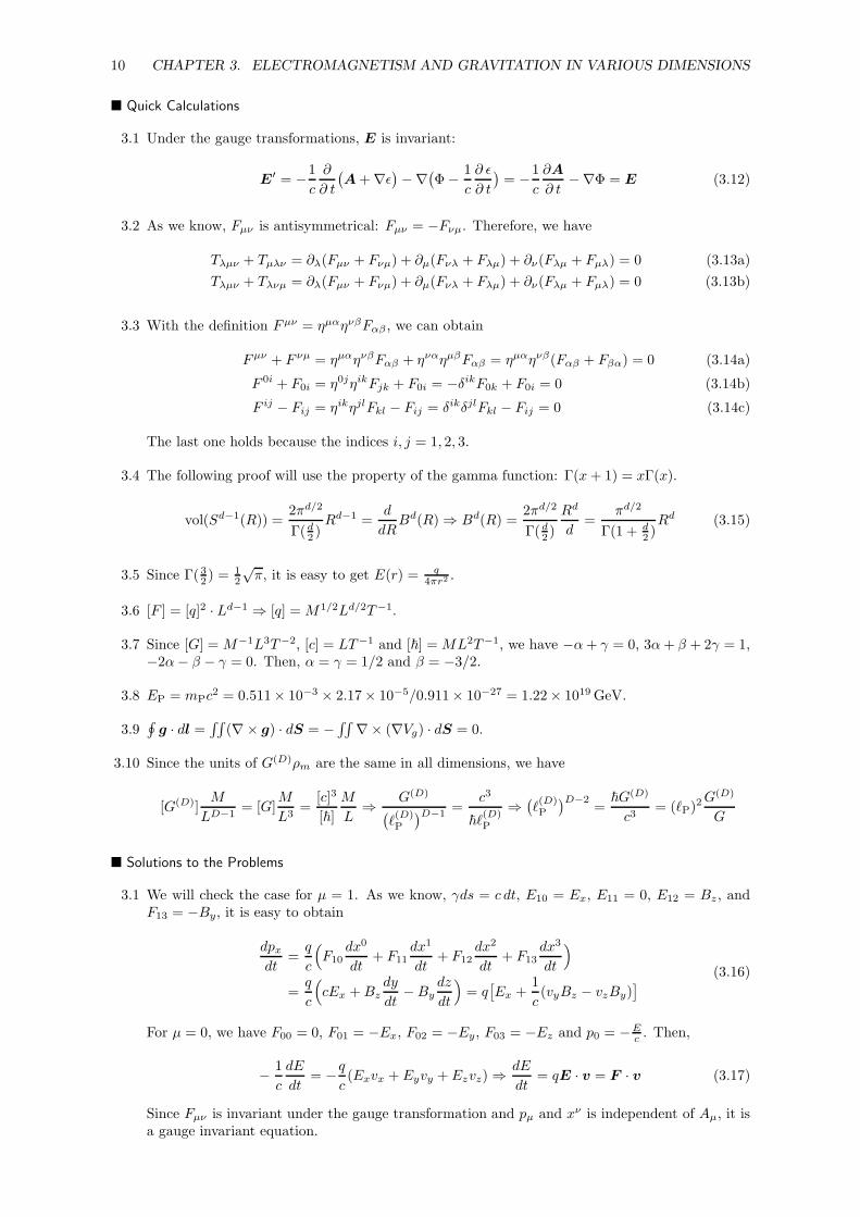
Quick Calculations

3.1 Under the gauge transformations, E is invariant:

E′ = −1

c

∂

∂ t

(

A+∇ǫ)

−∇(

Φ− 1

c

∂ ǫ

∂ t

)

= −1

c

∂A

∂ t−∇Φ = E (3.12)

3.2 As we know, Fµν is antisymmetrical: Fµν = −Fνµ. Therefore, we have

Tλµν + Tµλν = ∂λ(Fµν + Fνµ) + ∂µ(Fνλ + Fλµ) + ∂ν(Fλµ + Fµλ) = 0 (3.13a)

Tλµν + Tλνµ = ∂λ(Fµν + Fνµ) + ∂µ(Fνλ + Fλµ) + ∂ν(Fλµ + Fµλ) = 0 (3.13b)

3.3 With the definition Fµν = ηµαηνβFαβ , we can obtain

Fµν + F νµ = ηµαηνβFαβ + ηναηµβFαβ = ηµαηνβ(Fαβ + Fβα) = 0 (3.14a)

F 0i + F0i = η0jηikFjk + F0i = −δikF0k + F0i = 0 (3.14b)

F ij − Fij = ηikηjlFkl − Fij = δikδjlFkl − Fij = 0 (3.14c)

The last one holds because the indices i, j = 1, 2, 3.

3.4 The following proof will use the property of the gamma function: Γ(x+ 1) = xΓ(x).

vol(Sd−1(R)) =2πd/2

Γ(d2 )Rd−1 =

d

dRBd(R) ⇒ Bd(R) =

2πd/2

Γ(d2 )

Rd

d=

πd/2

Γ(1 + d2 )Rd (3.15)

3.5 Since Γ(32 ) =12

√π, it is easy to get E(r) = q

4πr2 .

3.6 [F ] = [q]2 · Ld−1 ⇒ [q] =M1/2Ld/2T−1.

3.7 Since [G] =M−1L3T−2, [c] = LT−1 and [~] =ML2T−1, we have −α+ γ = 0, 3α+ β + 2γ = 1,−2α− β − γ = 0. Then, α = γ = 1/2 and β = −3/2.

3.8 EP = mPc2 = 0.511× 10−3 × 2.17× 10−5/0.911× 10−27 = 1.22× 1019GeV.

3.9∮

g · dl =∫∫

(∇× g) · dS = −∫∫

∇× (∇Vg) · dS = 0.

3.10 Since the units of G(D)ρm are the same in all dimensions, we have

[G(D)]M

LD−1= [G]

M

L3=

[c]3

[~]

M

L⇒ G(D)

(

ℓ(D)P

)D−1=

c3

~ℓ(D)P

⇒(

ℓ(D)P

)D−2=

~G(D)

c3= (ℓP)

2G(D)

G


3.1 We will check the case for µ = 1. As we know, γds = c dt, E10 = Ex, E11 = 0, E12 = Bz, andF13 = −By, it is easy to obtain

dpxdt

=q

c

(

F10dx0

dt+ F11

dx1

dt+ F12

dx2

dt+ F13

dx3

dt

)

=q

c

(

cEx +Bzdy

dt−By

dz

dt

)

= q[

Ex +1

c(vyBz − vzBy)

]

(3.16)

For µ = 0, we have F00 = 0, F01 = −Ex, F02 = −Ey, F03 = −Ez and p0 = −Ec . Then,

− 1

c

dE

dt= −q

c(Exvx + Eyvy + Ezvz) ⇒

dE

dt= qE · v = F · v (3.17)

Since Fµν is invariant under the gauge transformation and pµ and xν is independent of Aµ, it isa gauge invariant equation.

11

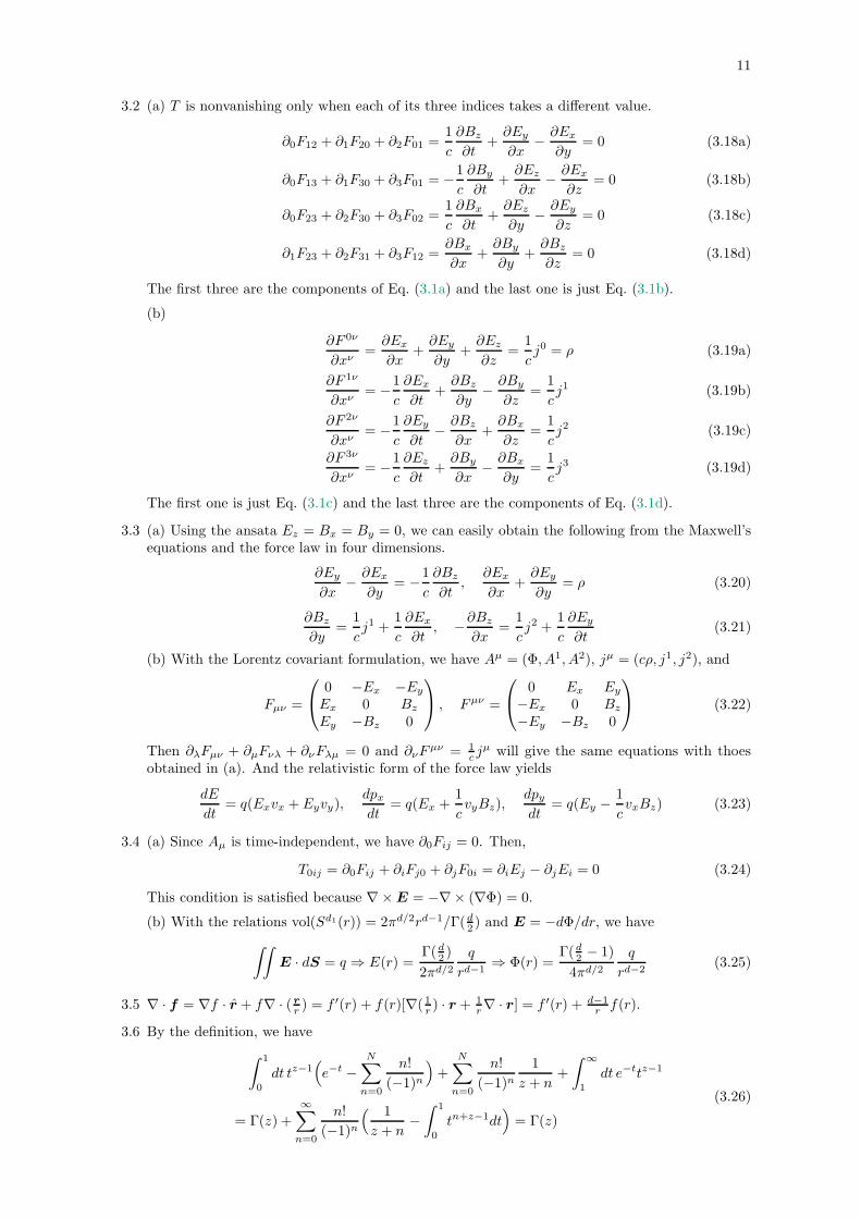
3.2 (a) T is nonvanishing only when each of its three indices takes a different value.

∂0F12 + ∂1F20 + ∂2F01 =1

c

∂Bz

∂t+∂Ey

∂x− ∂Ex

∂y= 0 (3.18a)

∂0F13 + ∂1F30 + ∂3F01 = −1

c

∂By

∂t+∂Ez

∂x− ∂Ex

∂z= 0 (3.18b)

∂0F23 + ∂2F30 + ∂3F02 =1

c

∂Bx

∂t+∂Ez

∂y− ∂Ey

∂z= 0 (3.18c)

∂1F23 + ∂2F31 + ∂3F12 =∂Bx

∂x+∂By

∂y+∂Bz

∂z= 0 (3.18d)

The first three are the components of Eq. (3.1a) and the last one is just Eq. (3.1b).

(b)

∂F 0ν

∂xν=∂Ex

∂x+∂Ey

∂y+∂Ez

∂z=

1

cj0 = ρ (3.19a)

∂F 1ν

∂xν= −1

c

∂Ex

∂t+∂Bz

∂y− ∂By

∂z=

1

cj1 (3.19b)

∂F 2ν

∂xν= −1

c

∂Ey

∂t− ∂Bz

∂x+∂Bx

∂z=

1

cj2 (3.19c)

∂F 3ν

∂xν= −1

c

∂Ez

∂t+∂By

∂x− ∂Bx

∂y=

1

cj3 (3.19d)

The first one is just Eq. (3.1c) and the last three are the components of Eq. (3.1d).

3.3 (a) Using the ansata Ez = Bx = By = 0, we can easily obtain the following from the Maxwell’sequations and the force law in four dimensions.

∂Ey

∂x− ∂Ex

∂y= −1

c

∂Bz

∂t,

∂Ex

∂x+∂Ey

∂y= ρ (3.20)

∂Bz

∂y=

1

cj1 +

1

c

∂Ex

∂t, −∂Bz

∂x=

1

cj2 +

1

c

∂Ey

∂t(3.21)

(b) With the Lorentz covariant formulation, we have Aµ = (Φ, A1, A2), jµ = (cρ, j1, j2), and

Fµν =

0 −Ex −Ey

Ex 0 Bz

Ey −Bz 0

, Fµν =

0 Ex Ey

−Ex 0 Bz

−Ey −Bz 0

(3.22)

Then ∂λFµν + ∂µFνλ + ∂νFλµ = 0 and ∂νFµν = 1

c jµ will give the same equations with thoes

obtained in (a). And the relativistic form of the force law yields

dE

dt= q(Exvx + Eyvy),

dpxdt

= q(Ex +1

cvyBz),

dpydt

= q(Ey −1

cvxBz) (3.23)

3.4 (a) Since Aµ is time-independent, we have ∂0Fij = 0. Then,

T0ij = ∂0Fij + ∂iFj0 + ∂jF0i = ∂iEj − ∂jEi = 0 (3.24)

This condition is satisfied because ∇×E = −∇× (∇Φ) = 0.

(b) With the relations vol(Sd1(r)) = 2πd/2rd−1/Γ(d2 ) and E = −dΦ/dr, we have

∫∫

E · dS = q ⇒ E(r) =Γ(d2 )

2πd/2

q

rd−1⇒ Φ(r) =

Γ(d2 − 1)

4πd/2

q

rd−2(3.25)

3.5 ∇ · f = ∇f · r + f∇ · (rr ) = f ′(r) + f(r)[∇(1r ) · r + 1r∇ · r] = f ′(r) + d−1

r f(r).

3.6 By the definition, we have

∫ 1

0

dt tz−1(

e−t −N∑

n=0

n!

(−1)n

)

+

N∑

n=0

n!

(−1)n1

z + n+

∫ ∞

1

dt e−ttz−1

= Γ(z) +

∞∑

n=0

n!

(−1)n

( 1

z + n−∫ 1

0

tn+z−1dt)

= Γ(z)

(3.26)


The function of the first integral has the order of O(tz+N ). For ℜ(z) > −N − 1, the integral on[0, 1] will always converge. So the right-hand side above is well defined. And also, we can obtainthe following identity:

Γ(z) =Γ(z +N + 1)

z(z + 1) · · · (z +N)(3.27)

Obviously, z = 0,−1,−2, . . ., are poles for Γ(z). The value of residue at z = −n is

Res[Γ(z),−n] = limz→−n

(z + n)Γ(z) =(−1)n

n!(3.28)

3.7 (a) The “gravitational” Bohr radius for a hydrogen atom is ~2/Gm3 = 2.2× 1032 m.

(b) Suppose kT = (8πM)−1Gαcβ~γ , then we have

[E] = [G]α[c]β [~]γM−1 ⇒ML2T−2 =M−α+γ−1L3α+β+2γT−2α−β−γ

⇒ α = −1, β = 3, γ = 1(3.29)

For M = 106M⊙, M⊙ = 2× 1030 kg, the temperature is T = 6.15× 10−14K. And for the blackhole whose temperature is room temperature (300K), its mass will be M = 4.2× 1020 kg.

3.8 We use the effective potential Veff(r) = Vg(r) + J2/2mr2 to discuss the planetary motion.

∫

Sd−1

g · dS =

∫

Bd

∇ · g d(vol) = −4πG(D)m⇒ g(r) = − 2Γ(d2 )

πd/2−1

G(D)m

rd−1= − d

drVg(r)

⇒ Vg(r) = −Γ(d2 − 1)

πd/2−1

G(D)m

rd−2

(3.30)

From the condition ddr

[

Veff(r)]∣

∣

r=r0= 0, we can solve r0. Then,

d2Veffdr2

∣

∣

∣

r=r0=

(4− d)J2

mr40(3.31)

For d = 3, it is positive, so the planetary circular orbits in the four-dimensional world are stableunder perturbations; while for d ≥ 4, they are not stable.

3.9 (a) Using the result in Eq. (3.30), we can directly write down the expression:

V (5)g (r) = −G

(5)M

πr2(3.32)

(b) The circel can be constructed by the identification of R1: w ∼ w + 2nπa, thus we have

V (5)g (x, y, z, 0) = −

∞∑

n=−∞

G(5)M

π[R2 + (2nπa)2](3.33)

(c) For R ≫ a, the potential becomes

V (5)g (x, y, z, 0) = −

∫ ∞

−∞

G(5)M

π

dt

R2 + (2πat)2= −G

(5)M

2πaR= −GM

R, (3.34)

in which we have used the relation G(5) = 2πaG.

3.10 (a) Using the following identity

∞∑

n=−∞

1

1 + (nπx)2=

1

xcoth

(1

x

)

, (3.35)

we can find an exact closed-form expression for the potential:

V (5)g (x, y, z, 0) = −G

(5)M

πR2

R

2acoth

( R

2a

)

= −GMR

coth( R

2a

)

(3.36)

13

(b) For R≫ a, we can expand the result above to the leading correction:

V (5)g (x, y, z, 0) = −GM

R

1 + e−λ

1− e−λ≃ −GM

R

(

1 + 2e−λ), (3.37)

where λ = R/a. When λ = 5.3, the correction is of order 1%.

(c) Using the following identity

cothx =1

x+x

3− x3

45+

2x5

945+ · · · , 0 < |x| < π, (3.38)

we can expand the gravitational potential when R ≪ a:

V (5)g (x, y, z, 0) ≃ −GM

R

(2a

R+R

6a

)

= −G(5)M

πR2

(

1 +R2

12a2

)

(3.39)

The first term has the same form to the gravitational potential discussed in 3.9 (a) .

Chapter 4

Nonrelativistic Strings


1. Equations of motion for transverse oscillations

∂2y

∂t2= v20

∂2y

∂x2, v0 =

√

T0µ0

(4.1)

y(t, x) = h+(x− v0t) + h−(x+ v0t) (4.2)

2. The nonrelativistic string Lagrangian

L(∂y

∂t,∂y

∂x

)

=1

2µ0

(∂y

∂t

)2

− 1

2T0

(∂y

∂x

)2

(4.3)

Pt =∂L∂y, Px =

∂L∂y′

,∂Pt

∂t+∂Px

∂x= 0 (4.4)

Quick Calculations

4.1 As we vary: y(t, x) → y(t, x) + δy(t, x), the variation is

δS = δ

∫ tf

ti

dt

∫ a

0

dx[1

2µ0

(∂y

∂t

)2

− 1

2T0

(∂y

∂x

)2]

=

∫ tf

ti

dt

∫ a

0

dx[

µ0∂y

∂t

∂(δy)

∂t− T0

∂y

∂x

∂(δy)

∂x

]

4.2 When we vary the motion by δy, the variation of the action is given by

δS =

∫ tf

ti

dt

∫ a

0

dx(

Ptδy + Pxδy′)

=

∫ tf

ti

dt

∫ a

0

dx[ ∂

∂t

(

Ptδy)

− ∂Pt

∂tδy +

∂

∂x

(

Pxδy)

− ∂Px

∂xδy

]

=

∫ a

0

(

Ptδy)∣

∣

∣

t=tf

t=tidx+

∫ tf

ti

(

Pxδy)∣

∣

∣

x=a

x=0dt−

∫ tf

ti

dt

∫ a

0

dx(∂Pt

∂t+∂Px

∂x

)

δy

(4.5)

4.3 With the relations Pt = µ0y and Px = −T0y′, we can rewrite Eq. (4.5) as

δS =

∫ a

0

(

Ptδy)∣

∣

∣

t=tf

t=tidx+

∫ tf

ti

(

Pxδy)∣

∣

∣

x=a

x=0dt−

∫ tf

ti

dt

∫ a

0

dx(∂Pt

∂t+∂Px

∂x

)

δy

=

∫ a

0

(

µ0∂y

∂tδy

)∣

∣

∣

t=tf

t=tidx+

∫ tf

ti

(

− T0∂y

∂xδy

)∣

∣

∣

x=a

x=0dt−

∫ tf

ti

dt

∫ a

0

dx(

µ0∂2y

∂t2− T0

∂2y

∂x2

)

δy


4.1 For small oscillations, the horizontal force dFh is

dFh = T0

[

1 +(∂y

∂x

)2]− 12

x+dx− T0

[

1 +(∂y

∂x

)2]− 12

x= −T0

∂y

∂x

∂2y

∂x2dx (4.6)

Since ∂y/∂x≪ 1, it is much smaller than the vertical force dFv.

15

16 CHAPTER 4. NONRELATIVISTIC STRINGS

4.2 For the small longitudinal oscillations, the equation can be derived as

T (x+ dx)− T (x) = τ0∂z

∂x

∣

∣

∣

x+dx− τ0

∂z

∂x

∣

∣

∣

x= τ0

∂2z

∂x2dx = µ0

∂2z

∂t2⇒ ∂2z

∂t2=τ0µ0

∂2z

∂x2(4.7)

Thus, the velocity of the waves is√

τ0/µ0.

4.3 (a) Suppose u = −v0t and w = u− a, then we can obtain the following:

y(t, 0) = h+(−v0t) + h−(v0t) = 0 ⇒ h+(u) = −h−(−u) (4.8)

y(t, a) = h+(a+u)+h−(a−u) = 0 ⇒ h+(u+ a)−h+(u− a) = 0 ⇒ h+(w) = h+(w+2a) (4.9)

(b) From the initial conditions, we have

y|t=0 = h+(x) + h−(x) = 0,∂y

∂t

∣

∣

∣

t=0= −v0h′+(x) + v0h

′−(x) (4.10)

The second equation can be rewritten by the integrating in two different intevals, which givesdifferent functions of h+(u). For 0 < x < a, we have

− h+(x) + h−(x) =

∫ x

0

ξ

a

(

1− ξ

a

)

dξ ⇒ h+(u) =1

2

( u3

3a2− u2

2a− c

)

(4.11)

For −a < x < 0, it becomes

− h+(x) + h−(x) =

∫ x

0

− ξa

(

1 +ξ

a

)

dξ ⇒ h+(u) =1

2

( u3

3a2+u2

2a+ c

)

(4.12)

We can extand h+(u) for all u with the periodic conditions h+(u) = h+(u+ 2a).

(c) For x and v0t in the domain D =

(x, v0t)| 0 ≤ x± v0t < a

, the wave function is

y(t, x) =1

2

[ (x− v0t)3

3a2− (x− v0t)

2

2a

]

− 1

2

[ (x+ v0t)3

3a2− (x+ v0t)

2

2a

]

= v0t(x

a− x2

a2− v20t

2

3a2

)

(4.13)

(d) From the function above, we can obtain

∂y

∂t= v0

(x

a− x2

a2− v20t

2

a2

)

= −v0[1

4−(x

a− 1

2

)2]

− v20t2

a2(4.14)

Obviously, at t = 0 the midpoint x = a/2 has the largest velocity. It is easy to concluce that thevelocity of the midpoint reaches zero at t0 = a/2v0 and y(t0, a/2) = a/12.

4.4

4.5

4.6 (a) The variation δS of the action under a variation δq of the coordinate can be derived as

δS = δ

∫

dt L(q(t), q(t); t) =

∫

dt(∂L

∂qδq +

∂L

∂qδq)

=

∫

dt[∂L

∂qδq +

d

dt

(∂L

∂qδq)

−( d

dt

∂L

∂q

)

δq]

=

∫

dt(∂L

∂q− d

dt

∂L

∂q

)

δq

(4.15)

Then, δS = 0 gives the famous Euler-Lagrange equation

∂L

∂q− d

dt

∂L

∂q= 0 (4.16)

(b) The derivation is similar to that in part (a):

δS = δ

∫

dDxL(φ(x), ∂µφ(x)) =∫

dDx[∂L∂φ

δφ+∂L∂∂µφ

δ(∂µφ)]

=

∫

dDx[∂L∂φ

δφ+ ∂µ

( ∂L∂∂µφ

δφ)

−(

∂µ∂L∂∂µφ

)

δφ]

=

∫

dDx(∂L∂φ

− ∂µ∂L∂∂µφ

)

δφ

(4.17)

Then we can obtain the Euler-Lagrange equation for the dynamical field φ(x)

∂L∂φ


= 0 (4.18)

Chapter 5

The Relativistic Point Particle


1. Action for a relativistic point particle

L = −mc2√

1− v2

c2, H =

mc2√

1− v2/c2, p =

∂L

∂v=

mv√

1− v2/c2(5.1)

xµ = xµ(τ), S = −mc∫

ds = −mc∫ τf

τi

√

−ηµνdxµ

dτ

dxν

dτdτ (5.2)

2. Equations of motion

δ(dxµ) = d(δxµ),dpµdτ

= 0,d2xµ

ds2= 0 (5.3)

S = −mc∫

Pds+

q

c

∫

PAµ(x) dx

µ (5.4)

Quick Calculations

5.1 Since xi and xf are fixed under the variation, we have

δSnr = δ

∫

1

2mv2 dt =

∫

mv · v0 dt = mv0 ·∫

dx = 0 (5.5)

5.2 For any arbitrary parameter τ ′(τ), we have

dpµdτ

=dpµdτ ′

dτ ′

dτ= 0 ⇒ dpµ

dτ ′= 0 (5.6)


5.1 For the new parameter τ = f(s), we have

d2xµ

ds2=

d

ds

(dxµ

dτ

df

ds

)

=d2xµ

dτ2

(df

ds

)2

+dxµ

dτ

d2f

ds2= 0 ⇒ d2f

ds2= 0 ⇒ f = as+ b, (5.7)

where a and b are constants independent of s.

5.2 If we reexpress the integrand ds using the parameterized world-line, i.e.

ds =

√

−ηµνdxµ

dτ

dxν

dτdτ (5.8)

then we can obtain the following

d2xλ

ds2=d2xλ

dτ2

(dτ

ds

)2

+dxλ

dτ

d2τ

ds2= 0 ⇒ ηµν

dxµ

dτ

dxν

dτ

d2xλ

dτ2− 1

2

dxλ

dτ

d

dτ

(

ηµνdxµ

dτ

dxν

dτ

)

= 0 (5.9)

5.3

17

18 CHAPTER 5. THE RELATIVISTIC POINT PARTICLE

5.4 (a) Using the relations Aµ = (−Φ,A) and dxµ/dt = (c,v), we can rewrite the action S as

S =

∫

1

2mv2 dt+

∫

q

c(−Φc+A · v) dt ⇒ L =

1

2mv2 − qΦ +

q

cA · v (5.10)

(b) By the definition, it is easy to get

p =∂L

∂v= mv +

q

cA · v (5.11)

(c) The Hamiltonian for the charged particle is given by

H = p ·v−L = mv2+q

cA ·v−

(mv2

2−qΦ+

q

cA ·v

)

=mv2

2+qΦ =

1

2m

(

p− q

cA)2

+qΦ (5.12)

5.5 The variation of the action for a charged point particle can be derived as

δS = −∫ τf

τi

dτ δxµdpµdτ

+q

c

∫ τf

τi

dτ[

δAµdxµ

dτ+Aµδ

(dxµ

dτ

)]

= −∫ τf

τi

dτ δxµdpµdτ

+q

c

∫ τf

τi

dτ[∂Aµ

∂xνδxν

dxµ

dτ+

d

dτ(Aµδx

µ)− dAµ

dτδxµ

]

= −∫ τf

τi

dτ δxµdpµdτ

+q

c

∫ τf

τi

dτ(∂Aµ

∂xνδxν

dxµ

dτ− ∂Aµ

∂xνdAν

dτδxµ

)

= −∫ τf

τi

dτ δxµdpµdτ

+q

c

∫ τf

τi

dτ(∂Aν

∂xµ− ∂Aµ

∂xν

)dxν

dτδxµ

=

∫ τf

τi

dτ(

− dpµdτ

+q

cFµν

dxν

dτ

)

δxµ

(5.13)

Then, δS = 0 gives the equation of motion:

dpµdτ

=q

cFµν

dxν

dτ(5.14)

5.6

5.7

Chapter 6

Relativistic Strings


1. Area functional for spatial surfaces

A =

∫

dξ1dξ2

√

( ∂x

∂ξ1· ∂x∂ξ1

)( ∂x

∂ξ2· ∂x∂ξ2

)

−( ∂x

∂ξ1· ∂x∂ξ2

)2

(6.1)

gij =∂x

∂ξi· ∂x∂ξi

, ds2 = gijdξidξj , A =

∫

dξ1dξ2√g, g = det(gij) (6.2)

2. The Nambu-Goto action

A =

∫

dτdσ

√

(∂X

∂τ· ∂X∂σ

)2

−(∂X

∂τ

)2(∂X

∂σ

)2

(6.3)

S = −T0c

∫ τf

τi

dτ

∫ σ1

0

dσ

√

(X ·X ′)2 − (X)2(X ′)2 (6.4)

γαβ = ηµν∂Xµ

∂ξα∂Xν

∂ξβ, S = −T0

c

∫

dτdσ√−γ, γ = det(γαβ) (6.5)

3. Equation of motion, boundary conditions, and D-branes

L(Xµ, Xµ′) = −T0c

√

(X ·X ′)2 − (X)2(X ′)2 (6.6)

Pτµ =

∂L∂Xµ

= −T0c

(X ·X ′)X ′µ − (X ′)2Xµ

√

(X ·X ′)2 − (X)2(X ′)2(6.7)

Pσµ =

∂L∂Xµ′ = −T0

c

(X ·X ′)Xµ − (X ′)2X ′µ

√

(X ·X ′)2 − (X)2(X ′)2(6.8)

Equation for relativistic string:∂Pτ

µ

∂τ+∂Pσ

µ

∂σ= 0 (6.9)

Dirichlet boundary condition:∂Xµ

∂τ(τ, σ∗) = 0, µ 6= 0, σ∗ = 0 or σ1 (6.10)

Free endpoint condition: Pσµ (τ, σ∗) = 0, σ∗ = 0 or σ1 (6.11)

4. Action in terms of transverse velocity

Xµ(τ, σ) = (ct,X(t, σ)),∂Xµ

∂τ= (c,

∂X

∂t),

∂Xµ

∂σ= (0,

∂X

∂σ) (6.12)

v⊥ =∂X

∂t−(∂X

∂t· ∂X∂s

)∂X

∂s, v2⊥ =

(∂X

∂t

)2

−(∂X

∂t· ∂X∂s

)2

(6.13)

S = −T0∫

dt

∫ σ1

0

dσ( ds

dσ

)

√

1− v2⊥c2, L = −T0

∫

ds

√

1− v2⊥c2

(6.14)

19

20 CHAPTER 6. RELATIVISTIC STRINGS

5. Motion of open string endpoints

Pσµ = −T0c2

(

1− v2⊥c2

)− 12(∂X

∂s· ∂X∂t

)

Xµ +[

c2 −(∂X

∂t

)2]∂Xµ

∂s

(6.15)

Pσ0 = −T0c

(

1− v2⊥c2

)− 12(∂X

∂s· ∂X∂t

)

= 0 ⇒ v · ∂X∂s

= 0 (6.16)

Pσµ = −T0(

1− v2

c2

)12 ∂Xµ

∂s= 0 ⇒ v2 = c2 (6.17)

Quick Calculations

6.1 Using the chain rule of derivatives, we can obtain

A =

∫

dξ1dξ2

√

( ∂x

∂ξ1· ∂x∂ξ1

)(∂ξ1

∂ξ1

)2( ∂x

∂ξ2· ∂x∂ξ2

)(∂ξ2

∂ξ2

)2

−( ∂x

∂ξ1· ∂x∂ξ2

)2(∂ξ1

∂ξ1∂ξ2

∂ξ2

)2

=

∫

dξ1dξ2

√

( ∂x

∂ξ1· ∂x∂ξ1

)( ∂x

∂ξ2· ∂x∂ξ2

)

−( ∂x

∂ξ1· ∂x∂ξ2

)2(6.18)

6.2 Using the chain rule, we can prove that

MijMjk =∂ξi

∂ξj∂ξj

∂ξk=∂ξi

∂ξk= δik, MijMjk =

∂ξi

∂ξj∂ξj

∂ξk=∂ξi

∂ξk= δik (6.19)

6.3 For a point on the world-sheet where all tangent vectors are spcelike with the exception of onethat is null, we have

∂X

∂τ=∂X

∂σ⇒ v2(λ) = (λ+ 1)2

∂X

∂σ≥ 0 (6.20)

When λ = −1, the tangent vector v = 0.

6.4 With the relations X · X ′ = XµX ′µ, (X)2 = XµXµ, and (X ′)2 = Xµ′X ′

µ, it is easy to verifyEq. (6.7) and Eq. (6.8).


6.1 Since the oscillations are small, we have

ds2 = dX · dX = (dx, dy) · (dx, dy) = dx2 + dy · dy ≃ dx2 (6.21)

Then the following approximation holds:

v⊥ =∂X

∂t−

(∂X

∂t· ∂X∂s

)∂X

∂s≃

(∂x

∂t,∂y

∂t

)

−(∂x

∂t,∂y

∂t

)

· (1, 0)(1, 0) =(

0,∂y

∂t

)

(6.22)

Furthermore, the action reduces to be

S ≃ −T0∫

dt

∫

dx

√

1− 1

c2

(∂y

∂t

)2

≃ −T0∫ tf

ti

dt

∫ a

0

dx[

1− 1

2c2

(∂y

∂t

)2]

(6.23)

Up to an additive constant−aT0(tf−ti), it is just the action for a nonrelativistic string performingsmall transverse oscillations, since µ0 = T0/c

2.

6.2 We start our derivation with the Nambu-Goto action and work in the static gauge:

S ≃ −T0c

∫ τf

τi

dτ

∫ σ1

0

dσ

√

0−(∂X

∂σ

)2

(−c2)

= −T0∫ tf

ti

dt

∫ 1

0

dσ∣

∣

∣

∂X

∂σ

∣

∣

∣

= −T0∫ tf

ti

dt

∫ a

0

dx

√

1 +(∂y

∂x

)2

≃ −T0∫ tf

ti

dt

∫ a

0

dx[

1 +1

2

(∂y

∂x

)2]

= −aT0(tf − ti)− T0

∫ tf

ti

dt

∫ a

0

dx1

2

(∂y

∂x

)2

(6.24)

21

6.3

6.4 In this problem, we are discussiong the time evolution of a closed circular string. It is clear tous that R(t) = v⊥, so we have

L = −T0∫

ds

√

1− R2(t)/c2 = −2πR(t)T0

√

1− R2(t)/c2 (6.25)

Then, we can obtain the Hamilonian

H = R∂L

∂R− L = − 2πT0RR

2√

1− R2/c2

(

− 2R

c2

)

+ 2πRT0

√

1− R2/c2 =2πR(t)T0

√

1− R2(t)/c2(6.26)

Acording to the energy onservation law, H = 0. It gives

d

dt

R(t)√

1− R2(t)/c2= 0 ⇒ R2(t)−R(t)R(t) = c2 ⇒ R(t) = R cos

(ct

R

)

, (6.27)

which has already satisfied the intial conditions: R(0) = R and R(0) = 0.

6.5 By the definition, it is easy to obtain

PσµPσµ =

T 20 [c

2 − (∂tX)2]

c2 − v2⊥

[

c2 − (∂tX)2]

(∂sX)2 − (∂sX · ∂tX)2

= 0 ⇒ v = |∂tX| = c (6.28)

6.6 From Eq. (6.14), we know that

L = −T0√

1− v2⊥c2

ds

dσ(6.29)

Then, the canonical momentum density and the Hamiltonian density are given by

P(t, σ) =∂L

∂(∂tX)= −T0

1

2

(

1− v2⊥c2

)− 12[

− 1

c2∂v2⊥

∂(∂tX)

] ds

dσ=T0c2

(

1− v2⊥c2

)− 12 ds

dσv⊥ (6.30)

H = P(t, σ) · ∂X∂t

− L =T0c2

(

1− v2⊥c2

)− 12 ds

dσv2⊥ + T0

√

1− v2⊥c2

ds

dσ=T0c2

(

1− v2⊥c2

)− 12 ds

dσ(6.31)

The total Hamiltonian can be written as

H =

∫

dσH =T0c2

∫

ds(

1− v2⊥c2

)− 12

= µ0

∫

ds(

1− v2⊥c2

)− 12

, (6.32)

where µ0 is the rest mass of a string rasing solely from the tension.

6.7 (a) The conditions satisfied by Pσ0 , Pσ

i , and Pσa at the endpoint are stated as follows:

Pσ0 (t, 0) = 0, Pσ

i (t, 0) = 0,∂Pσ

a

∂σ(t, 0) = 0 (6.33)

(b) If the string ends on a D0-brane, then the σ = 0 endpoint is fixed in the spacetime. Therefore,all boundary conditions are automatially satisfied.

(c) For a string ending on a D1-brane, we have

Pσ0 =

T0c

(

1− v2⊥c2

)− 12(∂X

∂s· ∂X∂t

)

= 0 ⇒ v · ∂X∂s

= 0 (6.34)

(d)

22 CHAPTER 6. RELATIVISTIC STRINGS

Chapter 7

String Parameterization and

Classical Motion


1. Choosing a σ parameterization

∂X

∂σ· ∂X∂t

= 0, v⊥ =∂X

∂t(7.1)

X ·X ′ = 0, X2 = −c2 + v2⊥, X ′2 =( ds

dσ

)2

(7.2)

Pτµ =T0c2

(

1− v2⊥c2

)− 12 ds

dσ

∂Xµ

∂t, Pσµ = −T0

(

1− v2⊥c2

)12 ∂Xµ

∂s(7.3)

∂

∂t

( T0√

1− v2⊥/c2

ds

dσ

)

= 0, H =

∫

T0ds√

1− v2⊥/c2

(7.4)

T0c2

1√

1− v2⊥/c2

∂v⊥∂t

=∂

∂s

(

T0

√

1− v2⊥c2∂X

∂s

)

, Teff = T0

√

1− v2⊥c2

(7.5)

2. Wave equation and constraints

dσ′ =ds

√

1− v2⊥/c2, σ1 ∈ [0, σ1], σ1 =

E

T0(7.6)

Wave equation:∂2X

∂σ2− 1

c2∂2X

∂t2= 0 (7.7)

Parameterization condition:∂X

∂t· ∂X∂σ

= 0 (7.8)

Parameterization condition:(∂X

∂σ

)2

+1

c2

(∂X

∂t

)2

= 1 (7.9)

Free boundary condition:∂X

∂σ

∣

∣

∣

σ=0=∂X

∂σ

∣

∣

∣

σ=σ1

= 0 (7.10)

Pτµ =T0c2∂Xµ

∂t, Pσµ = −T0

∂Xµ

∂σ(7.11)

3. General motion of an open string

X(t, σ) =1

2

[

F (ct+ σ) + F (ct− σ)]

, σ ∈ [0, σ1] (7.12)

∣

∣

∣

dF (u)

du

∣

∣

∣

2

= 1 and F (u + 2σ1) = F (u) +2σ1c

v0 (7.13)

F (u) =σ1π

(

cosπu

σ1, sin

πu

σ1

)

, X(t, σ) =σ1π

cosπσ

σ1

(

cosπct

σ1, sin

πct

σ1

)

(7.14)

23

24 CHAPTER 7. STRING PARAMETERIZATION AND CLASSICAL MOTION

Quick Calculations

7.1 With the periodic conditon of F (u), it is easy to show that

X(t = t0 + 2σ2/c, σ) =1

2

[

F (ct0 + 2σ1 + σ) + F (ct0 + 2σ1 − σ)]

=1

2

[

F (ct0 + σ) + F (ct0 − σ)]

+2σ1c

v0

= X(t = t0, σ) +2σ1c

v0

(7.15)

Therefore, v0 is the average velocity of any point σ on the string calculated over any time intervalof duration 2σ1/c.


7.1 (d) The length ℓ of an open string parameterized with engery is given by

ds =

√

1− v2⊥c2

dσ ⇒ ℓ =

∫ σ1

0

√

1− v2⊥c2

dσ (7.16)

7.2 (a) For the rotating string, we have v⊥ = ωs = 2cs/ℓ. Then, the following holds

E(s) = dE

ds=

T0√

1− v2⊥/c2=

T0√

1− 4s2/ℓ2(7.17)

It has singularities at the endpoints s = ±ℓ/2. And the total energy is given by

E =

∫

ds E(s) =∫ ℓ/2

−ℓ/2

dsT0

√

1− 4s2/ℓ2=π

2ℓT0 (7.18)

(b) The average energy density is πT0/2, so we have

T0√

1− 4s2/ℓ2=π

2T0 ⇒ s = ±

√π2 − 4

2πℓ (7.19)

(c) The energy carried by the string on the interval [−s, s] is given by

E =

∫ s

−s

dxT0

√

1− 4x2/ℓ2= ℓT0 arcsin

2s

ℓ(7.20)

7.3 (a) The general solution for X(t, σ) in terms of a vector function F (u) is given by

X(t, σ) =1

2

[

F (ct+ σ) + F (ct− σ)]

(7.21)

The following parameterization conditions are required

(∂X

∂σ± 1

c

∂X

∂t

)2

= 1 ⇒∣

∣

∣

dF (u)

du

∣

∣

∣

2

= 1 (7.22)

∂X

∂t(0, σ) =

c

2

[

F ′(σ) + F ′(−σ)]

= 0 ⇒ dF (−u)du

= −dF (u)

du⇒ F (u) = F (−u) (7.23)

(b) We should impose this condition: X(t, σ + σ1) = X(t, σ), i.e.

F (ct + σ + σ1) + F (ct− σ − σ1) = F (ct+ σ) + F (ct− σ)

⇒ F (σ + σ1) + F (−σ − σ1) = F (σ) + F (−σ)⇒ F (σ + σ1) = F (σ)

(7.24)

(c) tP = σ1/c, X(tP, σ) = X(0, σ).

25

7.4 (a) Using the boundary condition at σ = σ1, we find

X(t, σ1) = x1 +1

2

[

F (ct + σ1)− F (ct− σ1)]

= x2 ⇒ F (u+ 2σ1)− F (u) = 2(x2 − x1) (7.25)

(b) From the parameterization conditions, we can obtain

(∂X

∂σ± 1

c

∂X

∂t

)2

= 1 ⇒∣

∣

∣

dF (u)

du

∣

∣

∣

2

= 1 (7.26)

(c) According to the information above, we have

∂X

∂σ(t, 0) = F ′(ct) = (sin γ cosωt, sin γ sinωt, cos γ)

⇒ F ′(u) =(

sin γ cosuω

c, sin γ sin

uω

c, cos γ

)

⇒ F (u) =( c

ωsin γ sin

uω

c,− c

ωsin γ cos

uω

c, u cosγ

)

(7.27)

(d) Using the result in part (a), it is easy to obtain

2( c

ωsin γ cos

(u + σ1)ω

csin

σ1ω

c,c

ωsin γ sin

(u + σ1)ω

csin

σ1ω

c, σ1 cos γ

)

=2(x2 − x1) = 2(0, 0, L0) ⇒ ω =cπ

σ1, σ1 =

L0

cos γ

(7.28)

(e) Now, we can directly write down the wave function for this relativistic jumping rope:

X(t, σ) =(σ1π

sin γ cosπct

σ1sin

πσ

σ1,σ1π

sin γ sinπct

σ1sin

πσ

σ1, σ cos γ

)

(7.29)

(f) First, we calculate the value of v2⊥:

v⊥ =(

− c sin γ sinπct

σ1sin

πσ

σ1, c sin γ cos

πct

σ1sin

πσ

σ1, 0)

⇒ v2⊥ = c2 sin2 γ sin2(πσ

σ1

)

(7.30)

Then, the energy distributed in the string is given by

E(z) = T0

(

1− v2⊥c2

)− 12

= T0

[

1− sin2 γ sin2(πσ

σ1

)]− 12

= T0

[

1− sin2 γ sin2(πz

L0

)]− 12

(7.31)

7.5 (a) This ansatz is consistent with the constraints on F (u).

(b) It is easy to see that X ′(t, σ) = 12

[

F ′(ct+ σ) + F ′(ct− σ)]

, so we have

X ′(0, 0) = F ′(σ) ⇒ dy

dσ= sin

(

γ cosπσ

σ1

)

(7.32)

(c) X ′(t, 0) = F ′(ct).

(d) We will find an integral relation between a, σ1 and γ:

F (u + 2σ)− F (u) =(

∫ u+2σ1

u

cos[

γ cosπx

σ1

]

dx,

∫ u+2σ1

u

sin[

γ cosπx

σ1

]

dx)

=(

∫ 2σ1

0

cos[

γ cosπx

σ1

]

dx,

∫ 2σ1

0

sin[

γ cosπx

σ1

]

dx)

=(

∫ 2σ1

0

cos[

γ cosπx

σ1

]

dx, 0)

⇒ a =

∫ σ1

0

cos(

γ cosπx

σ1

)

dx

(7.33)

Assume that γ is small, then the following approxiamtion holds:

a ≃∫ σ1

0

(

1− 1

2γ2 cos2

πx

σ1

)

dx = σ1

(

1− 1

4γ2

)

(7.34)

(e) Using the following identity

J0(z) =1

π

∫ π

0

cos(z cos θ) dθ, (7.35)

we can obtain

a =

∫ σ1

0

cos(

γ cosπx

σ1

)

dx =σ1π

∫ π

0

cos(γ cos θ) dθ ⇒ a

σ1= J0(γ) (7.36)

26 CHAPTER 7. STRING PARAMETERIZATION AND CLASSICAL MOTION

7.6 (a) We only need to examine the components.

1

2

cos[

γ cosπ(ct+ σ)

σ1

]

+ cos[

γ cosπ(ct− σ)

σ1

]

=cosγ

2

[

cosπ(ct+ σ)

σ1+ cos

π(ct− σ)

σ1

]

cosγ

2

[

cosπ(ct+ σ)

σ1− cos

π(ct− σ)

σ1

]

=cos(

γ cosπct

σ1cos

πσ

σ1

)

cos(

γ sinπct

σ1sin

πσ

σ1

)

(7.37)

1

2

sin[

γ cosπ(ct+ σ)

σ1

]

+ sin[

γ cosπ(ct− σ)

σ1

]

=sinγ

2

[

cosπ(ct+ σ)

σ1+ cos

π(ct− σ)

σ1

]

cosγ

2

[

cosπ(ct+ σ)

σ1− cos

π(ct− σ)

σ1

]

=sin(

γ cosπct

σ1cos

πσ

σ1

)

cos(

γ sinπct

σ1sin

πσ

σ1

)

(7.38)

When ct = σ1/2, the second component is zero. That is to say, the string is horizontal.

(b) It is easy to see that X/c = 12

[

F ′(ct+ σ)− F ′(ct− σ)]

. Then we have

1

2

cos[

γ cosπ(ct+ σ)

σ1

]

− cos[

γ cosπ(ct− σ)

σ1

]

=− sinγ

2

[

cosπ(ct+ σ)

σ1+ cos

π(ct− σ)

σ1

]

sinγ

2

[

cosπ(ct+ σ)

σ1− cos

π(ct− σ)

σ1

]

=− sin(

γ cosπct

σ1cos

πσ

σ1

)

sin(

γ sinπct

σ1sin

πσ

σ1

)

(7.39)

1

2

sin[

γ cosπ(ct+ σ)

σ1

]

− sin[

γ cosπ(ct− σ)

σ1

]

=cosγ

2

[

cosπ(ct+ σ)

σ1+ cos

π(ct− σ)

σ1

]

sinγ

2

[

cosπ(ct+ σ)

σ1− cos

π(ct− σ)

σ1

]

=cos(

γ cosπct

σ1cos

πσ

σ1

)

sin(

γ sinπct

σ1sin

πσ

σ1

)

(7.40)

Therefore, the instantaneous transverse velocity satisfies

∣

∣

∣

1

c

∂X

∂t

∣

∣

∣ =∣

∣

∣ sin(

γ sinπct

σ1sin

πσ

σ1

)∣

∣

∣ (7.41)

For γ = π/2, the string midpoint σ = σ1/2 reaches the speed of lignt when ct = σ1/2, meaningthat the string is horizontal.

(c) For γ =√2π/2 and ct = σ1/4, we have

∣

∣

∣sin

( π√2

1√2sin

πσ

σ1

)∣

∣

∣= 1 ⇒ σ =

σ12

(7.42)

For ct = σ1/3, we have

∣

∣

∣ sin( π√

2

√3

2sin

πσ

σ1

)∣

∣

∣ = 1 ⇒ σ = 0.174σ1 or 0.826σ1 (7.43)

Chapter 8

World-sheet Currents


1. Conserved currents on the world-sheet

S =

∫

dξ0dξ1L(∂0Xµ, ∂1Xµ), (ξ0, ξ1) = (τ, σ) (8.1)

jαµ =∂L

∂(∂αXµ), (j0µ, j

1µ) =

( ∂L∂Xµ

,∂L∂Xµ′

)

= (Pτµ ,Pσ

µ ) (8.2)

pµ(τ) =

∫ σ1

0

Pτµ dσ,

dpµdτ

= 0, pµ =

∫

γ

(Pτµdσ − Pσ

µdτ) (8.3)

2. Lorentz symmetry and associated currents

Xµ → Xµ + δXµ, δXµ = ǫµνXν , ǫµν = −ǫνµ (8.4)

Mαµν = XµPα

ν −XνPαµ ,

∂Mτµν

∂τ+∂Mσ

µν

∂σ= 0 (8.5)

Mµν =

∫

γ

(Mτµν dσ −Mσ

µν dτ), Mµν = −Mνµ (8.6)

3. The slope parameter α′

J

~= α′E2, J =

E2

2πT0c, α′ =

1

2πT0~c(8.7)

Quick Calculations

8.1 We will use the divergence theorem to prove the result.

dQi

dξ0=

∫

dξ1dξ2 · · · dξk ∂j0i

∂ξ0= −

∫

dξ1dξ2 · · · dξk(∂j1i∂ξ1

+∂j2i∂ξ2

+ · · ·+ ∂jki∂ξk

)

= −∫

∂V

j · dA = 0

8.2 For the fixed 2-by-2 matrix Aab that satisfies Aabvavb = 0, we have

A11v1v1 +A12v1v2 +A21v2v1 +A22v2v2 = 0 ⇒ A11 = 0, A12 = −A21, A22 = 0 (8.8)

8.3 For a 4-by-4 matrix ǫµν that satisfies ǫµνvµvν = 0, the conclusion is the same: ǫµν must beantisymmetric.

8.4 ǫµν = ηµαηνβǫαβ = −ηµαηνβǫβα = −ηαµηβνǫβα = −ǫνµ.

8.5 For the boost with very small β, we have

x′0 − x0 = (γ − 1)x0 − γβx1 ≃ −βx1 ⇒ ǫ01 = −β (8.9)

x′1 − x1 = −γβx0 + (γ − 1)x1 ≃ βx0 ⇒ ǫ10 = β (8.10)

And all other values are zero.

27

28 CHAPTER 8. WORLD-SHEET CURRENTS

8.5 J = Iω, E = 12Iω

2 ⇒ J ∼√E.

8.6 [α′] = [E]−2, [~] = [E]T , [c] = LT−1 ⇒ [ℓs] = L.


8.1 (a) The variation can be written as δq(t) = ǫn× q, where ǫ is an infinitesimal constant and n isthe rotation axis. Then we have

q′ = q + ǫn× q ⇒ q′2 = q2 + ǫ2(n× q)2 ≃ q2 (8.11)

The Lagrangian only depends on q2, therefore L is invariant.

(b) The conserved charge associated with this symmetry transformation is given by

ǫQ =∂L

∂q· δq = p · (n× q) = n · (q × p) = n · J , (8.12)

where J is the vector angular momentum.

8.2 (a) The variation of coordinates and the conserved charges are given by

δqi(t) = ǫi(t)h(q(t); t), ǫiQi =∂L

∂qaδqa (8.13)

Considering the Euler-Lagrange equations, we can obtain

ǫidQi

dt=

d

dt

( ∂L

∂qa

)

δqa +∂L

∂qad

dt(δqa) =

∂L

∂qaδqa +

∂L

∂qad

dt(δq) = 0 (8.14)

(b) For a world with no spatial dimentions, α = 0. And the corresponding equations become

ǫij0i =∂L∂φa

δφa,d

dtj0i = 0, Qi = cqi (8.15)

8.3

8.4 (a) T0 = 8.5× 1014GeV ·m−1, ℓs = 1.92× 10−14 cm.

(b) α′ = 2.58× 10−33GeV−2, T0 = 3× 1047GeV ·m−1.

8.5 For the relativistic jumping rope, we have

X(t, σ) =(σ1π

sin γ cosπct

σ1sin

πσ

σ1,σ1π

sin γ sinπct

σ1sin

πσ

σ1, σ cos γ

)

(8.16)

Pτ =

T0c2∂X

∂t=T0c

sin γ sinπσ

σ1

(

− sinπct

σ1, cos

πct

σ1, 0)

(8.17)

Then, the z-component of angular momentum is given by

Jz =M12 =

∫ σ1

0

(X1Pτ2 −X2Pτ

1 ) dσ =T0σ1πc

sin2 γ

∫ σ1

0

sin2πσ

σ1dσ =

T0σ21

2πcsin2 γ (8.18)

Since σ1 = E/T0, we have found

Jz =E2

2πT0csin2 γ ⇒ Jz

~= (sin2 γ)α′E2 (8.19)

8.6 With the Euler-Lagrange equation, we can show that

ǫdQ

dt=

d

dt

(∂L

∂q

)

δq +∂L

∂q

d

dt(δq)− ǫ

dΛ

dt=∂L

∂qδq +

∂L

∂qδq − δL = 0 (8.20)

For the transformation q(t) → q(t) + ǫq(t), we have

δL =∂L

∂qδq +

∂L

∂qδq = ǫ

[ d

dt

(∂L

∂q

)

q +∂L

∂qq]

= ǫd

dt

(∂L

∂qq)

⇒ Λ =∂L

∂qq (8.21)

ǫQ =∂L

∂qδq − ǫΛ =

∂L

∂qq − ǫΛ ⇒ Q = 0 (8.22)

29

8.7 The proof is very similar to that in Eq. (8.20):

ǫi∂jαi∂ξα

=∂

∂ξα

[ ∂L∂(∂αφa)

]

δφa +∂L

∂(∂αφa)

∂δφa

∂ξα− ǫi

∂Λαi

∂ξα

=∂L∂φa

δφa +∂L

∂(∂αφa)δ(∂αφ

a)− δL = 0

(8.23)

For the transformation φa(ξβ) → φa(ξβ) + ǫβ∂βφa, we have

δL =∂L∂φa

δφa +∂L

∂∂αφaδ(∂αφ

a) = ǫβ[ ∂

∂ξα

( ∂L∂∂αφa

)

∂βφa +

∂L∂∂αφa

∂α∂βφa]

= ǫβ∂

∂ξα

( ∂L∂∂αφa

∂βφa)

⇒ Λαβ =

∂L∂∂αφa

∂βφa = δαβL

(8.24)

ǫβjαβ =∂L

∂∂αφaδφa − ǫβΛα

β = ǫβ( ∂L∂∂αφa

∂βφa − δαβL

)

⇒ jαβ =∂L

∂∂αφa∂βφ

a − δαβL (8.25)

It is easy to see that j00 = H, i.e. the Hamiltonian density.

30 CHAPTER 8. WORLD-SHEET CURRENTS

Chapter 9

Light-cone Relativistic Strings


1. The σ parameterizationX0(τ, σ) = cτ, nµX

µ(τ, σ) = λτ (9.1)

~ = c = 1, L = T, M = L−1, ℓs =√α′ (9.2)

S = − 1

2πα′

∫ τf

τi

dτ

∫ σ1

0

dσ

√

(X ·X ′)2 − (X)2(X ′)2 (9.3)

open strings: (n · p)σ = π

∫ σ

0

dσ n · Pτ (τ, σ), n ·X(τ, σ) = 2α′(n · p)τ (9.4)

closed strings: (n · p)σ = 2π

∫ σ

0

dσ n · Pτ (τ, σ), n ·X(τ, σ) = α′(n · p)τ (9.5)

2. Constraints and wave equations

X ·X ′ = 0, X2 +X ′2 = 0, (X ±X ′)2 = 0 (9.6)

Pτµ =1

2πα′ Xµ, Pσµ = − 1

2πα′Xµ′, Xµ −Xµ′′ = 0 (9.7)

3. Wave equation and mode expansions

Xµ(τ, σ) = fµ0 + fµ

1 τ +∞∑

n=1

(Aµn cosnτ + Bµ

n sinnτ) cosnσ (9.8)

Aµn cosnτ +Bµ

n sinnτ = −i√

2α′/n (aµ∗n einτ − aµne−inτ ), fµ

1 = 2α′pµ (9.9)

Xµ(τ, σ) = xµ0 + 2α′pµτ − i√2α′

∞∑

n=1

(aµ∗n einτ − aµne−inτ )

cosnσ√n

(9.10)

αµ0 =

√2α′pµ, αµ

n = aµn√n, αµ

−n = aµ∗n√n, n ≥ 1 (9.11)

Xµ(τ, σ) = xµ0 +√2α′αµ

0 τ + i√2α′

∑

n6=0

1

nαµne

−inτ cosnσ (9.12)

Xµ ±Xµ′ =√2α′

∑

n∈Z

αµne

−in(τ±σ) (9.13)

4. Light-cone solution of equations of motion

nµ =( 1√

2,1√2, 0, . . . , 0

)

, n ·X = X+, n · p = p+ (9.14)

X+(τ, σ) = βα′p+τ, p+σ =2π

β

∫ σ

0

dσ pτ+(τ, σ), β = 2, 1 (9.15)

XI = (X2, X3, . . . , Xd), X− ±X−′ = (2βα′p+)−1(XI ±XI′)2 (9.16)

31

32 CHAPTER 9. LIGHT-CONE RELATIVISTIC STRINGS

x+0 = 0, α+n = α+

−n = 0, n = 1, 2, . . . ,∞ (9.17)

√2α′α−

n =1

p+L⊥n , L⊥

n =1

2

∑

p∈Z

αIn−pα

Ip, 2p+p− =

1

α′L⊥0 (9.18)

X− ±X−′ =1

p+

∑

n∈Z

L⊥n e

−in(τ±σ) =1

4α′p+(X− ±X−′)2 (9.19)

M2 = 2p+p− − pIpI =1

α′

∞∑

n=1

naI∗n aIn (9.20)

Quick Calculations

9.1 e = ~c/ℓ = 2× 10−5 × 1018 = 2× 1013 eV = 20TeV.

9.2 Since tµtµ < 0, then we can prove the vector vµ is timelike:

vµvµ =(

tµ − t ·X ′

X ′ ·X ′Xµ′)(

tµ − t ·X ′

X ′ ·X ′X′µ

)

= tµtµ − (t ·X ′)2

X ′ ·X ′ < 0 (9.21)

9.3 It is obvious that Xµ(τ, σ) is real.

9.4 Using the relation√2α′α−

0 = L⊥n /p

+, we can rewrite the expression as

X−(τ, σ) = x−0 +√2α′α−

0 τ + i√2α′

∑

n6=0

1

nα−n e

−inτ cosnσ

= x−0 +1

p+L⊥0 τ +

i

p+

∑

n6=0

1

nL⊥n e

−inτ cosnσ

(9.22)

9.5 When all aIn vanish, we have L⊥n = 0 for n ≥ 1. Therefore, X−(τ, σ) = x−0 +

√2α′α−

0 τ .


9.1 (a) (nµ + bµ)(nµ + bµ) = bµb

µ ≥ 0. Therefore, bµ is spacelike of null.

(b) If bµ is null, we have bµ(nµ−λbµ) = 0 and λnµ)(n

µ−λbµ) = 0. Then (bµ−λnµ)(nµ−λbµ) = 0.

Therefore, bµ = λnµ.

(c) The set of vectors bµ that satisfies nµbµ = 0 is a hyperplane orthogonal to the vector nµ.

Therefore, it is a space of dimension (D1). And the subset of null vectors forms a subspace ofdimension one.

(d) For D = 2 and n ·X = X+, we can obtain

nµ =( 1√

2,1√2

)

, nµ =(

− 1√2,1√2

)

(9.23)

9.2 (a) Using Eq. (9.16), we can find

∂τX− =

(∂τXI)2 + (∂σX

I)2

2βα′p+, ∂σX

− =(∂τX

I)(∂σXI)

βα′p+(9.24)

From the consistency condtion ∂σ∂τX− = ∂τ∂σX

−, it is easy to prove that

∂σ[

(∂τXI)2 + (∂σX

I)2]

= 2∂τ[

(∂τXI)(∂σX

I)]

⇒ ∂2τXI = ∂2σX

I (9.25)

(b) If the transverse coordinates XI satisfy the wave function, then it follows

∂2τX− − ∂2σX

− = (βα′p+)−1(∂2τXI)(∂2τX

I − ∂2σXI) = 0 (9.26)

(c) The coordinates satisfying Neumann boundary conditions means that ∂σXI = 0 at σ = 0, π,

while satisfing Dirichlet boundary conditions indicates that ∂τXI = 0. Since ∂σX

− is determinedby the product of ∂τX

I and ∂σXI , it is always zero. Therefore, X− will always satisfy Neumann

boundary conditions.

33

9.3 (a) M2 = (α′)−1∑∞

n=1 αµnα

µ−n = (α′)−1(a2 + a2) = 2a2/α′.

(b) The length of the string is given by l = 2πMα′ = 2πa√2α′. And the explicit functions of

X(2)(τ, σ) and X(3)(τ, σ) are given by

X(2)(τ, σ) = x(2)0 + i

√2α′a(e−iτ − eiτ ) cosσ = 2

√2α′a sin τ cosσ (9.27)

X(3)(τ, σ) = x(3)0 + i

√2α′ia(e−iτ + eiτ ) cosσ = −2

√2α′a cos τ cosσ (9.28)

(c) L⊥0 = 1

2

[

α(2)−1α

(2)1 + α

(3)−1α

(3)1

]

= a2, L⊥0 = 0 (n 6= 0). X−(τ, σ) = a2τ/p+.

(d) τ = ωt = πt/l. The value of p+ can be determined by the following

X1(τ, σ) =1√2(X+ −X−) = (

√2p+α′ − a2√

2p+)τ = 0 ⇒ p+ =

a√2α′

(9.29)

9.4 (a)

X2(τ, σ) = x20 + i√2α′a(e−iτ − eiτ ) cosσ = 2

√2α′a sin τ cosσ (9.30)

34 CHAPTER 9. LIGHT-CONE RELATIVISTIC STRINGS

Chapter 10

Light-cone Fields and Particles


1. Classical scalar fields

S =

∫

dDx(

− 1

2ηµν∂µφ∂νφ− 1

2m2φ2

)

, (∂2 −m2)φ = 0 (10.1)

φ(t,x) = ae−iEpt+ip·x + a∗eiEpt−ip·x, Ep =√

p2 +m2 (10.2)

φ(x) =

∫

dDp

(2π)Deip·xφ(p), (p2 −m2)φ(p) = 0 (10.3)

xT = (x2, x3, . . . , xd),(

− 2∂

∂x+∂

∂x−+

∂

∂xI∂

∂xI−m2

)

φ(x+, x−,xT ) = 0 (10.4)

pT = (p2, p3, . . . , pd),[

i∂

∂x+− 1

2p+(

pIpI +m2)

]

φ(x+, p+,pT ) = 0 (10.5)

x+ =p+τ

m2,

[

i∂

∂τ− 1

2m2

(

pIpI +m2)

]

φ(τ, p+,pT ) = 0 (10.6)

[

ap, a†p

]

= 1,[

a−p, a†−p

]

= 1,[

a(t), a†(t)]

=[

a†(t), a(t)]

= 2iEp (10.7)

H = Ep

(

a†pap + a†−pa−p

)

, P = p(

a†pap − a†−pa−p

)

(10.8)

2. Maxwell fields∂2Aµ − ∂µ(∂ · A) = 0, p2Aµ − pµ(p · A) = 0 (10.9)

Aµ(p) → Aµ(p) + ipµǫ(p), A+(p) = 0 (10.10)

p · A = 0, p+A− = pIAI , p2AI = 0 (10.11)

3. Gravitational fieldsp2hµν − pα(p

µhνα + pνhµα + pµpνh = 0 (10.12)

δhµν(p) = ipµǫν(p) + ipνǫµ(p), δh = 2ip · ǫ (10.13)

h++ = h+− = h+I = 0, h = 0, hII = 0, p2hµν = 0 (10.14)

p+hI− = pJhIJ , p+h−− = pIh

−I , p2hIJ = 0 (10.15)

Quick Calculations

10.1 By the definition, we have

H = Π∂0φ− L = Π2 −[1

2Π2 − 1

2(∇φ)2 − 1

2m2φ2

]

=1

2Π2 +

1

2(∇φ)2 + 1

2m2φ2 (10.16)

10.2 With the mass-shell condition, we have

p2 +m2 = −2p+p− + pIpI +m2 = 0 ⇒ p− =1

2p+(

pIpI +m2)

(10.17)

35

36 CHAPTER 10. LIGHT-CONE FIELDS AND PARTICLES

10.3 ∂0φp and ∇φp are given by

∂0φp =1

√

2V Ep

[

a(t)eip·x + a∗(t)e−ip·x], ∇φp =i

√

2V Ep

[

a(t)eip·x − a∗(t)e−ip·x]p (10.18)

Using the quantization condition, we can integrate the action as

S =

∫

dt

∫

ddx[ 1

2V Epa(t)a∗(t)− 1

2V Epa(t)a∗(t)p2 − 1

2V Epa(t)a∗(t)m2

]

=

∫

dt

∫

ddx1

V

[ 1

2Epa(t)a∗(t)− 1

2Epa(t)a

∗(t)]

=

∫

dt[ 1

2Epa(t)a∗(t)− 1

2Epa(t)a

∗(t)]

(10.19)

10.4 With the quantization condition, it is easy to obtain

H =

∫

ddx[ 1

2V Epa(t)a∗(t) +

1

2V Epa(t)a∗(t)p2 +

1

2V Epa(t)a∗(t)m2

]

=1

2Epa(t)a∗(t) +

1

2Epa(t)a

∗(t)

(10.20)

10.5 Using the relations[

a(t), a†(t)]

=[

a†(t), a(t)]

= 2iEp, we can easily check that

[q2(t), p2(t)] = − 1

4Ep

[

a(t)− a†(t), a(t)− a†(t)]

= − 1

4Ep(−2iEp − 2iEp) = i (10.21)

[q1(t), p2(t)] =1

4iEp

[

a(t) + a†(t), a(t)− a†(t)]

=1

4iEp(2iEp − 2iEp) = 0 (10.22)

10.6 Using the facts[

ap, a†k

]

= δp,k and[

a†p, a†k

]

= 0, we can obtain

Pa†p1a†p2

· · · a†pn|Ω〉 =

∑

k

ka†k(a†p1ak + δp1,k)a

†p2

· · ·a†pn|Ω〉

=∑

k

ka†p1a†k(a

†p2ak + δp2,k) · · ·a†pn

|Ω〉+ p1a†p1a†p2

· · · a†pn|Ω〉

=

k∑

n=1

pna†p1a†p2

· · ·a†pn|Ω〉

(10.23)

Similarly, we can prove that Ha†p1a†p2

· · ·a†pn|Ω〉 = ∑k

n=1Ena†p1a†p2

· · ·a†pn|Ω〉.

10.7 We only need to prove that Na†p1a†p2

· · · a†pn|Ω〉 = na†p1

a†p2· · · a†pn

|Ω〉. Solutions to the Problems

10.1 Using the results in Eq. (10.18) and the quantizition condition

∫ L1

0

dx1 · · ·∫ Ld

0

dxd exp(±2ip · x) = 0, (10.24)

we can evaluate the integral and obtain

P = − ip

2V Ep

∫

ddx[

a(t)eip·x + a∗(t)e−ip·x][a(t)eip·x − a∗(t)e−ip·x]

= − ip

2V Ep

∫

ddx[

a∗(t)a(t) − a(t)a∗(t)]

= − ip

2Ep(a∗a− aa∗)

(10.25)

Then, with the exoression of a(t), it is easy to get

P = − ip

2Ep(iEp)

[(

a∗peiEpt − a−pe

−iEpt)(

ape−iEpt + a∗−pe

iEpt)

−(

− ape−iEpt + a∗−pe

iEpt)(

a∗peiEpt + a−pe

−iEpt)]

= p(a∗pap − a∗−pa−p)

(10.26)

37

10.2 (a) Using the quantizition condition, we can prove that

1

V

∫

dx′ f(x′)e−ip·x′

=1

V

∑

p′

∫

dx′ f(p′)ei(p′−p)·x′

= f(p) (10.27)

Plug this back into the Fourier series, we can obtain a representation for the delta function:∫

dx′ f(x′)δd(x− x′) =1

V

∑

p

∫

dx′ f(x′)eip·(x−x′) ⇒ δd(x− x′) =1

V

∑

p

eip·(x−x′) (10.28)

(b) For the complete scale field expansion, we have

Π(t,x) = ∂0φ(t,x) =i√2V

∑

p

√

Ep

(

a†peiEpt−ip·x − ape

−iEpt+ip·x) (10.29)

Then, it is very easy to show that

[

φ(t,x), π(t,x′)]

= iδd(x− x′) (10.30)

10.3 (a) For the Lorentz covariant equation Aµ = Bµ, µ = 0, 1, . . . , d, we have

A+ =1√2(A0 +A1) =

1√2(B0 +B1) = B+ (10.31)

A− =1√2(A0 −A1) =

1√2(B0 −B1) = B− (10.32)

It is obvious that AI = BI for I = 2, . . . , d.

(b) By the definition, we can obtain

R++ = A+B+ =1√2(A0 +A1)

1√2(B0 +B1) =

1

2(R00 +R01 +R10 +R11) (10.33)

R+− = A+B− =1√2(A0 +A1)

1√2(B0 −B1) =

1

2(R00 −R01 +R10 −R11) (10.34)

R−+ = A−B+ =1√2(A0 −A1)

1√2(B0 +B1) =

1

2(R00 +R01 −R10 −R11) (10.35)

R−− = A−B− =1√2(A0 −A1)

1√2(B0 −B1) =

1

2(R00 −R01 −R10 +R11) (10.36)

Then, it is easy to see that an equaltiy Rµν = Sµν between Lorentz tensors implies the equalityof the light-cone components.

(c) For the Minkowski metric η = diag(−1, 1, 1, 1), the relations above become

η++ = η−− = 0, η+− = η−+ = −1 (10.37)

(d) For the antisymmetric electromagnetic field strength

Fµν =

0 Ex Ey Ez

−Ex 0 Bz −By

−Ey −Bz 0 Bx

−Ez By −Bx 0

, (10.38)

we can calculate the light-cone components

F++ = F−− = 0, F+− = −Ex, F−+ = Ex (10.39)

F+2 =1√2(Ey +Bz), F+3 =

1√2(Ez −By) (10.40)

F−2 =1√2(Ey −Bz), F−3 =

1√2(Ez +By) (10.41)

F 22 = F 33 = 0, F 23 = Bx, F 32 = −Bx (10.42)

38 CHAPTER 10. LIGHT-CONE FIELDS AND PARTICLES

10.4 For the uniform constant electric field E = E0ex, we can choose

Aµ = (−E0x,E0x, 0, 0), (10.43)

which automatically satisfies the condition A+ = 0. Then, we have

A− =2√2(A0 −A1) = −

√2E0x = E0(x

− − x+), AI = 0 (10.44)

10.5 A pure gauge of a gravitational field is defined as hµν(p) = ipµǫν(p) + ipνǫµ(p). Then, from theequation of the field

p2hµν = pα(pµhνα + pνhµα) ⇒ hµν = i

(−i)(pµpαhνα + pνpαhµα)

p2(10.45)

we can see that: if p2 6= 0, setting ǫµ = pαhµα and ǫν = pαh

να will just yield a pure gauge.

10.6 (a) Using the antisymmetric property of Bµν , we can obtain

Hµνρ +Hνµρ = ∂µ(Bνρ +Bρν) + ∂ν(Bρµ +Bµρ) + ∂ρ(Bµν +Bνµ) = 0 (10.46)

Similarly, Hµνρ +Hρνµ = 0, Hµνρ +Hµρν = 0. Therefore, Hµνρ is totally antisymmetric. Underthe gauge transformation δBµν = ∂µǫν − ∂νǫµ, we have

δHµνρ = ∂µ(∂νǫρ − ∂ρǫν) + ∂ν(∂ρǫµ − ∂µǫρ) + ∂ρ(∂µǫν − ∂νǫµ) = 0 (10.47)

(b) It is easy to see that

∂µǫ′ν − ∂νǫ

′µ = ∂µ(ǫν + ∂νλ)− ∂ν(ǫµ + ∂µλ) = ∂µǫν − ∂νǫµ (10.48)

(c) In the momentum space, ǫ′µ(p) = ǫµ + pµλ(p) will generate the same gauge transformationas ǫµ(p). Then, we have

ǫ′+(p) =1√2

(

ǫ0 + p0λ+ ǫ1 + p1λ)

= 0 ⇒ λ = − ǫ+

p+(10.49)

(d)

10.7 (a) Recall that Fµν = ∂µAν − ∂νAµ, then we have

δL = −1

4δ(FµνF

µν)−m2Aµ∂µǫ− bm∂µφ∂µǫ−mφ∂2ǫ− bm2(∂ · A)ǫ

= −m2∂µ(Aµǫ)−m∂µ(φ∂

µǫ)(10.50)

where we have chosen b = 1. So the action will be invariant under the gauge transformation.

(b) The field equations are given by

∂L∂Aν

− ∂µ∂L

∂∂µAν= 0 ⇒ m2Aν + ∂µF

µν = 0 (10.51)

∂L∂φ


= 0 ⇒ ∂2φ−m(∂ ·A) = 0 (10.52)

(c) If we set ǫ = −φ/m, then φ′ = φ+ δφ = 0. The second field equation becomes ∂ · A = 0.

(d) The simplified equations in the momentum space can be written as

(p2 +m2)Aν − (p ·A)pν = 0, p · A = 0 ⇒ (p2 +m2)Aν = 0 (10.53)

If p2 6= −m2, we can only have trivial solutions Aν = 0.

Chapter 11

The Relativistic Quantum Point

Particle


1. Light-cone point particle

ηµν xµxν = x2, S =

∫ τf

τi

Ld τ, L = −m√

−x2 (11.1)

x+ =p+

m2τ, x2 = − 1

m2, pµ = m2xµ, p2 +m2 = 0 (11.2)

p− =1

2p+(pIpI +m2), x−(τ) = x−0 +

p−

m2τ, xI(τ) = xI0 +

pI

m2τ (11.3)

2. Quantization of the point particle

(

xI , x−0 , pI , p+

)

,(

xI(τ), x−0 (τ), pI(τ), p+(τ)

)

(11.4)

[

xI(τ), pJ (τ)]

= iηIJ ,[

x−0 (τ), p+(τ)

]

= iη−+ = −i (11.5)

H(τ) =1

2m2p+(τ)p−(τ) =

1

2m2

[

pI(τ)pI(τ) +m2]

(11.6)

i∂

∂τψ(τ, p+,pT ) =

1

2m2

(

pIpI +m2)

ψ(τ, p+,pT ) (11.7)

∣

∣p+,pT

⟩

↔ a†p+,pT|Ω〉 , ψ(τ, p+,pT ) ↔ φ(τ, p+,pT ) (11.8)

3. Light-cone Lorentz generators

δxµ(τ) = ǫµνxν(τ), Mµν = xµ(τ)pν (τ)− xν(τ)pµ(τ) (11.9)

(Mµν)† =Mµν ,[

Mµν , xρ(τ)]

= iηµρxν(τ) − iηνρxµ(τ) (11.10)

[Mµν ,Mρσ] = iηµρMνσ − iηνρMµσ + iηµσMρν − iηνσMρµ (11.11)

M+− = −1

2(x−0 p

+ + p+x−0 ), M−I = x−0 pI − 1

2(xI0p

− + p−xI0) (11.12)

Quick Calculations

11.1 For the state |Ψ, t〉 = e−iHt |Ψ〉, we can easily check that

id

dt|Ψ, t〉 = i(−iH)e−iHt |Ψ〉 = H |Ψ, t〉 (11.13)

11.2 For the corresponding Heisenberg operators, we have

[

α1(t), α2(t)]

=[

eiHtα1e−iHt, eiHtα2e

−iHt]

= eiHt[

α1, α2

]

e−iHt = α3(t) (11.14)

39

40 CHAPTER 11. THE RELATIVISTIC QUANTUM POINT PARTICLE

11.3 Since [x−0 (τ), pI(τ)] = 0, then we can obtain

idx−0 (τ)

dτ=

1

2m2

[

x−0 (τ), pIpI +m2

]

= 0 (11.15)

11.4 For ǫ− 6= 0 and ǫ+ = ǫI = 0, it is easy to check that

δx−(τ) =[

iǫρpρ(τ), x−(τ)

]

=[

iǫ+p+(τ), x−(τ)

]

= −ǫ+ = ǫ− (11.16)

11.5 Using the fact [x−0 , 1/p+] = i/p+2, we can show that

[

x−0 , p−] =

[

x−0 ,1

2p+(pIpI +m2)

]

=1

2

[

x−0 ,1

p+]

(pIpI +m2) = ipIpI +m2

2p+2= i

p−

p+(11.17)

11.6 According to Eq. (11.5), we have[

Mµν , xρ(τ)]

= xµ(τ)[

pν(τ), xρ(τ)]

− xν(τ)[

pµ(τ), xρ(τ)]

= iηµρxν(τ) − iηνρxµ(τ) (11.18)

11.7 We observe that: the first two terms are antisymmetric for the indices µ and ν, and the last twoterms are also antisymmetric for the indices µ and ν.

11.8 By the definition, we can directly prove that

M+− = x+p−−x−p+ =1

2(x0+x1)(p0−p1)− 1

2(x0−x1)(p0+p1) = x1p0−x0p1 =M10 (11.19)


11.1 For the Heisenberg operator, we can prove its equation of motion

idξ(t)

dt= i

d

dteiHtξe−iHt = i(iHeiHt)ξe−iHt + ieiHtξ(−iHe−iHt) = [ξ(t), H ] (11.20)

11.2 (a) According to the Schrodinger equation, we have

id |Ψ, t〉dt

= idU(t)

dt|Ψ〉 = HU(t) |Ψ〉 ⇒ i

dU(t)

dt= HU(t) (11.21)

(b) This result has been proven in Eq. (11.20).

(c) This result has been proven in Eq. (11.14).

11.3 Using the Hamilton’s canonical equations

dq

dt=∂H

∂p,

dp

dt= −∂H

∂q, (11.22)

we can prove the time evolution of an operator in the classical phase space:

dv

dt=∂v

∂t+∂v

∂p

dp

dt+∂v

∂q

dq

dt=∂v

∂t− ∂v

∂p

∂H

∂q+∂v

∂q

∂H

∂p=∂v

∂t+ v,H (11.23)

11.4 The variation δL can be derived as follows

δL =∂L

∂xµδxµ +

∂L

∂xµδxµ =

d

dτ

( ∂L

∂xµ

)

λτ∂τXµ +

∂L

∂xµ∂τ (λ∂τX

µ) = ∂τ (λL) (11.24)

And the associated charge is given by

λ(τ)Q =∂L

∂xµδxµ(τ) − λ(τ)L = 0 (11.25)

11.5 (a) [Mµν , pρ] = [xµpν − xνpµ, pρ] = [xµ, pρ]pν − [xν , pρ]pµ = iηµρpν − iηνρpµ.

(b) [xµpν , xρpσ] = [xµ, xρpσ]pν + xµ[pν , xρpσ] = iηµσxρpν − iηνρxµpσ. Then, we have

[Mµν ,Mρσ] = [xµpν , xρpσ]− [xµpν , xσpρ]− [xνpµ, xρpσ] + [xνpµ, xσpρ]

= (iηµσxρpν − iηνρxµpσ)− (iηµρxσpν − iηνσxµpρ)

− (iηνσxρpµ − iηµρxνpσ) + (iηνρxσpµ − iηµσxνpρ)

= iηµρMνσ − iηνρMµσ + iηµσMρν − iηνσMρµ

(11.26)

(c) In the light cone coordinates, we have η+− = η−+ = −1, ηII = 1 and the others are zero.

41

11.6 (a) First, we calculate the value of [xI0, p−].

[xI0, p−] = [xI0,

1

2p+(pIpI +m2)] =

pI

p+[xI0, p

I ] =ipI

p+(11.27)

Then, it is easy to obtain

M−I = x−0 pI − 1

2(xI0p

− + p−xI0) = x−0 pI − xI0p

− +1

2[xI0, p

−] = x−0 pI − xI0p

− +ipI

2p+(11.28)

(b) Now, we shall prove the light-cone gauge commutator

[M−I ,M−J ] = [x−0 pI ,ipJ

2p+]− [x−0 p

I , xJ0 p−]− [xI0p

−, x−0 pJ ] + [xI0p

−, xJ0 p−] + [

ipI

2p+, x−0 p

J ]

= − ipIpJ

2p+2− ixJ0 p

Ip−

p++ixI0p

Jp−

p++ (

ixJ0 pIp−

p+− ixI0p

Jp−

p+) +

ipIpJ

2p+2= 0

(11.29)

where we have used the following relations:

[xI0, p−] =

ipI

p+, [x−0 ,

1

p+] =

i

p+2, [x−0 , p

−] =ip−

p+(11.30)

11.7 (a) By the definition, we have

M+− = −1

2(x− − p−

m2τ)p+ − 1

2p+(x− − p−

m2τ) =

p+p−

m2τ − 1

2(x−p+ + p+x−) (11.31)

(b)

42 CHAPTER 11. THE RELATIVISTIC QUANTUM POINT PARTICLE

Chapter 12

Relativistic Quantum Open Strings


1. Light-cone Hamiltonian and commutators

(xI(σ), x−0 ,PτI(σ), p+),(

xI(τ, σ), x−0 (τ),PτI(τ, σ), p+(τ))

(12.1)

[XI(τ, σ),PτJ (τ, σ)] = iηIJδ(σ − σ′), [x−0 (τ), p+(τ)] = −i (12.2)

X+ = 2α′p+τ, L⊥0 = 2α′p+p−, H = 2α′p+

∫ π

0

dσPτ− (12.3)

H(τ) = πα′∫ π

0

dσ[

PτI(τ, σ)PτI(τ, σ) +XI′(τ, σ)XI′(τ, σ)

(2πα′)2

]

(12.4)

2. Commutation relations for oscillators

[

(XI ±XI′)(τ, σ), (XJ ±XJ′)(τ, σ′)]

= ±4πα′iηIJd

dσδ(σ − σ′) (12.5)

[

(XI ±XI′)(τ, σ), (XJ ∓XJ′)(τ, σ′)]

= 0, σ, σ′ ∈ [0, π] (12.6)

∑

m′,n′∈Z

e−im′(τ+σ)e−in′(τ+σ′)[αIm′ , αJ

n′ ] = 2πiηIJd

dσδ(σ − σ′) (12.7)

[αIm, α

J−n] = mδmnη

IJ , αI0 =

√2α′pI (12.8)

[xI0, αJ0 ] =

√2α′iηIJ , [xI0, α

Jn] = 0, n 6= 0 (12.9)

αIn = aIn

√n, αI

−n = aI†n√n, (αI

n)† = αI

−n (12.10)

[aIm, aJ†n ] = δmnη

IJ , [aIm, aIn] = [aI†m , a

J†n ] = 0 (12.11)

3. Strings as harmonic oscillators

S =

∫

dτdσ L =1

4πα′

∫

dτ

∫ π

0

dσ (XIXI −XI′XI′) (12.12)

XI(τ, σ) = qI(τ) + 2√α′

∞∑

n=1

qIn(τ)cosnσ√

n(12.13)

XI(τ, σ) = xI0 + 2α′pIτ + i√2α′

∞∑

n=1

(aIne−inτ − aI†n e

inτ )cosnσ√

n(12.14)

4. Transverse Virasoro operators

√2α′α−

n =1

p+L⊥n , L⊥

n =1

2

∞∑

p∈Z

αIn−pα

Ip, (L⊥

n )† = L⊥

−n (12.15)

L⊥0 =

1

2αI0α

I0 +

∞∑

p=1

αI−pα

Ip +

1

2(D − 2)

∞∑

p=1

p (12.16)

43

44 CHAPTER 12. RELATIVISTIC QUANTUM OPEN STRINGS

2α′p− =1

p+(L⊥

0 + a), M2 =1

α′ (a+

∞∑

n=1

naI†n aIn) (12.17)

a =1

2(D − 2)

∞∑

p=1

p, ζ(s) =

∞∑

n=1

1

ns, ζ(−1) = − 1

12(12.18)

[L⊥m, α

In] = −nαI

m+n, [L⊥m, x

I0] = −i

√2α′αI

m (12.19)

[L⊥m, L

⊥−n] = (m+ n)L⊥

m−n +D − 2

12(m3 −m)δmn (12.20)

[L⊥m, X

I(τ, σ)] = ξτmXI + ξσmX

I′ (12.21)

ξτm(τ, σ) = −ieimτ cosmσ, ξσm(τ, σ) = eimτ sinmσ (12.22)

XI(τ + ǫξτm, σ + ǫξσm) = XI(τ, σ) + ǫ[L⊥m, X

I(τ, σ)] (12.23)

5. Lorentz generators

Mµν =1

2πα′

∫ π

0

(XµXν −XνXµ) dσ (12.24)

Mµν = xµ0pν − xν0p

µ − i

∞∑

n=1

1

n(αµ

−nαµn − αν

−nανn) (12.25)

M−I = x−0 pI − 1

4α′p+[

xI0(L⊥0 + a) + (L⊥

0 + a)xI0]

− i√2α′p+

∞∑

n=1

1

n(L⊥

−nαIn − αI

−nL⊥n ) (12.26)

[M−I ,M−J ] =1

α′p+2

∞∑

m=1

(

αI−mα

Jm − αJ

−mαIm

)

×[

m(

1− D − 2

24

)

+1

m

(D − 2

24+ a

)]

(12.27)

D = 26, a = −1, [M−I ,M−J ] = 0, 2α′p− =1

p+(L⊥

0 − 1), H = L⊥0 − 1 (12.28)

6. Constructing the state space

aIn∣

∣p+,pT

⟩

= 0, n ≥ 1, I = 2, . . . , 25 (12.29)

|λ〉 =∞∏

n=1

25∏

I=2

(aI†n )λn.I∣

∣p+,pT

⟩

(12.30)

N⊥ =

∞∑

n=1

naI†n aIn, M2 =

1

α′ (−1 +N⊥) (12.31)

[N⊥, aI†n ] = naI†n , [N⊥, aIn] = −naIn (12.32)

N⊥ |λ〉 = N⊥λ |λ〉 , N⊥

λ =

∞∑

n=1

25∑

I=2

nλn,I (12.33)

tachyons: N⊥ = 0, α′M2 = −1, number of states = 1 (12.34)

photons: N⊥ = 1, α′M2 = 0, number of states = D − 2 (12.35)

massive tensors: N⊥ = 2, α′M2 = 1, number of states = (D − 2)(D + 1)/2 (12.36)

7. Tachyons and D-brane decay

Quick Calculations

12.1 Since (xI0)† = xI0, (α

I0)

† = αI0, and the index n is summed over all integers except zero, we can

see that(

XI(τ, σ))†

= XI(τ, σ).

45

12.2 Using the definition in Eq. (12.12), we can obtain

S =1

4πα′

∫

dτ

∫ π

0

dσ[

qI(τ)qI (τ) + 4α′∞∑

n=1

qIn(τ)qIn(τ)

cos2 nσ

n− 4α′

∞∑

n=1

qIn(τ)qIn(τ)n sin

2 nσ]

=1

4πα′

∫

dτ[

πqI(τ)qI (τ) + 4α′∞∑

n=1

qIn(τ)qIn(τ)

π

2n− 4α′

∞∑

n=1

qIn(τ)qIn(τ)

nπ

2

]

=

∫

dτ[ 1

4α′ qI(τ)qI(τ) +

∞∑

n=1

( 1

2nqIn(τ)q

In(τ)−

n

2qIn(τ)q

In(τ)

)]

(12.37)

12.3 Using the relations in Eq. (12.9), we can see that

[L⊥m, x

I0] =

1

2

∑

p∈Z

[αJm−pα

Jp , x

I0] = [αI

0, xJ0 ]α

Jm = −i

√2α′ηIJαJ

m = −i√2α′αI

m (12.38)

12.4 For p 6= 1, α2−pαp = αpα2−p, therefore we have

L2 =1

2

∑

p∈Z

α2−pαp =1

2α1α1 + (α0α2 + α−1α3 + α−2α4 + · · · ) (12.39)

Similarly, for p 6= −1, α−2−pαp = αpα−2−p, therefore we have

L−2 =1

2

∑

p∈Z

α−2−pαp =1

2α−1α−1 + (α−2α0 + α−3α1 + α−4α2 + · · · ) (12.40)

12.5 For the oscillators including Lorentz indices, we can verify that

1

4[αI

1αI1, α

J−1α

J−1] =

1

2(αI

1[αI1, α

I−1]α

J−1 + αJ

−1[αI1, α

I−1]α

I1)

=1

2(ηIJαI

1αJ−1 + ηIJαJ

−1αI1) =

D − 2

2+ αI

−1αI1

(12.41)

12.6 It is easy to check the expressions. Note that the numbers n, m − n, p and m − p that appearon the oscillator are all positive.

12.7 Suppose that∑m

n=1 n2 = am3 + bm2 + cm, then you can use the specila cases for m = 1, 2 , 3

to determine the values of a, b, c.

12.8 For the transformation generated by i(L⊥m + L⊥

−m), the parameters are given by

ξτ = i(ξτm + ξτ−m) = (eimτ + e−imτ ) cosmσ = 2 cosmτ cosmσ (12.42)

ξσ = i(ξσm + ξσ−m) = i(eimτ − e−imτ ) sinmσ = −2 sinmτ sinmσ (12.43)

12.9 Since Mµν is τ -independent, it suffices to pick up the τ -independent terms that arise in theproducts. Then, we have

Mµν =1

2πα′

∫ π

0

dσ[√2α′(xµ0α

ν0 − xν0α

µ0 ) + i2α′

∑

n6=0

1

n(αµ

nαν−n − αν

nαµ−n) cos

2 nσ]

= xµ0pν − xν0p

µ − i

∞∑

n=1

1

n(αµ

−nαµn − αν

−nανn)

(12.44)

12.10 If the basis states |λ〉 and |λ′〉 are different, then we have

(λ′, λ) = δIJδ(p′+ − p+)δ(p′T − pT ) = 0 (12.45)

12.11 Substitute the expression for |Ψ, t〉 into the Schrodinger’s equation satisfied by the general states,then the result will be obvious.


12.12 Using the Euler-Lagrange equation, we can directly obtain that

∂L∂φ


= 0 ⇒ −V ′(φ) + ∂µ∂µφ = 0 (12.46)


12.1

12.2 For the mode expansion of XI(τ, σ), its derivatives are given by

XI(τ, σ) =√2α′

∑

n∈Z

αIne

−inτ cosnσ, XI′(τ, σ) = −i√2α′

∑

n∈Z

αIne

−inτ sinnσ (12.47)

Using the commutator in Eq. (12.8), we can easily obtain

[

XI′(τ, σ), XJ′(τ, σ′)]

= −2α′∑

m∈Z

[

αIme

−imτ sinmσ,∑

n∈Z

αJne

−inτ sinnσ′]

= 2α′ηIJ∑

m∈Z

m sinmσ sinmσ′ = 0(12.48)

[

XI(τ, σ), XJ(τ, σ′)]

= 2α′∑

m∈Z

[

αIme

−imτ cosmσ,∑

n∈Z

αJne

−inτ cosnσ′]

= 2α′ηIJ∑

m∈Z

m cosmσ cosmσ′ = 0(12.49)

12.3 (a) Since αI0 commutes with all other oscillators, it does not contribute to our calculations

presented here. So we have

[XI(τ, σ),PτJ(τ, σ′)] =[

xI0 + i√2α′

∑

m 6=0

1

mαIme

−imτ cosmσ,1

π√2α′

∑

n∈Z

αJne

−inτ cosnσ′]

=1

π√2α′

[xI0, αJ0 ] +

i

πηIJ

∑

m 6=0

cosmσ cosmσ′

= iηIJ1

π

∑

m∈Z

cosmσ cosmσ′

(12.50)

(b) By the basic result of Fourier series, we can obtain

∫ π

0

f(σ′)δ(σ − σ′) dσ′ = f(σ) =1

π

∑

n∈Z

cosnσ

∫ π

0

f(σ′) cosnσ′ dσ′ (12.51)

Then, it gives the following representation of the delta function

δ(σ − σ′) =1

π

∑

n∈Z

cosnσ cosnσ′ (12.52)

12.4 For |x| < 1, the series∑∞

n=0 xn = 1/(1− x) holds. Then, we have

∫ ∞

0

dtts − 1

et − 1=

∫ ∞

0

dt∞∑

n=1

e−nt =∞∑

n=1

1

ns

∫ ∞

0

dx e−xxs−1 = Γ(s)ζ(s) (12.53)

For the small t, the following expansion holds

1

et − 1≃ 1

t(1 + t2 + t2

6 )=

1

t

[

1− t

2− t2

6+t2

4+O(t3)

]

=1

t− 1

2+

t

12+O(t2) (12.54)

And it is obvious that

∫ 1

0

dt ts−1(

− 1

t+

1

2− t

12

)

+1

s− 1− 1

2s+

1

12(s+ 1)= 0, (12.55)

47

therefore we can rewrite Eq. (12.53) as

Γ(s)ζ(s) =

∫ 1

0

dt ts−1( 1

et − 1− 1

t+

1

2− t

12

)

+1

s− 1− 1

2s+

1

12(s+ 1)+

∫ ∞

1

dt1

et − 1(12.56)

Using the small t expansion, we can see that the function of the first integral has the order ofO(ts+1). For ℜ(s) > −2, the integral on [0, 1] will always converge. So the right-hand side aboveis well defined. Recall the pole struction of Γ(s): Res[Γ(s),−n] = (−1)n/n!, we have

Res[Γ(s), 0]ζ(0) = −1

2⇒ ζ(0) = −1

2Res[Γ(s),−1]ζ(−1) =

1

12⇒ ζ(−1) = − 1

12(12.57)

We can also obtain the result from the following formula:

ζ(s) = 2sπs−1 sinπs

2Γ(1− s)ζ(1 − s) (12.58)

12.5 For m+ n 6= 0, [L⊥m, L

⊥n ] = (m− n)L⊥

m+n. Then, we can check that

[L⊥m, L

⊥n ] = (m− n)L⊥

m+n = −(n−m)L⊥n+m = −[L⊥

n , L⊥m] (12.59)

[L⊥m, [L

⊥n , L

⊥k ]] + [L⊥

n , [L⊥k , L

⊥m]] + [L⊥

k , [L⊥m, L

⊥n ]]

= [L⊥m, (n− k)L⊥

n+k] + [L⊥n , (k −m)L⊥

k+m] + [L⊥k , (m− n)L⊥

m+n]

=[

(n− k)(m− n− k) + (k −m)(n− k −m) + (m− n)(k −m− n)]

L⊥m+n+k

=0

(12.60)

For the Virasoro operators built with just one type of oscillator, we have

[Lm, Ln] = −[

(n−m)Ln+m +1

12(n3 − n)δn+m,0

]

= −[Ln, Lm] (12.61)

[Lm, [Ln, Lk]] + [Ln, [Lk, Lm]] + [Lk, [Lm, Ln]]

= [Lm, (n− k)Ln+k] + [Ln, (k −m)Lk+m] + [Lk, (m− n)Lm+n]

=[


Lm+n+k

+1

12

[

(n− k)(m3 −m) + (k −m)(n3 − n) + (m− n)(k3 − k)]

δm+n+k,0

=0

(12.62)

12.6 (a) A(−m) = −A(m), A(0) = 0.

(b) Now, we consider the Jacobi identity for Lm, Ln and Lk with m+ n+ k = 0.

[Lm, [Ln, Lk]] + [Ln, [Lk, Lm]] + [Lk, [Lm, Ln]]

= [Lm, (n− k)Ln+k] + [Ln, (k −m)Lk+m] + [Lk, (m− n)Lm+n]

=[


L0

+[

(n− k)A(m) + (k −m)A(n) + (m− n)A(k)]

=(n− k)A(m) + (k −m)A(n) + (m− n)A(k)

(12.63)

(c) From the identity above, we can obtain the following difference equation:

(m− n)A(m+ n) = (m+ 2n)A(m)− (2m+ n)A(n) (12.64)

12.7 (a) If L1 |λ〉 = 0 and L2 |λ〉 = 0, then we have [L2, L1] |λ〉 = L3 |λ〉 = 0, [L3, L1] |λ〉 = 2L4 |λ〉 = 0,and so on. Therefore, the state is annihilated by all Ln with n ≥ 1.

(b) [L1, L0] = L1, [L0, L−1] = L−1, [L1, L−1] = 2L0. They form a subalgebra of the Virasoroalgebra. There are no central terms here.

12.8 (a) The combination L⊥m − L⊥

−m reparametrizes the σ coordinate of the string while keepingτ = 0. They form a subalgebra of the Virasoro algebra. For m 6= ±n, we have

[L⊥m − L⊥

−m, L⊥n − L⊥

−n] = (m− n)(L⊥m+n − L⊥

−m−n)− (m+ n)(L⊥m−n − L⊥

n−m) (12.65)

(b)


12.9 (a) It is easy to verify that

ξτm = meimτ cosmσ = ξσ′m , ξσm = imeimτ sinmσ = ξτ ′m (12.66)

(b) For the change of coordinates, we have

∂τX = (1 + ǫ∂τξτ )∂τ ′X, ∂σX = (1 + ǫ∂σξ

σ)∂σ′X (12.67)

∂τX · ∂σX = (1 + ǫ∂σξσ)2∂τ ′X · ∂σ′X = 0 ⇒ ∂τ ′X · ∂σ′X = 0 (12.68)

(∂τX)2 + (∂σX)2 = (1 + ǫ∂σξσ)2

[

(∂τ ′X)2 + (∂σ′X)2]

= 0 ⇒ (∂τ ′X)2 + (∂σ′X)2 = 0 (12.69)

12.10 (a) If the orientation of this second string is the direction of decreasing σ, then it equals the firstone.

(b)

12.11 (b) The critical points are given by V ′(φ) = 0.

V ′1 (φ) =

1

α′φ0φ(φ− φ0) = 0 ⇒ φc = 0, φ0 (12.70)

V ′2(φ) = − 1

2α′ |φ|(

1 + lnφ2

φ20

)

= 0 ⇒ φc = 0, ± φ0√e

(12.71)

V ′3(φ) =

1

2α′φ20φ(φ2 − φ20) = 0 ⇒ φc = 0, ±φ0 (12.72)

(c) The mass of the scalar particle for the critical point φ is given by m(φ) = V ′′(φ).

V ′′1 (φ) =

1

α′φ0(2φ− φ0) ⇒ m(0) = − 1

α′ , m(φ0) =1

α′ (12.73)

V ′′2 (φ) = − 1

2α′

(

2 + lnφ2

φ20

)

⇒ m(0) = ∞, m(

± φ0√e

)

= − 1

2α′ (12.74)

V ′′3 (φ) =

1

2α′φ20(3φ2 − φ20) ⇒ m(0) = − 1

2α′ , m(±φ0) =1

α′ (12.75)

Chapter 13

Relativistic Quantum Closed

Strings


1. Mode expansions and commutation relations

Xµ(τ, σ) = XµL(τ + σ) +Xµ

R(τ − σ), Xµ(τ, σ) = Xµ(τ, σ + 2π) (13.1)

XµL(u) =

1

2xLµ0 +

√

α′

2αµ0u+ i

√

α′

2

∑

n6=0

1

nαµne

−inu (13.2)

XµR(v) =

1

2xRµ0 +

√

α′

2αµ0v + i

√

α′

2

∑

n6=0

1

nαµne

−inv (13.3)

αµ0 = αµ

0 , αµ0 =

α′

2pµ, xLµ

0 = xRµ0 = xµ0 (13.4)

Xµ(τ, σ) = xµ0 +√2α′αµ

0 τ + i

√

α′

2

∑

n6=0

1

ne−inτ (αµ

neinσ + αµ

ne−inσ) (13.5)

Xµ +Xµ′ = 2Xµ′L (τ + σ) =

√2α′

∑

n∈Z

αµne

−in(τ+σ) (13.6)

Xµ −Xµ′ = 2Xµ′R (τ − σ) =

√2α′

∑

n∈Z

αµne

−in(τ−σ) (13.7)

[αIm, α

J−n] = mδmnη

IJ , [αIm, α

J−n] = mδmnη

IJ , [αIm, α

Jn] = 0 (13.8)

[aIm, aJ†n ] = δmnη

IJ , [aIm, aJn] = δmnη

IJ , [xI0, pJ ] = iηIJ (13.9)

X+ = α′p+τ, ∂τ = α′p+∂X+ , H = α′p+p− (13.10)

2. Closed string Virasoro operators

X− ±X−′ =1

2α′p+(X− ±X−′)2 (13.11)

(X− +X−′)2 = 4α′∑

n∈Z

L⊥n e

−in(τ+σ), (X− −X−′)2 = 4α′∑

n∈Z

L⊥n e

−in(τ−σ) (13.12)

√2α′α−

n =2

p+(L⊥

n − 1),√2α′α−

n =2

p+(L⊥

n − 1) (13.13)

L⊥0 =

α′

4pIpI + N⊥, L⊥

0 =α′

4pIpI +N⊥, L⊥

0 = L⊥0 (13.14)

N⊥ =

∞∑

n=1

naI†n aIn, N⊥ =

∞∑

n=1

naI†n aIn, N⊥ = N⊥ (13.15)

1

p+(L⊥

0 + L⊥0 − 2) = α′p−, M2 = −p2 =

2

α′ (N⊥ + N⊥ − 2) (13.16)

49

50 CHAPTER 13. RELATIVISTIC QUANTUM CLOSED STRINGS

3. Closed string states space

RIJ = SIJ +AIJ + S′δIJ , trSIJ = 0, S′ =S

D − 2(13.17)

Graviton fields:∑

I,J

SIJaI†1 a

J†1

∣

∣p+,pT

⟩

(13.18)

Kalb-Ramond fields:∑

I,J

AIJaI†1 a

J†1

∣

∣p+,pT

⟩

(13.19)

Dilaton fields: S′aI†1 aJ†1

∣

∣p+,pT

⟩

(13.20)

4. A brief look at superstring theories

G(10) ∼ g2(α′)4, G ∼ g2α′, g2o ∼ g, g ∼ eφ (13.21)

ψI1(τ, σ) = ΨI

1(τ − σ), ψI2(τ, σ) = ΨI

2(τ + σ) (13.22)

ψI1(τ, 0) = ψI

2(τ, 0), ψI1(τ, π) = ±ψI

2(τ, π) (13.23)

Ramond boundary condition: ΨI(τ, π) = +ΨI(τ,−π) (13.24)

Neveu-Schwarz boundary condition: ΨI(τ, π) = −ΨI(τ,−π) (13.25)

ΨI(τ, σ) =∑

r∈Z+1/2

bIre−ir(τ−σ), bI−rb

I−r = −bI−rb

I−r = 0 (13.26)

NS sector:

9∏

I=2

∞∏

n=1

(αI−n)

λn,I9∏

J=2

∏

r= 12, 32,···

(bJ−r)ρr,J |NS〉 ⊗

∣

∣p+,PT

⟩

(13.27)

ΨI(τ, σ) =∑

n∈Z

dIne−ir(τ−σ), ground states:

∣

∣RA⟩

, A = 1, . . . , 16 (13.28)

R sector:

9∏

I=2

∞∏

n=1

(αI−n)

λn,I9∏

J=2

∞∏

m=1

(dJ−m)ρm,J∣

∣RA⟩

⊗∣

∣p+,PT

⟩

(13.29)

NS Sector: α′M2 = −1

2+N⊥, R Sector: α′M2 = N⊥ (13.30)

bosonic states: bI−1/2 |NS〉 ⊗∣

∣p+,pT

⟩

, fermionic states: |Ra1〉 ⊗

∣

∣p+,pT

⟩

(13.31)

NS-NS massless fields: gµν , Bµν , φ, bI−1/2bJ−1/2 |NS〉L ⊗ |NS〉R ⊗

∣

∣p+,pT

⟩

(13.32)

Type IIA, Type IIB, E8 × E8 heterotic, SO(32) heterotic, Type I (13.33)

Quick Calculations

13.1 By the definition of L⊥m and L⊥

m, we can obtain

[

L⊥m, x

I0

]

=1

2

∑

p∈Z

[

αJp α

Jm−p, x

I0

]

=[

αJ0 , x

I0

]

αJm = −i

√

α′

2ηIJ αJ

m = −i√

α′

2αIm (13.34)

[

L⊥m, x

I0

]

=1

2

∑

p∈Z

[

αJpα

Jm−p, x

I0

]

=[

αJ0 , x

I0

]

αJm = −i

√

α′

2ηIJαJ

m = −i√

α′

2αIm (13.35)

13.2 First, we point out that the following relations hold[

L⊥m, α

In

]

= −nαIm+n,

[

L⊥m, α

In

]

= −nαIm+n,

[

L⊥m, α

In

]

=[

L⊥m, α

In

]

= 0 (13.36)

Then, using Eq. (13.5), we can prove that

[

L⊥0 , X

I(τ, σ)]

=[

L⊥0 , x

I0

]

+ i

√

α′

2

∑

n6=0

1

ne−inτ

[

L⊥0 , α

In

]

e−inσ

= −i√

α′

2αI0 − i

√

α′

2

∑

n6=0

αIne

−in(τ+σ)

= − i

2(Xµ +Xµ′)

(13.37)

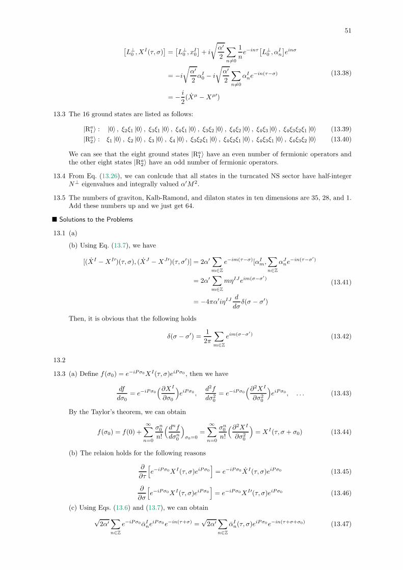
51

[

L⊥0 , X

I(τ, σ)]

=[

L⊥0 , x

I0

]

+ i

√

α′

2

∑

n6=0

1

ne−inτ

[

L⊥0 , α

In

]

einσ

= −i√

α′

2αI0 − i

√

α′

2

∑

n6=0

αIne

−in(τ−σ)

= − i

2(Xµ −Xµ′)

(13.38)

13.3 The 16 ground states are listed as follows:

|Ra1〉 : |0〉 , ξ2ξ1 |0〉 , ξ3ξ1 |0〉 , ξ4ξ1 |0〉 , ξ3ξ2 |0〉 , ξ4ξ2 |0〉 , ξ4ξ3 |0〉 , ξ4ξ3ξ2ξ1 |0〉 (13.39)

|Ra2〉 : ξ1 |0〉 , ξ2 |0〉 , ξ3 |0〉 , ξ4 |0〉 , ξ3ξ2ξ1 |0〉 , ξ4ξ2ξ1 |0〉 , ξ4ξ3ξ1 |0〉 , ξ4ξ3ξ2 |0〉 (13.40)

We can see that the eight ground states |Ra1〉 have an even number of fermionic operators and

the other eight states |Ra2〉 have an odd number of fermionic operators.

13.4 From Eq. (13.26), we can conlcude that all states in the turncated NS sector have half-integerN⊥ eigenvalues and integrally valued α′M2.

13.5 The numbers of graviton, Kalb-Ramond, and dilaton states in ten dimensions are 35, 28, and 1.Add these numbers up and we just get 64.


13.1 (a)

(b) Using Eq. (13.7), we have

[(XI −XI′)(τ, σ), (XJ −XJ′)(τ, σ′)] = 2α′∑

m∈Z

e−im(τ−σ)[αIm,

∑

n∈Z

αJne

−in(τ−σ′)

= 2α′∑

m∈Z

mηIJeim(σ−σ′)

= −4πα′iηIJd

dσδ(σ − σ′)

(13.41)

Then, it is obvious that the following holds

δ(σ − σ′) =1

2π

∑

m∈Z

eim(σ−σ′) (13.42)

13.2

13.3 (a) Define f(σ0) = e−iPσ0XI(τ, σ)eiPσ0 , then we have

df

dσ0= e−iPσ0

(∂XI

∂σ0

)

eiPσ0 ,d2f

dσ20

= e−iPσ0

(∂2XI

∂σ20

)

eiPσ0 , . . . (13.43)

By the Taylor’s theorem, we can obtain

f(σ0) = f(0) +

∞∑

n=0

σn0

n!

(dnf

dσn0

)

σ0=0=

∞∑

n=0

σn0

n!

(∂2XI

∂σ20

)

= XI(τ, σ + σ0) (13.44)

(b) The relaion holds for the following reasons

∂

∂τ

[

e−iPσ0XI(τ, σ)eiPσ0

]

= e−iPσ0XI(τ, σ)eiPσ0 (13.45)

∂

∂σ

[

e−iPσ0XI(τ, σ)eiPσ0

]

= e−iPσ0XI′(τ, σ)eiPσ0 (13.46)

(c) Using Eqs. (13.6) and (13.7), we can obtain

√2α′

∑

n∈Z

e−iPσ0 αIne

iPσ0e−in(τ+σ) =√2α′

∑

n∈Z

αIn(τ, σ)e

iPσ0e−in(τ+σ+σ0) (13.47)

52 CHAPTER 13. RELATIVISTIC QUANTUM CLOSED STRINGS

√2α′

∑

n∈Z

e−iPσ0αIne

iPσ0e−in(τ−σ) =√2α′

∑

n∈Z

αIn(τ, σ)e

iPσ0e−in(τ−σ−σ0) (13.48)

e−iPσ0 αIne

iPσ0 = αIne

−inσ0 , e−iPσ0αIne

iPσ0 = αIne

inσ0 (13.49)

(d) Using the reults above, we have

e−iPσ0 |U〉 = (e−iPσ0αI−me

iPσ0)(eiPσ0 αI−ne

iPσ0 ) |U〉 = αI−mα

I−ne

−i(m−n)σ0 |U〉 (13.50)

The invariance of |U〉 under σ0 transformation requires σ0 = 2kπ.

13.4 (a) Using Eq. (13.12), we can obtain

∫ 2π

0

dσXIXI′ = α′∑

n∈Z

∫ 2π

0

dσ e−inτ (L⊥n − e−inσ − L⊥

n einσ) = 2πα′(L⊥

0 − L⊥0 ) (13.51)

13.5

13.6

13.7 (a) bi1bi2 : 8× 7 + 1 = 57. bi1bi2bi3 : 8× 7× 6 + 1 = 337. bi1bi2bi3bi4 : 8× 7× 6× 5 + 1 = 1681.

Part II

DEVELOPMENTS

53

Chapter 14

D-branes and Gauge Fields


1. Quantizing open strings on Dp-branes

DD: Xa(τ, σ)∣

∣

σ=0= Xa(τ, σ)

∣

∣

σ=π= xa, a = p+ 1, . . . , d (14.1)

NN: Xm′(τ, σ)∣

∣

σ=0= Xm′(τ, σ)

∣

∣

σ=π= 0, m = 0, 1, . . . , p (14.2)

(14.3)

(14.4)

(14.5)

2.(14.6)

(14.7)

3.(14.8)

(14.9)

Quick Calculations

14.1

14.2

14.3


14.1

14.2

14.3

55

56 CHAPTER 14. D-BRANES AND GAUGE FIELDS

Appendices

57

Appendix A

Elements of E8

A.1 Introduction

Source from: http://en.wikipedia.org/wiki/E8 (mathematics)

In mathematics, E8 is the name given to several closely related exceptional simple Lie groups and Liealgebras of dimension 248; the same notation is sometimes used for their root lattice, which has rank 8.The designation E8 comes from Killing and Cartan’s classification of the complex simple Lie algebras,which fall into four infinite families labeled An, Bn, Cn, Dn, and five exceptional cases labeled E6, E7,E8, F4, and G2. The E8 algebra is the largest and most complicated of these exceptional cases.

The E8 Lie group has applications in theoretical physics, in particular in string theory and supergravity.The group E8 × E8 serves as the gauge group of one of the two types of heterotic string and is one oftwo anomaly-free gauge groups that can be coupled to the N = 1 supergravity in 10 dimensions. E8

is the U-duality group of supergravity on an eight-torus (in its split form). One way to incorporatethe standard model of particle physics into heterotic string theory is the symmetry breaking of E8 toits maximal subalgebra SU(3) × E6. In 1982, Michael Freedman used the E8 lattice to construct anexample of a topological 4-manifold, the E8 manifold, which has no smooth structure. In February2008, Garret Lisi published a particle physics theory based on the E8 Lie group.

59

http://en.wikipedia.org/wiki/E8_(mathematics)

60 APPENDIX A. ELEMENTS OF E8

Appendix B

Modular Forms

B.1 Introduction

Source from: http://en.wikipedia.org/wiki/Modular form

In mathematics, a modular form is a (complex) analytic function on the upper half-plane satisfyinga certain kind of functional equation and growth condition. The theory of modular forms thereforebelongs to complex analysis but the main importance of the theory has traditionally been in itsconnections with number theory. Modular forms appear in other areas, such as algebraic topology andstring theory. A modular function is a modular form of weight 0: it is invariant under the modulargroup, instead of transforming in a prescribed way, and is thus a function on the modular region (ratherthan a section of a line bundle). Modular form theory is a special case of the more general theory ofautomorphic forms, and therefore can now be seen as just the most concrete part of a rich theory ofdiscrete groups.

61

http://en.wikipedia.org/wiki/Modular_form

62 APPENDIX B. MODULAR FORMS

Bibliography

[1] B. Zwiebach, A First Course in String Theory. Cambridge University Press, 2004.

[2] M.B. Green, J.H. Schwarz, and E. Witten, Superstring Theory, Volume 1: Introduction. CambridgeUniversity Press, 1987.

63

Answers to Zwei 2010

Documents

Transcript of Answers to Zwei 2010