Answers to Exercises for Chapter 17 INTRODUCTION TO · PDF fileINTRODUCTION TO COMPUTER...

D-4415-5 1

Answers to Exercises for Chapter 17 INTRODUCTION TO DELAYS from

INTRODUCTION TO COMPUTER SIMULATION written by

Nancy RobertsDavid F. AndersenJonathan ChoateRalph M. Deal

Michael S. GaretWilliam A. Shaffer

Models translated to STELLA II 3.0 and Answers provided by

Kamil MseferMark Choudhari

Prepared forMIT System Dynamics Education Project

Under the Supervision ofDr. Jay W. Forrester

System Dynamics GroupSloan School of Management

August 5, 1994Vensim Examples added October 2001

Copyright © 2001 by the Massachusetts Institute of TechnologyPermission granted for non-commercial educational purposes

2 D-4415-5

INTRODUCTION TO COMPUTER SIMULATION can be ordered from Productivity Press, Inc., Dept. 315 P.O. Box 13390, Portland, OR 97213

The Chapter has also been provided under Road Maps Five in pdf format.

4 D-4415-5

Please read Chapter 17: Introduction to Delays from Introduction to

Computer Simulation by Nancy Roberts et. al. However, the chapter in the book

has its models built using the DYNAMO simulation language, and as you are

probably using Vensim, STELLA or iTHINK, we have translated the models for

your convenience. This paper contains these translated versions of the models for

the first seven exercises from the book. Later, we also suggest answers to these

exercises for you to measure your answers against.

NOTE FROM THE TRANSLATOR: All the models in this paper have rates that flow in both directions. This is to encourage the readers to make the direction of the flow explicit in the equation, and not in the plumbing. In DYNAMO, there is no biflow-uniflow toggle. All rates are biflows.

Example 1: The Martan Chemical Company

We present the model of dumping of the Nobug pesticide by the Martan

Chemical Company, as translated from DYNAMO to STELLA. A causal loop and

flow diagram of the Martan case are shown in Figure 1.

The equations for the model are as follows:

NOBUG(t) = NOBUG(t - dt) + (Dump_rate - Absorb_rate) * dtINIT NOBUG = 0

OUTFLOWS:ABSORB_RATE = NOBUG/NAT

NAT = 2

D-4415-5 5

NOBUG

DUMP RATE ABSORB RATE

NOBURG ABSORP TIME

Figure 1. Diagram of the Martan Case

These equations show that the level of NOBUG in the Sparkill River is

influenced by the DUMP RATE and the ABSORB RATE; and the ABSORB RATE

is equal to the level of NOBUG divided by the Nobug Absorption Time NAT (2

days).

Exercise 1: Preliminary Nobug Model

a. Create a STELLA II model for the Nobug case, adding the DUMP RATE

equation, and other needed specifications. Run the model, setting the initial level of

NOBUG = 0 and choosing DT = 0.25 days. Set length of simulation (in the Time

specs window under the Run menu) to 25 days, the range of Nobug (in the Range

specs window under the Run menu) from 0 to 250 gallons and the range of the

absorption rate from 0 to 100 gallons/day. What behavior does the model generate?

6 D-4415-5

b. Rerun the model, setting the Nobug Absorption Time, NAT = 4. How do the

results differ? Rerun the model, setting NAT = 1. How do these results differ?

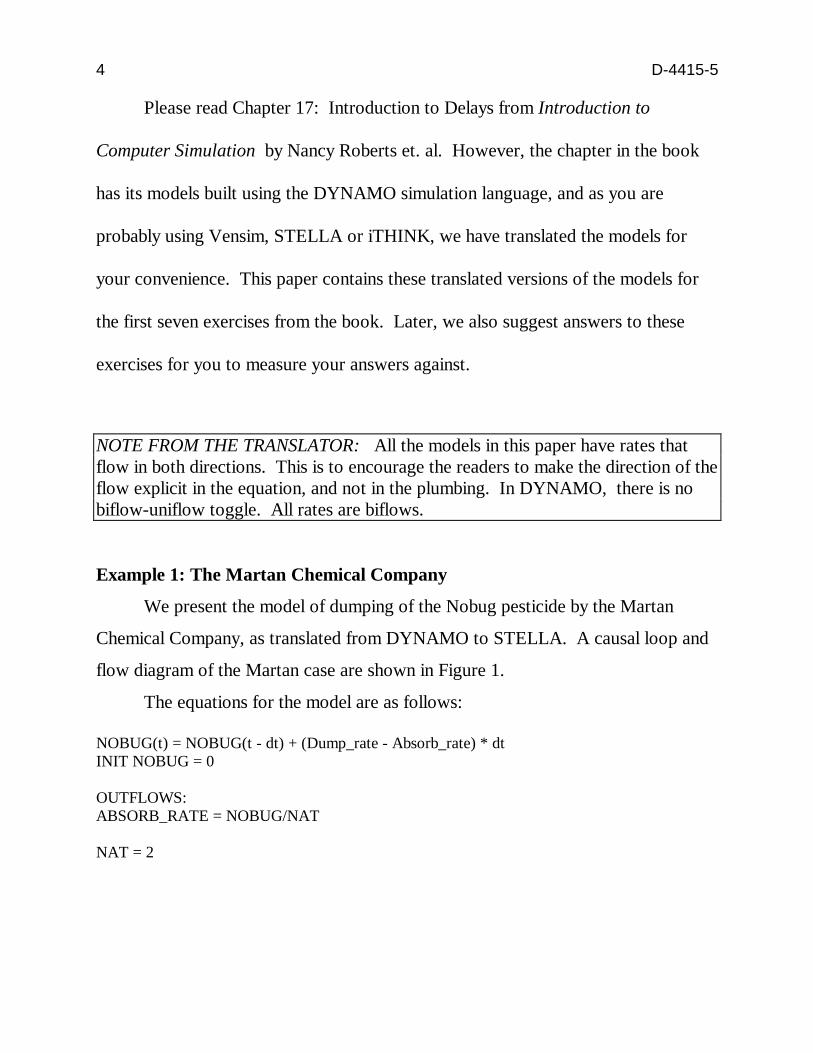
USING THE PULSE FUNCTION TO REPRESENT THE DUMPING RATE

We use the corresponding STELLA functions instead of the DYNAMO

functions in these exercises. The STELLA PULSE function permits modifying the

model to represent the dumping of Nobug in once a week batches. The following

rate equation indicates that 420 gallons of Nobug are dumped into the river on day 1

of the simulation, and 420 are dumped again at regular intervals of 7 days.

DUMP RATE = PULSE(420,1,7)

Figure 2 shows the dumping rate over the first 25 days of the simulation. Please see

the chapter in the book for further reading.

1: DUMP RATE 1: 1680.00

1: 840.00

1: 0.00 1 1 1 1 0.00 6.25 12.50 18.75 25.00

Graph 3 Days 6:32 PM 7/25/94

Figure 2. Dumping rate

The PULSE function can also be used to examine the response of the system

D-4415-5 7

to the dumping of just one batch of NOBUG. It is possible to do this by making the

following change in the equation for DUMP RATE.

DUMP RATE = PULSE(420,1,0)

This equation indicates that the dumping rate rises from zero to 1680 on day

one (for only a quarter of the day)and stays at zero for the rest of the simulation.

Figure 3 shows a simulation of the Nobug system, with one batch of Nobug

released into the river on day one. As can be seen, the level of NOBUG in the river

rises sharply to 420 gallons on day one, and then drifts slowly toward zero.

1: DUMP RATE 2: NOBUG 3: ABSORB RATE 1: 2000.00 2: 500.00 3: 250.00

1: 1000.00 2: 250.00 3: 125.00

1: 0.00 2: 0.00 3: 0.00 1 2

3

1

2 3

1

2 3 1 2 3

0.00 2.50 5.00 7.50 10.00

Graph 3 Days 6:43 PM 7/25/94

Figure 3. Release of one batch of NOBUG

The general form of the PULSE function is

PULSE(AMOUNT, FIRST, INTERVAL)

where AMOUNT indicates the amount to be inputted in the pulse; FIRST indicates

the time at which the first pulse occurs; and INTERVAL indicates the time interval

between pulses. Setting INTERVAL to 0, indicates to STELLA that you only want

8 D-4415-5

one pulse.

Exercise 2: The Halving Time for NOBUG

Revise your STELLA equations to include a PULSE function for the DUMP RATE.

Choose an interval of 0, in order to examine the effects of just one pulse.

a. What is the halving time for the amount of NOBUG in the Sparkill River?

b. Experiment with various values of NAT. How does the choice of NAT influence

the halving time?

c. Using your result for part (b), select a value of NAT to produce a halving time

that corresponds to the data shown below in Figure 4.

Exercises 3: Simulating Repeated Batches

a. Select NAT equal to the value you determined in Exercise 2, part (c). Use the

D-4415-5 9

PULSE function to simulate the effect of dumping 420 gallons of Nobug into the

river at 7-day intervals. Compare your results with the data shown in , Figure 4

above.

b. Assume Martan Chemical Inc. changed the chemical composition of Nobug,

such that the halving time of Nobug was lengthened to seven days, resulting in an

increase in the Nobug absorption time NAT. Change the value of NAT in your

model to reflect the change in the chemical composition of Nobug. How does the

system respond?

NOBUG AND MATERIAL DELAYS

Please read the chapter for an introduction to the concept of a first-order

material delay. LEVEL

INFLOW OUTFLOW

ADJUSTMENT TIME

Figure 5. First-order material delay

When a first-order material delay is used in a model, there are two ways to

write the equations. One approach is to simply to write out individual equations,

exactly as was done in the Nobug case. But because first-order material delays are

frequently used, a special STELLA function is available that can be used to replace

the set of individual equations. Note that we are using the equivalent STELLA

functions instead of the DYNAMO functions used in the book. The following

equation can be used to indicate that the OUTFLOW rate is a first-order delayed

response to the INFLOW rate, with an adjustment AT.

10 D-4415-5

OUTFLOW = SMTH1(INFLOW, AT)

LEVEL

INFLOW OUTFLOW

Figure 6. First-order material delay using SMTH1 function.

The SMTH1 function is simply a shorthand notation. When the model is run,

STELLA will substitute the full level and rate formulation for a first-order delay,

whenever the SMTH1 function appears in the model.

NOTE FROM THE TRANSLATOR: Exercise 4 from the original text has been left out intentionally.

Exercise 5: The Mail Delay

The Nifty Department Store sends out bills to its charge-card customers once a

month, and the credit department has learned that on the average, it takes about

three days for the bills to arrive in the mail.

a. Draw a causal-loop diagram, flow diagram, and equations for the Nifty

Department Store case. (Hint: See figure 7). Assume that NIFTY has 1000 charge

customers.

b. Run the Model and examine the results.

c. How many bills take more than six days to arrive?

D-4415-5 11

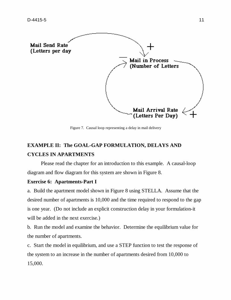
Figure 7. Causal loop representing a delay in mail delivery

EXAMPLE II: The GOAL-GAP FORMULATION, DELAYS AND

CYCLES IN APARTMENTS

Please read the chapter for an introduction to this example. A causal-loop

diagram and flow diagram for this system are shown in Figure 8.

Exercise 6: Apartments-Part I

a. Build the apartment model shown in Figure 8 using STELLA. Assume that the

desired number of apartments is 10,000 and the time required to respond to the gap

is one year. (Do not include an explicit construction delay in your formulation-it

will be added in the next exercise.)

b. Run the model and examine the behavior. Determine the equilibrium value for

the number of apartments.

c. Start the model in equilibrium, and use a STEP function to test the response of

the system to an increase in the number of apartments desired from 10,000 to

15,000.

12 D-4415-5

Apartments

Construction Rate

Apartments Desired

Adjustment Rate Gap

Figure 8. Diagrams expressing a housing gap

Please read the chapter for a discussion of why a delay should be added to the

model. One way to do this is shown in figure 9.

Apartments in Construction Total # of Apartments

Initiation Rate Completion Rate

Initiation Time Completion Time CT

Desired ApartmentsDifference

Figure 9. Apartment model with completion delay

D-4415-5 13

Exercise 7: Apartments-Part II

For the questions in this exercise, please refer to the chapter.

INFORMATION DELAYS

Please read the chapter for an introduction to information delays.

EXAMPLE III: MARINA’S BAKE SHOP

Please read the chapter for an introduction to Marina and her Bake Shop.

NOTE FROM THE TRANSLATOR: This paper presents only the first seven exercises from Chapter 7 in the book. We will discuss higher order delays later in Road Maps.

Now, we present our suggestions for the answers to the exercises.

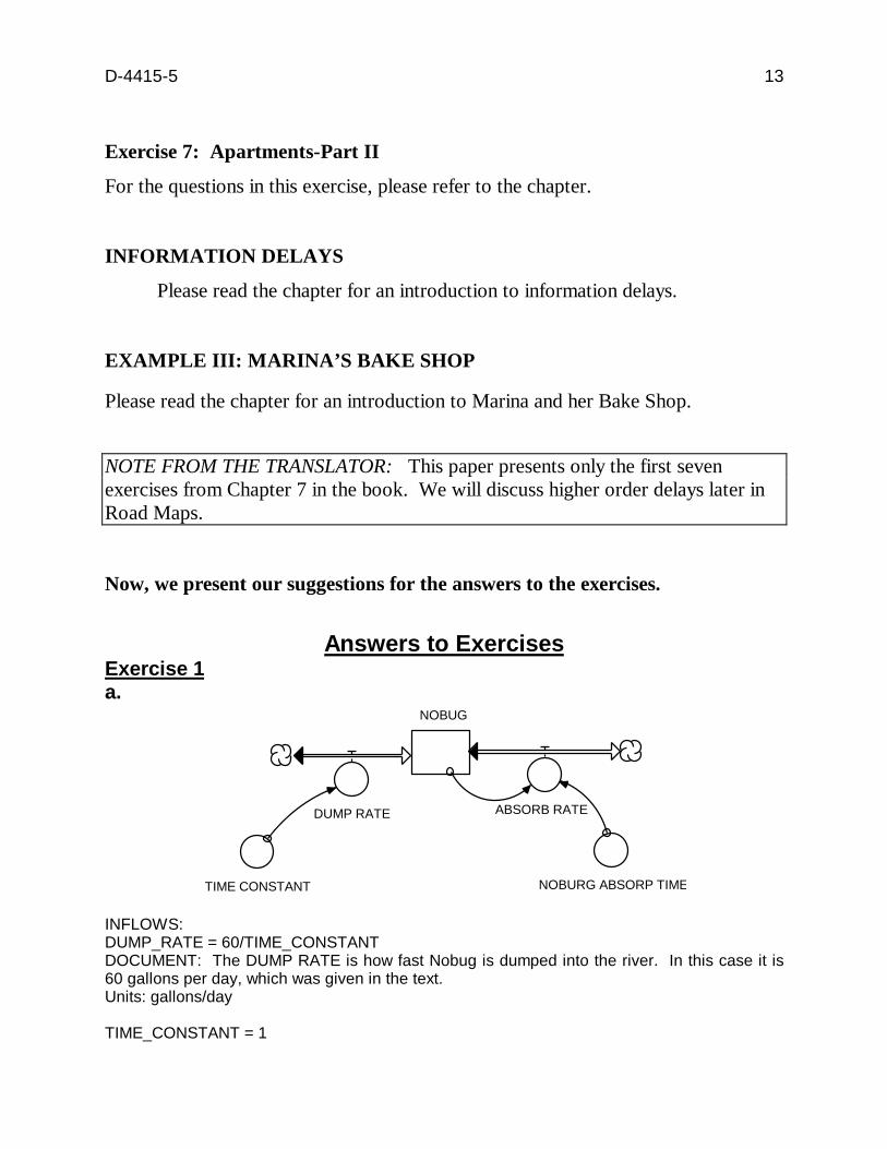
Answers to Exercises Exercise 1 a.

NOBUG

DUMP RATE ABSORB RATE

TIME CONSTANT NOBURG ABSORP TIME

INFLOWS: DUMP_RATE = 60/TIME_CONSTANT DOCUMENT: The DUMP RATE is how fast Nobug is dumped into the river. In this case it is 60 gallons per day, which was given in the text. Units: gallons/day

TIME_CONSTANT = 1

14 D-4415-5

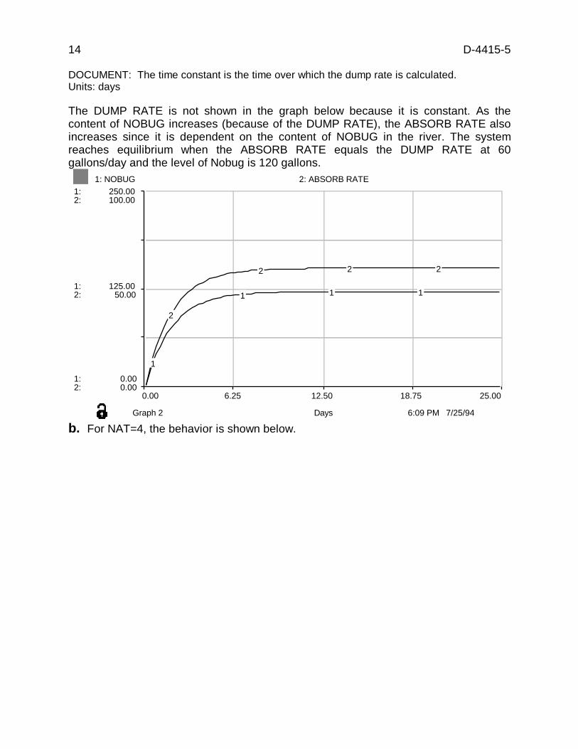
DOCUMENT: The time constant is the time over which the dump rate is calculated. Units: days

The DUMP RATE is not shown in the graph below because it is constant. As the content of NOBUG increases (because of the DUMP RATE), the ABSORB RATE also increases since it is dependent on the content of NOBUG in the river. The system reaches equilibrium when the ABSORB RATE equals the DUMP RATE at 60 gallons/day and the level of Nobug is 120 gallons.

1: NOBUG 2: ABSORB RATE 1: 250.00 2: 100.00

1: 125.00 2: 50.00

1: 0.00 2: 0.00

1

2

1

2

1

2

1

2

0.00 6.25 12.50 18.75 25.00

Graph 2 Days 6:09 PM 7/25/94

b. For NAT=4, the behavior is shown below.

D-4415-5 15


1: 125.00 2: 50.00

1: 0.00 2: 0.00

1

2

1

2

1

2

1

2

0.00 6.25 12.50 18.75 25.00

Graph 2 Days 6:16 PM 7/25/94

When NAT=4, it takes twice as long to reach equilibrium, because the ABSORB RATE is twice as small as in part a. Also, the new equilibrium level of Nobug is at 240 gallons.

For NAT=1, the behavior is shown below. 1: NOBUG 2: ABSORB RATE

1: 250.00 2: 100.00

1: 125.00 2: 50.00

1: 0.00 2: 0.00

1

2

1

2

1

2

1

2

0.00 6.25 12.50 18.75 25.00

Graph 2 Days 6:23 PM 7/25/94

When NAT=1, equilibrium is reached in half the time it takes in part a. That is because the ABSORB RATE is twice as large as in part a. The new equilibrium level of Nobug is at 60 gallons.

16 D-4415-5

Exercise 2 a. The level of NOBUG drops from 420 gallons at day 1 to about 210 gallons in 2.5 days. The halving time is then about 1.5 days.

b. After experimentation, you should find that an increase or decrease in the Nobug Absorption Time correspondingly increases or decreases the halving time.

c. Figure 4 shows a halving time for NOBUG of about 1 day (ie. half-life = 1 day). The value of NAT that produces this behavior can be calculated as (half-life)/.69 or 1.4 days. With this value for NAT the outcome matches Figure 4.

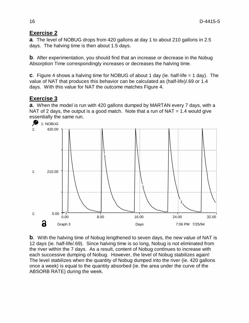
Exercise 3 a. When the model is run with 420 gallons dumped by MARTAN every 7 days, with a NAT of 2 days, the output is a good match. Note that a run of NAT = 1.4 would give essentially the same run.

1: NOBUG 1: 420.00

1: 210.00

1: 0.00 1

1

1

1

0.00 8.00 16.00 24.00 32.00

Graph 3 Days 7:06 PM 7/25/94

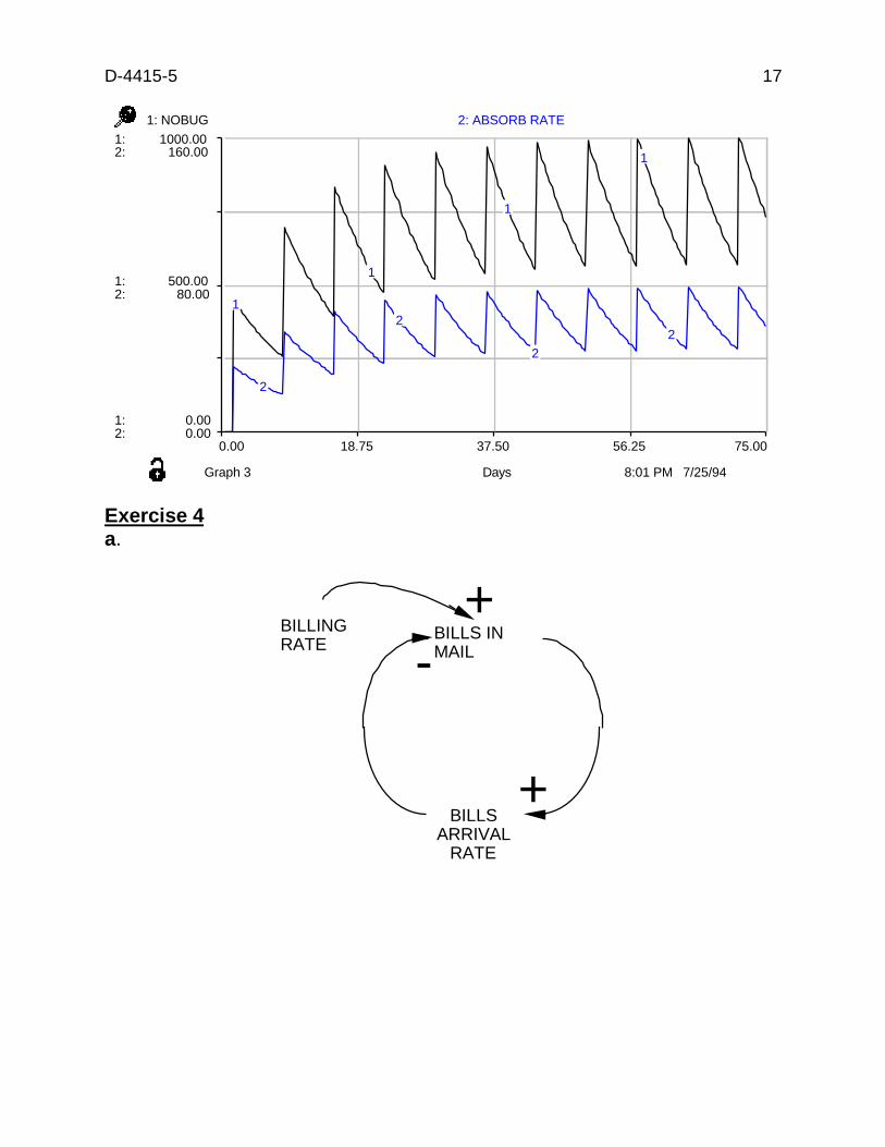
b. With the halving time of Nobug lengthened to seven days, the new value of NAT is 12 days (ie. half-life/.69). Since halving time is so long, Nobug is not eliminated from the river within the 7 days. As a result, content of Nobug continues to increase with each successive dumping of Nobug. However, the level of Nobug stabilizes again! The level stabilizes when the quantity of Nobug dumped into the river (ie. 420 gallons once a week) is equal to the quantity absorbed (ie. the area under the curve of the ABSORB RATE) during the week.

D-4415-5 17


1: 500.00 2: 80.00

1: 0.00 2: 0.00

1

2

1

2

1

2

1

2

0.00 18.75 37.50 56.25 75.00

Graph 3 Days 8:01 PM 7/25/94

Exercise 4 a.

ARRIVAL RATE

BILLS IN MAIL

BILLS

BILLING RATE -

+

+

18 D-4415-5

Bills in the mail Bills received

Billing Rate Bill Arrival Rate

Mail Arrival Delay

Bills_in_the_mail(t) = Bills_in_the_mail(t - dt) + (Billing_Rate - Bill_Arrival_Rate) * dtINIT Bills_in_the_mail = 0DOCUMENT: Initially there are no bills in the mail.Units: bills

INFLOWS:Billing_Rate = PULSE(1000,1,0)DOCUMENT: 1000 bills are sent out on the first day of the month. The interval was set to 0because in this case we are only interested in studying the first pulse.Units: bills/day

OUTFLOWS:Bill_Arrival_Rate = Bill_Arrival_Rate/Mail_Arrival_DelayDOCUMENT: This is a first order material delay, where bills arrive on average 3 days afterthey are sent.Units: bills/days.

Mail_Arrival_Rate = 3Document : Time it takes for mail to arrive to destination.Units: days

Another way of modeling the same behavior using the SMTH1 function is shown below. The behavior of this model should be the same as the graph below.

Bills in the mail Bills received

Billing Rate Bill Arrival Rate

Billing_Rate = PULSE(1000,1,0)Bill_Arrival_Rate = SMTH1(Billing_Rate, 3)DOCUMENT: The adjustment time or delay is 3 days.

b.

D-4415-5 19

1: Bills received 2: Bill Arrival Rate 1: 1000.00 1 2: 333.33

1: 500.00 2: 166.67

1: 0.00 2: 0.00 1

2 1

2

1

2 2 0.00 5.00 10.00 15.00 20.00

Graph 1 Days 3:11 PM 7/26/94

The pattern in the output is a mail arrival rate that decays exponentially from an initial peak just after the mail is sent. This is an unrealistic modeling of the mail process since no mail will be received immediately after the mail is sent.

c. From the tabular output, at the end of 6 days, 806 bills have been received or 194 bills (ie. 1000-806) will take more than 6 days to arrive.

Exercise 6 a.

Apartments

Construction Rate Apartments Desired

Adjustment Rate

Gap

Apartments(t) = Apartments(t - dt) + (Construction_Rate) * dtINIT Apartments = 0

DOCUMENT: Apartments built so far.Units: apartments

INFLOWS:Construction_Rate = Gap/Adjustment_Rate

20 D-4415-5

DOCUMENT: Apartments per year constructed.Units: apartments/year

Adjustment_Rate = 1DOCUMENT: Time to respond to the gap is one year.Units : years

Apartments_Desired = 10000DOCUMENT: Units : apartments

Gap = Apartments_Desired-ApartmentsDOCUMENT: Difference between the number of desired apartments and actual apartments.Units: apartments.

b. 1: Construction Rate 2: Apartments

1: 10000.00 2 2:

1: 5000.002:

1: 2: 0.00

1

2

1

2

1

2

1 0.00 1.50 3.00 4.50 6.00

Graph 2 Years 3:42 PM 7/26/94

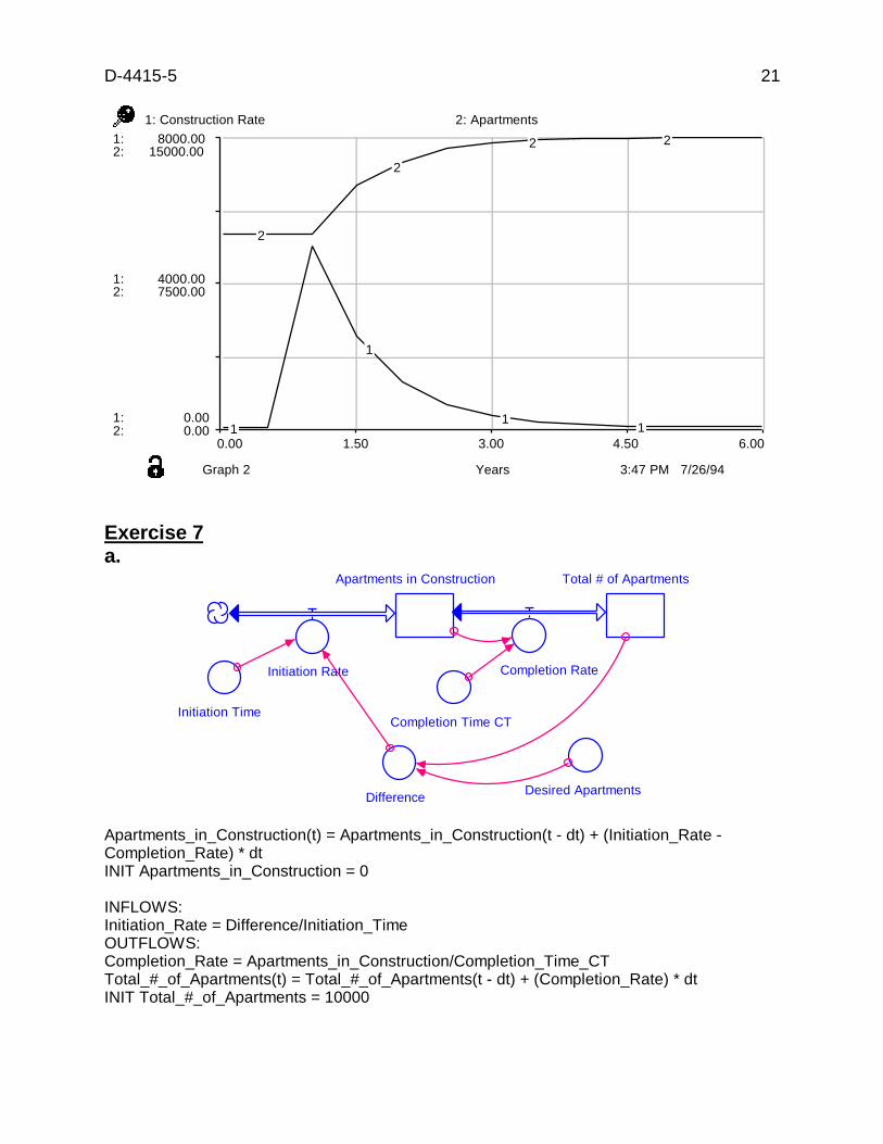
From the plot, the number of apartments at equilibrium will be 10000, as expected for this simple model with no demolition process.

c. The equation for desired apartments should be changed to: Apartments_Desired = 10000 + STEP( 5000,1)

2

D-4415-5 21

1: Construction Rate 2: Apartments 1: 8000.00 2: 15000.00

1: 4000.00 2: 7500.00

1: 0.00 2: 0.00 1

2

1

2

1

2

1 0.00 1.50 3.00 4.50 6.00

Graph 2 Years 3:47 PM 7/26/94

Exercise 7 a.

Apartments in Construction Total # of Apartments

Initiation Rate Completion Rate

Initiation Time Completion Time CT

Difference Desired Apartments

Apartments_in_Construction(t) = Apartments_in_Construction(t - dt) + (Initiation_Rate Completion_Rate) * dt INIT Apartments_in_Construction = 0

INFLOWS: Initiation_Rate = Difference/Initiation_Time OUTFLOWS: Completion_Rate = Apartments_in_Construction/Completion_Time_CT Total_#_of_Apartments(t) = Total_#_of_Apartments(t - dt) + (Completion_Rate) * dt INIT Total_#_of_Apartments = 10000

22 D-4415-5

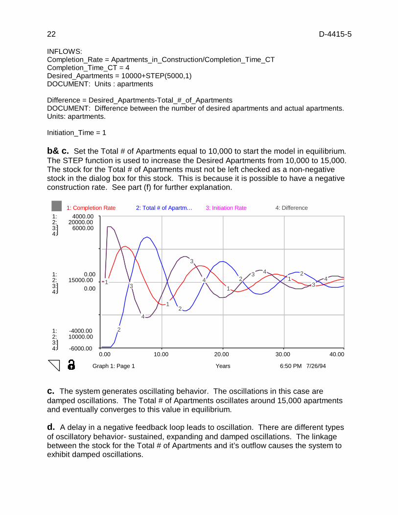
INFLOWS:Completion_Rate = Apartments_in_Construction/Completion_Time_CTCompletion_Time_CT = 4Desired_Apartments = 10000+STEP(5000,1)DOCUMENT: Units : apartments

Difference = Desired_Apartments-Total_#_of_ApartmentsDOCUMENT: Difference between the number of desired apartments and actual apartments.Units: apartments.

Initiation_Time = 1

b& c. Set the Total # of Apartments equal to 10,000 to start the model in equilibrium. The STEP function is used to increase the Desired Apartments from 10,000 to 15,000. The stock for the Total # of Apartments must not be left checked as a non-negative stock in the dialog box for this stock. This is because it is possible to have a negative construction rate. See part (f) for further explanation.

1: Completion Rate 2: Total # of Apartm… 3: Initiation Rate 4: Difference 1: 4000.00 2: 20000.00 3: 6000.00 4:

1: 0.00 2: 15000.00 3: 0.004:

1: -4000.00 2: 10000.00 3: 4: -6000.00

1

2

3

4

1 2

3

4 1

2 3 4

1 2

3 4

0.00 10.00 20.00 30.00 40.00

Graph 1: Page 1 Years 6:50 PM 7/26/94

c. The system generates oscillating behavior. The oscillations in this case are damped oscillations. The Total # of Apartments oscillates around 15,000 apartments and eventually converges to this value in equilibrium.

d. A delay in a negative feedback loop leads to oscillation. There are different types of oscillatory behavior- sustained, expanding and damped oscillations. The linkage between the stock for the Total # of Apartments and it’s outflow causes the system to exhibit damped oscillations.

D-4415-5 23

e. Try three runs with Completion Times CT of 3, 4, and 6 years. In all cases, the number of apartments will oscillate about the equilibrium value, the main effect of changing the construction delays time is to change the period of oscillation. An increase in the Completion Time increases the period of oscillation and makes it take longer for the system to achieve equilibrium. In all cases, the oscillations are damped, becoming smaller and smaller in amplitude from each cycle to the next.

f. A negative apartment construction rate appears to be physical nonsense. However, it could correspond to the destruction of buildings or to the cancellation of contracts to build, even after construction has started. The prediction was to be made for a period twice as long as your run. Since you have made several runs, you have several possibilities. Consider the case of CT (construction delay time) being 6 years. The period of oscillation for this value of CT is about 15 years so you could expect new maxima in the rate of completion of apartments at 35 and 50 years but much smaller in size than those at 5 and 20 years. A run for 50 years shows just that pattern.

24 D-4415-5

Nobug

dump rate absorb rate

NOBUG ABSORPTION

NOBUG/DAY

Vensim Examples: Introduction to Computer Simulation

By Lei Lei and Samitha Samaranayake October 2001

Example 1A: Martan Chemical Company

INITIAL NOBUG TIME

Figure 10: Vensim Equivalent of Diagram of the Martan Case without Pulse Function

Documentation for Martan Chemical Company Model

(01) absorb rate = Nobug/NOBUG ABSORPTION TIME Units: gallons/day

(02) dump rate = "NOBUG/DAY" Units: gallons/day The dump rate is how fast Nobug is dumped into the river.

(03) FINAL TIME = 25 Units: days The final time for the simulation.

(04) INITIAL NOBUG = 0 Units: gallons The Initial amount of Nobug is 0 gallons.

(05) INITIAL TIME = 0 Units: days The initial time for the simulation.

(06) Nobug = INTEG (+dump rate-absorb rate, INITIAL NOBUG) Units: gallons

(07) NOBUG ABSORPTION TIME = 1

D-4415-5 25

Units: day (08) "NOBUG/DAY" = 60

Units: gallons/day

(09) SAVEPER = TIME STEP Units: days The frequency with which output is stored.

(10) TIME STEP = 0.25 Units: days The time step for the simulation.

Graph of Nobug and Absorb Rate for NAT=2 2 250 gallons

100 gallons/day

125 gallons 50 gallons/day


2 2 2 2 2 2 2 2

1 1 1 1 1 1 1 1

2

1

1

0 5 10 15 20 25 Time (days)

Nobug : current 1 1 1 1 1 1 1 gallons absorb rate : current 2 2 2 2 2 gallons/day

Figure 11: Vensim Equivalent of Simulation for NAT = 2

1

26 D-4415-5


100 gallons/day



1 1 1 1 1 1

1 2

1

2 2 2 2 2

2 2

2 1

0 5 10 15 20 25 Time (days)




100 gallons/day



1

0 5 10 15 20 25 Time (days)


2 2 2 2 2 2 2 2

2

1

1 1 1 1 1 1 1 1


D-4415-5 27

Example 1B: Dump Rate With Pulse(s)

Nobug dump rate absorb rate

NOBUG ABSORPTION TIME <TIME STEP>

NOBUG/DAY

INITIAL NOBUG Figure 14: Vensim Equivalent of Figure 1: Diagram of Martan Case

Documentation for Dump Rate With Pulse(s) Model

(01) absorb rate = Nobug/NOBUG ABSORPTION TIME Units: gallons/day

(02) dump rate = "NOBUG/DAY"*( PULSE(1 ,TIME STEP)+ PULSE(8 ,TIME STEP)+ PULSE(15 ,TIME STEP)+ PULSE(22 ,TIME STEP)) Units: gallons/day 420 gallons of Nobug are dumped each quarter of a day, so 1680 gallons of Nobug are dumped on the first day of each week

Note: This formulation is used because Vensim does not have a repeated pulses function. We have inserted individual pulses at intervals of 7 days instead.

(03) FINAL TIME = 25 Units: days The final time for the simulation.

(04) INITIAL NOBUG = 0 Units: gallons

(05) INITIAL TIME = 0 Units: days The initial time for the simulation.

(06) Nobug = INTEG (+dump rate-absorb rate, INITIAL NOBUG) Units: gallons

(07) NOBUG ABSORPTION TIME = 7 Units: day

(08) "NOBUG/DAY" = 1680 Units: gallons/day

28 D-4415-5

There are 1680 gallons of Nobug dumped per day.

(09) SAVEPER = TIME STEP Units: days The frequency with which output is stored.

(10) TIME STEP = 0.25 Units: day The time step for the simulation.

Graph for dump rate 1,680

840

0 1 11 1

1

1 1 1 1 1 1 1 1 0 4 8 12 16 20 24 28 32

Time (days)

dump rate : current 1 1 1 1 1 1 1 gallons/day

Figure 15: Vensim Equivalent of Figure 2: Simulation for dump rate

D-4415-5 29

Graph of Dump rate, Nobug, and Absorb Rate for One Pulse

2,000 gallons/day 500 gallons 250 gallons/day

1,000 gallons/day 250 gallons 125 gallons/day

0 gallons/day 0 gallons 0 gallons/day

3

2 3

32 2 3 2 3 32 2 3 32 32 2 3 32 21 31 2 1 1 1 1 1 1 1 1 1 1

0 4 8 12 16 20 24 28 32 Time (days)

dump rate : current 1 1 1 1 1 1 1 1 1 gallons/day Nobug : current 2 2 2 2 2 2 2 2 2 2 gallons absorb rate : current 3 3 3 3 3 3 3 3 3 gallons/day

Figure 16: Vensim Equivalent of Figure 3: Simulation of release of one batch of Nobug

Graph for Nobug 421.70

316.28

210.85

105.42

0

1 1

1

1

1

1 1

1 1

1 1

1

1

1

1 0 4 8 12 16 20 24 28 32

Time (days)

Nobug : current 1 1 1 1 1 1 1 1 1 1 gallons

Figure 17: Vensim Equivalent of Simulation of Nobug for NAT = 1.4

30 D-4415-5

Graph of Nobug and Absorb Rate for NAT = 12

1 0 10 20 30 40 50 60 70

Time (days)

Nobug : current 1 1 1 1 1 1 1 1 1 1 gallons absorb rate : current 2 2 2 2 2 2 2 2 2 gallons/day

Figure 18: Vensim Equivalent of Simulation of Nobug and Absorb Rate for NAT = 12

Exercise 5: The Mail Delay

INITIAL BILLS IN THE MAIL INITIAL BILLS RECEIVED

1,000 gallons 160 gallons/day



1 1

1 1

1

1 1

1 1

2 1

1 2

2 2 2 2 2 2 2 2

2 2

Bills in the Mail Bills Received bill arrival ratebilling rate

<TIME STEP>

MAIL ARRIVAL

BILLS/DAY

DELAY Figure 19: Vensim Equivalent of Mail Delay Model

Documentation for Mail Delay Model

(01) bill arrival rate = Bills in the Mail/MAIL ARRIVAL DELAY Units: bills/day This is a first order material delay, where bills arrive on average 3 days after they are sent.

D-4415-5 31

(02) billing rate = "BILLS/DAY"*PULSE(1, TIME STEP ) Units: bills/day 1000 bills are sent out on the first day of the month. The interval was set to 0 because in this case we are only interested in studying the first pulse.

(03) Bills in the Mail =INTEG (+billing rate-bill arrival rate, INITIAL BILLS IN THE MAIL) Units: bills Initially there are no bills in the mail.

(04) Bills Received = INTEG (bill arrival rate, INITIAL BILLS RECEIVED) Units: bills

(05) "BILLS/DAY"= 1000 Units: bills/day 1000 bills are sent out on the first day of the month.

(06) FINAL TIME = 20 Units: day The final time for the simulation.

(07) INITIAL BILLS IN THE MAIL = 0 Units: bills There are initially 0 Bills in the Mail.

(08) INITIAL BILLS RECEIVED = 0 Units: bills There are initially 0 bills received.

(09) INITIAL TIME = 0 Units: day The initial time for the simulation.

(10) MAIL ARRIVAL DELAY = 3 Units: day Time it takes for mail to arrive to destination.

(11) SAVEPER = TIME STEP Units: day The frequency with which output is stored.

(12) TIME STEP = 0.0625 Units: day The time step for the simulation.

32 D-4415-5

1 1 1

Graph of Bills Received and Bill Arrival Rate

2 11 0 2 4 6 8 10 12 14 16 18 20

Time (day)

Bills Received : current 1 1 1 1 1 1 1 1 1 1 bills bill arrival rate : current 2 2 2 2 2 2 2 2 2 bills/day

Figure 20: Vensim Equivalent of Simulation of Bills Received and Bill Arrival Rate

Exercise 6A: Apartments-Part 1

1,000 bills 333.32 bills/day

500 bills 166.66 bills/day

0 bills 0 bills/day

1 1

1 1 1 1 1

2

1

2

2

2 2 2 2 2 2 2 2

Apartments

ADJUSTMENT RATE gap

APARTMENTS DESIRED

construction rate

INITIAL APARTMENTS

Figure 21: Vensim Equivalent of Apartments Model-Part 1

Documentation for Apartments Model-Part 1

(01) ADJUSTMENT RATE = 1 Units: year Time to respond to the gap is one year.

(02) Apartments = INTEG (construction rate, INITIAL APARTMENTS)

D-4415-5 33

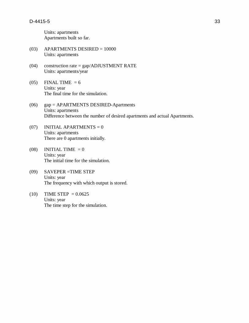
Units: apartments Apartments built so far.

(03) APARTMENTS DESIRED = 10000 Units: apartments

(04) construction rate = gap/ADJUSTMENT RATE Units: apartments/year

(05) FINAL TIME = 6 Units: year The final time for the simulation.

(06) gap = APARTMENTS DESIRED-Apartments Units: apartments Difference between the number of desired apartments and actual Apartments.

(07) INITIAL APARTMENTS = 0 Units: apartments There are 0 apartments initially.

(08) INITIAL TIME = 0 Units: year The initial time for the simulation.

(09) SAVEPER =TIME STEP Units: year The frequency with which output is stored.

(10) TIME STEP = 0.0625 Units: year The time step for the simulation.

34 D-4415-5

Graph for construction rate and Apartments With Step Function 2 2

1 1 0 1 2 3 4 5 6

Time (year)

construction rate : current 1 1 1 1 1 1 1 apartments/year Apartments : current 2 2 2 2 2 2 2 2 2 apartments

Figure 22: Vensim Equivalent of Simulation with Step Function

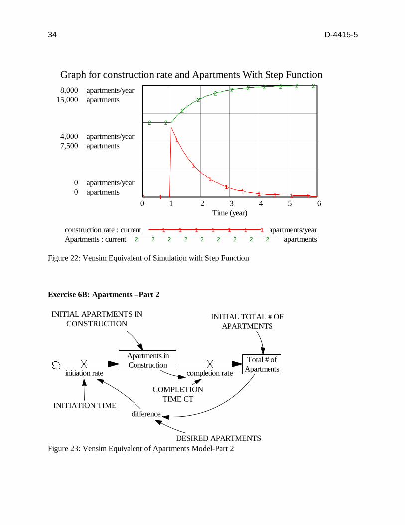
Exercise 6B: Apartments –Part 2

INITIAL APARTMENTS IN INITIAL TOTAL # OFCONSTRUCTION APARTMENTS

8,000 apartments/year 15,000 apartments

4,000 apartments/year 7,500 apartments

0 apartments/year 0 apartments

2

2 2 2 2 2 2

2 2

1

1

1 1

1 1 1 1 1

Apartments in Construction

Total # of Apartmentscompletion rateinitiation rate

INITIATION TIME

COMPLETION TIME CT

difference

DESIRED APARTMENTS Figure 23: Vensim Equivalent of Apartments Model-Part 2

D-4415-5 35

Documentation for Apartments Model-Part 2

(01) Apartments in Construction = INTEG (+initiation rate-completion rate, INITIAL APARTMENTS IN CONSTRUCTION)

Units: apartments

(02) completion rate = Apartments in Construction/COMPLETION TIME CT Units: apartments/year

(03) COMPLETION TIME CT = 4 Units: year

(04) DESIRED APARTMENTS = 10000+STEP(5000,1) Units: apartments

(05) difference = DESIRED APARTMENTS-"Total # of Apartments" Units: apartments Difference between the number of desired apartments and actual apartments.

(06) FINAL TIME = 40 Units: year The final time for the simulation.

(07) INITIAL APARTMENTS IN CONSTRUCTION = 0 Units: apartments There are 0 apartments initially.

(08) INITIAL TIME = 0 Units: year The initial time for the simulation.

(09) INITIAL TOTAL # OF APARTMENTS= 10000 Units: apartments There are 10000 apartments initially.

(10) initiation rate = difference/INITIATION TIME Units: apartments/year

(11) INITIATION TIME = 1 Units: year

(12) SAVEPER = TIME STEP Units: year The frequency with which output is stored.

(13) TIME STEP = 0.0625 Units: year

36 D-4415-5

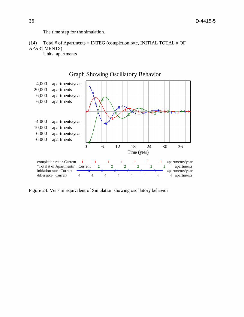
The time step for the simulation.

(14) Total # of Apartments = INTEG (completion rate, INITIAL TOTAL # OF APARTMENTS)

Units: apartments

Graph Showing Oscillatory Behavior 4,000 apartments/year

20,000 apartments 6,000 apartments/year 6,000 apartments

-4,000 apartments/year 10,000 apartments -6,000 apartments/year -6,000 apartments

3

1

4 1 2

3 4 1 3

21 4 3 4 21 32 4

3 4

2 1

2 4 3 1 2 43 1

2 0 6 12

Time (year) 18 24 30 36

completion rate : Current "Total # of Apartments" : initiation rate : Current

1 Current

3

1 2

3

1 2

3

1 2

3

1 2

3

1 2

3

1 2

apartments/year apartments

apartments/year difference : Current 4 4 4 4 4 4 4 4 apartments

Figure 24: Vensim Equivalent of Simulation showing oscillatory behavior

Answers to Exercises for Chapter 17 INTRODUCTION TO · PDF fileINTRODUCTION TO COMPUTER...

Documents

Transcript of Answers to Exercises for Chapter 17 INTRODUCTION TO · PDF fileINTRODUCTION TO COMPUTER...