1

Mixed Analysis of Variance Models with

SPSSRobert A.Yaffee, Ph.D.

Statistics, Social Science, and Mapping Group

Information Technology Services/Academic Computing Services

Office location: 75 Third Avenue, Level C-3Phone: 212-998-3402

2

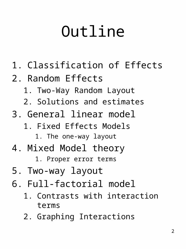
Outline

1. Classification of Effects2. Random Effects

1. Two-Way Random Layout2. Solutions and estimates

3. General linear model1. Fixed Effects Models

1. The one-way layout

4. Mixed Model theory1. Proper error terms

5. Two-way layout6. Full-factorial model

1. Contrasts with interaction terms2. Graphing Interactions

3

Outline-Cont’d

• Repeated Measures ANOVA• Advantages of Mixed Models

over GLM.

4

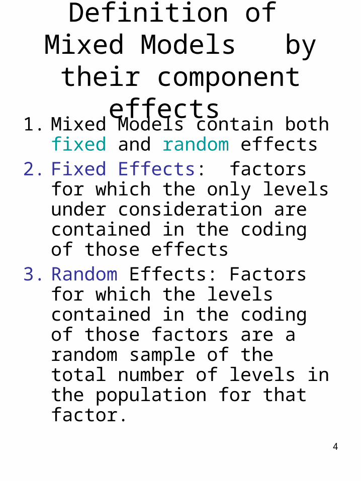
Definition of Mixed Models by their

component effects1. Mixed Models contain both

fixed and random effects2. Fixed Effects: factors for

which the only levels under consideration are contained in the coding of those effects

3. Random Effects: Factors for which the levels contained in the coding of those factors are a random sample of the total number of levels in the population for that factor.

5

Examples of Fixed and Random Effects

1. Fixed effect:2. Sex where both male and

female genders are included in the factor, sex.

3. Agegroup: Minor and Adult are both included in the factor of agegroup

4. Random effect: 1. Subject: the sample is a

random sample of the target population

6

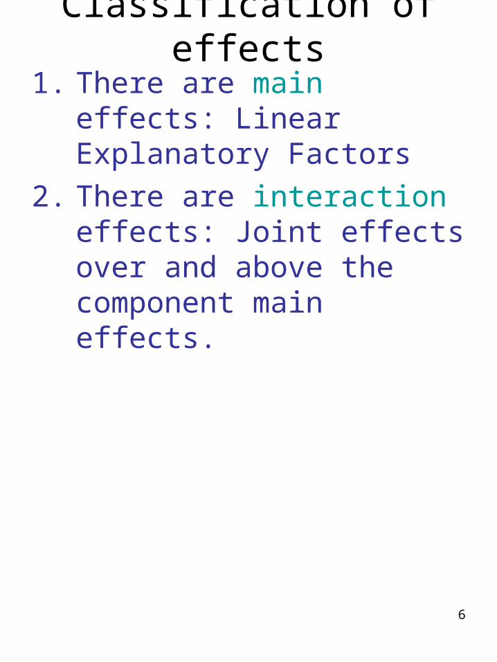
Classification of effects1. There are main effects:

Linear Explanatory Factors 2. There are interaction effects:

Joint effects over and above the component main effects.

7

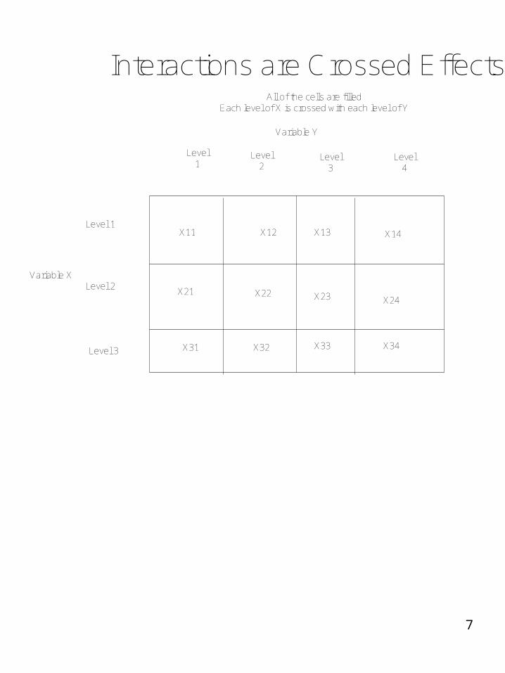
Interactions are Crossed Effects

Variable Y

Variable X

Level1

Level2

Level3

Level4

Level 1

Level 2

Level 3

X11 X12 X13 X14

X21 X22 X23 X24

X31 X32 X33 X34

All of the cells are filledEach level of X is crossed with each level of Y

8

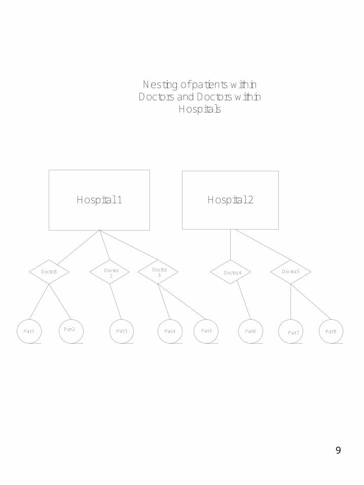
Classification of Effects-cont’d

Hierarchical designs have nested effects. Nested effects are those with subjects within groups.

An example would be patients nested within doctors and doctors nested within hospitals

This could be expressed bypatients(doctors)doctors(hospitals)

9

Hospital 1 Hospital 2

Doctor1 Doctor2

Doctor3 Doctor 4 Doctor 5

Pat 1 Pat 2 Pat 3 Pat 4 Pat 5 Pat 6 Pat 7 Pat 8

Nesting of patients withinDoctors and Doctors within

Hospitals

10

Between and Within-Subject effects

• Such effects may sometimes be fixed or random. Their classification depends on the experimental designBetween-subjects effects are those who are in one group or another but not in both. Experimental group is a fixed effect because the manager is considering only those groups in his experiment. One group is the experimental group and the other is the control group. Therefore, this grouping

factor is a between- subject effect. Within-subject effects are experienced by subjects repeatedly over time. Trial is a random effect when there are several trials in the repeated measures design; all subjects experience all of the trials. Trial is therefore a within-subject effect.Operator may be a fixed or random effect, depending upon whether one is generalizing beyond the sampleIf operator is a random effect, then the machine*operator interaction is a random effect.There are contrasts: These contrast the values of one level with those of other levels of the same effect.

11

Between Subject effects

• Gender: One is either male or female, but not both.

• Group: One is either in the control, experimental, or the comparison group but not more than one.

12

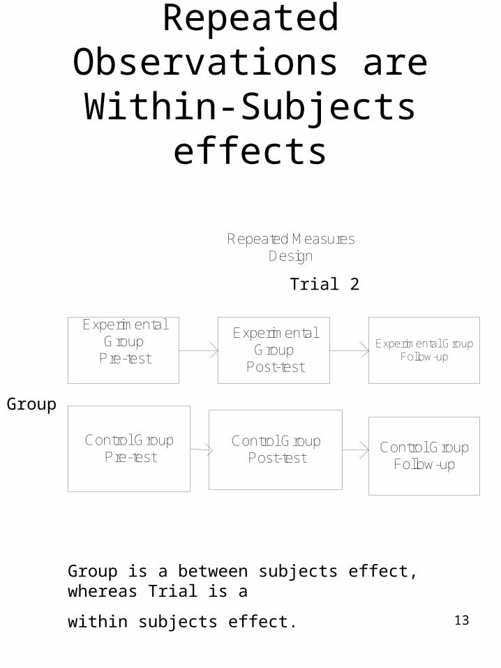
Within-Subjects Effects

• These are repeated effects.• Observation 1, 2, and 3 might

be the pre, post, and follow-up observations on each person.

• Each person experiences all of these levels or categories.

• These are found in repeated measures analysis of variance.

13

Repeated Observations are Within-Subjects

effects

ExperimentalGroup

Pre-test

Control GroupPre-test

ExperimentalGroup

Post-test

Control GroupPost-test

Experimental GroupFollow-up

Control GroupFollow-up

Repeated MeasuresDesign

Trial 1 Trial 2 Trial 3

Group

Group is a between subjects effect, whereas Trial is a

within subjects effect.

14

The General Linear Model

1. The main effects general linear model can be parameterized as

( )( )

( )

exp ~ ( , )

ij i j ij

ij

i i

j j

ij

Y b

whereY observation for ith

grand mean an unknown fixed parmeffect of ith value of a

b effect of jth value of b b

erimental error N

20

15

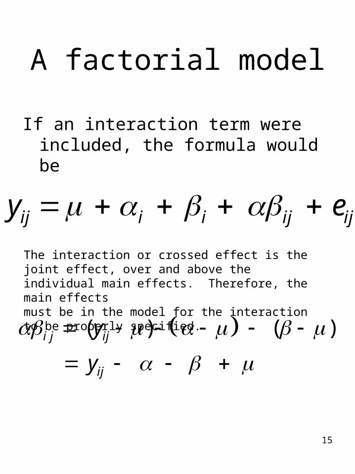
A factorial model

If an interaction term were included, the formula would be

ij i i ij ijy e The interaction or crossed effect is the joint effect, over and above the individual main effects. Therefore, the main effects must be in the model for the interaction to be properly specified.

( ) ( )i j ij

ij

y

y

16

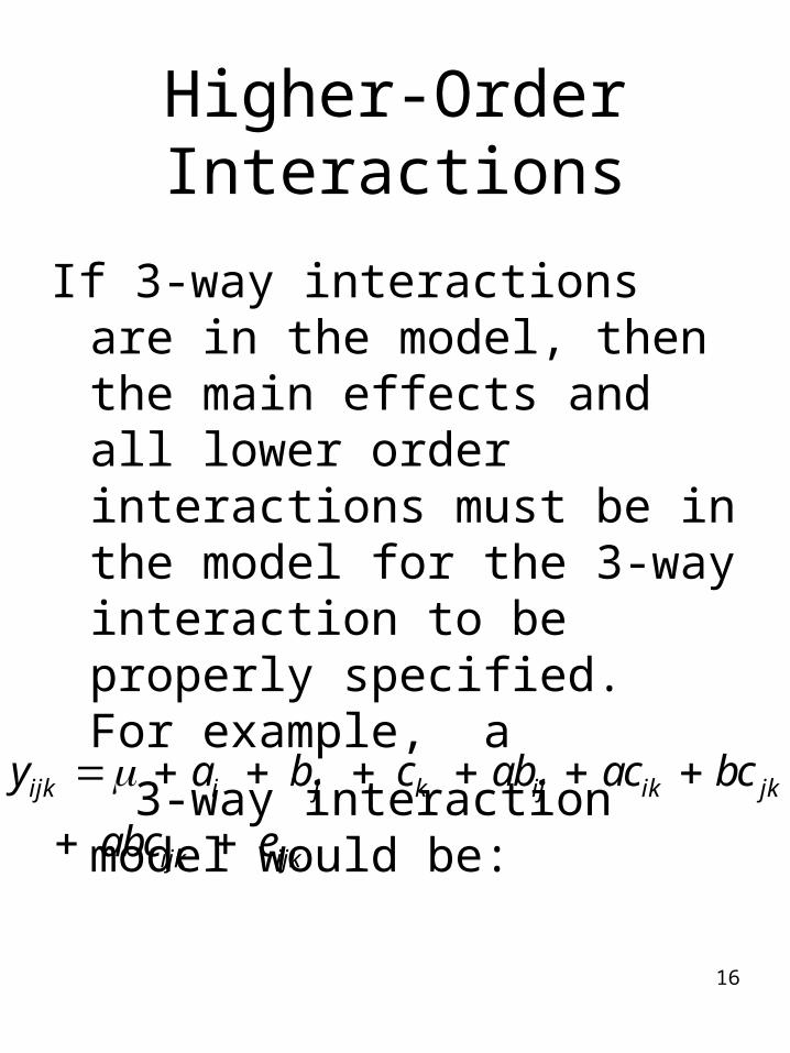
Higher-Order Interactions

If 3-way interactions are in the model, then the main effects and all lower order interactions must be in the model for the 3-way interaction to be properly specified. For example, a

3-way interaction model would be:

ijk i j k ij ik jk

ijk ijk

y a b c ab ac bc

abc e

17

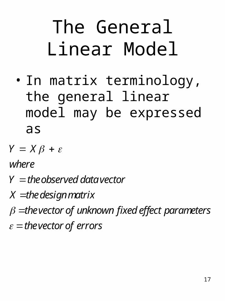
The General Linear Model

• In matrix terminology, the general linear model may be expressed as

Y XwhereY theobserved data vectorX the design matrix

thevector of unknown fixed effect parametersthevector of errors

18

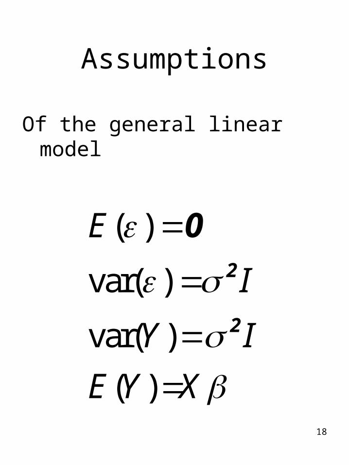
Assumptions

Of the general linear model

( )

var( )

var( )( )

E

I

Y IE Y X

2

2

0

19

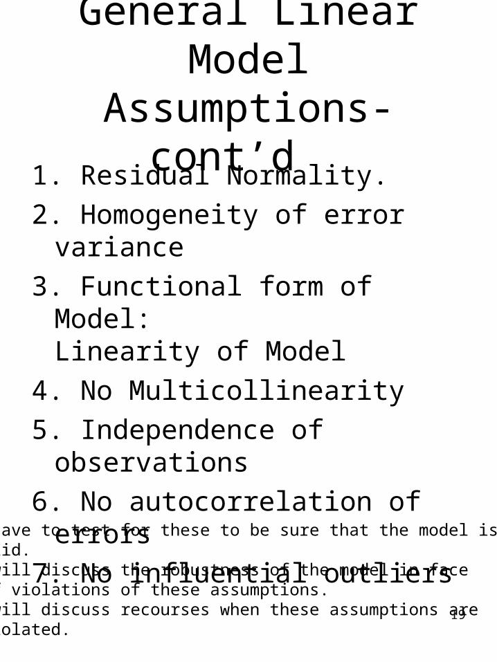
General Linear Model Assumptions-cont’d

1. Residual Normality.2. Homogeneity of error variance3. Functional form of Model:

Linearity of Model4. No Multicollinearity5. Independence of observations6. No autocorrelation of errors 7. No influential outliers

We have to test for these to be sure that the model is valid. We will discuss the robustness of the model in face of violations of these assumptions.We will discuss recourses when these assumptions are violated.

20

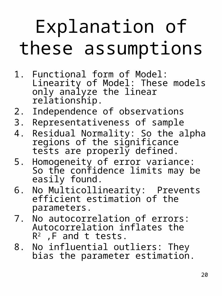
Explanation of these assumptions

1. Functional form of Model: Linearity of Model: These models only analyze the linear relationship.

2. Independence of observations3. Representativeness of sample4. Residual Normality: So the alpha

regions of the significance tests are properly defined.

5. Homogeneity of error variance: So the confidence limits may be easily found.

6. No Multicollinearity: Prevents efficient estimation of the parameters.

7. No autocorrelation of errors: Autocorrelation inflates the R2 ,F and t tests.

8. No influential outliers: They bias the parameter estimation.

21

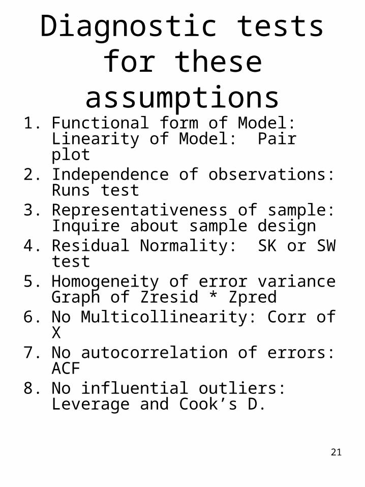
Diagnostic tests for these assumptions

1. Functional form of Model: Linearity of Model: Pair plot

2. Independence of observations: Runs test

3. Representativeness of sample: Inquire about sample design

4. Residual Normality: SK or SW test

5. Homogeneity of error variance Graph of Zresid * Zpred

6. No Multicollinearity: Corr of X7. No autocorrelation of errors: ACF8. No influential outliers: Leverage

and Cook’s D.

22

Testing for outliers

Frequencies analysis of stdres cksd.

Look for standardized residuals greater than 3.5 or less than – 3.5

• And look for Cook’s D.

23

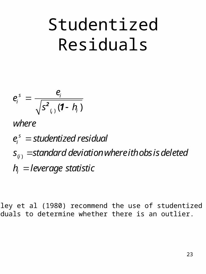
Studentized Residuals

( )

( )

( )i

s ii

i

si

i

i

ee

s h

where

e studentized residuals standard deviation whereithobs is deleted

h leverage statistic

2 1

Belsley et al (1980) recommend the use of studentizedResiduals to determine whether there is an outlier.

24

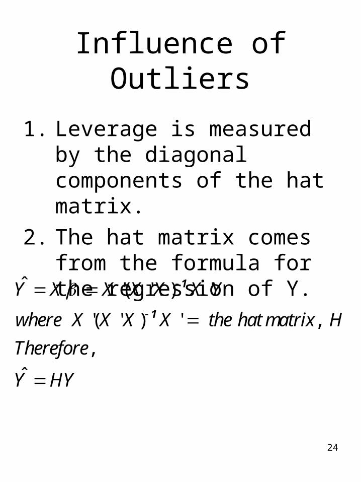
Influence of Outliers

1. Leverage is measured by the diagonal components of the hat matrix.

2. The hat matrix comes from the formula for the regression of Y.

ˆ '( ' ) '

'( ' ) ' ,,

ˆ

Y X X X X X Y

where X X X X the hat matrix HTherefore

Y HY

1

1

25

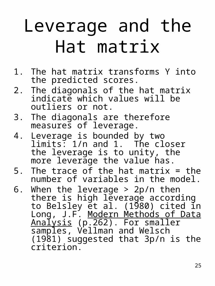
Leverage and the Hat matrix

1. The hat matrix transforms Y into the predicted scores.

2. The diagonals of the hat matrix indicate which values will be outliers or not.

3. The diagonals are therefore measures of leverage.

4. Leverage is bounded by two limits: 1/n and 1. The closer the leverage is to unity, the more leverage the value has.

5. The trace of the hat matrix = the number of variables in the model.

6. When the leverage > 2p/n then there is high leverage according to Belsley et al. (1980) cited in Long, J.F. Modern Methods of Data Analysis (p.262). For smaller samples, Vellman and Welsch (1981) suggested that 3p/n is the criterion.

26

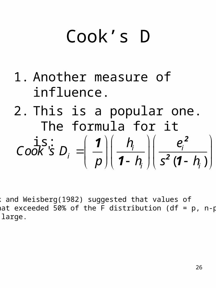
Cook’s D

1. Another measure of influence.

2. This is a popular one. The formula for it is:

'( )

i ii

i i

h eCook s Dp h s h

2

2

11 1

Cook and Weisberg(1982) suggested that values of D that exceeded 50% of the F distribution (df = p, n-p)are large.

27

Cook’s D in SPSS

Finding the influential outliersSelect those observations for which

cksd > (4*p)/n Belsley suggests 4/(n-p-1) as a

cutoffIf cksd > (4*p)/(n-p-1);

28

What to do with outliers

1. Check coding to spot typos2. Correct typos3. If observational outlier is correct,

examine the dffits option to see the influence on the fitting statistics.

4. This will show the standardized influence of the observation on the fit. If the influence of the outlier is bad, then consider removal or replacement of it with imputation.

29

Decomposition of the Sums of Squares

1. Mean deviations are computed when means are subtracted from individual scores.

1. This is done for the total, the group mean, and the error terms.

2. Mean deviations are squared and these are called sums of squares

3. Variances are computed by dividing the Sums of Squares by their degrees of freedom.

4. The total Variance = Model Variance + error variance

30

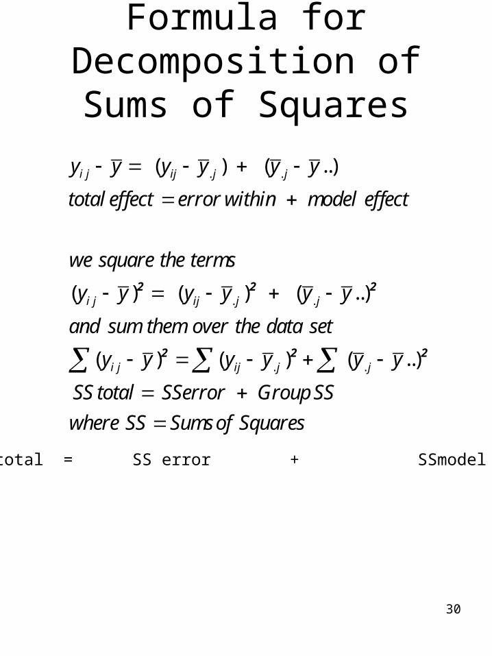
Formula for Decomposition of Sums of Squares

SS total = SS error + SSmodel

. .

. .

. .

( ) ( ..)

( ) ( ) ( ..)

( ) ( ) ( ..)

i j ij j j

i j ij j j

i j ij j j

y y y y y y

total effect error within model effect

we square the terms

y y y y y y

and sum them over the data set

y y y y y y

SS total SSerror Group SSwhere SS Sums of

2 2 2

2 2 2

Squares

31

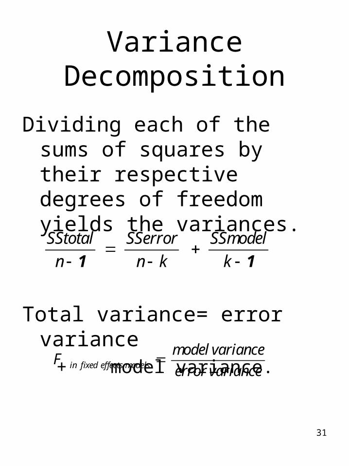
Variance Decomposition

Dividing each of the sums of squares by their respective degrees of freedom yields the variances.

Total variance= error variance + model variance.

in fixed effects modelsmodel varianceFerror variance

SStotal SSerror SSmodeln n k k

1 1

32

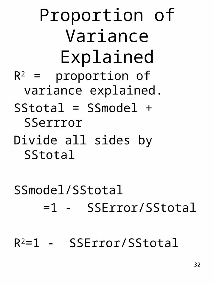
Proportion of Variance Explained

R2 = proportion of variance explained.

SStotal = SSmodel + SSerrrorDivide all sides by SStotal

SSmodel/SStotal =1 - SSError/SStotal

R2=1 - SSError/SStotal

33

The Omnibus F test

The omnibus F test is a test that all of the means of the levels of the main effects and as well as any interactions specified are not significantly different from one another.

Suppose the model is a one way anova on breakingpressure of bonds of different metals.

Suppose there are three metals: nickel, iron, andCopper.

H0: Mean(Nickel)= mean (Iron) = mean(Copper)Ha: Mean(Nickel) ne Mean(Iron) or Mean(Nickel) ne Mean(Copper) or Mean(Iron) ne Mean(Copper)

34

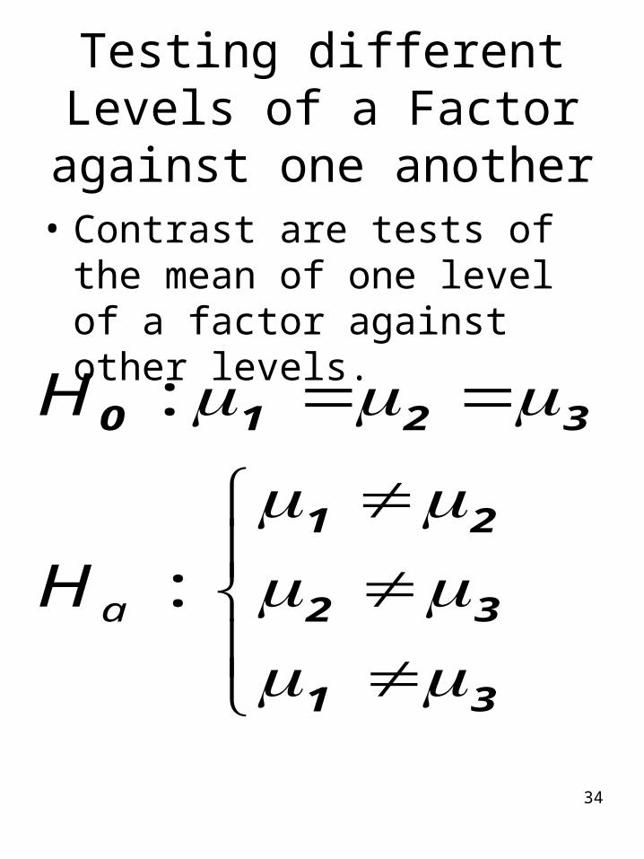
Testing different Levels of a Factor against one

another• Contrast are tests of the mean

of one level of a factor against other levels.

:

:a

H

H

0 1 2 3

1 2

2 3

1 3

35

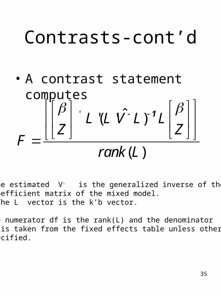
Contrasts-cont’d

• A contrast statement computes

' ˆ'( ' )

( )

L L V L LZ Z

Frank L

1

The estimated V- is the generalized inverse of the coefficient matrix of the mixed model. The L vector is the k’b vector.

The numerator df is the rank(L) and the denominatordf is taken from the fixed effects table unless otherwisespecified.

36

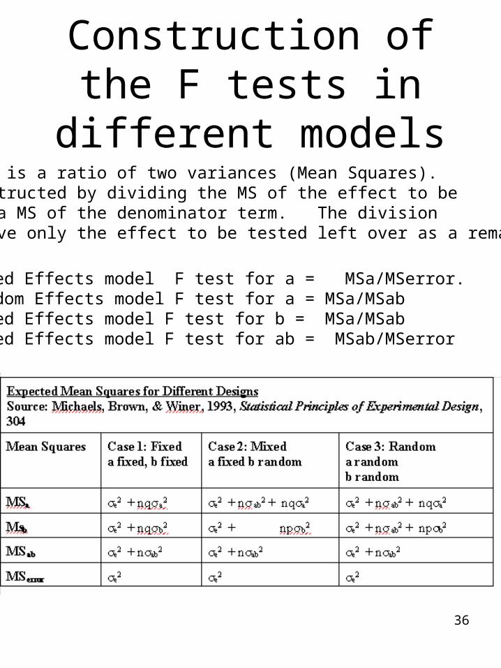
Construction of the F tests in different models

The F test is a ratio of two variances (Mean Squares).It is constructed by dividing the MS of the effect to betested by a MS of the denominator term. The divisionshould leave only the effect to be tested left over as a remainder.

A Fixed Effects model F test for a = MSa/MSerror.A Random Effects model F test for a = MSa/MSabA Mixed Effects model F test for b = MSa/MSabA Mixed Effects model F test for ab = MSab/MSerror

37

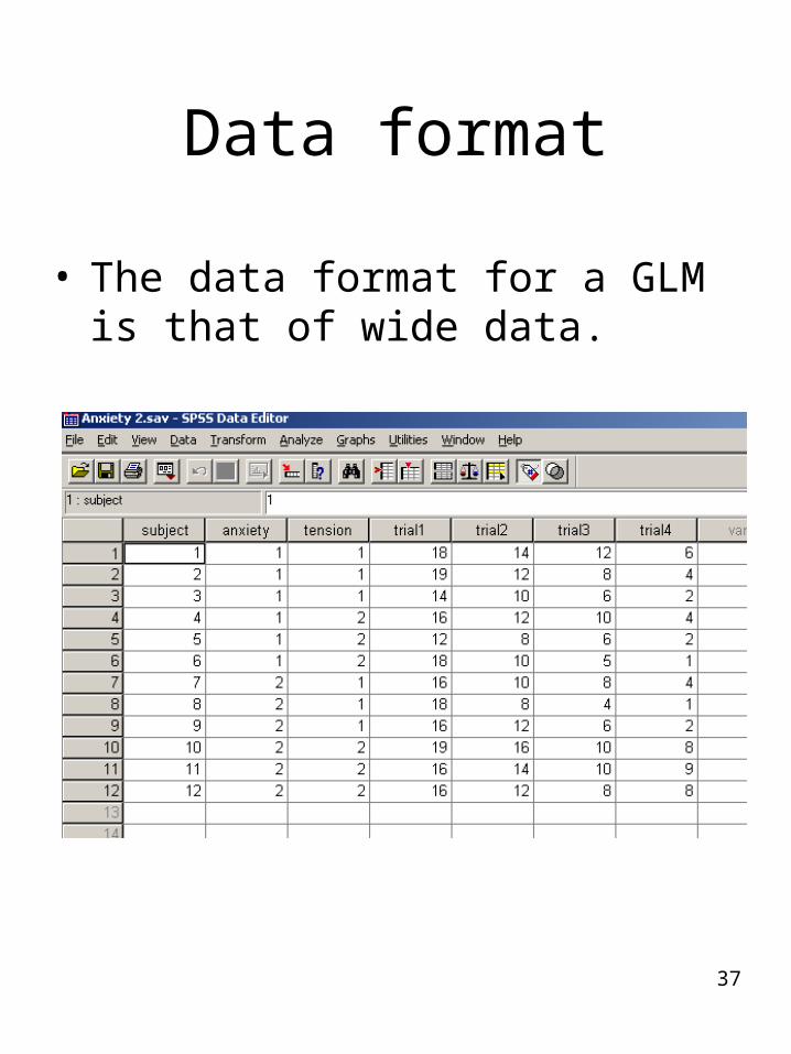
Data format

• The data format for a GLM is that of wide data.

38

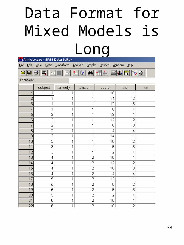
Data Format for Mixed Models is Long

39

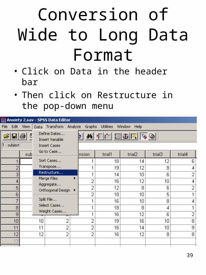
Conversion of Wide to Long Data Format

• Click on Data in the header bar• Then click on Restructure in the

pop-down menu

40

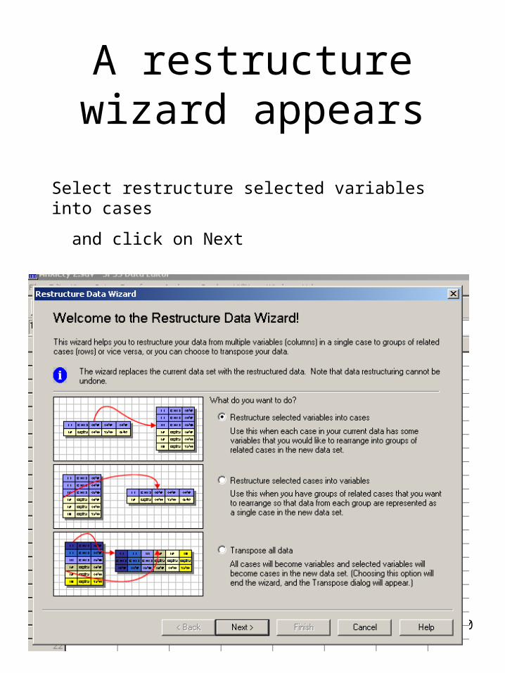
A restructure wizard appears

Select restructure selected variables into cases

and click on Next

41

A Variables to Cases: Number of Variable Groups dialog box appears.

We select one and click on next.

42

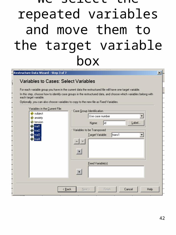
We select the repeated variables and move them to the target variable box

43

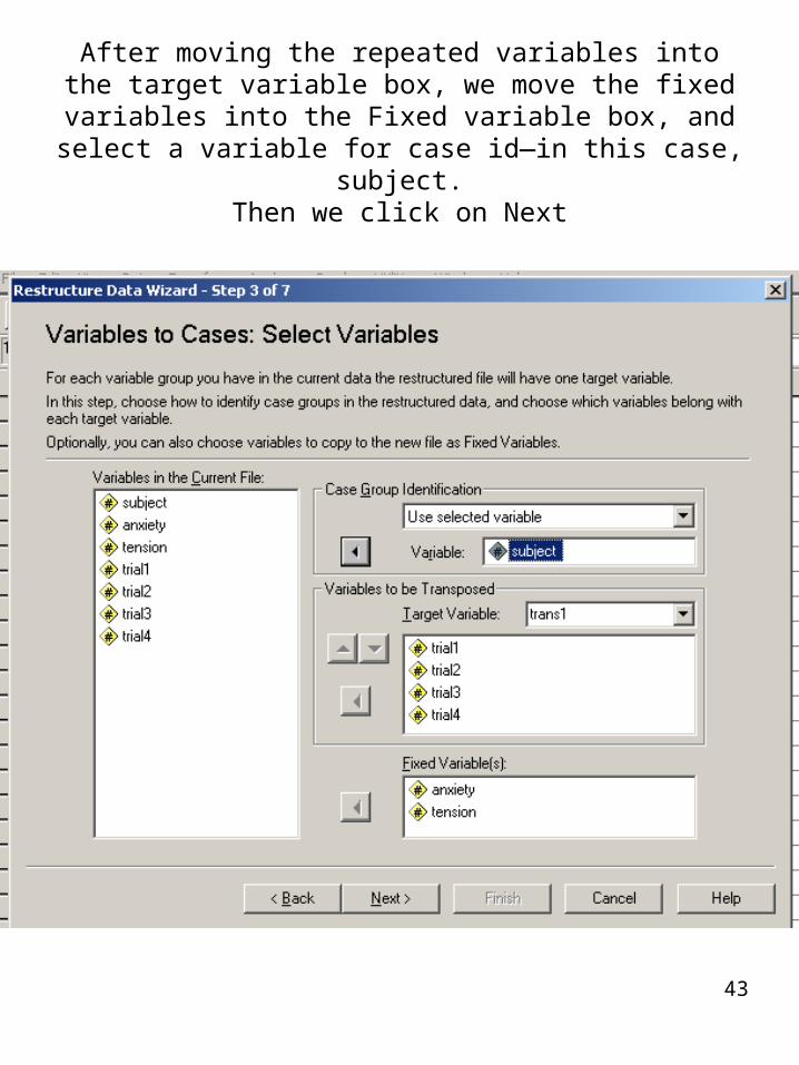
After moving the repeated variables into the target variable box, we move the fixed variables into the Fixed variable

box, and select a variable for case id—in this case, subject.Then we click on Next

44

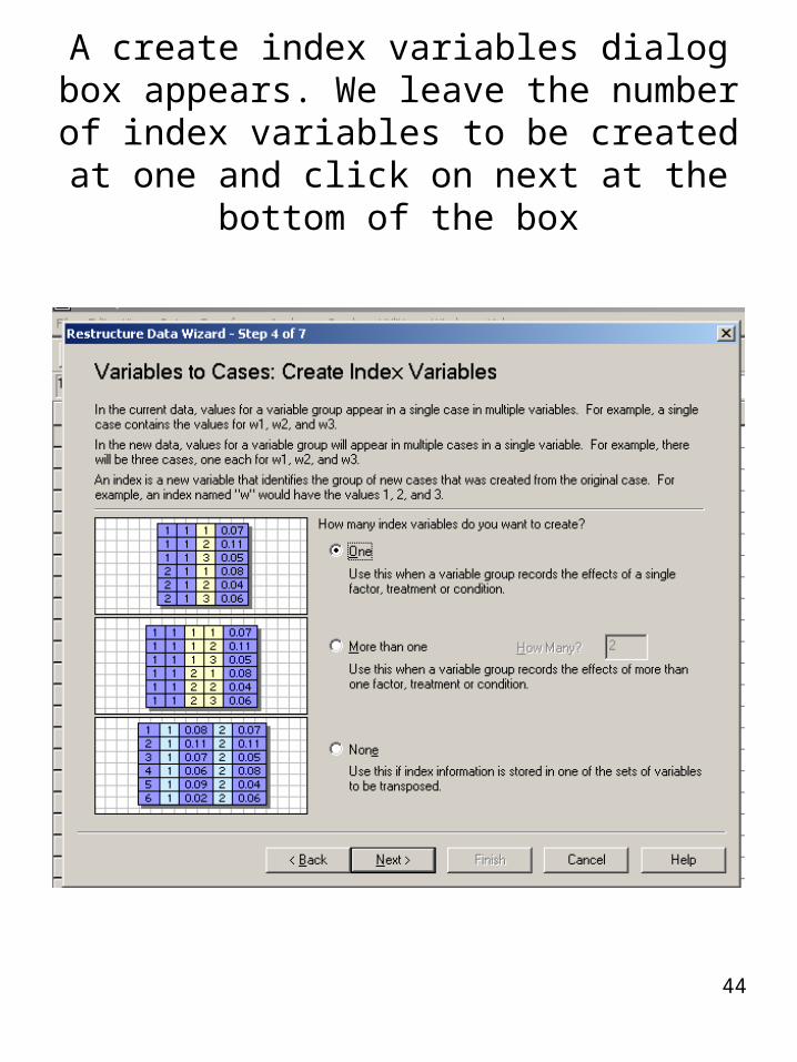
A create index variables dialog box appears. We leave the number of index

variables to be created at one and click on next at the bottom of the box

45

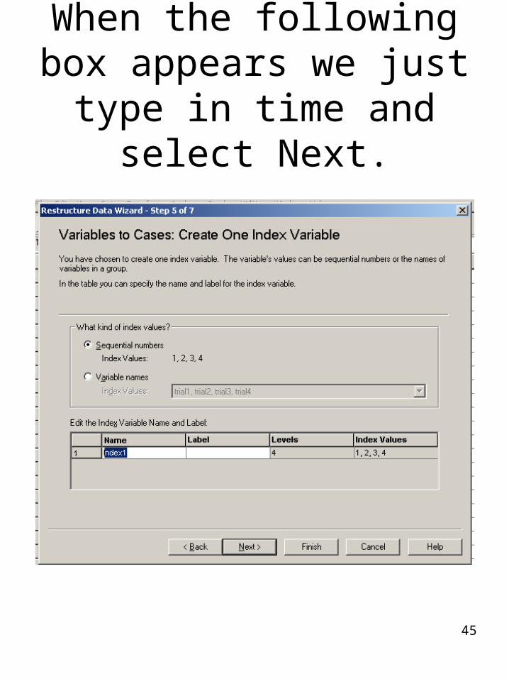
When the following box appears we just type in time and select Next.

46

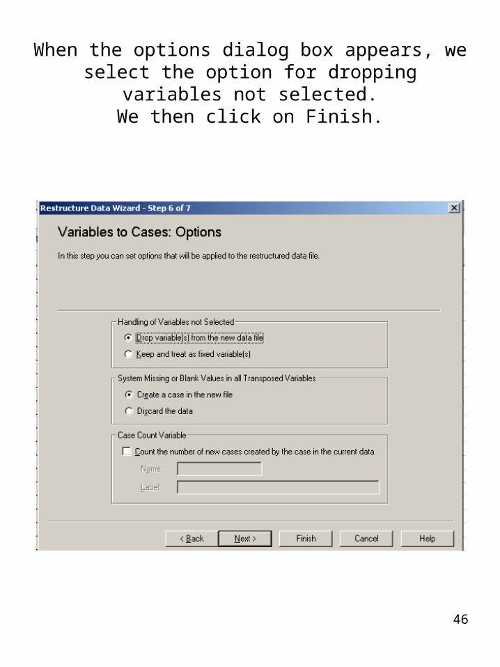
When the options dialog box appears, we select the option for dropping variables not selected.

We then click on Finish.

47

We thus obtain our data in long format

48

The Mixed Model

The Mixed Model uses long data format. It includes fixed and random effects.

It can be used to model merely fixed or random effects, by zeroing out the other parameter vector.

The F tests for the fixed, random, and mixed models differ.

Because the Mixed Model has the parameter vector for both of these and can estimate the error covariance matrix for each, it can provide the correct standard errors for either the

fixed or random effects.

49

The Mixed Model

'

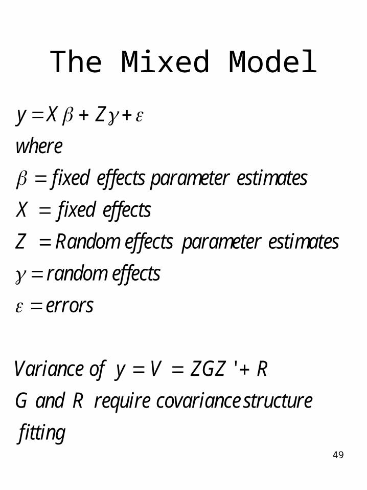
y X Zwhere

fixed effects parameter estimatesX fixed effectsZ Random effects parameter estimates

random effectserrors

Variance of y V ZGZ RG and R require covariance structurefitting

50

Mixed Model Theory-cont’d

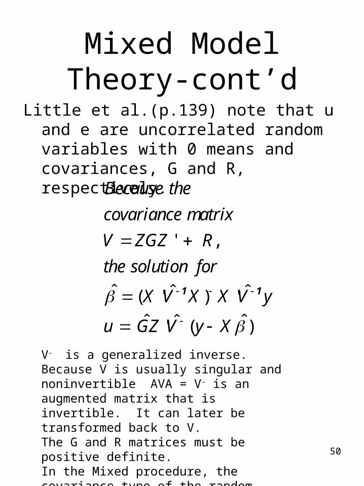
Little et al.(p.139) note that u and e are uncorrelated random variables with 0 means and covariances, G and R, respectively.

' ,

ˆ ˆ ˆ( ' ) 'ˆ ˆˆ' ( )

Because thecovariance matrixV ZGZ Rthe solution for

X V X X V y

u GZ V y X

1 1

V- is a generalized inverse. Because V is usually singular and noninvertible AVA = V- is an augmented matrix that is invertible. It can later be transformed back to V.The G and R matrices must be positive definite.In the Mixed procedure, the covariance type of the random (generalized) effects defines the structure of G and a repeated covariance type defines structure of R.

51

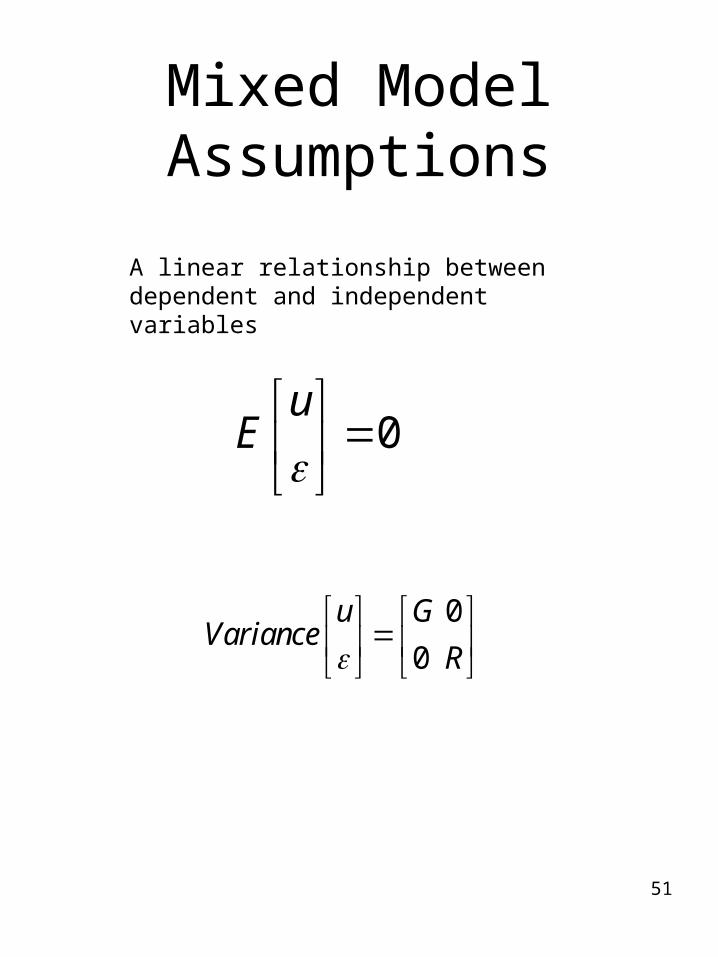
Mixed Model Assumptions

0u

E

00

u GVariance

R

A linear relationship between dependent and independent variables

52

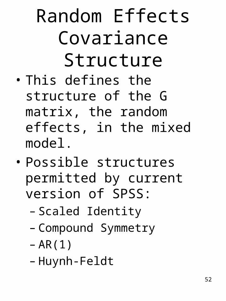
Random Effects Covariance Structure

• This defines the structure of the G matrix, the random effects, in the mixed model.

• Possible structures permitted by current version of SPSS:– Scaled Identity– Compound Symmetry– AR(1)– Huynh-Feldt

53

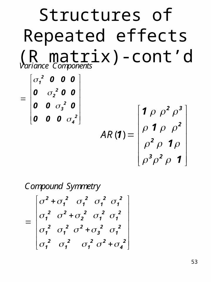
Structures of Repeated effects (R matrix)-cont’d

Variance Components

21

22

23

24

0 0 0

0 0 0

0 0 0

0 0 0

Compound Symmetry

2 2 2 2 21 1 1 1

2 2 2 2 21 2 1 1

2 2 2 2 21 1 3 1

2 2 2 2 21 1 1 4

( )AR

2 3

2

2

3 2

1

11

1

1

54

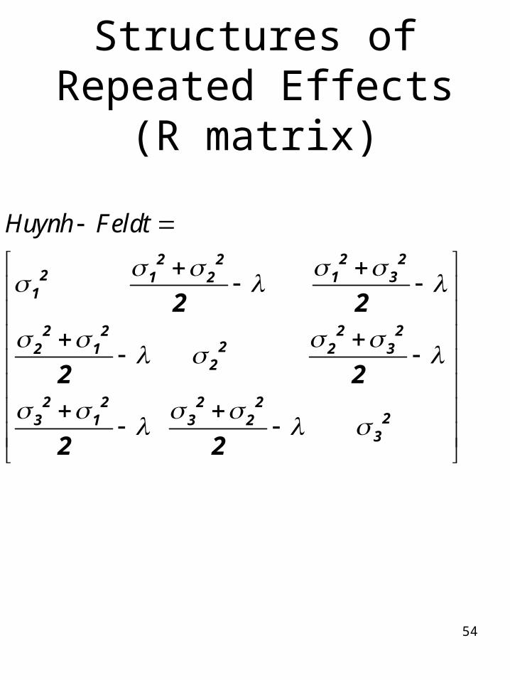
Structures of Repeated Effects (R matrix)

Huynh Feldt

2 22 22 1 31 21

2 22 22 2 32 12

2 2 2 223 1 3 23

2 2

2 2

2 2

55

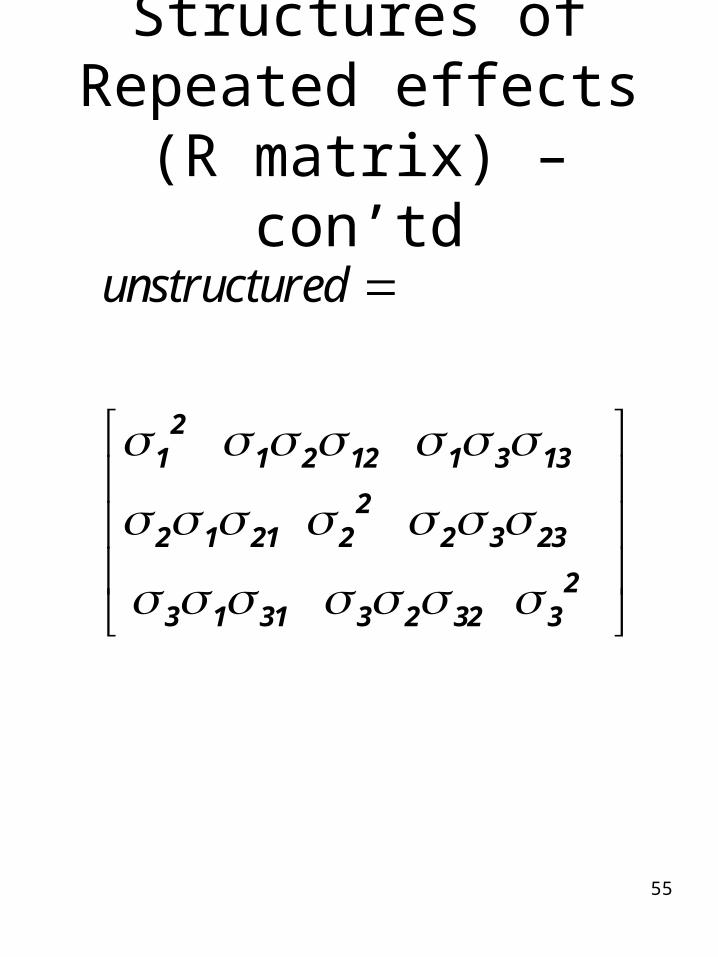
Structures of Repeated effects (R matrix) –con’td

unstructured

21 1 2 12 1 3 13

22 1 21 2 2 3 23

23 1 31 3 2 32 3

56

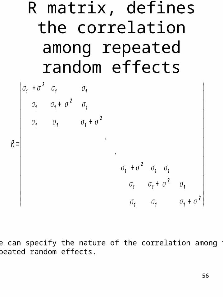
R matrix, defines the correlation among

repeated random effects

..

R

21 1 1

21 1 1

21 1 1

21 1 1

21 1 1

21 1 1

One can specify the nature of the correlation among therepeated random effects.

57

GLM Mixed Model

The General Linear Model is a special case of theMixed Model with Z = 0 (which means thatZu disappears from the model) and 2R I

58

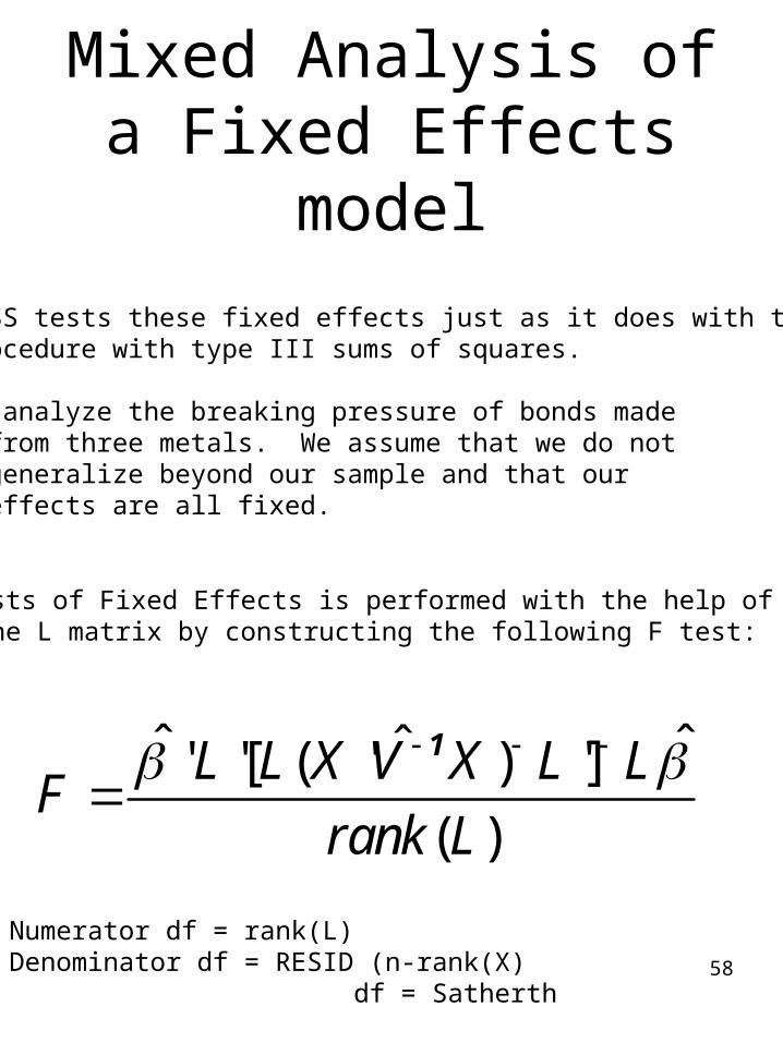
Mixed Analysis of a Fixed Effects model

SPSS tests these fixed effects just as it does with the GLMProcedure with type III sums of squares.

We analyze the breaking pressure of bonds made from three metals. We assume that we do not generalize beyond our sample and that our effects are all fixed.

Tests of Fixed Effects is performed with the help of the L matrix by constructing the following F test:

ˆ ˆˆ' '[ ( ' ) ']( )

L L X V X L LFrank L

1

Numerator df = rank(L)Denominator df = RESID (n-rank(X) df = Satherth

59

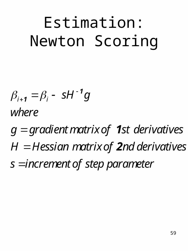
Estimation: Newton Scoring

i i sH gwhereg gradient matrix of st derivativesH Hessian matrix of nd derivativess increment of step parameter

11

12

60

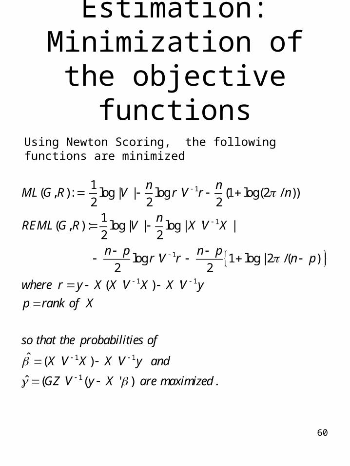
Estimation: Minimization of the objective functions

1

1

1

1 1

1 1

1( , ): log | | log ' (1 log(2 / ))2 2 2

1( , ) : log | | log | ' |2 2

log ' 1 log | 2 /( ) |2 2

( ' ) '

ˆ ( ' ) 'ˆ ( '

n nML G R V r V r n

nREML G R V X V X

n p n pr V r n p

where r y X X V X X V yp rank of X

so that the probabilities of

X V X X V y and

GZ V

1( ' ) .y X are maximized

Using Newton Scoring, the following functions are minimized

61

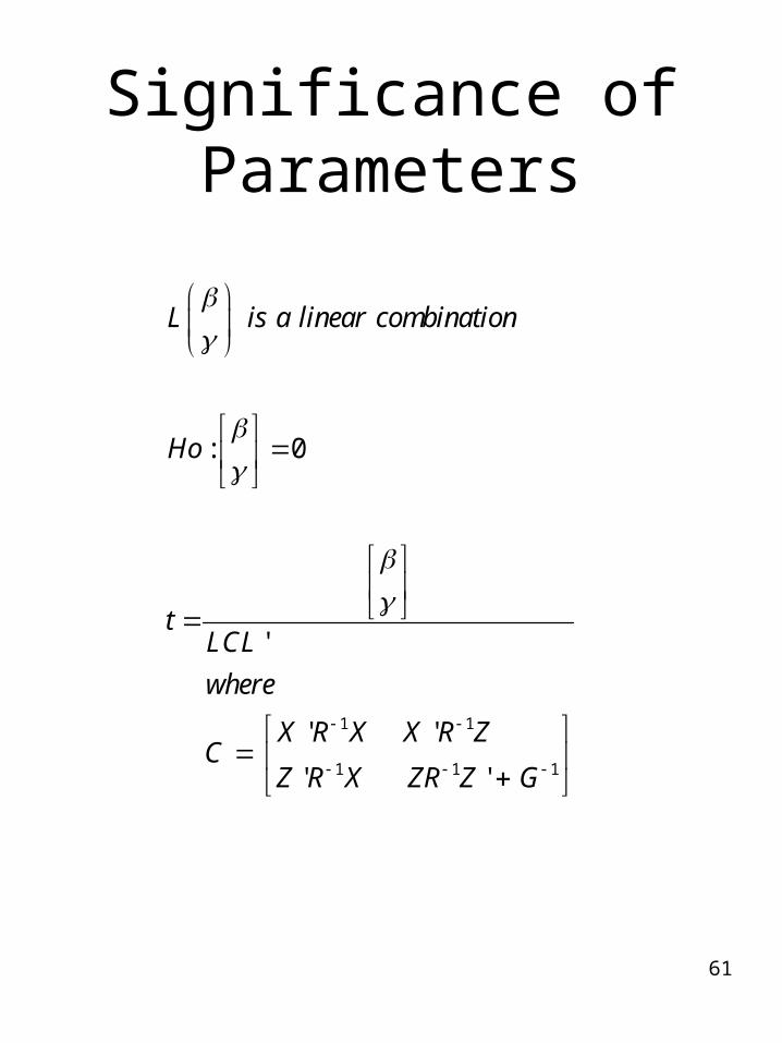
Significance of Parameters

1 1

1 1 1

: 0

'

' '

' '

L is a linear combination

Ho

tLCLwhere

X R X X R ZC

Z R X ZR Z G

62

Test one covariance structure against the other

with the IC• The rule of thumb is smaller is

better• -2LL• AIC Akaike• AICC Hurvich and Tsay• BIC Bayesian Info Criterion• Bozdogan’s CAIC

63

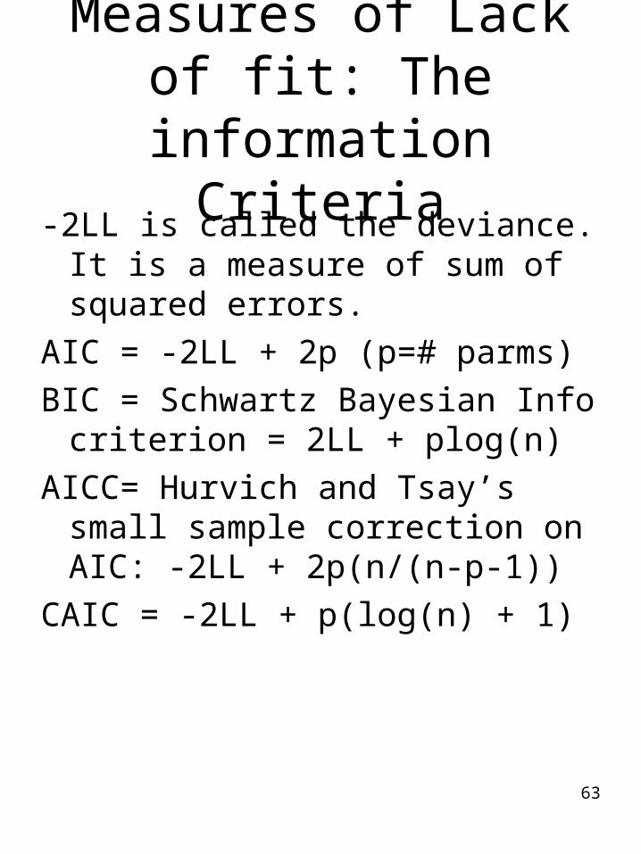
Measures of Lack of fit: The information Criteria

-2LL is called the deviance. It is a measure of sum of squared errors.

AIC = -2LL + 2p (p=# parms)BIC = Schwartz Bayesian Info

criterion = 2LL + plog(n)AICC= Hurvich and Tsay’s small

sample correction on AIC: -2LL + 2p(n/(n-p-1))

CAIC = -2LL + p(log(n) + 1)

64

Procedures for Fitting the Mixed Model

• One can use the LR test or the lesser of the information criteria. The smaller the information criterion, the better the model happens to be.

• We try to go from a larger to a smaller information criterion when we fit the model.

65

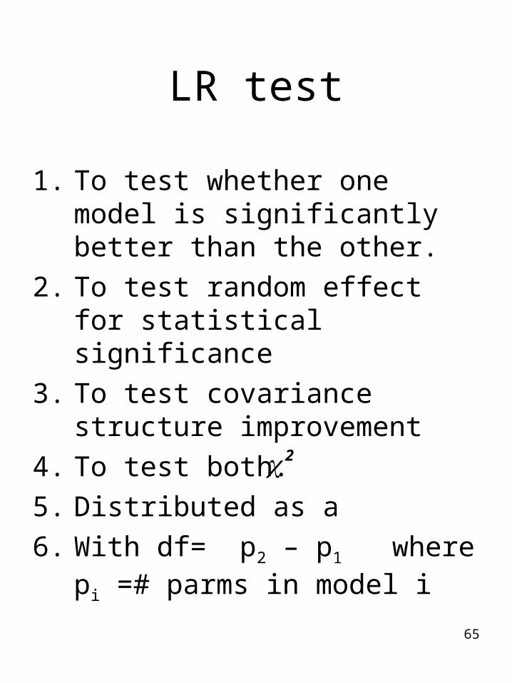
LR test

1. To test whether one model is significantly better than the other.

2. To test random effect for statistical significance

3. To test covariance structure improvement

4. To test both.5. Distributed as a 6. With df= p2 – p1 where pi =#

parms in model i

2

66

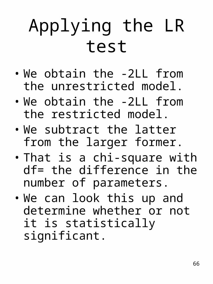
Applying the LR test

• We obtain the -2LL from the unrestricted model.

• We obtain the -2LL from the restricted model.

• We subtract the latter from the larger former.

• That is a chi-square with df= the difference in the number of parameters.

• We can look this up and determine whether or not it is statistically significant.

67

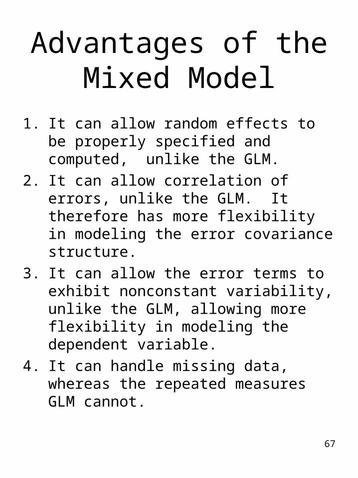
Advantages of the Mixed Model

1. It can allow random effects to be properly specified and computed, unlike the GLM.

2. It can allow correlation of errors, unlike the GLM. It therefore has more flexibility in modeling the error covariance structure.

3. It can allow the error terms to exhibit nonconstant variability, unlike the GLM, allowing more flexibility in modeling the dependent variable.

4. It can handle missing data, whereas the repeated measures GLM cannot.

68

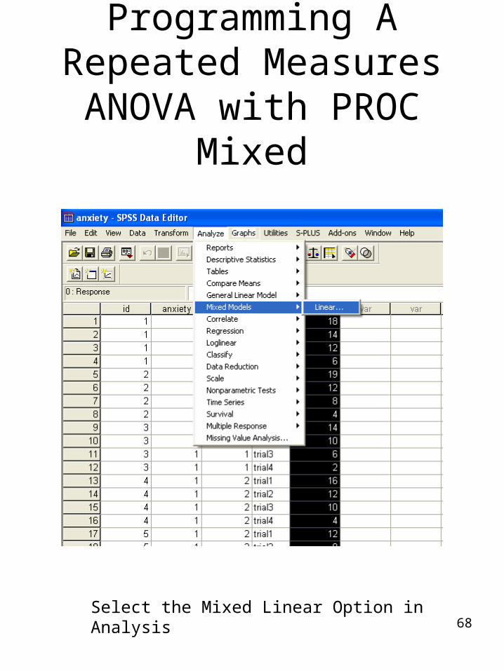
Programming A Repeated Measures ANOVA with

PROC Mixed

Select the Mixed Linear Option in Analysis

69

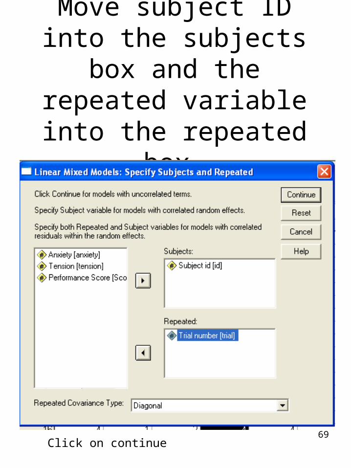
Move subject ID into the subjects box and the

repeated variable into the repeated box.

Click on continue

70

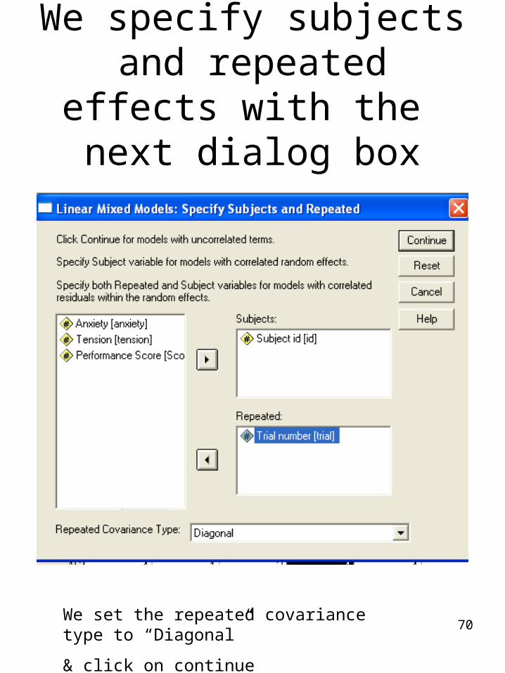
We specify subjects and repeated effects with the

next dialog box

We set the repeated covariance type to “Diagonal”

& click on continue

71

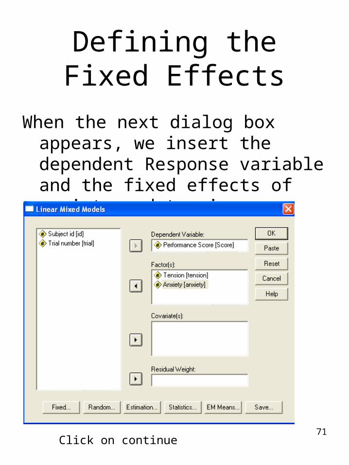
Defining the Fixed Effects

When the next dialog box appears, we insert the dependent Response variable and the fixed effects of anxiety and tension

Click on continue

72

We select the Fixed effects to be tested

73

Move them into the model box, selecting main effects, and type III

sum of squares

Click on continue

74

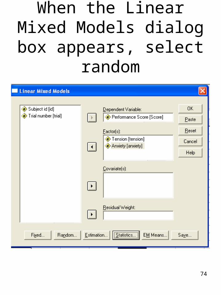
When the Linear Mixed Models dialog box

appears, select random

75

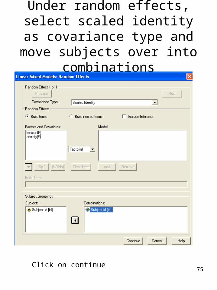
Under random effects, select scaled identity as covariance

type and move subjects over into combinations

Click on continue

76

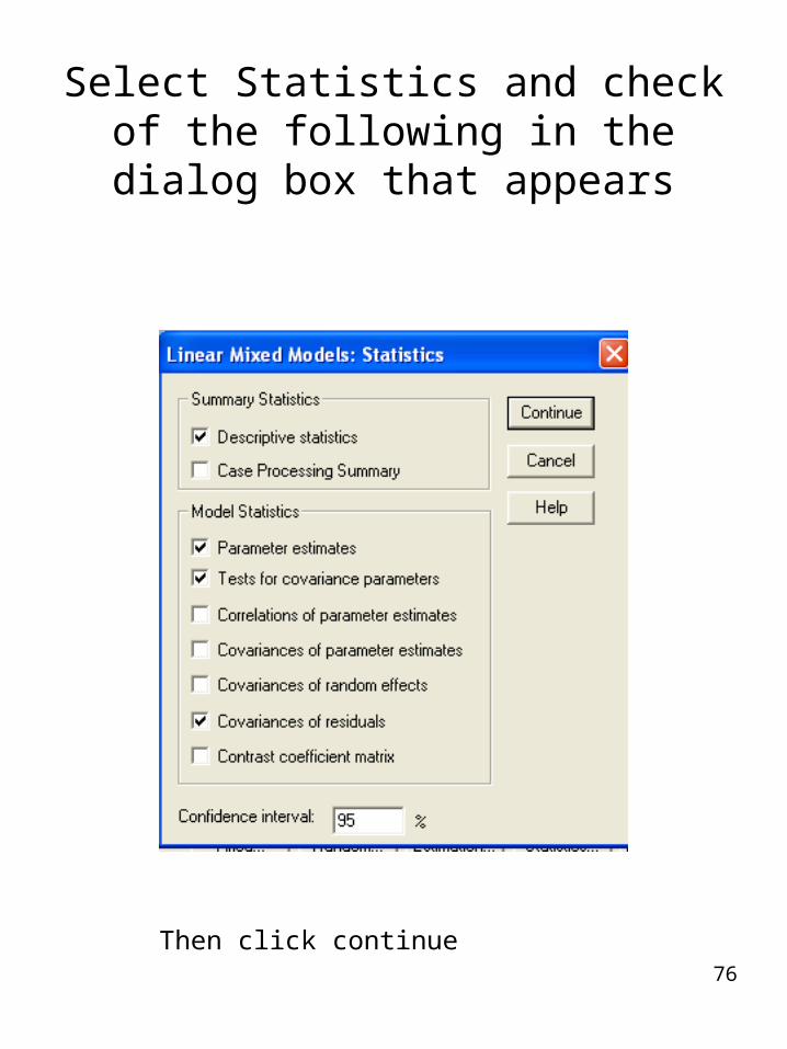
Select Statistics and check of the following in the dialog box that

appears

Then click continue

77

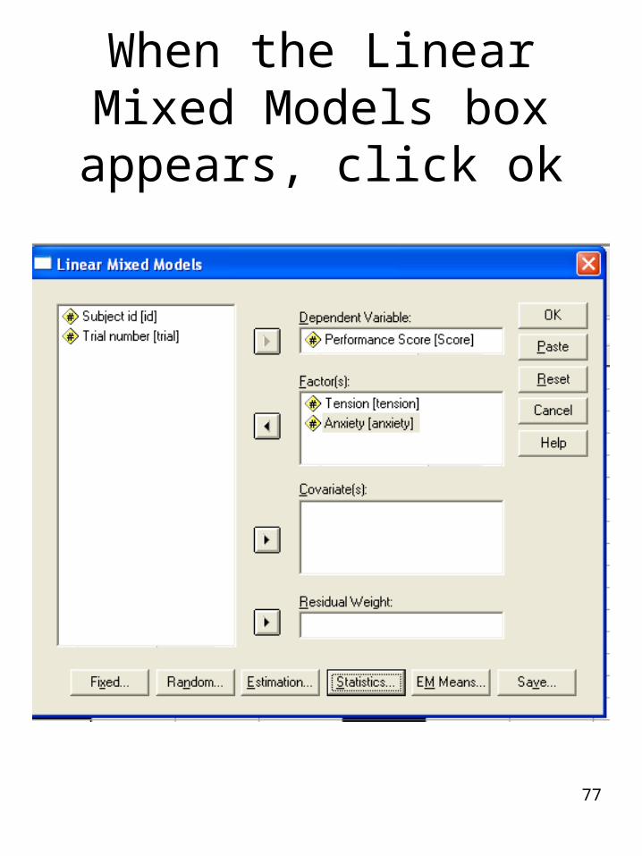
When the Linear Mixed Models box appears, click

ok

78

You will get your tests

79

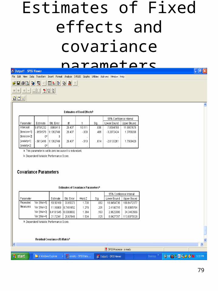
Estimates of Fixed effects and covariance

parameters

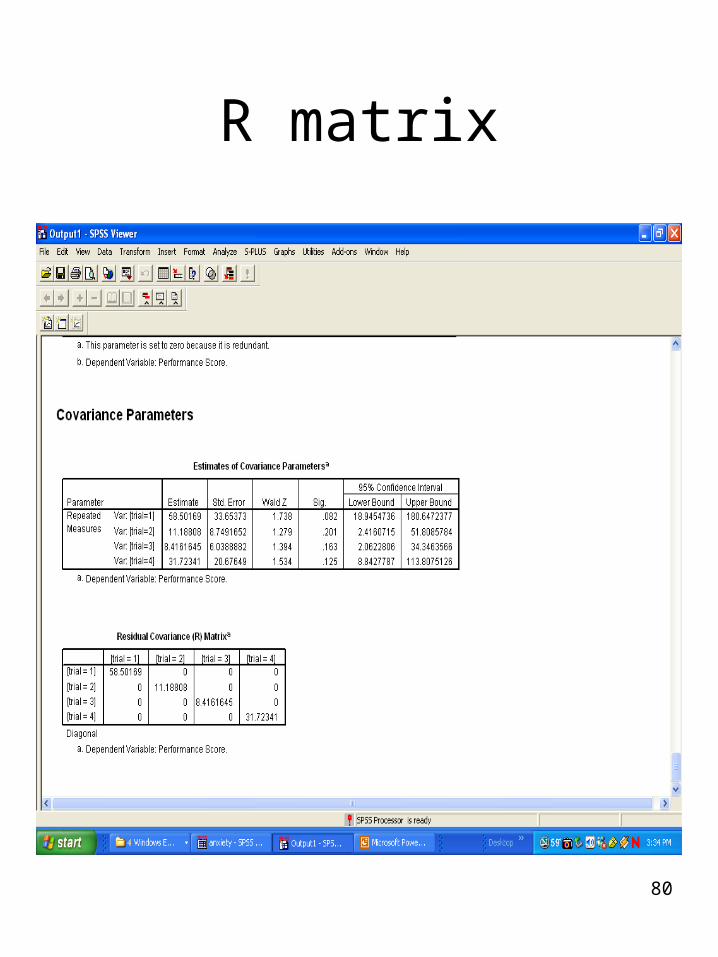
80

R matrix

81

Rerun the model with different nested covariance structures and compare the

information criteria

The lower the information criterion, the better fit the nested model has. Caveat: If the models are not nested, they cannot be compared with the information criteria.

82

GLM vs. Mixed

GLM has means lsmeans sstype 1,2,3,4 estimates using OLS or WLS one has to program the correct F tests for random

effects. losses cases with missing values.Mixed has lsmeans sstypes 1 and 3 estimates using maximum likelihood, general methods

of moments, or restricted maximum likelihood ML MIVQUE0 REML gives correct std errors and confidence intervals for

random effects Automatically provides correct standard errors for

analysis. Can handle missing values