Anova

ANOVA An Introduction to Experimental

Design and Analysis of Variance Analysis of Variance and the Completely Randomized Design

Multiple Comparison Procedures

Statistical studies can be classified as being either experimental or observational.

In an experimental study, one or more factors are controlled so that data can be obtained about how the factors influence the variables of interest. In an observational study, no attempt is made to control the factors.

Cause-and-effect relationships are easier to establish in experimental studies than in observational studies.

An Introduction to Experimental Designand Analysis of Variance

Analysis of variance (ANOVA) can be used to analyze the data obtained from experimental or observational studies.

An Introduction to Experimental Designand Analysis of Variance A factor is a variable that the experimenter

has selected for investigation. A treatment is a level of a factor. Experimental units are the objects of interest

in the experiment. A completely randomized design is an

experimental design in which the treatments are randomly assigned to the experimental units.

Analysis of Variance: A Conceptual Overview

Analysis of Variance (ANOVA) can be used to test for the equality of three or more population means. Analysis of Variance (ANOVA) can be used to test for the equality of three or more population means.

Data obtained from observational or experimental studies can be used for the analysis. Data obtained from observational or experimental studies can be used for the analysis.

We want to use the sample results to test the following hypotheses: We want to use the sample results to test the following hypotheses:

H0: 1=2=3=. . . = k

Ha: Not all population means are equal

H0: 1=2=3=. . . = k


If H0 is rejected, we cannot conclude that all population means are different.

If H0 is rejected, we cannot conclude that all population means are different.

Rejecting H0 means that at least two population means have different values.

Rejecting H0 means that at least two population means have different values.


For each population, the response (dependent) variable is normally distributed. For each population, the response (dependent) variable is normally distributed.

The variance of the response variable, denoted 2, is the same for all of the populations. The variance of the response variable, denoted 2, is the same for all of the populations.

The observations must be independent. The observations must be independent.

Assumptions for Analysis of Variance


Sampling Distribution of Given H0 is Truex

1x 3x2x

Sample means are close together because there is only one sampling distribution when H0 is true.

22x n


Sampling Distribution of Given H0 is Falsex

33 1x 2x3x 11 22

Sample means come fromdifferent sampling distributionsand are not as close together when H0 is false.


Analysis of Variance andthe Completely Randomized Design

Between-Treatments Estimate of Population Variance Within-Treatments Estimate of Population Variance Comparing the Variance Estimates: The F Test ANOVA Table

2

1

( )

MSTR1

k

j jj

n x x

k

Between-Treatments Estimateof Population Variance s 2

Denominator is thedegrees of freedomassociated with SSTR

Numerator is calledthe sum of squares dueto treatments (SSTR)

The estimate of 2 based on the variation of the

sample means is called the mean square due to

treatments and is denoted by MSTR.

The estimate of 2 based on the variation of the sample observations within each sample is called the mean square error and is denoted by MSE.

Within-Treatments Estimateof Population Variance s 2

Denominator is thedegrees of freedomassociated with SSE

Numerator is calledthe sum of squaresdue to error (SSE)

MSE

( )n s

n k

j jj

k

T

1 2

1MSE

( )n s

n k

j jj

k

T

1 2

1

Comparing the Variance Estimates: The F Test

If the null hypothesis is true and the ANOVA assumptions are valid, the sampling distribution of MSTR/MSE is an F distribution with MSTR d.f. equal to k - 1 and MSE d.f. equal to nT - k.

If the means of the k populations are not equal, the value of MSTR/MSE will be inflated because MSTR overestimates 2. Hence, we will reject H0 if the resulting value of MSTR/MSE appears to be too large to have been selected at random from the appropriate F distribution.

Sampling Distribution of MSTR/MSE

Do Not Reject H0Do Not Reject H0

Reject H0Reject H0

MSTR/MSEMSTR/MSE

Critical ValueCritical ValueFF

Sampling Distributionof MSTR/MSE

a

Comparing the Variance Estimates: The F Test

MSTRSSTR

-

k 1MSTR

SSTR-

k 1

MSESSE

-

n kT

MSESSE

-

n kT

MSTRMSE

MSTRMSE

Source ofVariation

Sum ofSquares

Degrees ofFreedom

MeanSquare F

Treatments

Error

Total

k - 1

nT - 1

SSTR

SSE

SST

nT - k

SST is partitionedinto SSTR and SSE.

SST’s degrees of freedom(d.f.) are partitioned intoSSTR’s d.f. and SSE’s d.f.

ANOVA Tablefor a Completely Randomized Design

p-Value

SST divided by its degrees of freedom nT – 1 is the overall sample variance that would be obtained if we treated the entire set of observations as one data set.

SST divided by its degrees of freedom nT – 1 is the overall sample variance that would be obtained if we treated the entire set of observations as one data set.

With the entire data set as one sample, the formula for computing the total sum of squares, SST, is: With the entire data set as one sample, the formula for computing the total sum of squares, SST, is:

2

1 1

SST ( ) SSTR SSEjnk

ijj i

x x


ANOVA can be viewed as the process of partitioning the total sum of squares and the degrees of freedom into their corresponding sources: treatments and error.

ANOVA can be viewed as the process of partitioning the total sum of squares and the degrees of freedom into their corresponding sources: treatments and error.

Dividing the sum of squares by the appropriate degrees of freedom provides the variance estimates and the F value used to test the hypothesis of equal population means.

Dividing the sum of squares by the appropriate degrees of freedom provides the variance estimates and the F value used to test the hypothesis of equal population means.


Test for the Equality of k Population Means

F = MSTR/MSE

H0: 1=2=3=. . . = k


Hypotheses

Test Statistic

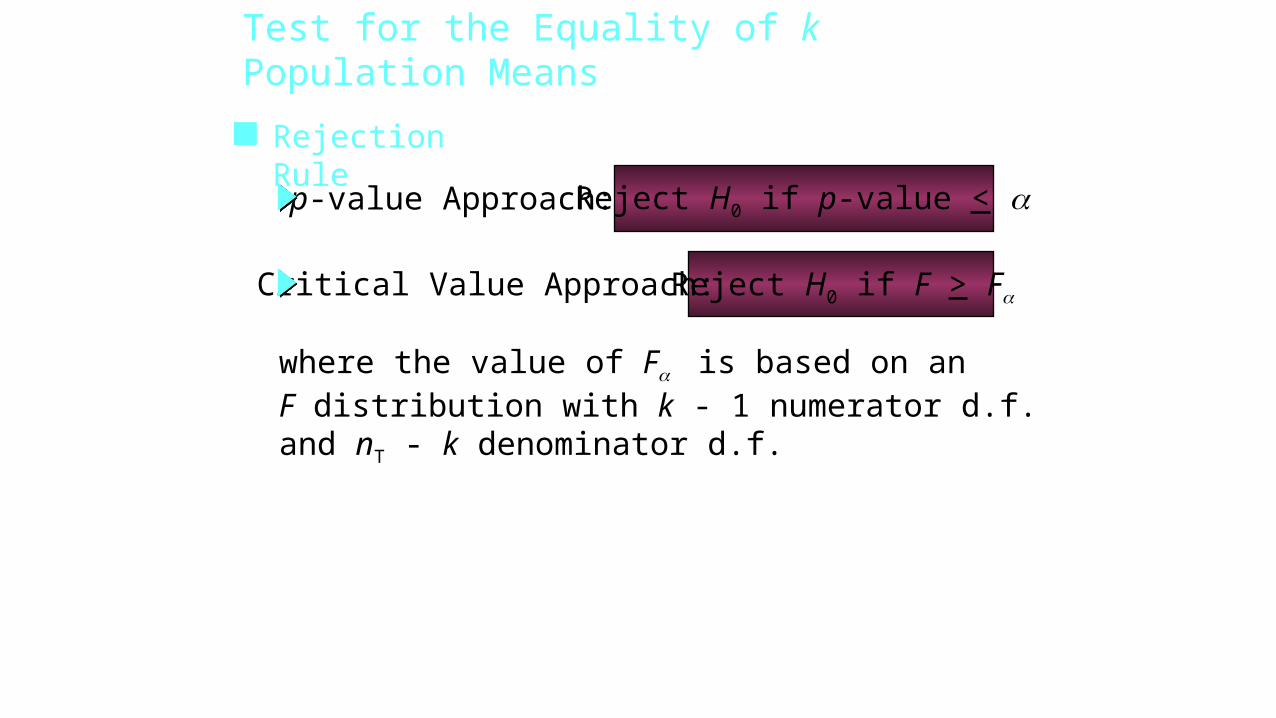
Test for the Equality of k Population Means

Rejection Rule

where the value of F is based on anF distribution with k - 1 numerator d.f.and nT - k denominator d.f.

Reject H0 if p-value < ap-value Approach:

Critical Value Approach: Reject H0 if F > Fa

Multiple Comparison Procedures

• Suppose that analysis of variance has provided statistical evidence to reject the null hypothesis of equal population means.

Fisher’s least significant difference (LSD) procedure can be used to determine where the differences occur.

Fisher’s LSD Procedure

1 1MSE( )

i j

i j

x xt

n n

• Test Statistic

Hypotheses

0 : i jH : a i jH

Fisher’s LSD Procedure

where the value of ta/2 is based on a

t distribution with nT - k degrees of freedom.

Rejection Rule

Reject H0 if p-value < a

p-value Approach:

Critical Value Approach:

Reject H0 if t < -ta/2 or t > ta/2

• Test Statistic

Fisher’s LSD ProcedureBased on the Test Statistic xi - xj

_ _

/ 21 1LSD MSE( )

i jt n n

where

i jx x

Reject H0 if > LSDi jx x

Hypotheses

Rejection Rule

0 : i jH : a i jH

Anova

Documents

Transcript of Anova