Anova (1)

Analysis of VarianceAnalysis of Variance

Chapter 15

15.1 Introduction

• Analysis of variance compares two or more populations of interval data.

• Specifically, we are interested in determining whether differences exist between the population means.

• The procedure works by analyzing the sample variance.

• The analysis of variance is a procedure that tests to determine whether differences exits between two or more population means.

• To do this, the technique analyzes the sample variances

15.2 One Way Analysis of Variance

• Example 15.1– An apple juice manufacturer is planning to develop a new

product -a liquid concentrate.– The marketing manager has to decide how to market the

new product.– Three strategies are considered

• Emphasize convenience of using the product.• Emphasize the quality of the product.• Emphasize the product’s low price.

One Way Analysis of Variance

• Example 15.1 - continued– An experiment was conducted as follows:

• In three cities an advertisement campaign was launched .

• In each city only one of the three characteristics

(convenience, quality, and price) was emphasized.

• The weekly sales were recorded for twenty weeks

following the beginning of the campaigns.



Convnce Quality Price529 804 672658 630 531793 774 443514 717 596663 679 602719 604 502711 620 659606 697 689461 706 675529 615 512498 492 691663 719 733604 787 698495 699 776485 572 561557 523 572353 584 469557 634 581542 580 679614 624 532

Convnce Quality Price529 804 672658 630 531793 774 443514 717 596663 679 602719 604 502711 620 659606 697 689461 706 675529 615 512498 492 691663 719 733604 787 698495 699 776485 572 561557 523 572353 584 469557 634 581542 580 679614 624 532

See file Xm15 -01

Weekly sales

Weekly sales

Weekly sales

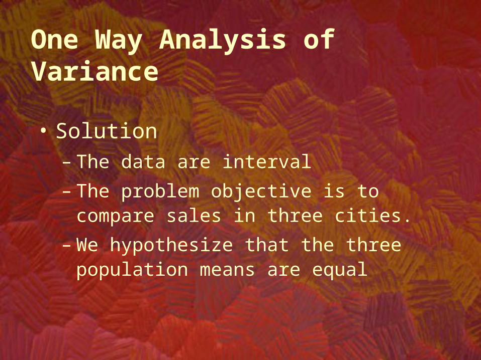
• Solution– The data are interval– The problem objective is to compare sales in three

cities.– We hypothesize that the three population means are

equal


H0: 1 = 2= 3

H1: At least two means differ

To build the statistic needed to test thehypotheses use the following notation:

• Solution

Defining the Hypotheses

Independent samples are drawn from k populations (treatments).

1 2 kX11

x21

.

.

.Xn1,1

1

1x

n

X12

x22

.

.

.Xn2,2

2

2x

n

X1k

x2k

.

.

.Xnk,k

k

kx

n

Sample sizeSample mean

First observation,first sample

Second observation,second sample

X is the “response variable”.The variables’ value are called “responses”.

Notation

Terminology

• In the context of this problem…Response variable – weekly salesResponses – actual sale valuesExperimental unit – weeks in the three cities when we record sales figures.Factor – the criterion by which we classify the populations (the treatments). In this problems the factor is the marketing strategy.Factor levels – the population (treatment) names. In this problem factor levels are the marketing trategies.

Two types of variability are employed when testing for the equality of the population

means

The rationale of the test statistic

Graphical demonstration:Employing two types of variability

20

25

30

1

7

Treatment 1 Treatment 2 Treatment 3

10

12

19

9

Treatment 1Treatment 2Treatment 3

20

161514

1110

9

10x1

15x2

20x3

10x1

15x2

20x3

The sample means are the same as before,but the larger within-sample variability makes it harder to draw a conclusionabout the population means.

A small variability withinthe samples makes it easierto draw a conclusion about the population means.

The rationale behind the test statistic – I

• If the null hypothesis is true, we would expect all the sample means to be close to one another (and as a result, close to the grand mean).

• If the alternative hypothesis is true, at least some of the sample means would differ.

• Thus, we measure variability between sample means.

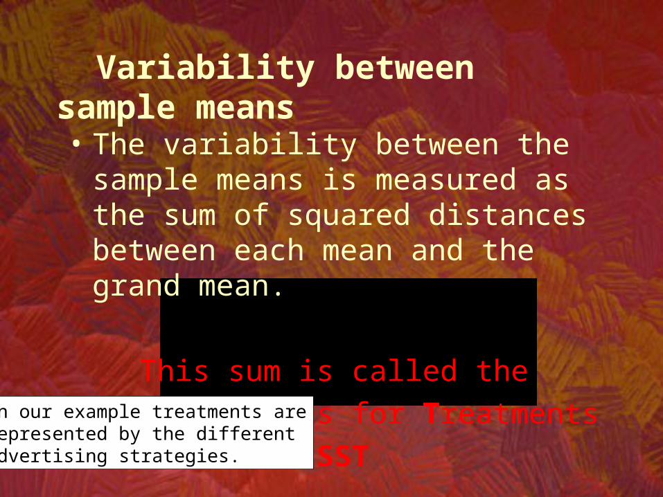
• The variability between the sample means is measured as the sum of squared distances between each mean and the grand mean.

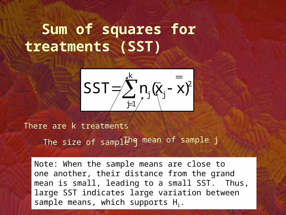
This sum is called the Sum of Squares for Treatments

SSTIn our example treatments arerepresented by the differentadvertising strategies.

Variability between sample means

2k

1jjj )xx(nSST

There are k treatments

The size of sample j The mean of sample j

Sum of squares for treatments (SST)

Note: When the sample means are close toone another, their distance from the grand mean is small, leading to a small SST. Thus, large SST indicates large variation between sample means, which supports H1.

• Solution – continuedCalculate SST

2k

1jjj

321

)xx(nSST

65.608x00.653x577.55x

= 20(577.55 - 613.07)2 + + 20(653.00 - 613.07)2 + + 20(608.65 - 613.07)2 == 57,512.23

The grand mean is calculated by

k21

kk2211

n...nnxn...xnxn

X


Is SST = 57,512.23 large enough to reject H0 in favor of H1?

See next.


• Large variability within the samples weakens the “ability” of the sample means to represent their corresponding population means.

• Therefore, even though sample means may markedly differ from one another, SST must be judged relative to the “within samples variability”.

The rationale behind test statistic – II

• The variability within samples is measured by adding all the squared distances between observations and their sample means.

This sum is called the Sum of Squares for Error

SSEIn our example this is the sum of all squared differencesbetween sales in city j and thesample mean of city j (over all the three cities).

Within samples variability

• Solution – continuedCalculate SSE

Sum of squares for errors (SSE)

k

jjij

n

i

xxSSE

sss

j

1

2

1

23

22

21

)(

24.670,811,238,700.775,10

(n1 - 1)s12 + (n2 -1)s2

2 + (n3 -1)s32

= (20 -1)10,774.44 + (20 -1)7,238.61+ (20-1)8,670.24 = 506,983.50

Is SST = 57,512.23 large enough relative to SSE = 506,983.50 to reject the null hypothesis that specifies that all the means are equal?

Sum of squares for errors (SSE)

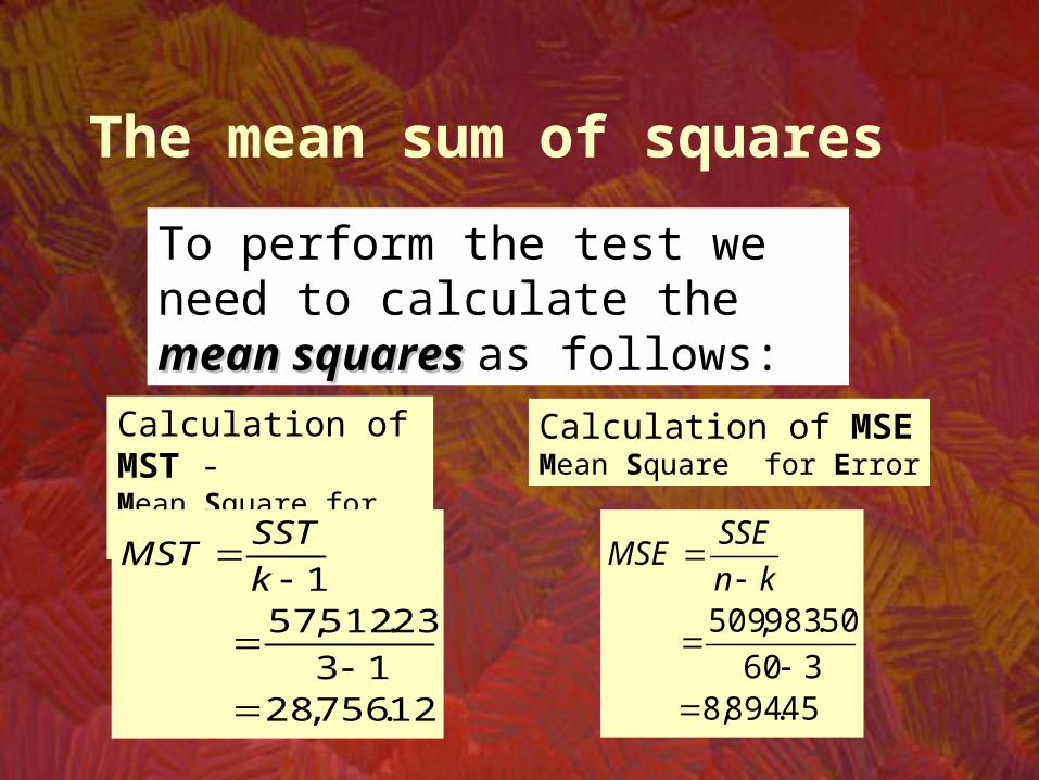
To perform the test we need to calculate the mean squaresmean squares as follows:

The mean sum of squares

Calculation of MST - Mean Square for Treatments

12.756,2813

23.512,571

k

SSTMST

Calculation of MSEMean Square for Error

45.894,8360

50.983,509

kn

SSEMSE

Calculation of the test statistic

23.3

45.894,8

12.756,28

MSE

MSTF

with the following degrees of freedom:v1=k -1 and v2=n-k

Required Conditions:1. The populations tested are normally distributed.2. The variances of all the populations tested are equal.

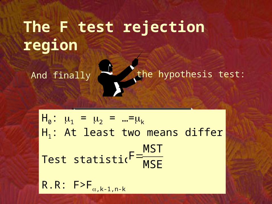
And finally the hypothesis test:

H0: 1 = 2 = …=k


Test statistic:

R.R: F>F,k-1,n-k

MSEMST

F

The F test rejection region

The F test

Ho: 1 = 2= 3


Test statistic F= MST MSE= 3.2315.3FFF:.R.R 360,13,05.0knk 1

Since 3.23 > 3.15, there is sufficient evidence to reject Ho in favor of H1, and argue that at least one of the mean sales is different than the others.

23.317.894,812.756,28

MSEMST

F

-0.02

0

0.02

0.04

0.06

0.08

0.1

0 1 2 3 4

• Use Excel to find the p-value– fx Statistical FDIST(3.23,2,57) = .0467

The F test p- value

p Value = P(F>3.23) = .0467

Excel single factor ANOVA

SS(Total) = SST + SSE

Anova: Single Factor

SUMMARYGroups Count Sum Average Variance

Convenience 20 11551 577.55 10775.00Quality 20 13060 653.00 7238.11Price 20 12173 608.65 8670.24

ANOVASource of Variation SS df MS F P-value F crit

Between Groups 57512 2 28756 3.23 0.0468 3.16Within Groups 506984 57 8894

Total 564496 59

Xm15-01.xls

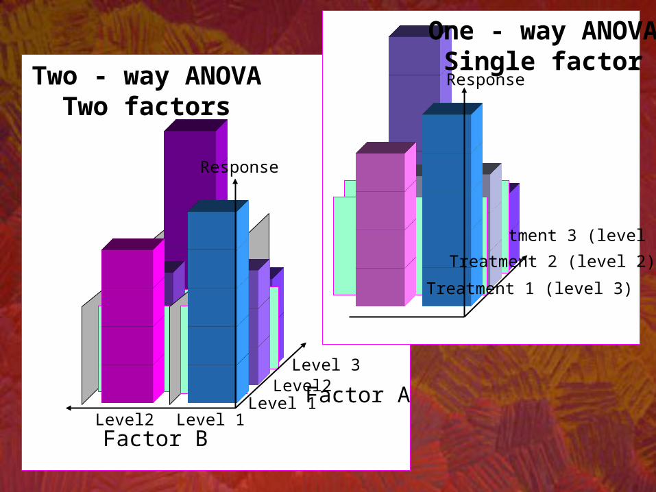
15.3 Analysis of Variance Experimental Designs• Several elements may distinguish between one

experimental design and others.– The number of factors.

• Each characteristic investigated is called a factor.• Each factor has several levels.

Factor ALevel 1Level2

Level 1

Factor B

Level 3

Two - way ANOVATwo factors

Level2

One - way ANOVASingle factor

Treatment 3 (level 1)

Response

Response



• Groups of matched observations are formed into blocks, in order to remove the effects of “unwanted” variability.

• By doing so we improve the chances of detecting the variability of interest.

Independent samples or blocks

• Fixed effects– If all possible levels of a factor are included in our analysis we

have a fixed effect ANOVA.– The conclusion of a fixed effect ANOVA applies only to the

levels studied.• Random effects

– If the levels included in our analysis represent a random sample of all the possible levels, we have a random-effect ANOVA.

– The conclusion of the random-effect ANOVA applies to all the levels (not only those studied).

Models of Fixed and Random Effects

• In some ANOVA models the test statistic of the fixed effects case may differ from the test statistic of the random effect case.

• Fixed and random effects - examples– Fixed effects - The advertisement Example (15.1): All the

levels of the marketing strategies were included – Random effects - To determine if there is a difference in the

production rate of 50 machines, four machines are randomly selected and there production recorded.

Models of Fixed and Random Effects.

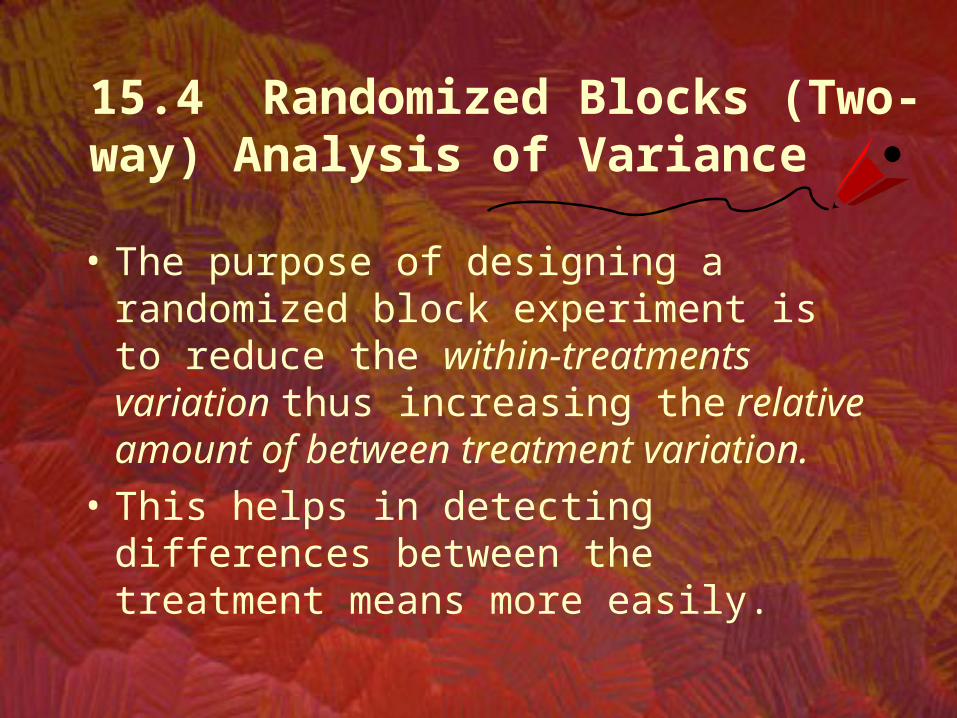
15.4 Randomized Blocks (Two-way) Analysis of Variance

• The purpose of designing a randomized block experiment is to reduce the within-treatments variation thus increasing the relative amount of between treatment variation.

• This helps in detecting differences between the treatment means more easily.

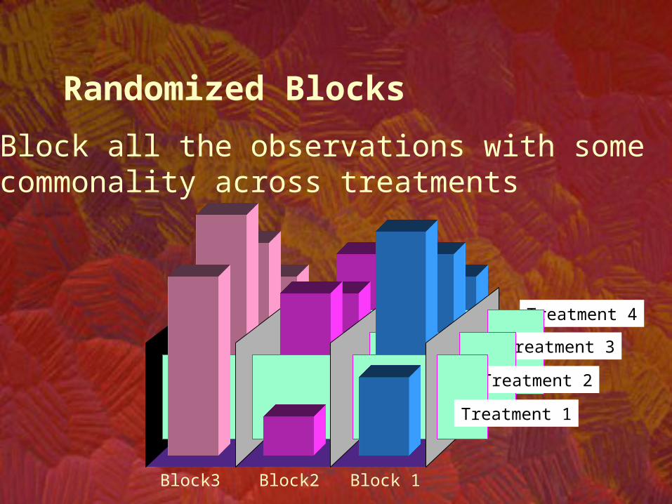
Treatment 4

Treatment 3

Treatment 2

Treatment 1

Block 1Block3 Block2

Block all the observations with some commonality across treatments

Randomized Blocks

TreatmentBlock 1 2 k Block mean

1 X11 X12 . . . X1k2 X21 X22 X2k...b Xb1 Xb2 Xbk

Treatment mean

1]B[x

2]B[x

b]B[x

1]T[x 2]T[x k]T[x

Block all the observations with some commonality across treatments

Randomized Blocks

• The sum of square total is partitioned into three sources of variation– Treatments– Blocks– Within samples (Error)

SS(Total) = SST + SSB + SSESS(Total) = SST + SSB + SSE

Sum of square for treatments Sum of square for blocks Sum of square for error

Recall. For the independent samples design we have: SS(Total) = SST + SSE

Partitioning the total variability

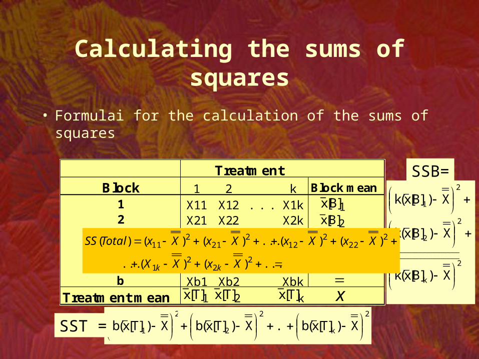
Calculating the sums of squares

• Formulai for the calculation of the sums of squares



Treatment mean

1]B[x

2]B[x

1]T[x 2]T[x k]T[x x2

1 X)]T[x(b

...X)]T[x(b

2

2

2

k X)]T[x(b

SST =

2

1 X)]B[x(k

2

2 X)]B[x(k

2

k X)]B[x(k

SSB=

...)()(...

)()(...)()()(

22

21

222

212

221

211

XxXX

XxXxXxXxTotalSS

kk

Calculating the sums of squares

• Formulai for the calculation of the sums of squares



Treatment mean

1]B[x

2]B[x

1]T[x 2]T[x k]T[x x2

1 X)]T[x(b

...X)]T[x(b

2

2

2

k X)]T[x(b

SST =

2

1 X)]B[x(k

2

2 X)]B[x(k

2

k X)]B[x(k

SSB=

...)X]B[x]T[xx()X]B[x]T[xx(

...)X]B[x]T[xx()X]B[x]T[xx(

...)X]B[x]T[xx()X]B[x]T[xx(SSE

22kk2

21kk1

22222

21212

22121

21111

To perform hypothesis tests for treatments and blocks we need

• Mean square for treatments• Mean square for blocks• Mean square for error

Mean Squares

1kSST

MST

1bSSB

MSB

1bknSSE

MSE

Test statistics for the randomized block design ANOVA

MSEMST

F

MSEMSB

F

Test statistic for treatments

Test statistic for blocks

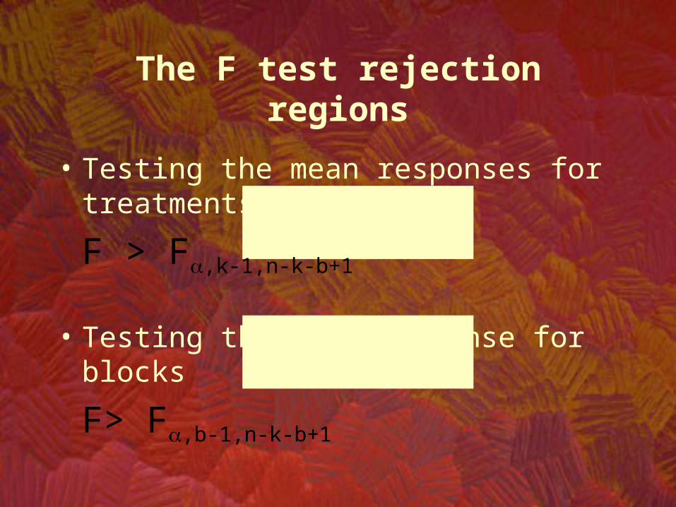
• Testing the mean responses for treatments

F > F,k-1,n-k-b+1

• Testing the mean response for blocks

F> F,b-1,n-k-b+1

The F test rejection regions

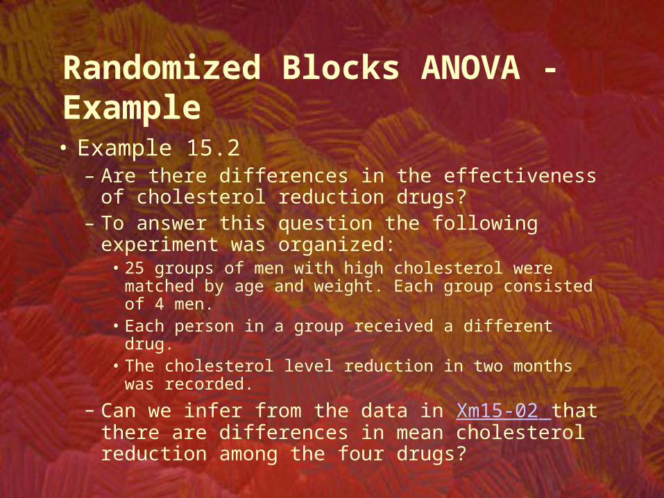
• Example 15.2– Are there differences in the effectiveness of cholesterol

reduction drugs? – To answer this question the following experiment was

organized:• 25 groups of men with high cholesterol were matched by age

and weight. Each group consisted of 4 men.• Each person in a group received a different drug.• The cholesterol level reduction in two months was recorded.

– Can we infer from the data in Xm15-02 that there are differences in mean cholesterol reduction among the four drugs?

Randomized Blocks ANOVA - Example

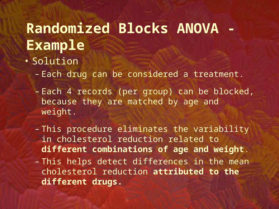
• Solution– Each drug can be considered a treatment.

– Each 4 records (per group) can be blocked, because they are matched by age and weight.

– This procedure eliminates the variability in cholesterol reduction related to different combinations of age and weight.

– This helps detect differences in the mean cholesterol reduction attributed to the different drugs.


BlocksTreatments b-1 MST / MSE MSB / MSE

Conclusion: At 5% significance level there is sufficient evidence to infer that the mean “cholesterol reduction” gained by at least two drugs are different.

K-1


ANOVASource of Variation SS df MS F P-value F critRows 3848.7 24 160.36 10.11 0.0000 1.67Columns 196.0 3 65.32 4.12 0.0094 2.73Error 1142.6 72 15.87

Total 5187.2 99

Analysis of VarianceAnalysis of Variance

Chapter 15 - continued

15.5 Two-Factor Analysis of Variance -

• Example 15.3– Suppose in Example 15.1, two factors are to be

examined:• The effects of the marketing strategy on sales.

– Emphasis on convenience– Emphasis on quality– Emphasis on price

• The effects of the selected media on sales.– Advertise on TV– Advertise in newspapers

• Solution– We may attempt to analyze combinations of levels, one

from each factor using one-way ANOVA.– The treatments will be:

• Treatment 1: Emphasize convenience and advertise in TV• Treatment 2: Emphasize convenience and advertise in

newspapers• …………………………………………………………………….• Treatment 6: Emphasize price and advertise in newspapers

Attempting one-way ANOVA

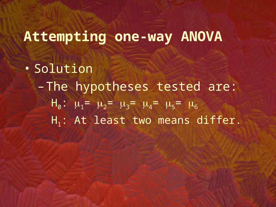
• Solution– The hypotheses tested are:

H0: 1= 2= 3= 4= 5= 6

H1: At least two means differ.


City1 City2 City3 City4 City5 City6Convnce Convnce Quality Quality Price Price

TV Paper TV Paper TV Paper

– In each one of six cities sales are recorded for ten weeks. – In each city a different combination of marketing emphasis and media usage is employed.

• Solution


• The p-value =.0452. • We conclude that there is evidence that differences exist in the mean weekly sales among the six cities.

City1 City2 City3 City4 City5 City6Convnce Convnce Quality Quality Price Price

TV Paper TV Paper TV Paper

• Solution

Xm15-03


• These result raises some questions:– Are the differences in sales caused by the different

marketing strategies?– Are the differences in sales caused by the different

media used for advertising?– Are there combinations of marketing strategy and

media that interact to affect the weekly sales?

Interesting questions – no answers

• The current experimental design cannot provide answers to these questions.

• A new experimental design is needed.

Two-way ANOVA (two factors)


City 1sales

City3sales

City 5sales

City 2sales

City 4sales

City 6sales

TV

Newspapers

Convenience Quality Price

Are there differences in the mean sales caused by different marketing strategies?

Factor A: Marketing strategy

Fact

or B

: Ad

verti

sing

med

ia

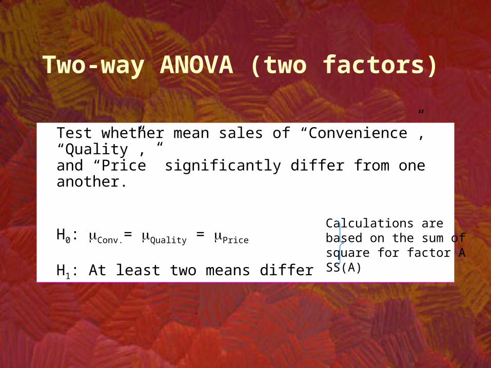
Test whether mean sales of “Convenience”, “Quality”, and “Price” significantly differ from one another.

H0: Conv.= Quality = Price


Calculations are based on the sum of square for factor ASS(A)



City 1sales

City 3sales

City 5sales

City 2sales

City 4sales

City 6sales


Fact

or B

: Ad

verti

sing

med

ia

Are there differences in the mean sales caused by different advertising media?

TV

Newspapers


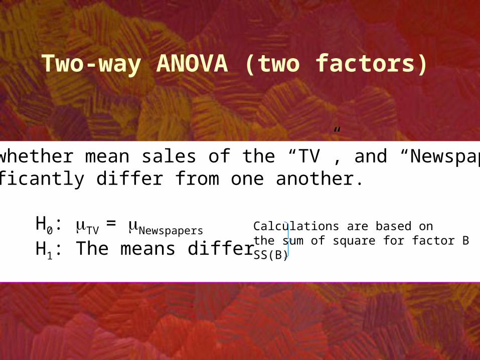
Test whether mean sales of the “TV”, and “Newspapers” significantly differ from one another.

H0: TV = Newspapers

H1: The means differ

Calculations are based onthe sum of square for factor BSS(B)



City 1sales

City 5sales

City 2sales

City 4sales

City 6sales

TV

Newspapers



Fact

or B

: Ad

verti

sing

med

ia

Are there differences in the mean sales caused by interaction between marketing strategy and advertising medium?

City 3sales

TV

Quality

Test whether mean sales of certain cells are different than the level expected.

Calculation are based on the sum of square for interaction SS(AB)


Graphical description of the possible relationships between factors A and B.Graphical description of the possible relationships between factors A and B.

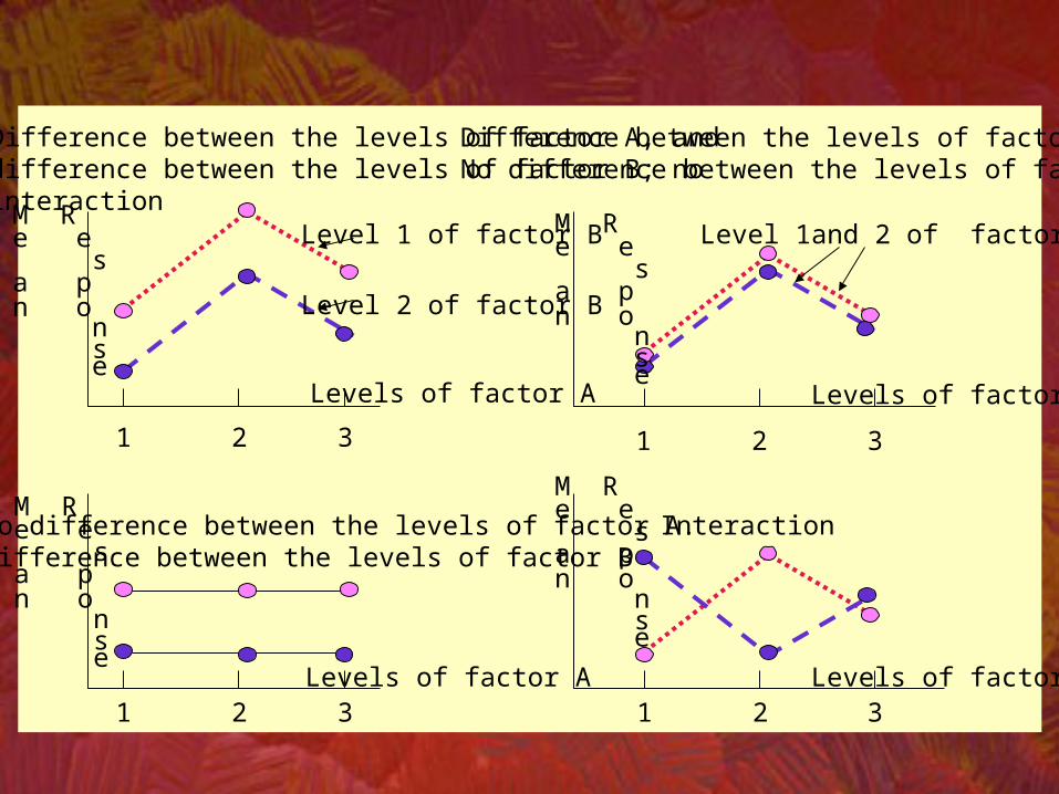
Levels of factor A

1 2 3

Level 1 of factor B

Level 2 of factor B

1 2 3

1 2 31 2 3

Level 1and 2 of factor B

Difference between the levels of factor ANo difference between the levels of factor B

Difference between the levels of factor A, anddifference between the levels of factor B; nointeraction

Levels of factor A

Levels of factor A Levels of factor A

No difference between the levels of factor A.Difference between the levels of factor B

Interaction

M Re e sa pn o n s e




Sums of squares

a

1i

2i )x]A[x(rb)A(SS })()()){(2(10( 222

. xxxxxx pricequalityconv

b

1j

2j )x]B[x(ra)B(SS })()){(3)(10( 22 xxxx NewspaperTV

b

1j

2jiij

a

1i

)x]B[x]A[x]AB[x(r)AB(SS

r

kijijk

b

j

a

i

ABxxSSE1

2

11

)][(

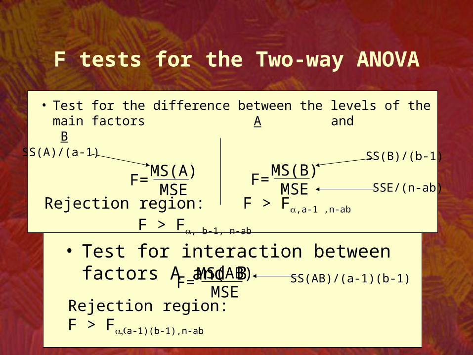
F tests for the Two-way ANOVA

• Test for the difference between the levels of the main factors A and B

F= MS(A)MSE

F= MS(B)MSE

Rejection region: F > F,a-1 ,n-ab F > F, b-1, n-ab

• Test for interaction between factors A and B

F= MS(AB)MSE

Rejection region: F > Fa-1)(b-1),n-ab

SS(A)/(a-1) SS(B)/(b-1)

SS(AB)/(a-1)(b-1)

SSE/(n-ab)

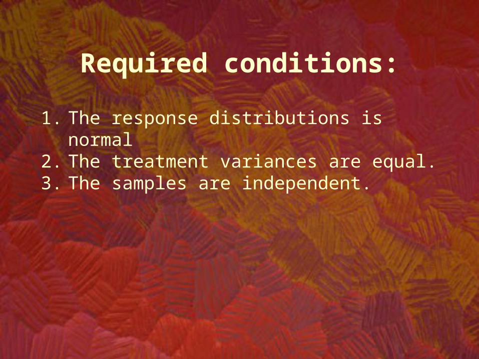
Required conditions:

1. The response distributions is normal2. The treatment variances are equal.3. The samples are independent.

• Example 15.3 – continued( Xm15-03)



TV 491 677 575TV 712 627 614TV 558 590 706TV 447 632 484TV 479 683 478TV 624 760 650TV 546 690 583TV 444 548 536TV 582 579 579TV 672 644 795

Newspaper 464 689 803Newspaper 559 650 584Newspaper 759 704 525Newspaper 557 652 498Newspaper 528 576 812Newspaper 670 836 565Newspaper 534 628 708Newspaper 657 798 546Newspaper 557 497 616Newspaper 474 841 587

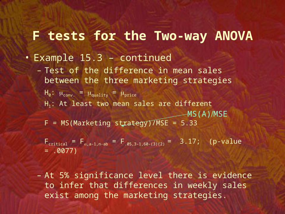
• Example 15.3 – continued– Test of the difference in mean sales between the three marketing

strategiesH0: conv. = quality = price

H1: At least two mean sales are different


ANOVASource of Variation SS df MS F P-value F critSample 13172.0 1 13172.0 1.42 0.2387 4.02Columns 98838.6 2 49419.3 5.33 0.0077 3.17Interaction 1609.6 2 804.8 0.09 0.9171 3.17Within 501136.7 54 9280.3

Total 614757.0 59

Factor A Marketing strategies

• Example 15.3 – continued– Test of the difference in mean sales between the three

marketing strategiesH0: conv. = quality = price

H1: At least two mean sales are different

F = MS(Marketing strategy)/MSE = 5.33

Fcritical = F,a-1,n-ab = F.05,3-1,60-(3)(2) = 3.17; (p-value = .0077)

– At 5% significance level there is evidence to infer that differences in weekly sales exist among the marketing strategies.


MS(A)MSE

• Example 15.3 - continued– Test of the difference in mean sales between the two

advertising mediaH0: TV. = Nespaper

H1: The two mean sales differ


Factor B = Advertising media


Total 614757.0 59

• Example 15.3 - continued– Test of the difference in mean sales between the two

advertising mediaH0: TV. = Nespaper

H1: The two mean sales differ

F = MS(Media)/MSE = 1.42 Fcritical = Fa-1,n-ab = F.05,2-1,60-(3)(2) = 4.02 (p-value = .2387)

– At 5% significance level there is insufficient evidence to infer that differences in weekly sales exist between the two advertising media.


MS(B)MSE

• Example 15.3 - continued– Test for interaction between factors A and B

H0: TV*conv. = TV*quality =…=newsp.*price



Interaction AB = Marketing*Media


Total 614757.0 59

• Example 15.3 - continued– Test for interaction between factor A and B

H0: TV*conv. = TV*quality =…=newsp.*price


F = MS(Marketing*Media)/MSE = .09

Fcritical = Fa-1)(b-1),n-ab = F.05,(3-1)(2-1),60-(3)(2) = 3.17 (p-value= .9171)

– At 5% significance level there is insufficient evidence to infer that the two factors interact to affect the mean weekly sales.

MS(AB)MSE


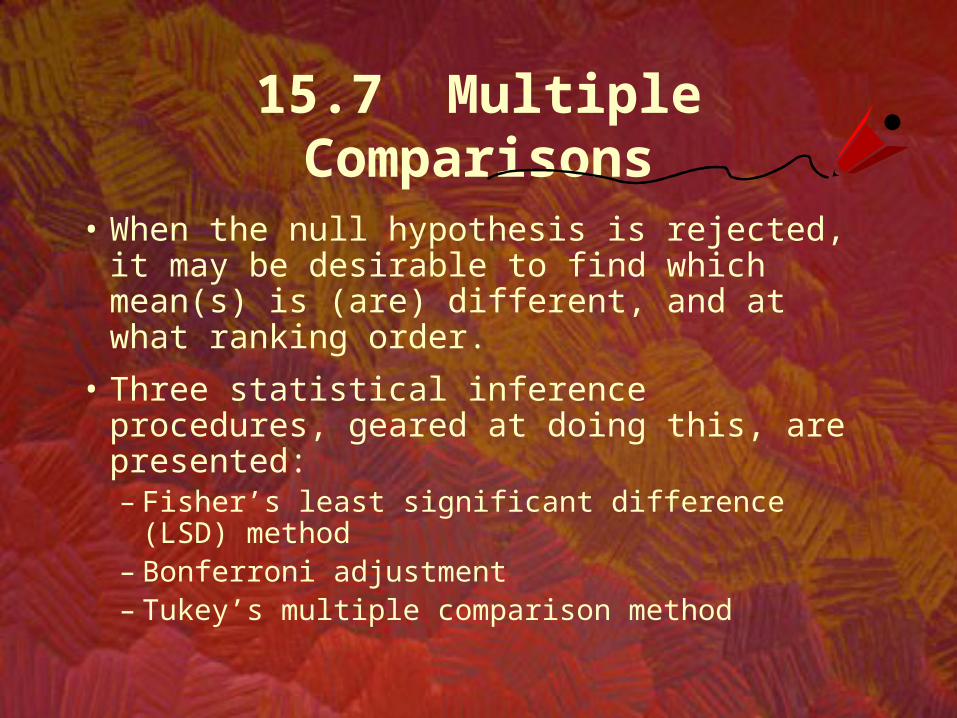
15.7 Multiple Comparisons

• When the null hypothesis is rejected, it may be desirable to find which mean(s) is (are) different, and at what ranking order.

• Three statistical inference procedures, geared at doing this, are presented:– Fisher’s least significant difference (LSD) method– Bonferroni adjustment– Tukey’s multiple comparison method

• Two means are considered different if the difference between the corresponding sample means is larger than a critical number. Then, the larger sample mean is believed to be associated with a larger population mean.

• Conditions common to all the methods here:– The ANOVA model is the one way analysis of variance– The conditions required to perform the ANOVA are satisfied.– The experiment is fixed-effect

15.7 Multiple Comparisons

Fisher Least Significant Different (LSD) Method

• This method builds on the equal variances t-test of the difference between two means.

• The test statistic is improved by using MSE rather than sp2.

• We can conclude that i and j differ (at % significance level if |i - j| > LSD, where

kn.f.d

)n1

n1

(MSEtLSDji

2

Experimentwise Type I error rate (E)(the effective Type I error)

• The Fisher’s method may result in an increased probability of committing a type I error.

• The experimentwise Type I error rate is the probability of committing at least one Type I error at significance level of It iscalculated by

E = 1-(1 – )C

where C is the number of pairwise comparisons (I.e. C = k(k-1)/2

• The Bonferroni adjustment determines the required Type I error probability per pairwise comparison () , to secure a pre-determined overall E

• The procedure:– Compute the number of pairwise comparisons (C)

[C=k(k-1)/2], where k is the number of populations.– Set = E/C, where E is the true probability of making at

least one Type I error (called experimentwise Type I error).– We can conclude that i and j differ (at /C% significance

level if

kn.f.d

)n1

n1

(MSEtji

)C2(ji

Bonferroni Adjustment

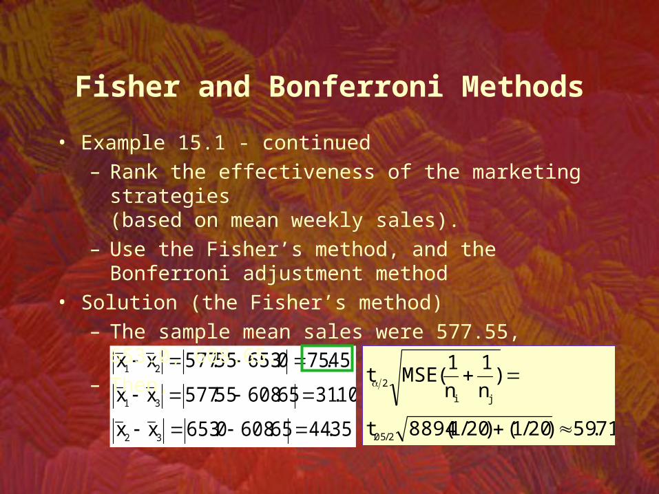
35.4465.6080.653xx

10.3165.60855.577xx

45.750.65355.577xx

32

31

21

• Example 15.1 - continued– Rank the effectiveness of the marketing strategies

(based on mean weekly sales).– Use the Fisher’s method, and the Bonferroni adjustment method

• Solution (the Fisher’s method)– The sample mean sales were 577.55, 653.0, 608.65.– Then,

71.59)20/1()20/1(8894t

)n1

n1

(MSEt

2/05.

ji

2

Fisher and Bonferroni Methods

• Solution (the Bonferroni adjustment)– We calculate C=k(k-1)/2 to be 3(2)/2 = 3.– We set = .05/3 = .0167, thus t.01672, 60-3 = 2.467 (Excel).

54.73)20/1()20/1(8894467.2

)n1

n1

(MSEtji

2

Again, the significant difference is between 1 and 2.

35.4465.6080.653xx

10.3165.60855.577xx

45.750.65355.577xx

32

31

21

Fisher and Bonferroni Methods

• The test procedure:– Find a critical number as follows:

gnMSE

),k(q

k = the number of samples =degrees of freedom = n - kng = number of observations per sample (recall, all the sample sizes are the same) = significance levelq(k,) = a critical value obtained from the studentized range table

Tukey Multiple Comparisons

If the sample sizes are not extremely different, we can use the above procedure with ng calculated as the harmonic mean ofthe sample sizes. k21 n1...n1n1

kgn

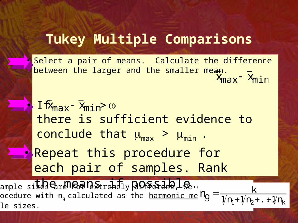
• Repeat this procedure for each pair of samples. Rank the means if possible.

• Select a pair of means. Calculate the difference between the larger and the smaller mean.

• If there is sufficient evidence to conclude that max > min .

minmax xx

minmax xx


City 1 vs. City 2: 653 - 577.55 = 75.45City 1 vs. City 3: 608.65 - 577.55 = 31.1City 2 vs. City 3: 653 - 608.65 = 44.35

• Example 15.1 - continued We had three populations (three marketing strategies).K = 3,

Sample sizes were equal. n1 = n2 = n3 = 20,= n-k = 60-3 = 57,MSE = 8894.

minmax xx

70.7120

8894)57,3(.q

nMSE

),k(q 05g

Take q.05(3,60) from the table.

Population

Sales - City 1Sales - City 2Sales - City 3

Mean

577.55653698.65

minmax xx


Excel – Tukey and Fisher LSD method

Xm15-01

Fisher’s LDS

Bonferroni adjustments

= .05

= .05/3 = .0167

Multiple Comparisons

LSD OmegaTreatment Treatment Difference Alpha = 0.05 Alpha = 0.05Convenience Quality -75.45 59.72 71.70

Price -31.1 59.72 71.70Quality Price 44.35 59.72 71.70

Multiple Comparisons

LSD OmegaTreatment Treatment Difference Alpha = 0.0167 Alpha = 0.05Convenience Quality -75.45 73.54 71.70

Price -31.1 73.54 71.70Quality Price 44.35 73.54 71.70

Anova (1)

Education

Transcript of Anova (1)