G. B. WALLIS Associate Professor,

Thayer School of Engineering, Dartmouth Col lege,

Hanover, N. H. Assoc. Mem. ASME; Also, Creare, Inc.,

Hanover, N . H.

Annular Two-Phase Flow Fart 1: A Simple Theory A simple theory for annular two-phase flow is developed in terms of equations for the interfacial and wall shear stresses. Expressions for the pressure drop and void fraction are derived. Criteria for the minim-urn, pressure drop, zero wall shear, and flow regime transition in vertical flow are given. The results are compared with numerous data and alternative theories from the literature.

%

Introduction

Jp TO now there have been two approaches to annular flow which were generally available to the engineer. The first was the use of some very crude, but easy-to-use, correlations such as Martinelli's or the various versions of homogeneous flow theory. The second was the piecing together of a calculation procedure from analyses or correlations of parts of the flow which have been described in some detail by research workers.

The disadvantage of both techniques is that neither provides a conceptual framework within which the whole picture can be de­veloped with appropriate sophistication. Sweeping correlations suffer from their basic inflexibility, a lack of relationship to meaningful physical phenomena, and the awkwardness of adapting them to take account of secondary effects. The synthesizing of many bits and pieces of scientific work, on the other hand, is arduous and quite often becomes a research topic in itself. The nonspecialist just does not have the time to stud}' the ways in Tvhich the theories of many different authors are related.

The objective of the first of these two papers is to jjresent a theory of annular flow which is sufficiently simple to be useful and, at the same time, is based on the major physical phenomena which occur. Comparison is made with a wide variety of data and with other theories from the literature which can be rearranged into a similar form. Because the parameters in the theory are physi­cally motivated, they are readily related to more complex analyses by means of correction factors. This is done in the second paper [18]' in which several more specialized investigations are interpreted in terms of the overall conceptual structure. Thus the simple theory is like the apex of a pyramid which stands on a

1 Numbers in brackets designate References at end of paper. Contributed by the Fluids Engineering Division and presented at

the Applied Mechanics and Fluids Engineering Conference, Evans-ton, 111., June 16-18, 1969, of THE AMERICAN SOCIETY OP MECHANI­CAL ENGINEERS. Manuscript received at ASME Headquarters, March 20, 1969. Paper No. 69-FE-45.

framework composed of more thorough scientific studies. Hope­fully, additional information can be inserted into this pyramid a t suitable levels as it is developed. Thus it is easier to grasp the significance of new information.

Development of a Simple Theory for Vertical Annular Flow Qualitative Aspects. Vertical annular flow resembles the sketch

shown in Fig. 1. Gas, which may contain suspended droplets, flows in a central core, while liquid flows in an annular film. The interface between the gas and the liquid usually appears wavy, and much of the interfacial shear stress, r,-, is due to form drag on these waves. If the film has a mean thickness, 5, the fraction of the cross section which it occupies is

D

z

LIQUID

Fig. 1 Sketch of vertical annular flow

•Nomenclature-

D = pipe diameter / = friction factor

F1 = Levy parameter [see equation (36)] (j = acceleration due to gravity O = mass flux j = volumetric flux

7c, = sand roughness p = pressure Q = volumetric flow rate B = Levy parameter [see equation

(36)] V — velocity z = distance down pipe

a = void fraction 5 = film thickness

u = viscosity p = density T = shear stress

4>g = Martinelli parameter

Subscripts

c = core / = liquid g = gas i = interface

w — wall

Dimensionless Groups

jf* = turbulent liquid flux, equation (25)

hl

N, =

laminar liquid flux, equation

(26)

turbulent gas flux, equation (24)

liquid viscosity, equation (31) AP* =

Re/ =

pressure drop, equation (23)

liquid Reynolds number, tion (30)

Abbrev/af/ons

CISE

UKAEA

= Centro informazioni esperienze, Segrate, Italy

equa-

studi Milan,

= United Kingdom Atomic En­ergy Authority

journal of Basic Engineering MARCH 1 9 7 0 / 59 Copyright © 1970 by ASME

SLUG FLOW

( I - (X) LIQUID FRACTION

Fig. 2 Qualitative aspects of pressure-drop characteristics of various flow regimes

(1 - a ) 1 -(D - 25)2

D2 ib-The mean diameter of the gas stream is

D\/a> = D - 25

(1)

(2)

Suppose that one treats the gas stream as flowing in a "rough" pipe with walls composed of the interface. By analogy with single-phase flow, we define a fraction factor, /,•, by the relation­ship

A = l / 2 p ^ , '

(3)

The interface has been assumed to be stationary since, in most cases, V 0 S> Y ;.

Performing a force balance for the central core of the flow, we find, in the absence of compressibility effects and area change

dp

dz

whence, from equation (3)

Pa3 + Dy/o

0

— dp

dz PJ=fil/2p.V,*--J D\/o

(4)

(5)

In most cases, dp/dz 2> pgg, and the friction factor can be ex pressed as

-dp/dz Z>V'a fi = 2p,V,

(6)

Usually one does not know Va directly, but only the gas volumetric flow rate Q„ and the "void fraction" a. The mean volumetric gas flux, j g , is defined to be

h = irD2

The mean gas velocity then follows as

and equation (6) becomes

/,• =

V = ^L

— dp/dz- D- a •h

2p„i„2

(V)

(8)

(9)

Fig. 2 shows a plot of the interfacial friction factor versus liquid fraction for both upflow, horizontal flow, and downflow, and serves to indicate the various regimes of flow.

In horizontal or downflow at low gas velocities, the liquid film is smooth and the friction factor is approximately the smooth pipe value. Above a critical gas velocity for wave inception, the friction factor rises rapidly to a maximum after which it tends to follow the line marked "rough annular flow." The onset of waves is dependent on the surface tension, among other variables, and has not been successfully rationalized yet. At higher gas veloci­ties, the tops of the waves are sheared off to form entrained drop­lets and the density of the core increases. This leads to an in­crease in the friction factor, defined by equation (9), in about the ratio pclp„, where pe is now the average homogeneous density of the core.

At very high flow rates of both phases, almost all of the liquid flow is entrained, and the pressure drop is given by "homogeneous" flow theoiy as

— dp

dz = f-j,[0, + C

2

"15 (10)

The symbol O represents the mass flow rate divided by the total pipe area. Equation (10) can be rearranged to give

— dp

dz fPgh* 1 + 2/ 2_

1) In homogeneous flow the liquid fraction is

(11)

(12) Qf + Qo

Usually the volumetric flow rate of the gas is much greater than the liquid flow rate, and equation (12) can be approximated by

Q„ P/ G„

Using equation (13) in equation (11), we find that

(13)

— dp

dz • fPoJo 1 + ^ ( 1 a) 2^

D (14)

,5A (15)

If the friction factor in homogeneous flow is relatively unchanged from the value for gas alone, /„, .[as it usually is] we can use equation (14) to show that

-dp/dz-D-a'/* r p, ' ^ ~ 7 1 =fa 1 + — (1 - a ) 2p„;0

2 L p„

For air and water at atmospheric pressure Pj/p„ a 800 and for homogeneous flow, the value of equation (15) increases very rapidly as a fraction of (1 — a), as shown in Fig. 2. The curves tend to move toward the homogeneous flow line as the liquid rate is increased and the percent entrained goes up accordingly.

In vertical flow, the interfacial shear has to support the film

60 / M A R C H 1970 Transactions of the ASME

.ObZ5

<

,0 .05

2 2.0375 O

m \ .025

(k

.0125

.OOS

-

-

-

^ D * rf£

O © A D

A

9

MARTIHELLI l"DIA. HORIZONTAL. DUKLER 1*DIA. VERTICAL. SZE FOO CHIEN Z"DIA. VERTICAL. . CHARVONIA 3"DIA. VERTICAL.

A

L\y^S A J*

A J ^ O O A ^€ 8

o-<# • ®e

i , i

J^ •/?*

^

EQUATION (16)

EQUATION (17)

1 , 1

DIMENSIONLESS FILM THICKNESS

Fig. 3 Comparison between equations (16) and (17) and air-water data

against gravity. Furthermore, any slugs of liquid or entrained droplets add a gravitational component to the core pressure drop. Thus, at low gas rates in the slug flow region, the "friction factor" defined by equation (9) increases well above the annular flow value. At lower liquid rates this is usually at values of liquid fraction above about 0.2. At high liquid rates, the transition between slug flow and annular mist flow becomes obscure and there is a general motion toward the homogeneous flow line.

Interracial Shear Stress. The interfacial shear stress has been dis­cussed by many authors and is usually represented in a rather complicated way. The key to the present analysis is a simple plot of the interfacial friction factor versus the dimensionless film thickness, as shown in Fig. 3. The points cluster pretty well around a line with equation

U = 0.005 1 300-D

(16)

In view of equation (1), this is approximately the same as

/,. = 0.005[1 + 75(1 - a)} (17)

We note at this point that the rough pipe correlations of Nikuradse [3] and Moody [4] can be approximated by the equa­tion

K 1 + 75 / « 0.005

D (18)

over the range 0.001 < kJD < 0.03, where k„ is the grain size of a "sand roughness." Equation (16), therefore, shows that a wavy annular film is about equivalent to a sand roughness of four times the film thickness.

Using equations (16), (8), and (3) in equation (4), we obtain

dp

dz + P/J) = 10- D

[1 + 75(1 - a)] (19)

Another way to look at equation (19) (apart from the small gravitational term) is to say that the pressure drop is increased above the value for the gas alone in the pipe by a factor, <£„', which was originally introduced by Martinelli [5]. Taking the friction factor for the gas alone as 0.005, we readily obtain

[1 + 75(1 - a ) ] 1 / 2

?h (20)

Fig. 4 shows that equation (20) is intermediate between several expressions which are due to other authors.

Turner [6], among others, has shown that it is reasonable to as­sume that the wall shear stress is the same as it would be if the liquid film were part of a liquid stream filling the whole pipe. In turbulent flow, with a wall friction factor of 0.005, a force balance on the whole flow gives

dp

dz + PS (1 - «)(p, - pg)g + 10-» ^ f ^ 2 (21) D{1 — a)'

In the case of laminar flow, it is more accurate to solve the dif­ferential equations across the film to get the result

dp

dz + P/J 32

+

J / M / B 2 ( l - aY

2a2 In a 1 -

(1 - a ) 2

2a

1 - a 3(pf - P„) (22)

The final square bracket in equation (22) can be closely approxi­mated [6] over the range D < (1 - a) < 0.2 by the value (0.684) (1 - a ) .

I t is convenient at this point to define dimensionless forms of the pressure drop and flow rates as follows

AP* = - [dp/dz + pgg]

0(P/ - P„) (23)

•eta

- MARTINELLI S CORRELATION -TURNER 'S EMPIRICAL RESULTS FOR ANNULAR

•> SEMI-ANNULAR FLOW — TURNERS ANALYSIS ('/ylhPOWER PROFILE) -PRESENT THEORY

O.G5 O.IQ

(l-Ct) LIQ.UIO FRACTION

Fig. 4 Expression of present theory in terms of Martinelli's parameter c

Journal of Basic Engineering MARCH 1 9 7 0 / 61

-.5 .05 JO .15

Fig, 5 / / * versus (1 — a) for various values of /'„* for a turbulent film

.20

AP*

Fig. 6 Dimensionless pressure drop AP* versus dimensionless gas flux ig*, for various values o f / / * (turbulent film)

• * _ IsRl [gD(P; ~ p,)]V

; * = ilPUl [gD(p, - p„)]V

3 % > /

(24)

(25)

(26) Fig. 7 Enlargement of Fig. 6 for low values of /"/*

D>g(pf - p0)

In terms of these parameters, equations (19), (21), and (22) become

1 + 75(1 - a)

Laminar AP* = jfl* (1 - a)'

+ (0.684)(1 - a) (29)

AP* = 1 0 ~ V *

Turbulent AP* = (1 - a) + 10"

(27)

(1 - a ) 2

If the turbulent flow solution could be obtained by a differential analysis of the film, the first term on the right-hand side of equa-

(28) tion (28) would presumably be slightly modified. The liquid film Reynolds number is

62 / M A R C H 1970 Transactions of the ASME

s -

x*= a5

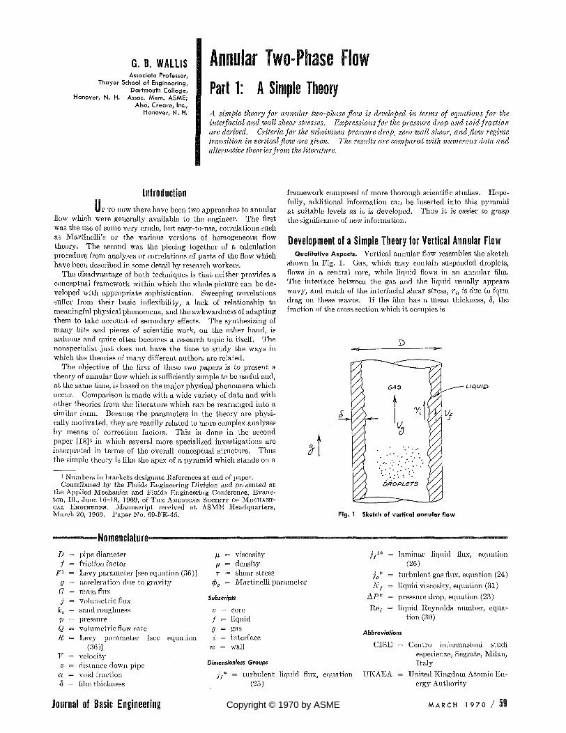
Fig. 8 / / * versus (1 — a) for various values of / „ * (laminar film)

s Q

4 ° 0.3

VALUES OF jf A

e,io~'

Jj

0.5 I.O 1.5 * DIMSNS/ONLESS SAS FLUX

Fig. 9 AP* versus /'„* for various values of / / * (laminar film)

R e / = M/

(30)

AT, =

A further useful dimensionless quantity is

A/

I t is readily found that

R e , = jj*N,

and

(P, - P 9 ) ' A (31)

(32)

i / * = 32j,*/Nf (33)

Equations (27)-(29) were solved on the Dartmouth GE 235 computer for numerous vahies of the parameters by Andrew

Ap*xio~*

Fig. 10 Detail of Fig. 9 at low values of / ' / ' *

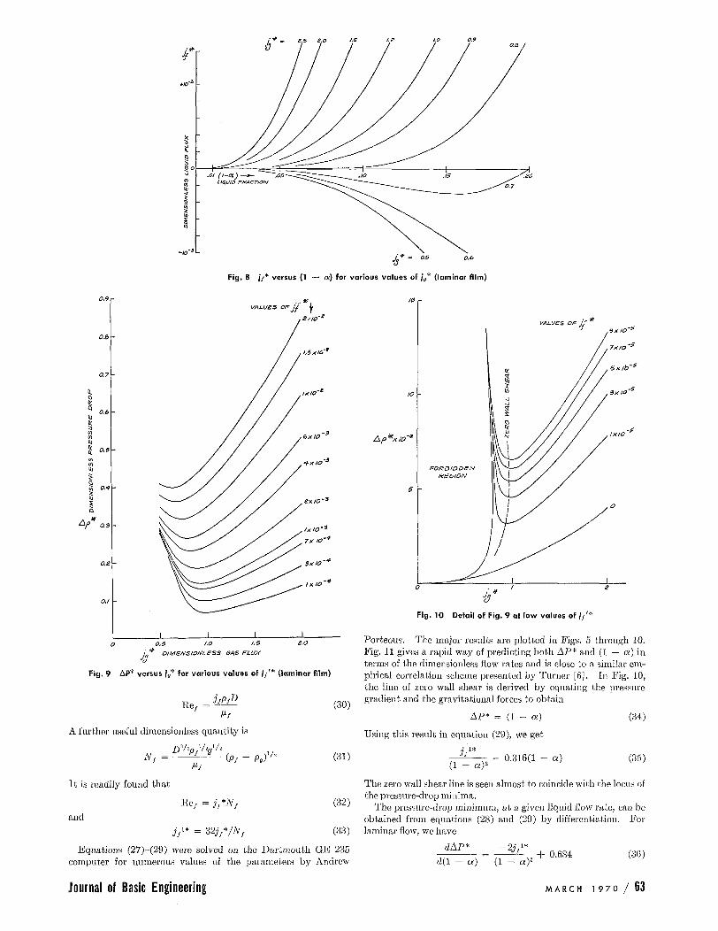
Porteous. The major results are plotted in Figs. S through 10. Fig. 11 gives a rapid way of predicting both AP* and (1 — a) in terms of the dimensionless flow rates and is close to a similar em­pirical correlation scheme presented by Turner [6]. In Fig. 10, the line of zero wall shear is derived by equating the pressure gradient and the gravitational forces to obtain

AP* = (1 - a)

Using this result in equation (29), we get

A 1# Js

(1 - a ) 2 0.316(1 - a )

(34)

(35)

The zero wall shear line is seen almost to coincide with the locus of the pressure-drop minima.

The pressure-drop minimum, a t a given liquid Bow rate, can be obtained from equations (28) and (29) by differentiation. For laminar flow, we have

dAP* -%"/' rf(l - a) (1 - a)3 + 0.684 (36)

Journal of Basic Engineering M A R C H 1 9 7 0 / 63

0.0baof-08aog 0J0 a// OJS A IS O.lf Q/S

Fig. 11 AP* and (1 — a) as functions of jg*% and / / * 2 (turbulent film)

o.os o

™ ^ ^ y i0

er y if / 7 y /

lo-4 1

o

y y

A

o

1 1

.us:' A ^ "

Ret * 300O - - &

1 ^-'-'^ _^ " " "

TURBULENT Flt-M

DATA. J,*** /•& HEWITT, KINS, AND LOVEGROVE;

DATA. j * - ^ l . b HEWITT ANP LOVESROVEi O

Sx/o"* 1. 7xlQ~ 1 Jf 1

1 1 / *

Fig. 12 Comparison between present theory andjclata of Hewitt, King, and Lovegrove ( I . 25 - in . dia, air-water » 15 psia)

LAMINAR FlLfrt

7URaUL£NT FILM

Fig. 13 Comparison between present theory and data of Hewitt, King, and Lovegrove (1.25-in. dia, air-water « 15 psia)

64 / MARCH 1 970 Transactions of the AS ME

The minimum occurs when

It1 0.342(1 - a)s (37)

(38)

(39)

Since equations (38) and (39) are almost exactly compatible with equation (34), and equations (35) and (37) are much the same, the pressure-drop minimum is indeed very close to the point of zero wall shear.

For turbulent flow, a similar treatment of equation (28) gives, at the minimum pressure drop

(1 - a) = 1.43J/*1/3

The corresponding value of the pressure drop is

APm i„* = 1.47i/*'/3

(1 -

AP • " i mm

a) = 0.272j/*2/3

0-41.77

(40)

(41)

In general, for a friction factor of fm instead of the assumed value of 0.005, the results are

(1 - a) = 0.272 0.005

•A

If

APrr 0.41 \ 0 . 0 0 5 / 3f *

2A

(42)

(43)

Thus an increase in wall friction factor increases the minimum pressure drop.

Several important qualitative aspects of the graphs deserve attention. First, it is evident from Fig. 5 that the character of the flow changes quite dramatically when j g * falls below about unity. No downflow is possible unless jg* is less than 0.95, and a slight reduction below this value requires high liquid fractions before upflow can occur. (There is actually a slight region of upflow near the origin which only a l lows^* values below 0.01.) Practically, a value of j a * = 0.9 corresponds to a situation in which thin liquid films flow downward while thick ones flow upward. A net upflow of liquid then usually occurs as a result of "waves" of thick film riding over a smoother and thinner falling film. With values of jg* below 0.9, these thick films are usually sufficient to bridge the pipe temporarily and bring about a transition to slug flow. This conclusion is consistent with the empirical conclusion of Wallis [7] that the onset of annular upflow at low liquid rates occurs between jg* = 0.8 and 0.9.

In the case of laminar flow, Fig. 8, the picture is much the same with the transition occurring at jg* = 0.8.

The pressure-drop graphs for low liquid rates, Figs. 7 and 10, display the same effects in a different way. Below a gas rate in the range 0.8 < jg* < 1, the pressure drop increases immensely and there is a "forbidden region" in which no solutions can be obtained. Since one is often dealing in practice with systems in which the pressure drop is controlled by the external charac­teristics, this forbidden region can be very significant since an attempt to operate in it results in either a new flow regime or an unstable situation in which a large change in the operating conditions occurs. Moreover, at a gas flux which crosses this forbidden region at low liquid flow rates, there are +hree possible solutions to the pressure drop for a given liquid rate. Rather small fluctuations in any one of the parameters can then lead to a jump from the low-pressure drop to the high-pressure drop value.

The pressure-drop minimum at a constant liquid rate is also of significance for determining the stability of a system in which the pressure drop and liquid rate are controlled. If the gas rate is allowed to fall below the value corresponding to the minimum pressure drop, it will continue to fall until the pipe fills with liquid and becomes flooded.

In general, the first-order stability of any system will be deter­mined by the interaction between these pressure-drop charaeter-

WITT, KINQ, AND LOVEGROVE A DATA j * J.

O DATA j * — 4.0 HEWITT AND LOVECfKCK/E

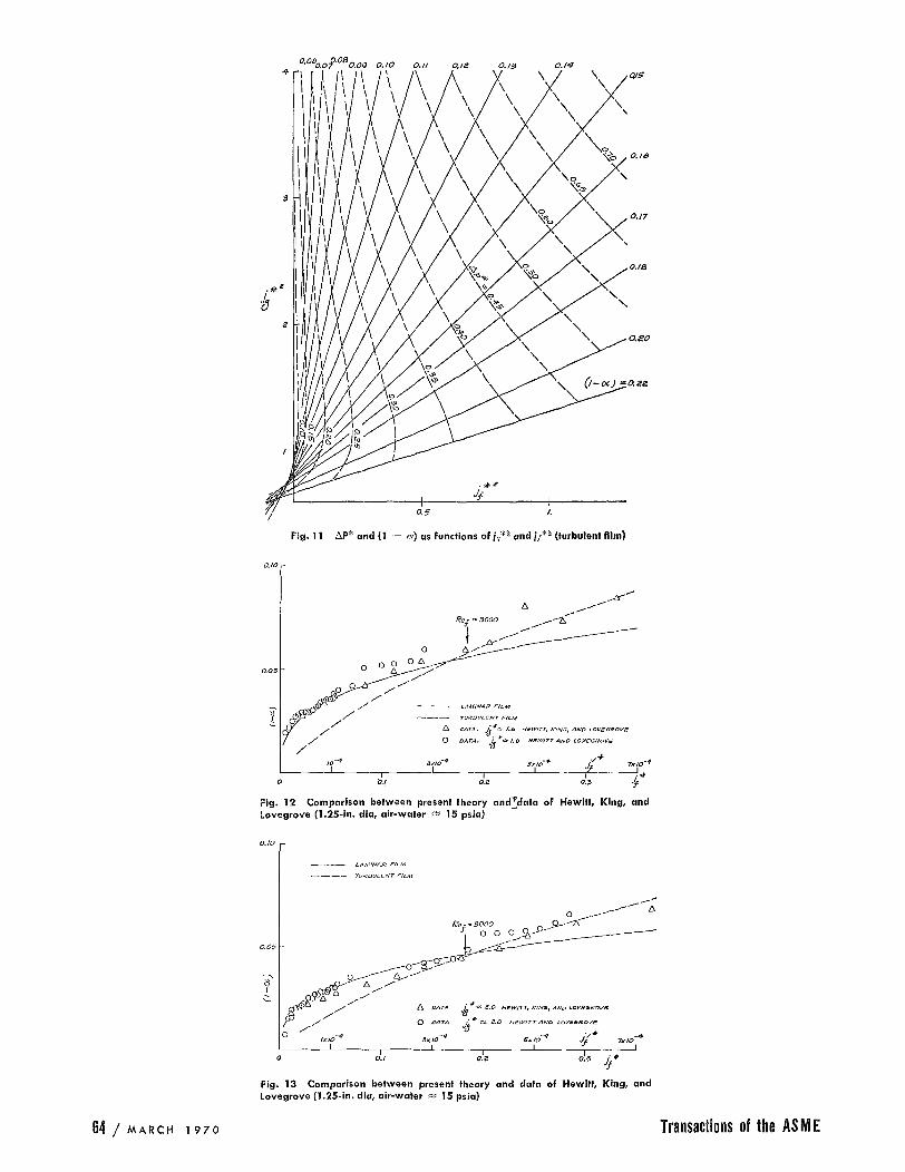
Fig. 14 Comparison between laminar film theory and data of Hewitt, King, and Lovegrove, for high values of / „ * (1.25-in. dia, air-water, 1 5 - 2 0 psia)

o.i

Fig. 15 Pressure-drop data corresponding to conditions of Fig. 14 com­pared with theoretical values

istics and the properties of the device to which it is connected. Fig. 11 also shows that the maximum liquid rate at a given

pressure drop occurs at a value of j 0 * equal to about 1.1 (for AP* < 0.3).

Comparison Between Theory and Data In order to establish the validity of the theory over a range of

conditions, it has been compared with a large variety of data from several sources.

Figs. 12-14 show liquid fraction predictions compared with data of Hewitt, King, and Lovegrove [8], and of Hewitt and Lovegrove [9]. The data are seen to be close to the laminar film prediction up to a value of the liquid Reynolds number of about 3000, and to follow the turbulent film line thereafter. This value of the "transition Reynolds number" is probably not universal, since one would expect some dependence on the gas charac­teristics and perhaps also on the surface tension. Moreover, close to the flow reversal point at jg* « 1, an agitated and plainly turbulent film can exist even when the value of j , (and Re,) is equal to zero.

One cause of deviation from the theory at the higher liquid rates is the significant proportion of the liquid flow which is en­trained in the form of droplets (as reported by Gill and Hewitt [10]). I t would seem that a more sophisticated theory which takes account of this entrainment would lead to greater accuracy. However, the simple theory still provides a reasonable first ap­proximation.

Fig. 15 also shows a reasonable prediction of the pressure drop for the conditions in Fig. 14.

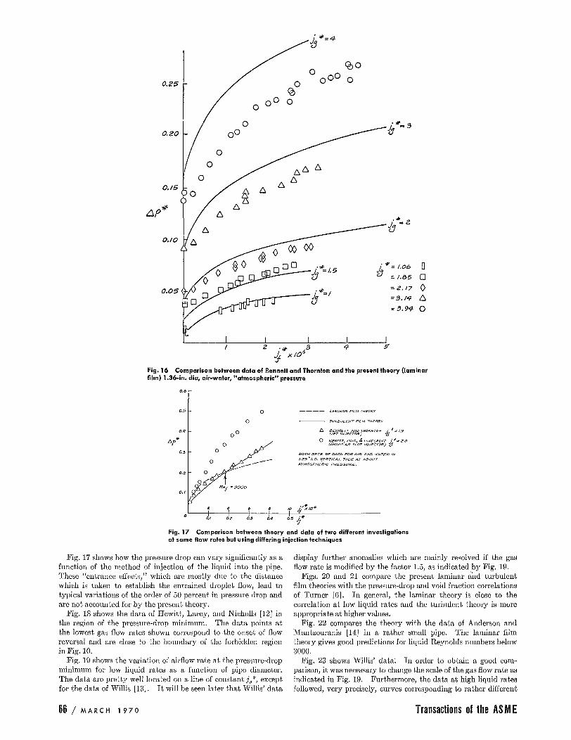
Fig. 16 shows a comparison with the data of Bennett and Thornton [11] for low liquid rates and small amounts of entrain­ment.

Journal of Basic Engineering MARCH 1 9 7 0 / 65

0.25 -

Fig. 16 Comparison between data of Bennett and Thornton and the present theory (laminar film) 1.36-in. dia, air-water, "atmospheric" pressure

TURBULENT FILM THEORY

BOTH SETS OP DATA FOR AIR AND WATER I, 1.25°I.D- VERTICAL- TUBE AT ABOUT ATMOSPHERIC PRESSURE,

Fig. 17 Comparison between theory and data of two different investigations at same flow rates but using differing injection techniques

Fig. 17 shows how the pressure drop can vary significantly as a function of the method of injection of the liquid into the pipe. These "entrance effects," which are mostly due to the distance which is taken to establish the entrained droplet flow, lead to typical variations of the order of 50 percent in pressure drop and are not accounted for by the present theory.

Fig. 18 shows the data of Iiewitt, Lacey, and Nicholls [12] in the region of the pressure-drop minimum. The data points at the lowest gas flow rates shown correspond to the onset of flow reversal and are close to the boundary of the forbidden region in Fig. 10.

Fig. 19 shows the variation of airflow rate at the pressure-drop minimum for low liquid rates as a function of pipe diameter. The data are pretty well located on a line of constant j„*, except for the data of Willis [13]. I t will be seen later that Willis' data

display further anomalies which are mainfy resolved if the gas flow rate is modified by the factor 1.5, as indicated by Fig. 19.

Figs. 20 and 21 compare the present laminar and turbulent film theories with the pressure-drop and void fraction correlations of Turner [6]. In general, the laminar theory is close to the correlation at low liquid rates and the turbulent theory is more appropriate at higher values.

Fig. 22 compares the theory with the data of Anderson and Mantzouranis [14] in a rather small pipe. The laminar film theory gives good predictions for Uquid Reynolds numbers below 3000.

Fig. 23 shows Willis' data: In order to obtain a good com­parison, it was necessary to change the scale of the gas flow rate as indicated in Fig. 19. Furthermore, the data at high liquid rates followed, very precisely, curves corresponding to rather different

66 / M A R C H 1970 Transactions of the AS ME

10

a

5 ><

* a -

<3 6

fe = /3<S>

o.& i to

-

~~

-

1 I 1 \ J \ A

\

/A / £v

/ A /

j A « ^ / X = o.oaaa

/ Jf=.+.bi>XIO-S

/ * / Rex = 310

I I I I 0.0 I I.S 2 i *

J<3

ao r

14 -

5 / 0 U

ZO r

« e / •» 750

J L o.a i

14

Q

V

<t -

_J L 0.0 /

/ * = O.OBS

*=l.75xiO-«

/.3 a i JJ

LAMINAR

TURBULENT

A 20 psia.

O tO psia.

Fig. 18 Data of Hewitt, Lacey, and Nicholls, air and water in 1.25-in. pipe dose to point of minimum pressure gradient

eSr-

— b " 0 HEWITT, LACEY, NICHOLLS,

extrapolated to 15psia. • TURNER A WILLIS O ANOE&SON & MANTZOURANIS

J I L_i_ 0.S I 2 3

TUBE DIAMETER, (INCHES)

Fig. 19 Location of minimum pressure drop at low liquid rales (AP* 0.1) as a function of lube dia; air-water systems at 15 psia Fig. 20 Comparison with Turner's results

Journal of Basic Engineering MARCH 1 9 7 0 / 67

o.&

on

0.5

o.t

0.3

0.1 -

— LAMINAR FILM

- - TURBULENT FILM

- • TURNER 's RESULTS

(/"PIPE, AIR-WATER, IS RSIA)

<\jr*~ U°9

Re,=5500

•-^Z'SZ^--— J Ra, =S70

0.5 1.0 . # i.t>

Fig. 21 Comparison with Turner's results

S.5

o.z C/-oc)

3.0-

AP

SYMBOL

O

D

A

0

IxlO'3

2.2 x/O'3

Ix IO ~*

Z.ZxlO~Z

Rej

Z&O

640

ZbOO

b400

Fig. 22 Comparison between present theory for a laminar film, and data of Anderson and Manfzouranis (0 .427- in. dia, air-water 15 psia)

liquid rates. Perhaps, the method of injection used by Willis which is much more sophisticated than the present analysis, but led to a rather high percentage of entrainment of the liquid flow.

Fig. 24 shows a reasonable compa2"isou with CISE data at high pressure for an argon-water system [15].

Comparison With Levy's Theory

eventually leads to a method for representing the interfacial shear stress. Levy also distinguishes between the conditions AP* j> 1, which determine the curvature of the velocity distribution in the liquid film.

For AP* > 1, Levy plots a function Fl which, in the present Levy [16] has recently presented a theory of annular flow notation with negligible entrainment, is

68 / M A R C H 1970 Transactions of the AS ME

SYMBOL

a o A

r 4.1x10'*

l.3xlO~3

2.2&xl6i

Ref

aoo

bZO

IIOO

THE VAL.S/E OP J*-IS MODIFIED AS EXPLAINED IN THE TEXT

AIR AND WATER AT ATMOSPHERIC PRESSURE IN A 0.502 INCH PIPE

V

0.7

0.6

, 0.5

0.4

0.3

0.2

O.I

# ./"*-, .;* j ' =CKIO-

¥ /^~~jf'2^0-

- *t.y A

A / jf » 1.3 xlO 3

Fig. 23 Pressure-drop data of Willis compared with present theory

A

A OA* •**

o.a

0.15

i-oc)

0.1

0.05

•to a

A

O

Js

4 Fig. 24 Comparison between present theory for a turbulent film and CISE data for argon-water mixtures at 310 psia in a vertical 2.5-cm-ID tube

Journal of Basic Engineering

pi Ti " I 1 A

—J R (44) y.<y. - y,)u>i

R is an empirical function of density ratio shown in Fig. 25 and can be represented quite well by the equation

R = Uf. (45)

Making the following approximations, which are consistent with the level of sophistication of the present theory

Pi » Pa

V„ » V,

Equations (44) and (45) can be combined to give

F 1

Whence, using equation (3),

F1

l_4p0IVJ

4!]'"

(46)

(47)

Levy goes on to plot F1 versus the ratio of the average film thickness to the pipe radius. In view of equation (47), this is just what was done in'Fig. 3 of this paper. We can, therefore, compare the two theories directly by plotting equation (16) on Levy's graphs. The results shown in Figs. 26, 27, and 28 are pleasantly favorable. Large differences occur above a value of 28/D = 0.15, but this is almost certainly in the region of slug-annular flow which usually occurs for (1 — a) > 0.2 [or 28/D £ 0 . 1 ] .

For L\P* < 1 , Levy introduces a correction factor (AP*)1/3 which multiplies the function F1. This factor is never less than V2, and is closer to unity for most of the CISE data considered by Levy. However, it may well be that the addition of the parameter AP* in Fig. 3 could lead to an improvement in accuracy.

I t can be concluded that the present theory is a reasonable approximation to Levy's; it is simpler, but is, perhaps, less ac­curate.

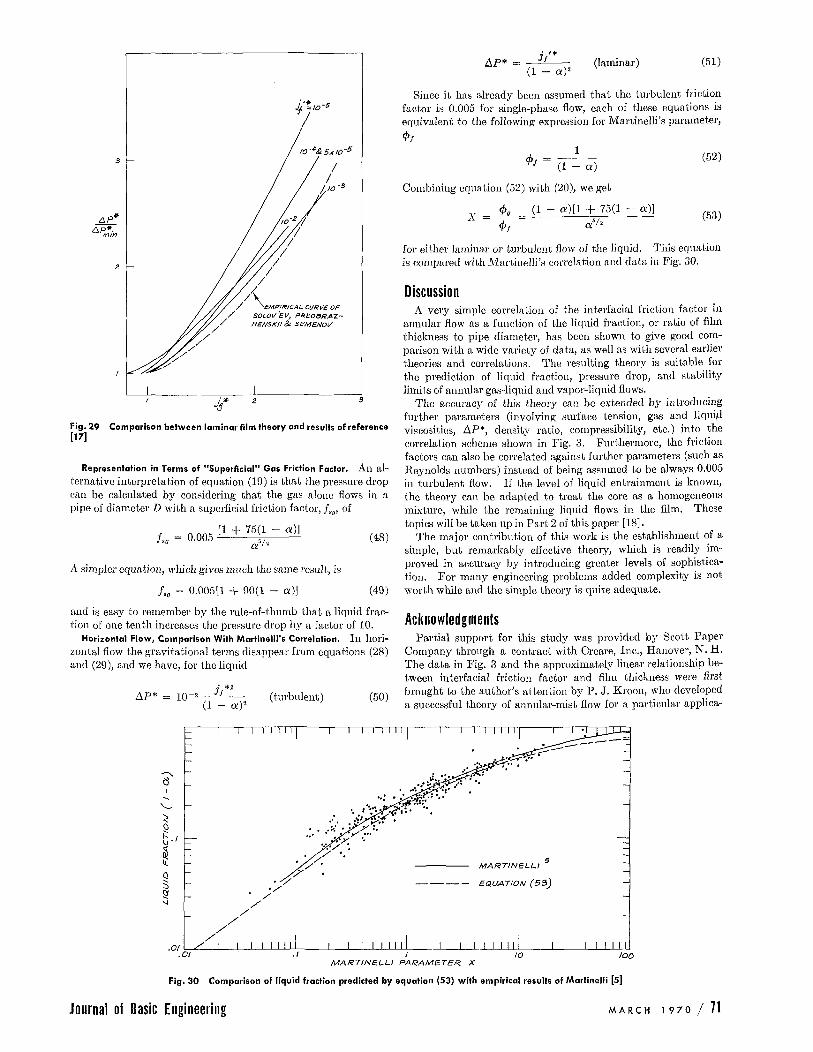
Comparison With Results of Solov'ev, Preobrazhenskii, and Semenov. In reference [17], it was found that a plot of AP*/APmin* versus ja*/jgm- * for a laminar film gave a unique curve for all liquid rates. Fig. 29 shows the present theory plotted in this way as well as the empirical curve from reference [17]. Agreement is surprising considering that j / * is varied over three orders of magnitude. Since j B m m * is approximately constant and is close to unity, the abscissa has been chosen as j g * , although dividing by jg • * gives a slightly better comparison.

too 1000 zooo DENSITY RATIO, /> /p

Fig. 25 Function R of^densify ratio p//pa

MARCH 1 970 / 69

0.3

0.06

0.04

0.03

70 / MARCH 1970

Cl5£ TEST DATA

o WATER IN 2.5 em TUBE

o WATER IN 1.5 em TVBe

4 ALCOHOL IN 1.5 em TV8/:

---- THIS THEORY

LEVY

0.002 0.004 0.007 0.01 0.02 0.04 0.07 0.1 0.2

RATIO OF LIQUID FILM THICKNESS TO PIPe RADIUS, ~o

Fig.26 Comparison between present theory and Levy's correlation of CISE data (vertical flow)

elSE TesT DATA

GAS DENSITY, IO-'G,.ycm" 27.7 22.9 IB.B 16.4 10.0 3.35

WATER IN 2,5cm TVBE 0 4 '7 <> 0 0 WATER IN 1.5 em TV8E •

., • ALCO}-/OL IN 1.5c.m TUBE A .(). -a

L.EVY vZ ~ /'

THIS TH/EORY

Y

Fig. 27 Further comparisons with Levy's work

LEVY

---- PRESENT THEORY

y WICKS-DUKLER ONE INCH TUBE.

0 521 Ibs/h WATER FLOW

'74 <> 1042 0 '7 1563

;"'/ 6. 20B<1-

0 2605

0 311?b

0.01 0.02 0.0"1- 0.1

RATIO OF LIQUID FILM THICKNESS TO PIPE RADIUS 2d 1)

Fig. 28 Comparison with data for horizontal flow

0.3

Transactions of the AS M E

3

2

2 3

Fig.29 Comparison between laminar film theory and results of reference [17]

Representation in Terms of "Superficial" Gas Friction Factor. An al­ternative interpretation of equation (19) is that the pressure drop can be calculated by considering that the gas alone flows in a pipe of diameter D with a superficial friction factor, f80' of

f = 0 OO~ [1 + 75(1 - a)] '0 • D a'/2 (48)

A simpler equation, which gives much the same result, is

j,o = 0.005[1 + 90(1 - a)] (49)

and is easy to remember by the rule-of-thumb that a liquid frac­tion of one tenth increases the pressure drop by a factor of 10.

Horizontal Flow, Comparison With Martinelli's Correlation. In hori­zontal flow the gravitational terms disappear from equations (28) and (29), and we have, for the liquid

• *2 !:J.P* = 10-2 J,

(1 - a)' (turbulent) (50)

. ,* !:J.P* = J,

(1 - a)2 (laminar) (51)

Since it has already been assumed that the turbulent friction factor is 0.005 for single-phase flow, each of these equations is equivalent to the following expression for Martinelli's parameter,

CP, 1

cP, = (1 - a) (52)

Combining eqnation (52) with (20), we get

T CPo (1 - a)[l + 75(1 - a)] X = CPt = a'h

(53)

for either laminar or turbulent flow of the liquid. This equation is compared with lVIartinelli's correlation and data in Fig. 30.

Discussion A very simple correlation of the interfacial friction factor in

annular flow as a function of the liquid fraction, or ratio of film thickness to pipe diameter, has been shown to give good com­parison with a wide variety of data, as well as with several earlier theories and correlations. The resulting theory is suitable for the prediction of liquid fraction, pressure drop, and stability limits of annular gas-liquid and vapor-liquid flows.

The accuracy of this theory can be extended by introducing further parameters (involving surface tension, gas and liquip viscosities, !:J.P*, density ratio, compressibility, etc.) into the correlation scheme shown in Fig. 3. Furthermore, the friction factors can also be correlated against further parameters (such as Reynolds numbers) instead of being assumed to be always 0.005 in turbulent flow. If the level of liquid entrainment is known, t.he theory can be adapted to treat the core as a homogeneous mixture, while the remaining liquid flows in the film. These topics will be taken up in Part 2 of this paper [18].

The major contribution of this work is the establishment of a simple, but remarkably effect.ive theory, which is readily im­proved in accuracy by introducing greater levels of sophistica­tion. For many engineering problems added complexity is not wort.h while and the simple theory is quite adequate.

Acknowledgments Partial support for this study was provided by Scott Paper

Company through a contract with Creal'e, Inc., Hanover, N. H. The data in Fig. 3 and the approximately linear relationship be­tween interfacial friction factor and film thickness were first brought to the author's attention by P. J. Kroon, who developed a successful theory of annular-mist flow for a particular applica-

MARTINELLI '.5

EG/UATION (5:3)

.O/~~~ __ -L-L-L~~~ ____ L--L-L-L~LLUL ____ L-~ __ ~-L~~L ____ -L __ L-L-Li~LU .0/ / /0 100

MARTINELLI PARAMETER X

Fig.30 Comparison of liquid fraction predicted by equation (53) with empirical results of Martinelli [5]

Journal of Basic Engineering MARCH 1970/71

tion. This paper was developed from an unpublished presenta­tion by the author at a symposium organized by the American Institute of Chemical Engineers at Tampa, Fla., May 1968.

References 1 Bergelin, O. P., et al., "Cocurrent Gas-Liquid Flow," Heat

Transfer and Fluid Mechanics Institute, Berkeley, Calif., 1949. 2 Kroon, P. J., Personal communication, 1967. 3 Nikuradse, J., "Stromungsgesetze in rauhen Rohren,"

Forschungsheft, 1933, p. 361. 4 Moody, L. F., "Friction Factors for Pipe Flow," TRANS.

ASME, Vol. 66, 1944, p. 671. 5 Lockhart, R. W., and Martinelli, R. C , "Proposed Correlation

of Data for Isothermal Two-Phase, Two-Component Flow in Pipes," Chemical Engineering Progress, Vol. 45, 1944, p. 39.

6 Turner, J. M„ PhD thesis, Dartmouth College, 1966. 7 Wallis, G. B., "The Transition From Flooding to Upward

Cocurrent Annular Flow in a Vertical Pipe," AEEW-R142, UKAEA, 1962.

8 Hewitt, G. F., King, I., and Lovegrove, P. C , "Holdup and Pressure-Drop Measurements in the Two-Phase Annular Flow of Air-Water Mixtures," AERE-R3764, UKAEA, 1961.

9 Hewitt, G. F., and Lovegrove, P. C , "Comparative Film

Thickness and Holdup Measurements in Vertical Annular Flow," AERE-M1203, UKAEA, 1963.

10 Gill, L. E„ and Hewitt, G. F., "Further Data on the Upward Annular Flow of Air-Water Mixtures," AERE-R3935, UKAEA 1962.

11 Bennett, J. A. R., and Thornton, J. D., "Pressure-Drop Data for the Vertical Flow of Air-Water Mixtures in the Climbing-Film and Liquid-Dispersed Regions," AERE-R3195, UKAEA, 1965.

12 Hewitt, G. F., Lacey, P. M. C„ and Nicholls, B., "Transitions in Film Flow in a Vertical Tube," AERE-R4614, UKAEA, 1965.

13 Willis, J. J., "Upward Annular Two-Phase Air/Water Flow in Vertical Tubes," Chemical Engineering Science, Vol. 20, 1965, pp. 895-902.

14 Anderson, G. H., and Mantzouranis, B. G., "Two-Phase (Gas-Liquid) Flow Phenomena—1," Chemical Engineering Science, Vol. 12, 1960, pp. 109-126.

15 Collier, J. G., and Hewitt, G. F., "Film Thickness Measure­ments," AERE-R4684, UKAEA, 1964.

16 Levy, S., "Prediction of Two-Phase Annular Flow With Liquid Entrainment," International Journal of Heat and Mass Transfer, Vol. 9, 1966, pp. 171-188.

17 Solov'ev, A. V., Preobrazhenskii, E. I., and Semenov, P. A., "Hydraulic Resistance in Two-Phase Flow," International Chemical Engineering, Vol. 7, No. 1, 1967, pp. 59-64.

18 Wallis, G. B., "Annular Two-Phase Flow—Part I I : Ad­ditional Effects," ASME Paper No. 69-FE-46, 1969.

72 / MARCH 1 970 Transactions of the ASME